Improving Cosmological Distance Measurements
Using Twin Type Ia Supernovae

Abstract

We introduce a method for identifying “twin” Type Ia supernovae, and using them to improve distance measurements. This novel approach to Type Ia supernova standardization is made possible by spectrophotometric time series observations from the Nearby Supernova Factory (SNfactory). We begin with a well-measured set of supernovae, find pairs whose spectra match well across the entire optical window, and then test whether this leads to a smaller dispersion in their absolute brightnesses. This analysis is completed in a blinded fashion, ensuring that decisions made in implementing the method do not inadvertently bias the result. We find that pairs of supernovae with more closely matched spectra indeed have reduced brightness dispersion. We are able to standardize this initial set of SNfactory supernovae to $0.083\pm 0.012$ magnitudes, implying a dispersion of $0.072\pm 0.010$ magnitudes in the absence of peculiar velocities. We estimate that with larger numbers of comparison SNe, e.g, using the final SNfactory spectrophotometric dataset as a reference, this method will be capable of standardizing high-redshift supernovae to within 0.06 – 0.07 magnitudes. These results imply that at least 3/4 of the variance in Hubble residuals in current supernova cosmology analyses is due to previously unaccounted-for astrophysical differences among the supernovae.

1 Introduction

Type Ia supernovae (SNe Ia) have a well-established history as standardized candles for cosmological distance measurements. In the late 1990s, studies of high-redshift Type Ia supernovae led to the discovery of the accelerated expansion of the universe – a remarkable and paradigm-shifting discovery (Riess et al. 1998; Perlmutter et al. 1999). Before standardization is applied, among “normal” SNe Ia there exists a dispersion of approximately 40% (Kim et al. 1997). The physical source of this variation is not fully understood, but a number of methods have been developed to reduce this natural dispersion (Vaughan et al. 1995; Riess et al. 1996; Tripp 1998; Wang et al. 2003, 2005; Bailey et al. 2009; Mandel et al. 2011; Barone-Nugent et al. 2012; Kim et al. 2013). The most established approach uses the light curve width and color as standardization parameters. SNe Ia with broader light curves tend to be brighter (Phillips 1993). To some degree, the color correction seems able to account for extrinsic reddening due to dust and intrinsic color differences (presumably arising from differences in the physics of the supernova explosion). With these corrections, the variation in brightness drops to $\sim 15$%, allowing precision cosmology measurements using large samples of SNe Ia.

Since the discovery of the accelerating expansion, many large Type Ia supernova programs have been undertaken, resulting in sufficiently large data sets that statistical errors have become subdominant to systematic errors (Sullivan et al. 2011; Betoule et al. 2014). Much of the effort in reducing systematic errors has focused on the flux calibration of SNe Ia at low-redshift relative to those at high redshift since this error is relatively large and there are clear, though technically challenging, means of addressing it (Juramy et al. 2008; Stubbs et al. 2010; Conley et al. 2011; Tonry et al. 2012; Betoule et al. 2014; Lombardo et al. 2014; Scolnic et al. 2014; Rubin et al. 2015).

If the remaining dispersion of 15% were due to a statistically homogeneous process, then correction of flux calibration issues would clear the way for more large SN surveys using conventional light curve width and color standardization. However, there is ample evidence that the remaining dispersion is not statistically homogeneous. Only relatively recently have significant biases correlated with host galaxy environment been uncovered, and the physical explanation for these observed correlations is still under debate (Kelly et al. 2010; Sullivan et al. 2010; Lampeitl et al. 2010; Childress et al. 2013b; Rigault et al. 2013, 2015). The size of these environmental biases is $\sim 10$%, quite large relative to the standardized brightness dispersion, yet correction for these biases still leaves a significant dispersion (e.g., $\sim 10$% in Rigault et al. (2013, 2015)) that might hide additional astrophysical biases. The diversity of SNe Ia spectral features, which have been ascribed to subpopulations of otherwise normal SNe Ia, also contributes significant systematic errors that are also reflected in the standardize brightness dispersion (Wang et al. 2009; Foley & Kasen 2011; Chotard et al. 2011; Saunders et al. 2015). Dust correction could also introduce systematic errors. There is not only evidence for a variety in the extinction curves of the dust itself (Patat et al. 2015, and references therein), but also for a strong interplay between SN spectral features and the lightcurve “color” appropriate for applying extinction corrections (Chotard et al. 2011; Foley & Kasen 2011).

Suppression of such astrophysical systematics requires separation of intrinsic supernova explosion differences from those of dust. However, disentangling the two has proven a major challenge due to the lack of a clearly identifiable set of observational indicators. Thus, while decreasing the dispersion in standardized brightnesses has a clear statistical payoff, its more important impact is in the implicit suppression of systematic errors.

Techniques to decrease the brightness dispersion continue to be developed. Various spectral metrics have been tried, mostly using spectra near maximum light. For instance, Bailey et al. (2009) were able to achieve a $0.128\pm 0.011$ mag dispersion using a one-parameter spectral correction. This is notable in that this one parameter seems to have captured much of the variation from dust, intrinsic color, and whatever physics is encoded in the lightcurve width (likely total mass; Scalzo et al. (2014)). Another approach has been to attempt to evade dust extinction altogether and to therefore focus on restframe NIR wavelengths. Theoretical modeling suggests that the restframe NIR also may have less intrinsic brightness variation (Kasen 2006). Recent filter-photometry results demonstrate standardization as good as $0.085\pm 0.016$ mag for nearby SNe Ia (Barone-Nugent et al. (2012), Mandel et al. (2011)). These types of studies still do not resolve the fact that some of the observed color arises from dust while some is intrinsic color from the specifics of the explosion.

Using new more detailed measurements of Type Ia supernova time series obtained by the Nearby Supernova Factory (SNfactory; Aldering et al. 2002), we are able to go further in exploring standardization techniques using spectra across all phases. A time series of spectrophotometric observations offers a look at the physics of the explosion through the expanding photosphere. Each phase observation is a snapshot of the elements visible at that stage of the expansion, and their absorption-weighted velocities. If two time series were to match in flux at all wavelengths and times, they would presumably represent the same physical explosion process. Use of such differential techniques is a well-established experimental method for reducing systematics and increasing sensitivity. We call two such time series “twin supernovae”.

A distinct advantage of this twin supernova methodology is the ability to separately account for color arising from dust extinction. The relative amount of dust extinction affecting two spectrophotometric time series can be fit and removed. Any remaining color difference can be ascribed to intrinsic color differences (minus any intrinsic color behavior that happens to exactly mimic the dust color-extinction relation). Two objects that are true twins would have the same intrinsic color and the same spectral features at all times. For pairs of supernovae that are twins, we expect a very small brightness difference, as they represent the same explosion physics. If this is indeed the case, cosmology analyses could treat twin SNe Ia as true standard candles, with no lightcurve width or intrinsic color corrections necessary.

For this analysis, we use spectrophotometric time series with host-galaxy subtractions that are unique to the SNfactory. Much of this dataset is from untargeted searches in the Hubble flow, and thus not only mimics the subtypes of Type Ia supernovae that are found in high-redshift searches, but also is in the redshift regime where host-galaxy peculiar velocity uncertainties are substantially less than the existing dispersion in standardized SNe Ia brightnesses. Ideally, a dataset designed for a twin supernova analysis would consist of frequent observations, to ensure that the analysis captures relevant spectral feature changes. The SNfactory dataset typically has spectrophotometric observations every 2 to 3 nights. Section 2 describes the SNfactory sample used for the twins analysis reported here. Since measurement of dispersion is highly dependent on the tails of the residual distribution, we were careful to finalize the sample selection criteria and analysis methodology before examining the brightness scatter in order to remove the possibility that analysis choices would artificially suppress the dispersion.

Section 2.2 then introduces the techniques we developed to directly compare the supernovae observations to each other. The analysis is discussed in Section 3; we discuss both a near-maximum analysis, and a weighted full time series analysis. In Section 4 the resulting dispersions for each of these analyses is determined. In Section 5, we compare the results to other standardization techniques, and discuss the application of the twins method to new high-redshift SNe Ia, before presenting our conclusions in Section 6.

2 Supernova Data Set

Here we describe the data set used for this analysis. We include details of the observations, a short discussion of the time series interpolation method since it enters into the selection process, and the criteria and outcome of the final sample selection. Steps needed to prepare the data for analysis are also described.

2.1 Observations

The spectrophotometric time series used in this study were obtained by the Nearby Supernova Factory using the SuperNova Integral Field Spectrograph (SNIFS, Lantz et al. 2004). SNIFS consists of a high-throughput wide-band pure-lenslet integral field spectrograph (IFS, “à la TIGER;” Bacon et al. 1995, 2001), a photometric channel to image the field in the vicinity of the IFS for atmospheric transmission monitoring simultaneous with spectroscopy, and an acquisition/guiding channel. The IFS possesses a fully-filled $6.^{\prime\prime}4\times 6.^{\prime\prime}4$ spectroscopic field of view subdivided into a grid of $15\times 15$ spatial elements, a dual-channel spectrograph covering 3200–5200 Å and 5100–10000 Å simultaneously, and an internal calibration unit (continuum and arc lamps). SNIFS is mounted on the south bent Cassegrain port of the University of Hawaii 2.2 m telescope on Mauna Kea, and is operated remotely.

Observations primarily targeted SNe Ia that, at the time, were expected to be at or before maximum light and in the redshift range $0.03<z<0.08$, with a nominal cadence of 2–3 nights. For spectra near maximum, the median signal-to-noise over all SNe and restframe wavelengths 3300–8600 Å is $\sim 42$ per 1000 km s^-1 interval. By comparison, this signal-to-noise is $\sim 18$ for spectra between 20–25 days after maximum. For a typical near-maximum spectrum, this signal-to-noise varies from $\sim 10$ near the wavelength extremes of the two spectrograph channels to $\sim 50$ near their central wavelengths. Multiple spectrophotometric standard stars were regularly observed each night in order to measure the instrument calibration and atmospheric extinction. Parallel imaging was obtained so that it could be employed to remove dimming due to clouds on nights that proved to be non-photometric. Roughly a year or more after the nominal date of maximum, final reference observations were obtained in order to subtract the host galaxy and SN signal.

Spectra of all targets were reduced using the dedicated SNfactory data reduction pipeline, similar to that presented in § 4 of Bacon et al. (2001). A brief discussion of the software pipeline is presented in Aldering et al. (2006) and is updated in Scalzo et al. (2010). Detailed discussions of the flux calibration and host-galaxy subtraction are provided in Buton et al. (2013) and Bongard et al. (2011), respectively. Other spectral and lightcurve results from these data have been presented in Bailey et al. (2009); Chotard et al. (2011); Thomas et al. (2011); Scalzo et al. (2012); Childress et al. (2013a, b); Feindt et al. (2013); Kim et al. (2013); Rigault et al. (2013); Kim et al. (2014); Scalzo et al. (2014); Saunders et al. (2015).

2.2 Interpolation of Supernova Time Series

For the twins analysis it is necessary to compare candidate twin supernovae at the same phases. Realistic observing programs are unable to generate an observation of each SN on every night, so such a comparison requires an estimated spectrum using data at other phases. The quality of such an interpolation affects which spectral time series are appropriate for this study. Here we briefly discuss the method we have implemented.

We have chosen to use Gaussian Process regression (Rasmussen & Williams 2005) to predict SN time series at desired phases. To take advantage of all the available data, in comparing SN_A to SN_B, we first predict SN_A at the phases of SN_B and then vice versa. Each pair is given a ranking (discussed in Section 3.1) by combining the results of both directions.

A Gaussian Process (GP) gives a non-parametric reconstruction of a function from data. It requires the selection of a mean function, which is an initial estimate of the average supernova flux at all phases and wavelengths. We use the spectral template of Hsiao et al. (2007) for our mean function. The end result is not highly dependent on the choice of this mean function, so long as a reasonable function is used, and the gaps in data are not large compared to the typical length scale of the GP mean function. The Gaussian Process uses a kernel to specify the correlation lengths in wavelength and time. For the current analysis, the parameters of the kernel, called hyperparameters, are optimized separately for each SN time series. Once these hyperparameters are found, both the predicted SN flux and an estimate of the flux uncertainty can be generated for any phase of interest. Appendix A details the kernel and hyperparameters used in this analysis.

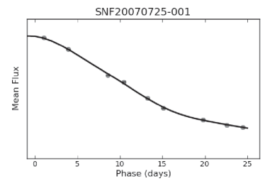
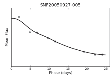
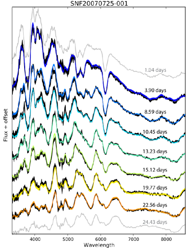
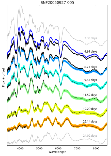
The GP prediction for two supernovae is shown in Figure 1. In this figure, the upper panels show the wavelength-averaged flux for each phase (which is close to the bolometric lightcurve). The lower left panel shows an example of a successful series of predictions: For each SN, we remove each epoch in turn and redo the GP model and predictions. The removed spectrum, in black, is compared to the GP prediction for its date, in color. (We call this a “leave-one-out test.”) The fact that the removed spectra can all be faithfully reproduced indicates that the GP is able to predict this supernova’s spectra at any phase accurately. This was the case for the vast majority ($\sim$83%) of the supernovae. The rarer exceptions, as shown in the right panels, are discussed in the following section.

Figure 1: Wavelength-averaged Gaussian Process predictions for two supernovae. The top images show the wavelength averaged lightcurves. The bottom images show the results of the leave-one out test. The data for each phase are shown in black, and the GP prediction for the leave-one-out test for that phase are shown in color. Left: SNF20070725-001, an example of a supernova that passes the leave-one out test. Right: SNF20050927-005, an example of a supernova which fails the leave-one out test. Several spectra are not reproduced well by the GP prediction of the data at other phases. To be conservative, we drop this supernova while blinded. Note that the first and last data phases (shown in grey) are excluded from the leave-one-out test as we do not expect the GP to be able to extrapolate the endpoints well beyond a few days.

Table 1: Summary of sample selection cuts.

Selection requirement	Included SNe	Included spectra
Initial sample	80	833
Phase $<25$	80	683
First phase $<+2$ days	70	-
Phase gap $<10$ days	67	-
$\geq 5$ spectra	66	591
GP prediction quality	55	468
Full time series	55	468
Near-maximum	49	420

Note. — All of the selection requirements are applied to individual SNe, except for the “Phase $<25$” cut, which applied to individual spectra only, and the “GP prediction quality” cut, which is applied to both individual SNe and spectra. Refer to the text for more details on individual selection requirements.

2.3 Sample Selection

Demonstration of a reduction in dispersion of the standardized peak magnitudes of SNe Ia requires a sufficient number of SNe Ia to measure that dispersion with an uncertainty of $\sim$0.01 mag. This would require at least $N\sim 50$ SNe Ia, if the dispersion is $\sigma\sim$ 0.1  mag, as seen for the best standardization techniques discussed above, and if the accuracy on the dispersion scales as $\sigma/\sqrt{2N}$. Thus we commenced this analysis as soon as the available Nearby Supernova Factory sample reached this approximate size. Once the sample was selected, it was frozen and no further supernovae were added to the sample, as required for a blind analysis. Here we present the details of the sample selection.

As the goal of this study is to measure a dispersion that we anticipate could be much smaller than the canonical $\sim 15$%, it is important to only include SNe Ia having sufficient sensitivity. Broadly speaking, this requires good signal-to-noise, accurate flux calibration and host galaxy subtraction, and temporal sampling sufficient to avoid GP prediction errors. Host galaxy peculiar velocities must be a small fraction of the Hubble expansion velocities so that redshift is a reliable indicator of relative distances. In general, we apply the types of cuts typical of SN cosmology analyses using lightcurve-based standardization since these are what we will be comparing to.

The bulk of the SNfactory dataset is in the range $0.03<z<0.08$. Comparison of two SNe Ia at $z=0.03$ having peculiar velocities of 300 km/s will result in a uncertainty on their relative brightnesses of 14%, so we must exclude the handful of SNe Ia below this redshift. We also set an upper limit of $z=0.1$ since the few SNe above this redshift were observed with much lower S/N than the main program.

Next, we require spectra to have high-quality flux calibration, as described in Buton et al. (2013). This calibration is provided by observations of multiple spectrophotometric standard stars during the night, and on non-photometric nights, a measurement of the loss due to clouds using the SNIFS parallel imaging channel. At least two photometric nights per spectral time series were required in order to ensure adequate reference brightnesses from the parallel imager. We also required final reference datacubes taken under conditions of good seeing, and sufficient for the host galaxy subtraction method presented in Bongard et al. (2011) to converge to a proper solution over the entire portion of sky and host galaxy sampled by each spectral time series. At the time of the start of this analysis, 80 of our SNe Ia satisfied these requirements.

For cosmological analyses where lightcurves are fit using templates or a model, it is typical to require at least 5 lightcurve points, with the first starting no later than 6 nights after $B$-band maximum light (e.g. Suzuki et al. 2012). Such lenient requirements are possible because the templates and models are very stiff and so do not require that all phases be strongly constrained. Because we do not rely on templates or models, and must produce GP predicted spectra for epochs other than those directly observed, our coverage cuts must be more stringent. We perform initial fits with the SALT2.4 lightcurve fitter (Guy et al. 2007; Betoule et al. 2014) to BVR photometry synthesized from the spectrophotometry in order to determine the phases for our observations, and then require that the first spectrum be no later than 2.5 nights after maximum. This requirement results in only very small extrapolation to maximum for SNe Ia whose coverage begins after maximum. We restrict our study to spectra taken before 25 nights after maximum; after this phase SNfactory switched to a much less frequent follow-up cadence. The final cut on coverage is that there can be no gap in coverage greater than 10 nights. Though the nominal SNfactory cadence was 2–3 nights prior to a phase of 25 days, occasionally bad weather, proximity to the Moon, or instrument or telescope operational issues would conspire to create significant gaps. We require a minimum of 5 epochs passing these cuts. After these cuts on coverage, 66 SNe Ia remain.

The above coverage cuts are sufficient for eliminating cases where GP prediction would be strongly suspect, however in a blind analysis we would not be able to further reject SNe traced to bad GP predictions after unblinding, so we deemed it prudent to inspect the predictions more closely while still blinded. First, we examined the GP predictions for visual quality. We required that the wavelength-averaged GP predictions (the upper panels of Figure 1) be smooth as a function of phase. We also performed a leave-one-out test as described in Section 2.2. For supernovae that fail the leave-one-out test, we drop the problematic epoch. If it is not possible to drop the epoch and pass both the leave-one-out test and previous requirements, we drop the supernova all together. Two cases fell below the minimum epoch requirement after this procedure, demonstrating that the temporal distribution is important when there is a small numbers of epochs. Six cases had GP hyperparameters that were not stable under the leave-one-out test, while three others were on the edge of acceptability but rejected as a precaution. Figure 1 shows an example of one supernova that passes these cuts, and an example of another one with similar coverage that fails.

We are left with a final sample of 55 SNe after this last GP prediction robustness check. For the near-maximum analysis discussed in Section 3.1, we require a spectrum within 2.5 nights of maximum in addition to the previous data quality cuts. For that analysis, this leaves a final sample of 49 SNe. The median signal-to-noise of the final sample is $\sim 35$ per 1000 km s^-1 interval for spectra near maximum (calculated as in Section 2.1), and decreases to a median of $\sim 15$ per 1000 km s^-1 interval for spectra at 20–25 days after maximum.

Note that all of these criteria are applied to properties of the observations, not of the supernovae themselves, so this does not bias the selection towards any particular subpopulation of SNe. Additionally, in order to avoid inadvertent bias, the SN selection methodology was decided upon and implemented before the analysis results were unblinded. The number of supernovae and spectra remaining after each stage of cuts is summarized in Table 1.

Figure 2: SALT2.4 fit parameters for both the near-maximum dataset and the full time series dataset. Supernovae shown in blue are in both the near-maximum dataset and the full time series dataset. The supernovae shown in green are those that are dropped from the near-maximum dataset. Left: SALT2.4 $x_{1}$ distribution. Right: SALT2.4 $c$ distribution.

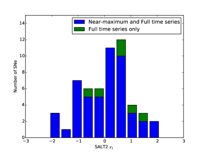
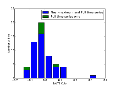
The resulting sample of supernovae has properties that are typical of SNe Ia used in cosmology analyses. The SALT2.4 $x_{1}$ and $c$ distributions for both of these final datasets are shown in Figure 2. The $x_{1}$ distribution is roughly Gaussian with the unit dispersion expected from the $x_{1}$ definition. The color distribution is a positively-skewed Gaussian, as expected — the result of both intrinsic and foreground dust contributions.

2.4 Preparation for Analysis

As a further safeguard against inadvertent bias, the dataset has been divided into training and validation subsamples. The training and validation subsamples were constructed to have similar distributions in lightcurve parameters and host-galaxy properties. We performed all of the initial exploration only on the training sample. When the analysis was finalized, it was applied to the validation sample to act as an independent test and ensure the result was not simply tuned to the training sample. Of the 55 SNe that pass the cuts, 28 are in the training sample, while 27 are in the validation sample. For the near-maximum analysis, 24 are in the training sample, while 25 are in the validation sample. For the full sample, there are 1309 independent pairs of SNe matching our requirements in the full time series sample and 1009 pairs in the near-maximum sample.

Prior to analysis all spectra are first corrected for Galactic extinction based on the Schlegel et al. (1998) dust map, as provided by the NASA Extragalactic Database. Because the SNfactory program specifically avoided SNe with large Galactic extinction, these corrections are small and the uncertainties associated with this correction are negligible. Next, in order to compare spectra, we shift the spectra of all SNe to a common arbitrary redshift in both brightness and wavelength. The redshifts used for this purpose are taken from Childress et al. (2013a). Brightnesses are brought to a common system assuming a $\Lambda$CDM cosmology with $\Omega_{M}=0.28$ and $\Omega_{\Lambda}=0.72$. The specific choice of cosmology is not important since we are working at low redshift where the expansion is linear. Along with this shift to a common redshift, we bin the spectra into 1000 km/s bins from 3300 Å to 8600 Å. This gives a total of 288 bins per spectrum (a resolution of R $\sim 150$).

3 Pairing and Ranking

With our selection of supernovae completed, we develop a method for pairing the supernovae and ranking those pairings, from good twins to non-twins. This method is developed on the training half of the sample before unblinding the results, and then applied to the full sample.

3.1 Near-Maximum Twinness

For the first analysis in this paper, we calculate the twinness using only the spectrum with phase closest to maximum for each SN. For each SN in the near-maximum sample, we compare this spectrum with the GP prediction of every other supernova at that spectrum’s phase. The goal in comparing supernovae to each other is to find pairs that are spectroscopically similar. Any such pairs would be considered “twins.” For our definition of twinness, we choose to use what is effectively a $\chi^{2}$ fit with an error floor. We fit for extrinsic differences between the two supernovae being compared, and call the resulting pseudo-$\chi^{2}$ the “twinness”. Mathematically, we define twinness as follows:

$$\xi(p_{i})=\frac{1}{N_{DOF}}\sum_{\lambda_{j}}\frac{[f_{A}(p_{i},\lambda_{j})-\alpha(\lambda_{j})~{}f_{B}(p_{i},\lambda_{j})]^{2}}{\sigma^{2}_{A}(p_{i},\lambda_{j})+\alpha^{2}(\lambda_{j})~{}\sigma^{2}_{B}(p_{i},\lambda_{j})+(\gamma~{}f_{A}(p_{i},\lambda_{j}))^{2}}$$ (1)

where $f_{A}$ ($\sigma_{A}^{2}$) are the data flux (variance) of SN_A and $f_{B}$ ($\sigma_{B}^{2}$) are the GP-predicted flux (variance) of SN_B. $N_{DOF}$ is the number of degrees of freedom, which is equal to 286 for this analysis (288 wavelength bins with 2 fit parameters). This equation is only defined for a single phase $p_{i}$. $\lambda_{j}$ represent the different wavelength bins, and the sum is over all bins.

A definition of twinness should be made independent of extrinsic dust reddening since it is not a property of the supernova itself. To take dust extinction into account we use the parameter $\alpha$, which is defined as follows:

$$\alpha(\kappa,\Delta E(B-V),\lambda_{j})=\kappa~{}10^{-0.4(a(\lambda_{j})+b(\lambda_{j})/R_{V})R_{V}\Delta E(B-V)}$$ (2)

where the scale factor $\kappa$ captures any remaining overall brightness difference. $\Delta E(B-V)$ captures a Cardelli-like color difference, with $a(\lambda)$ and $b(\lambda)$ defined in Cardelli et al. (1989). $R_{V}$ is fixed to 3.1 for the initial analysis, and 2.8 is used for a later analysis variant.

For each pair of supernovae, $\kappa$ and $\Delta E(B-V)$ are free parameters fit by minimizing the twinness, $\xi(p_{i})$. Twinness fits are performed in both directions, with the GP-prediction of SN_B at the phase of SN_A and then the GP prediction of SN_A at the phase of SN_B. We perform the fits separately because the different phase sampling of the two lightcurves will result in different GP predictions depending on the direction of the comparison. We find that the two values of $\xi(p_{i})$ rarely differ by more than $\sim 10\%$. For each SN pair, the two values of $\xi(p_{i})$ and the two values of $\Delta E(B-V)$ are each averaged. Similarly a single value for $\kappa$ is derived as the geometric mean:

$$\kappa^{\prime}_{AB}=\sqrt{\frac{\kappa_{AB}}{\kappa_{BA}}}$$ (3)

The remaining parameter in Equation 1 is $\gamma$, representing an empirically-determined error floor. Without this term, the definition of $\xi(p_{i})$ will favor pairs of lower signal-to-noise SNe and disfavor high signal-to-noise SNe having even minor spectral differences. $\kappa$ and $\Delta E(B-V)$ are initially fit for each pair with $\gamma=0$. We then introduce a finite $\gamma$ in the final twinness fit so that different pairs can be compared to each other without a strong dependence on their signal-to-noise. We tested the addition of error floors from $\gamma=0.02$ to 0.20 in steps of 0.02 on the training sample. We found that $\gamma=0.12$ produced a ranking of pairs for which the best 50 pairs had a signal-to-noise distribution most similar (evaluated using a Kolmogorov-Smirnov test) to that of the full training set.

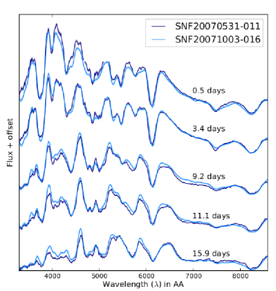
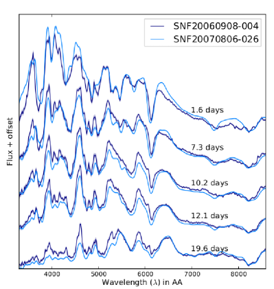
These $\xi$ values give an order to the pairs from “best pairs” to “worst pairs”. Figure 3 shows both a randomly chosen pair out of the best 10% of ordered pairs and a randomly chosen pair out of the worst 50% of ordered pairs. The level of spectral agreement for the good pair, shown in the left panel, is impressive, much better than current theoretical models of supernova explosions are able to achieve (e.g. Röpke et al. 2012). The bad twin example illustrates the lack of spectral agreement in the non-twins regime. Note that, while we show the data at all phases, for the near-maximum analysis the twinness value was calculated using only the spectra closest to maximum.

Since our data are spectrophotometric, $\kappa$ represents the ratio of the absolute brightnesses of the two supernovae. $\kappa$ corresponds to a magnitude difference of:

$$\Delta M=-2.5\,{\rm log}(\kappa).$$ (4)

If $\kappa$ is 1, the supernovae have a magnitude difference of zero. The $\xi$, $\Delta M$ and $\Delta E(B-V)$ values for each pairing of these supernovae are shown in Appendix E. The $\Delta E(B-V)$ values are consistent with differences between SALT2 colors, shown in Figure 2, with a Pearson correlation coefficient of 0.90.

Figure 3: Examples of randomly selected good and bad pairs of supernovae from the training set. Data for the first supernova is shown in dark blue, and the GP prediction for the second one at the phases of the first is shown in light blue. Left: SNF20070531-001 paired with SNF20071003-16. The near-maximum $\xi$ value for this pair is 0.430, which corresponds to the 6th percentile of pairings, low enough to be considered a twin. Right: SNF20060908-004 paired with SNF20070806-026. The near-maximum $\xi$ value for this pair is 1.755, which corresponds to the 77th percentile of pairings — too high to be considered a twin.

3.2 Full Spectral Time Series Twinness

As a variant of this analysis, we also define and calculate values for a twinness metric that operates on the full spectral time series, rather than just the spectrum closest to maximum light. Unfortunately, implementation errors were found in this full time series analysis after unblinding that had to be fixed after unblinding. Although we ran this method with only those specific errors fixed, we nevertheless do not consider our results on the full spectral time series to be blinded. Since the implementation errors are unrelated to any properties of SNe, this portion of the analysis is unlikely to be biased despite not being blind.

In order to make the most of the information from different phases, it is necessary to determine the best relative weights for each phase. The full covariance matrix between all measurements in both phase and wavelength would be ideal for this purpose, but we do not have a way to measure this covariance matrix directly. As an approximation, we estimate $\Delta M$ at each phase using the method described for the near-maximum sample, and we calculate the covariance matrix $C(p_{i},p_{k})$ between these estimates of $\Delta M$. We then take a mean of the pseudo-$\chi^{2}$ values from Equation 1 weighted by this covariance matrix to generate an overall pseudo-$\chi^{2}$ function, as follows:

$$\xi=\frac{1}{N_{DOF}}\frac{\sum_{i,k}C^{-1}(p_{i},p_{k})\xi(p_{k})}{\sum_{i,k}C^{-1}(p_{i},p_{k}),}$$ (5)

which we then minimize. Here $\xi(p_{k})$ is the same as in Equation 1, but without the $N_{DOF}$ term (the $N_{DOF}$ term in Equation 5 is now $N\times 288-2$ where $N$ is the number of phases used, 288 is the number of wavelength bins and 2 is the number of fit parameters). $C(p_{i},p_{k})$ represents the covariance of the dispersion in brightness between phases $i$ and $k$. Application of this equation relies on the ability to calculate the matrix, $C(p_{i},p_{k})$, which is actually a two dimensional function since all of the different supernovae were measured at different phases. Thus, it is necessary to evaluate this function for arbitrary $p_{i}$ and $p_{k}$. The details of estimating this matrix are somewhat technical, and can be found in Appendix B. From the methodology given there, $C(p_{i},p_{k})$ is calculated and used to execute fits to minimize $\xi$ in each direction and thereby obtain a single value of $\kappa$ and $\Delta E(B-V)$ per pairing, as before.

4 Brightness Difference Methodology

Having completed the ordering of supernova pairs, we can assess the extent to which more twin-like pairs (those with low $\xi$) have more similar brightnesses. In this section we describe the measurement of relative brightnesses and the results for the near-maximum and full spectral time series cases. We then describe consistency checks that were performed to validate and better understand the results.

4.1 Magnitude Calculation and Error

Recall that when comparing one supernova to another we fit for a scale factor, $\kappa$, which we convert into a brightness difference $\Delta M$. The uncertainty on this brightness difference is determined from the uncertainty on the fit of $\kappa$, and external uncertainties due to both the host-galaxy peculiar velocities (we assume a 300 km/s uncertainty), and the per-spectrum random gray calibration inferred from standard star measurements (Buton et al. 2013):

$$\sigma_{\Delta M}^{2} =\sigma_{fit}^{2}+\sigma_{ext}^{2}$$ (6)

$$=\sigma_{fit}^{2}+\sigma_{\Delta v_{A}}^{2}+\sigma_{\Delta v_{B}}^{2}+\sigma_{calib}^{2}$$ (7)

where

$$\begin{split}\sigma_{fit}&=(2.5/\ln(10))\,(\sigma_{\kappa}/\kappa)\\ \sigma_{\Delta v}&=(5/\ln(10))\times(300/cz)=0.00217/z\\ \sigma_{calib}&=0.025\end{split}$$ (8)

Note that even with the low redshift cut-off we have imposed, the fit uncertainties ($\sigma_{\kappa}$ and $\sigma_{\Delta E(B-V)}$) are subdominant to the peculiar velocity uncertainties, which comprise roughly 80% of the measurement error budget.

Figure 4: Near-maximum $\xi$ distribution for $R_{V}=3.1$. Due to the long tail of the $\xi$ distribution, we work with the percentile in $\xi$ instead of the raw value itself. Left: Conversion between $\xi$ and $\xi$ percentile. Right: histogram of the near-maximum $\xi$ twinness values.

4.2 Near-maximum results

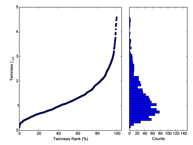
With these considerations in mind, the distribution of near-maximum twinness values $\xi$ for $R_{V}=3.1$ is shown in Figure 4. The histogram on the right shows that there is a broad peak in twinness with a long tail to high values. In order to include this tail, we use the twinness percentile for further analysis instead of the raw twinness score. The pairs of supernovae are then divided into 17 bins of equal twinness percentile, each with 59-60 pairs (17 was arbitrarily chosen because the full spectral time series sample has 1309 pairs, and 17 divides 1309 evenly; it has no deeper meaning and was not fine-tuned in any way). Within each bin the $\Delta M$ values are given uniform weight when calculating the bin dispersions and their uncertainty.

The main result of the twins analysis, using the combined training and validation sample, is shown in Figure 5. On these plots we give the ensemble SN magnitude RMS, which is the appropriate metric for direct comparison with other SN standardization approaches, in each of the 17 pre-defined twinness percentile bins. The measurement errors are small and sufficiently uniform that an unweighted RMS over all values of $\Delta M/\sqrt{2}$ in each bin accurately accounts for the contribution of each SN to the ensemble RMS in that bin. We ran the blind analysis using an $R_{V}$ value of 3.1, however we have reason to believe that an $R_{V}$ of 2.8 (Chotard et al. 2011) may be more appropriate. We report all numbers for both of these values of $R_{V}$, but we consider the $R_{V}=3.1$ analysis to be our pure blinded result. There are few differences between the results with the two $R_{V}$ values, so the following analysis applies to both.

Figure 5: Binned unweighted RMS vs. twinness percentile for the near-maximum analysis. Left: $R_{V}=2.8$, Right: $R_{V}=3.1$. The data is binned by twinness rank, and the data points shown are the unweighted RMS values in each bin. On the left plot, the fit from the main $R_{V}=3.1$ result is shown as a red line for comparison.

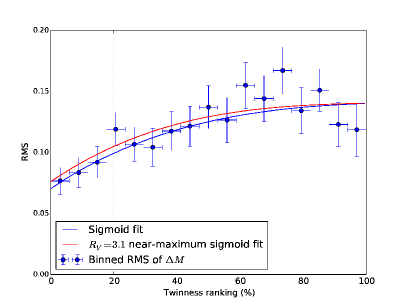
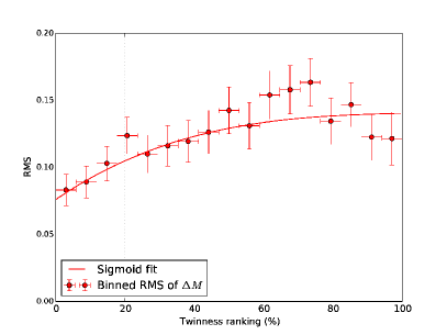
The bin occupancies for each supernova are shown in Appendix D. There is a strong correlation between the dispersions of nearby bins due to the fact that any particular supernova can be included in multiple bins. Errors are estimated on the unweighted RMS in each bin using a Monte Carlo simulation to generate the covariance matrix. We discuss this simulation in Appendix C. We fit a sigmoid model to the unweighted RMS values in each bin with the following form:

$$f(x)=\sqrt{y_{0}^{2}+((y_{100}-{y_{0}})^{2}-y_{0}^{2})\frac{\textrm{erf}(xk)}{\textrm{erf}(100k)}}$$ (9)

The parameters in this expression characterize the observed rise in the RMS vs. $\xi$ data. $y_{0}$ represents the dispersion for the best twins, $y_{100}-y_{0}$ represents the difference in dispersion between the worst and best twins and $k$ affects the shape of the rise. We calculated the significance of observing a decreased dispersion for better twins by comparing the $\chi^{2}$ statistic for both the sigmoid fit and a constant fit using the Bayesian Information Criterion (Schwarz 1978). The Bayesian Information criterion is calculated as BIC $=\chi^{2}+\nu\log(n)$ where $n$ is the number of data points (17) and $\nu$ is the number of free parameters in the fit (3 for the sigmoid, and 1 for the flat line). A $\Delta$BIC larger than 10 corresponds to very strong evidence that one model is favored over another. The results of this comparison are presented in Table 2. For both $R_{V}$ values, the BIC values imply that the improvement in the unweighted RMS for better twins is statistically significant.

Table 2: Change in Bayesian Information Criterion of near-maximum twin result for constant and sigmoid fits

	$R_{V}=2.8$	$R_{V}=3.1$
$\chi^{2}$ for constant	37.90	33.69
$\chi^{2}$ for sigmoid	16.17	13.51
$\Delta$BIC	16.06	14.51

We now focus on the dispersion in the best twinness bin. In principle, with a large reference sample, any new supernova will have many close twins in the reference sample and hence many pairs in this best twinness bin, and these would be the only other supernovae that would be used to determine its relative distance. The quoted values for the unweighted RMS thus correspond to this limiting case. The values and their uncertainties calculated for these dispersions are presented in Table 3.

Table 3: Brightness dispersion for different analyses

Method Variant	Percentile	With peculiar velocity			Peculiar velocity removed
	Cutoff	$R_{V}$=2.8	$R_{V}$=3.1		$R_{V}=2.8$	$R_{V}$=3.1
Pair-wise Analysis
Near-maximum
Training subset	6%	$\mathit{0.073\pm 0.020}$	$\mathit{0.084\pm 0.018}$		$\mathit{0.061\pm 0.016}$	$\mathit{0.074\pm 0.016}$
Validation subset	6%	$\mathit{0.088\pm 0.019}$	$\mathit{0.097\pm 0.020}\tablenotemark{*}$		$\mathit{0.076\pm 0.016}$	$\mathit{0.085\pm 0.018}\tablenotemark{*}$
Combined set	6%	$0.077\pm 0.011$	$0.083\pm 0.012$		$0.064\pm 0.009$	$0.072\pm 0.010$
Weighted full lightcurve	6%	$0.077\pm 0.012$	$0.085\pm 0.011$		$0.062\pm 0.010$	$0.072\pm 0.010$
Realistic, single-SN distance
RMSnw (as measured)	20%	$0.081\pm 0.008$	$0.091\pm 0.009$		$0.069\pm 0.010$	$0.080\pm 0.010$
Large reference sample RMSnw	20%	$0.071\pm 0.007$	$0.079\pm 0.008$		$0.057\pm 0.010$	$0.067\pm 0.010$

Note. — Except where indicated, all results are for the combined training and validation set of SNe.

These results are very promising. The near-maximum study, with $R_{V}=3.1$ (the fully blinded value), yields a dispersion of $0.083\pm 0.011$ mag in the best twinness bin, for the combined training and validation sample. 38 of the 49 SNe Ia in the sample are represented in this bin. This is an impressive improvement over the $\mathrm{0.148\pm 0.015}$ mag dispersion obtained with SALT for exactly the same data. In Section 5.1 we show that this dispersion is among the very best yet achieved among a wide variety of SNe Ia standardization methods. It is interesting to note that the results using $R_{V}=2.8$ (the preferred value from Chotard et al. (2011)), appear to be slightly better: we obtain $0.077\pm 0.011$ mag for the dispersion in the best twinness bin.

Since we are working at low redshift, peculiar velocities account for a significant portion of the spread in magnitude. Therefore it is instructive to estimate the dispersion that would result without the peculiar velocity component, as might be seen with a high-redshift SN sample. Using a dispersion estimate of $\Delta v=300$ km/s for the peculiar velocities and assuming that they are all independent, we calculate their contribution to the unweighted RMS and removed it. We find that without peculiar velocities the near-maximum twins dispersion drops to $0.072\pm 0.010$ mag. The results with peculiar velocity dispersion removed are shown in the right two columns of Table 3.

If we break the supernova sample into its training and validation subsamples, we find consistent results. For these two subsamples the RMS values in the first bin are tablulated in the first and second rows of Table 3. For the training sample the RMS values in the first bin range from $0.061$ to $0.084$ mag for the different analyses. For the validation sample this range is $0.076$ to $0.097$ mag. The validation RMS values are between $0.011$ to $0.015$ mag higher than the training RMS values, but this is well within the $\sim 0.025$ mag uncertainty between these two independent subsets of SNe, and thus not statistically significant. Note that the RMS values of both the training and validation subsets are slightly higher than for the combined sample since SNe are less likely to find a good twin in a smaller sample (in Section 5.3 we discuss the further improvement in RMS expected for yet larger samples). The following results use the combined training and validation sets.

4.3 Full Spectral Time Series Analysis

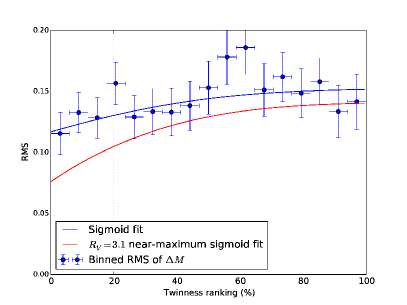
The full spectral time series twinness definition from Section 3.2 was used to examine dispersion as a function of twinness, just as for the near-maximum analysis described above. Plots of RMS as a function of $\xi$ for the full spectral time series are shown in Figure 6.

Figure 6: Binned unweighted RMS vs. twinness percentile for the weighted full spectral time series analysis. Left: $R_{V}=2.8$, Right: $R_{V}=3.1$. The fit from the main $R_{V}=3.1$ near-maximum result is shown as a red line for comparison.

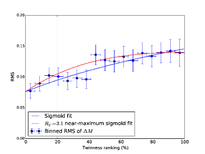
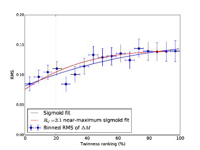
The full spectral time series twinness values do produce better results overall than the near-maximum only values. However, most of the gain comes from the 20–40th percentile range. The unweighted RMS values for the first bins are shown in Table 3 (43 out of 55 SNe are represented in the best bin for the $R_{V}=3.1$ analysis). These RMS values agree almost exactly with the near-maximum result indicating that we do not gain much, if anything, by including later phases for good twins. Again, the Chotard et al. (2011) value of $R_{V}=2.8$ gives slightly better results.

4.4 Consistency

In this section we present checks on the internal consistency of our measurements, and their relation to SALT. First, we examined what a traditional standardization would give for the same dataset: we calculated corrected magnitudes for each SN using the Tripp (1998) lightcurve width and color relation with $x_{1}$ and $c$ from SALT2.4 fits. The dispersion of these corrected magnitudes is $\mathrm{0.148\pm 0.015}$. We investigated whether the twinness can be used to improve the SALT-based standardized magnitudes, and we show the RMS values using these magnitudes as a function of twinness in Figure 7. This figure shows a weak dependence on twinness, but the results are nowhere near as good as the twins method in the best twins bins. This implies that the twins analysis is capturing more information than a conventional standardization based on color and stretch parameters.

Interestingly, the dispersion taken over all bins, i.e. ignoring twin rank, is $0.128\pm 0.012$ mag. This outperforms the dispersion resulting from the SALT-based standardization. We believe that this is due to the fact that SALT lightcurve fits do not use the full wavelength range and resolution of our spectra. To explore this, we created a basic SALT fitter that uses the SALT templates over the full spectrum with the full wavelength range and same wavelength resolution used in the twins analysis. Standardization using peak magnitude, $x_{1}$ and $c$ from this fitter gives an overall dispersion of $0.133\pm 0.013$ mag which is consistent with the overall twins RMS. There is no significant dependence of the RMS values calculated using this method on twinness, so the pairwise method still has a much better dispersion if only the best twins are considered. Thus, there appears to be extra information available in a direct comparison of two spectra that is not captured in the two parameter model in a SALT-based standardization.

We also checked whether the twins result improves when removing the remaining correlation of RMS with SALT $x_{1}$ and $c$. This does not improve the result for good twins, which is expected since good twins should have very similar lightcurve widths, while the color has been taken out as part of the twinning calculation. It does improve the results somewhat for the worst twins, where we do not expect the twins method to work well; the twins method is designed to simply reject those pairings rather than attempt to match them.

Figure 7: Binned SALT unweighted RMS vs. near-maximum twinness rank (percentile). The near-maximum twins RMS fit with $R_{V}=3.1$ is shown as a red line for comparison. Magnitude differences calculated with SALT show only a weak dependence on twinness.

In all the previous analyses, we only calculate the difference in brightness and colors between two supernovae, never the actual values for individual supernovae. As a consistency check, we fit for a global set of self-consistent magnitude and color differences for each supernova. This gives a consistent set of values that are commutative. When comparing the $\Delta M$ and $\Delta E(B-V)$ values from the global fits to those calculated with the twins method, the difference $\Delta M_{\text{fit}}-\Delta M_{\text{twins}}$ has an RMS of 0.030 mag and the difference $\Delta E(B-V)_{\text{fit}}-\Delta E(B-V)_{\text{twins}}$ has an RMS of 0.0095 mag. These values are small compared to the sample dispersions and indicate good agreement.

5 Discussion

We now turn to several considerations concerning the application of the twins method for cosmology. We begin by comparing our result with the dispersions and efficiencies attained by other SN Ia standardization techniques. Next, we explore how realistic distance determinations can be made using the twins method, and whether we can obtain distances with uncertainties as small as the dispersions discussed in Section 4. Finally, we consider how the uncertainty on these distance determinations is expected to scale with the size of the reference sample.

5.1 Comparison to Other Standardization Techniques

For the near-maximum twins analysis we found a dispersion of $0.083\pm 0.012$ mag using $N=38$ of the 49 SNe Ia in the sample. This is a substantial improvement over the SALT dispersion of $\mathrm{0.148\pm 0.015}$ mag found using the same data. The literature contains a number of results showing small dispersion, to which our result can be compared. For this purpose, we quote the best dispersion presented in each paper. To be consistent with our values, no measurement uncertainties were subtracted for these studies. When uncertainty on the dispersion was not provided, we calculated it assuming a Gaussian distribution for the magnitude residuals.

The very best alternative standardization techniques include the results of Barone-Nugent et al. (2012), who achieved $0.085\pm 0.016$ mag using NIR lightcurves for all $N=12$ SNe Ia in their sample; Wang et al. (2003), who achieved a dispersion of $0.080\pm 0.013$ using the CMAGIC technique and cuts that included $N=20$ of their 40 SNe Ia; and Kelly et al. (2015), who achieved a dispersion of $0.065\pm 0.016$ by using SALT2.4 lightcurve parameter standardization and then selecting the $N=10$ of their 50 SNe Ia having the highest local star formation rate. Our result is equally good, but includes many more SNe Ia than these studies.

Several more alternative standardization techniques report dispersion values that are higher than, but statistically consistent with, ours: Foley & Kasen (2011) found a dispersion of $0.109\pm 0.010$ mag using the $N=65$ of their 121 SNe Ia having a normal velocity for the Si II $\lambda 6355$ Å absorption line; Rigault et al. (2013) obtained a dispersion of $0.105\pm 0.012$ mag using SALT2.4 and $N=41$ of their 82 SNe Ia by taking the half of their sample having the highest local star formation rate; Mandel et al. (2011) obtained a dispersion of $0.101\pm 0.019$ mag using a hierarchical Bayesian model applied to 37 SNe Ia having both optical and NIR imaging lightcurves and $0.113\pm 0.016$ mag using 57 SNe Ia having both optical and NIR imaging lightcurves.

Thus, the twins method produces a dispersion that is as good, if not better than, the best known standardization methods to date, especially considering that these comparison studies were performed unblinded. In addition, the efficiency in using SNe Ia is among the highest (78%), and the size of the sample from which the dispersion is measured is among the largest.

5.2 Realistic Application to a New Single Supernova

If a set of spectrophotometrically observed high-redshift supernovae became available, the twins methodology could be applied (the currently considered design for the WFIRST space telescope mission (Spergel et al. 2015) could provide such a sample). A large sample of low-redshift SNe Ia adjusted to a common redshift would serve as a set of templates against which the high-redshift sample is fit. The brightness for each high-redshift SN relative to all the low-redshift supernovae it matches well could be calculated using the method described in Equation 1. Taking a number-weighted average of these $\Delta M$ values would produce an average brightness difference, which we denote as $\phi_{i}$, for each high-redshift supernova indexed by $i$. Then $\phi_{i}$ is a measure of the relative distance modulus, given by:

$$\phi_{i}(\xi_{\rm{cutoff}})=\frac{\sum_{j,~{}\xi_{ij}<\xi_{\rm{cutoff}}}\Delta M_{ij}}{\sum_{j,~{}\xi_{ij}<\xi_{\rm{cutoff}}}1}$$ (10)

To mimic this situation within our low-redshift sample, we treat each supernova in turn as though it were the high-redshift supernova. Note that because the redshifts have been adjusted to a common redshift in this sample, $\phi_{i}$ would be zero for a perfect standard candle with no measurement errors. Hence the spread of those $\phi_{i}$ values over this sample measures the dispersion in this standardization method.

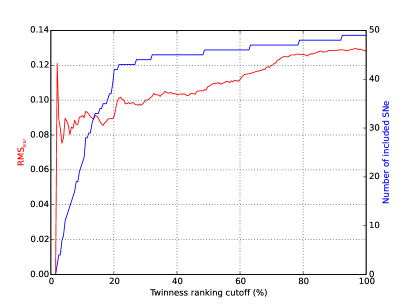
To apply this to our sample, we find all the supernovae that have at least four pairs below some cutoff, $\xi_{\rm{cutoff}}$, (that is, at least four good twins) and we calculate the number-weighted root-mean-square (RMS_nw) of the distance moduli $\phi_{i}(\xi_{\rm{cutoff}})$ as our measure of spread. At least four pairs are required so that their $\phi_{i}$ values are reasonably well defined; we tested that the results are similar with a requirement of at least three or at least five pairs. We calculate this RMS_nw as a function of $\xi_{\rm{cutoff}}$: we let in worse and worse-twinning pairs to the calculation of the $\phi_{i}$ values. We expect the RMS_nw($\xi$) to increase with $\xi_{\rm{cutoff}}$, as more and more non-twin pairs are included. To summarize, the RMS_nw formula is:

$$\text{RMS${}_{nw}$}(\xi_{\rm{cutoff}})=\sqrt{\frac{\sum_{i}\left(\phi_{i}(\xi_{\rm{cutoff}})^{2}(\sum_{j,~{}\xi_{ij}<\xi_{\rm{cutoff}}}1)\right)}{\sum_{i,~{}j,~{}\xi_{ij}<\xi_{\rm{cutoff}}}1}}$$ (11)

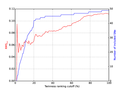
The left panel of Figure 8 shows the RMS_nw as a function of $\xi$ rank for the near-maximum, $R_{V}=3.1$ analysis. Setting a cutoff at a $\xi$ rank of 20% as an example, we arrive at a dispersion in the $\phi_{i}$ values of 0.091 mag, with 85% of the supernovae included. This result is tabulated in the fifth row of Table 3. The other 15% of SNe Ia that did not have good twins could still be included albeit with a larger uncertainty. With a larger low-redshift reference sample, we would expect that more of these supernovae would find enough pairs to be included in our sample, and we lose very few of these. Nevertheless, for cosmology purposes, losing part of the sample is acceptable since the low dispersion means that the SNe that are included have more value. Additionally, there is less chance of systematic error due to an evolutionary drift in SN population properties.

Figure 8: Number-weighted root mean square (RMS_nw) as a function of twinness rank ($\xi$) cutoff for a realistic, single-supernova distance determination. The red line shows the RMS_nw, and the blue line shows the number of included SNe. Left: Near-maximum, $R_{V}=3.1$ analysis. Right: Same analysis with peculiar velocity and finite reference sample corrections applied.

5.3 Improvements with Future Samples

At high redshifts, the effects of peculiar velocity would be negligible, however, this current application analysis is affected by peculiar velocity since we are comparing low redshift supernovae to each other. As described in the previous section, and shown in the right two columns of Table 3, the result with negligible peculiar velocity uncertainties can be estimated by assuming that each SN is affected by equal and independent amounts, here taken as $\Delta v=300$ km/s, and removing this contribution from the RMS_nw. Note that this analysis is only for the purpose of estimating the likely dispersion for high-redshift SNe; we assume there will always be a low-redshift sample for which uncertainties due to peculiar velocities are relevant, and therefore we do not remove this part of the dispersion. However, for a large low-redshift reference sample, the uncertainty due to random peculiar velocities would be small, approaching the amplitude of any coherent uncorrected bulk flow spanning the sample volume (Hui & Greene 2006).

Currently there is an additional penalty due to the fact that a limited number of supernovae were available for comparison at the time the sample for this study was frozen. Propagating the error on the $\Delta M$ values, and assuming that even for twins there remains a finite intrinsic dispersion, $\sigma$, that is the same for every supernova, the uncertainty on $\phi_{i}$ is given by:

$$\sigma_{\phi_{i}}=\sigma\sqrt{1+\frac{1}{\sqrt{N_{used}}}}$$ (12)

where $N_{used}$ is the number of pairs used in the estimate of $\phi_{i}$, and the RMS_nw in Equation 11 is an estimator of this $\sigma_{\phi_{i}}$. Hence we can estimate the result that would be obtained with a large sample, i.e., where the number of pairs, $N_{used}$, is not a limitation, by dividing by the term on the right in Equation 12. These results are shown in the last line of Table 3.

For such a large sample, and also removing the peculiar velocity dispersion, we obtain the result shown in the right panel of Figure 8. Here, with a cut on twinness rank at 20% and using $R_{V}=3.1$, we would expect $\sigma_{\phi_{i}}\sim 0.067$ mag with 85% of the sample included. For the $R_{V}=2.8$ analysis, we would expect $\sigma_{\phi_{i}}\sim 0.057$ mag. The simple approach of Section 5.2 for realistically implementing the twin method thus, in the limit of a large sample size, gives results consistent with the RMS results shown for the pair-wise analysis of Section 4.

Future use of the $\sim$200–300 SNe Ia anticipated in the final SNfactory dataset as a reference is expected to gain much of this large-sample dispersion improvement. The value of $N_{used}$ in Equation 12 will scale up in proportion to the overall sample size. Therefore, we forecast that this sample of $\sim$200–300 SNe Ia already will be sufficient to reduce the dispersion to $\sigma_{\phi_{i}}\sim 0.073$ mag. For $R_{V}=2.8$, $\sigma_{\phi_{i}}\sim 0.062$ mag would be expected.

Enlarging the sample should also improve both the quality of the best twins and the number of supernovae that are able to find twins. Empirically, we found a 20% decrease in the dispersion when the training sample was combined with the validation sample. The finite reference sample correction only predicts a 6% decrease, so the majority of this improvement is likely due to the supernovae in the full sample having better twins available. In the most optimistic scenario, where there is no dispersion in brightness between supernovae that are truly twins, the relative brightness uncertainty will be entirely limited by how well matched the best twins available in the reference sample are for a new supernova. We note that we observe this extra decrease in dispersion, but this improvement depends heavily on the properties of any subpopulations of SNe Ia, so we cannot predict how rapidly the dispersion will improve as the sample size grows. Future studies with larger reference samples will be able to measure the true dispersion of the best twins, and determine whether it varies for subpopulations of SNe Ia.

The twins method has obvious cosmological applications nearby, such as measuring distances to nearby galaxies and mapping the peculiar velocity field. In future work, we will explore the performance characteristics of the twins method as a function of resolution and signal-to-noise. In the current analysis, the SNIFS data were binned to a resolution of R $\sim$ 150. Our lowest signal-to-noise spectra have a signal-to-noise of $\sim 12$ at this resolution and show no signs of degradation in their brightness dispersion for best twins. These data characteristics are modest, suggesting that the twins technique is likely to be within reach of experiments such as JWST and WFIRST, even at high redshifts.

5.4 Phase Determination from Lightcurve

An important implementation consideration is that the twins analysis requires knowledge of the phase of a spectrum when comparing it to the reference sample. Currently, this is done using a SALT2.4 fit to a full lightcurve. An experiment that applied the near-maximum version of the twins method would need to obtain one good spectrum near maximum along with crude photometry at other points on the lightcurve sufficient to provide the date of maximum. It may be possible to estimate the date of maximum directly from the twins method, along the lines of existing SN typing codes, but this has not yet been attempted and is left for future work.

The uncertainty of the phase determination will propagate into the final uncertainty on the relative distance. For our sample, the median uncertainty on the day of maximum is 0.28 days, which means that we have an uncertainty of 0.4 days on our phases when comparing two SNe. We redid our analysis with Gaussian Process predictions offset from the measured maximum phase to get an estimate of the contribution to the brightness dispersion from phase errors. For a 0.4 day offset, we get an additional dispersion of 0.03 mag, while for a 1 day offset we get an additional dispersion of 0.05 mag. Note that these values are upper limits on the contributions to the dispersion since we have introduced new phase errors in addition to the ones already present in the data. Regardless, this uncertainty is still significantly smaller than even the smallest dispersion listed in Table 3, so the phase error cannot be the main contributor. Future experiments will apparently need to constrain the day of maximum of SNe to an accuracy comparable to that of the current analysis if they are to obtain comparably tight magnitude dispersions.

6 Conclusions

We have shown that Type Ia supernovae that are spectroscopic twins have a lower luminosity dispersion than spectroscopically dissimilar Type Ia supernovae. Rather than using the lightcurves to standardize the supernova samples, future surveys could standardize supernovae employing a single spectrum measured near maximum and applying the twins method. With the subset of SNfactory data used in this paper, the twins method can standardize supernovae to $\sim$0.08 mag at low redshifts. After removing uncertainties due to host-galaxy peculiar velocities the resulting dispersion would be $\sim$0.07 mag. This is the value expected at high redshifts, where the fractional contribution due to peculiar velocities is negligible. It is estimated that the twins method may be able standardize high-redshift supernovae with a dispersion of 0.06–0.07 mag once a larger sample becomes available as a reference. The twins dispersions are as good as the best known standardization methods to date. While implicit in the concept of twin SNe Ia, future work, requiring a larger sample, will be needed to study the extent to which the non-parametric twins method subsumes other parametric standardization methods.

An important question in supernova cosmology studies is what portion of the observed distance dispersion is due to astrophysical differences among the supernovae that are not accounted for by current analysis techniques. Our results imply that at least 3/4 of the variance in Hubble residuals from a SALT-like lightcurve-based standardization is due to such differences among the supernovae. That is, the SN astrophysical variation dominates over other common concerns, such as variation in dust extinction laws and uncorrelated calibration errors.

Our analysis shows that spectrophotometric data of supernovae is extremely valuable, and we find a low dispersion even if only a single spectrum is taken near maximum. This standardization method also has the advantage that it does not require rest-frame infra-red data, so it can be used for supernovae at much higher redshifts than is possible with standardization that requires such data, given current and planned near-IR observing capabilities.

The fact that the magnitude dispersion dramatically improves for better twins — whether or not the magnitudes are standardized using conventional methods — implies that there are subpopulations of Type Ia SNe with different mean absolute magnitudes that can be recognized by their spectra. The relative frequency of these different SNe Ia affects the mean brightness of an ensemble measured at a given redshift. Thus, if the demographics of the SNe Ia changes with redshift (e.g. Rigault et al. 2013; Childress et al. 2014; Rigault et al. 2015), current measurements of the cosmological parameters could be biased. The twins analysis is, in principle, capable of handling any drift in the demographics of the SN Ia population with redshift without any modifications. If all major subpopulations are well represented in the reference sample, the twins method will be comparing new SNe to reference SNe within their subpopulations. The method is therefore limited only by the inherent dispersion of the subpopulations. Unusual SNe, or previously unobserved subpopulations of SNe, can be identified and rejected automatically since they will not twin well with any SNe in the reference set.

Further work is needed to determine the minimal spectral information required to achieve these twin results. In addition, while weighting by the covariance between different phases has been explored here, it is possible that weighting by the covariance between both phases and wavelengths might produce an even smaller dispersion. The final SNfactory dataset will be much larger, allowing such a broader range of studies. The twins method could also be applied to analyses of supernova subtypes beyond those pioneered by Branch et al. (2006). The twinness rank, $\xi$, provides a natural way to quantitatively identify subtypes of Type Ia supernovae based on groups of closely matched SNe.

Appendix A Gaussian Process Regression

We train a Gaussian Process to perform interpolation on our data with the following parameters. For the mean function, we choose the spectral template of Hsiao et al. (2007) and allow one hyperparameter, $\theta_{a}$, to handle the overall flux normalization. Note that the mean function is what the GP prediction will default to in the absence of coverage by training data. For our kernel, we use a squared exponential of the form:

$$k\begin{pmatrix}\begin{bmatrix}\mathrm{ln}~{}\lambda_{i}\\ t_{i}\end{bmatrix},\begin{bmatrix}\mathrm{ln}~{}\lambda_{j}\\ t_{j}\end{bmatrix}\end{pmatrix}=\theta_{s}^{2}\mathrm{exp}\begin{pmatrix}-\frac{1}{2}\begin{bmatrix}\mathrm{ln}~{}\lambda_{i}-\mathrm{ln}~{}\lambda_{j}\\ t_{i}-t_{j}\end{bmatrix}^{T}\begin{bmatrix}1/\theta_{\lambda}^{2}&0\\ 0&1/\theta_{t}^{2}\end{bmatrix}\begin{bmatrix}\mathrm{ln}~{}\lambda_{i}-\mathrm{ln}~{}\lambda_{j}\\ t_{i}-t_{j}\end{bmatrix}\end{pmatrix}+\theta^{2}_{n}\delta_{t_{i},t_{j}}$$ (A1)

We use the difference in $\mathrm{ln}~{}\lambda$ as opposed to $\lambda$ since velocity space is more physically relevant to supernova explosions. $\theta_{s}$ is the amplitude hyperparameter and gives the scale of the GP prediction error when sufficiently far away from training data. $\theta_{\lambda}$ and $\theta_{t}$ are, respectively, the length scales in log wavelength and time. $\theta_{n}$ is the time nugget, which differs from noise in that it is non-zero only when two data points are at the same phase, and accounts for wavelength-independent calibration errors and noise.

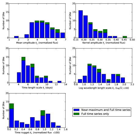
We use maximum likelihood estimation for each individual time series to calculate the hyperparameters for the mean and the kernel simultaneously. We use Minuit2 as our optimizer (James & Roos 1975). We are then able to use these optimized hyperparameters to make predictions at any desired wavelengths and phases. Figure 9 show histograms of the hyperparameter values for each of the five hyperparameters used in this analysis. The range of values for each of these hyperparameters is reasonable.

The supernovae have been shifted to a common redshift, so we expect $\theta_{a}$ to have a similar dispersion as uncorrected supernovae in flux space, and that is indeed what we see. For the time length scale, $\theta_{t}$, we have values ranging from $\sim$4 to $\sim$12 nights. Although SNe Ia vary on few day timescales (as is evidenced by examination of their spectra), this hyperparameter value is affected by the data sampling as well as the overall smoothness of the data since a shorter time length scale will allow for more variation in the GP predictions. The range of $\theta_{\lambda}$ corresponds to velocities between $\sim$2250 km s^-1 and $\sim$7750 km s^-1. Or, in terms of wavelength, $\sim$25Å-85Å at the blue end and $\sim$65Å-215Å at the red end. This is a reasonable range given that SN feature widths are typically several thousand km s^-1.

Figure 9: Histograms of the various hyperparameters for the supernovae in both the near-maximum and full time series samples. Top left to bottom left are: mean amplitude ($\theta_{a}$), kernel amplitude ($\theta_{s}$), time length scale ($\theta_{t}$), log wavelength length scale ($\theta_{\lambda}$), and time nugget ($\theta_{n}$)

Appendix B Phase Weighting Covariance Matrix

For the full spectral time series analysis in Section 3.2, the correlation in brightness dispersion between any two phases, $C(p_{i},p_{k})$ needs to be determined. We estimate this function from the data. This is done by performing a calculation as in the near-maximum study centered around all of $-5,0,5,10,15,20$ and $25$ days after maximum. The correlation matrix of these data is calculated using the subset of pairs that is in each of the phase bins. It is worth noting that different pairs of supernovae can be missing in different samples depending on the cadence of their observations. Hence not all of the same pairs are used for each entry in this correlation matrix, making it very poorly conditioned.

In order to be useful the correlation function must work given any two phases $p_{i}$ and $p_{k}$, not just two chosen from the samples above. To regularize the computation, we assume that the correlation between two phases is given by:

$$D(p_{i},p_{k})=\exp(-\alpha|p_{i}-p_{k}|)$$ (B1)

and we then solve for $\alpha$ by fitting to the results from the above sample. We obtain $\alpha=0.053\text{~{}day}^{-1}$ for $R_{V}=3.1$ and $\alpha=0.060\text{~{}day}^{-1}$ for $R_{V}=2.8$. Note that this indicates a very high correlation between nearby phases, so only limited information is gained from adding additional nearby phases. Interestingly, $\alpha^{-1}\sim 16$ days. This is comparable to the 15 day difference in brightness $\Delta M_{15}$ that is commonly used to standardize supernovae (Phillips 1993).

We are interested in optimizing the weighting for good twins rather than for the sample as a whole. Hence, when calculating the variance, we apply the near-maximum twinning algorithm for each sample independently, and we take the variance of the best 10% of twins in each sample. Ideally we would only use the best 10% as well when calculating the full covariance matrix, but our sample size is currently too small to make this statistically feasible since overlapping pairs are required when calculating the correlation between two bins. A spline is then fit through the calculated variances in order to interpolate to any phase. Combining the correlation and variances, we can calculate the covariance matrix $C(p_{i},p_{k})$ for any combination of phases.

Appendix C Monte Carlo simulation

We used a Monte Carlo simulation to calculate the covariance of the RMS bins. The Monte Carlo simulation involves the following steps:

1. Generate a probability density function (PDF) of the distribution of magnitudes.

2. Generate a PDF of the distribution of twinness for each value of $\Delta M$.

3. Randomly choose a set of magnitudes from the magnitude distribution to generate a mock sample.

4. Using the same pairs as in our sample, assign a twinness to each value of $\Delta M$ using the distribution from Step 2

5. Calculate the twinness ranks, bin the twins accordingly and calculate the RMS $\Delta M$ for each group.

6. Repeat Steps 3 to 5 1000 times.

7. Calculate the covariance matrix from the generated data.

Steps 1 and 2 were done by estimating PDFs from the data using Kernel Density Estimators (KDEs). This involves generating the PDF from the input data by effectively convolving the input data with some sort of a kernel. We use a Gaussian kernel, so the PDF of magnitudes in Step 1 is given by:

$$\hat{f}(M)=\frac{1}{n}\sum_{i=1}^{\#SN}\frac{1}{\sqrt{2\pi\sigma_{M}^{2}}}\exp\left(-\frac{(M-M_{i})^{2}}{2\sigma_{M}^{2}}\right)$$ (C1)

where the $M_{i}$ are the given magnitudes of supernovae. Note that $\sigma_{M}$ is a free parameter that must be chosen. Similarly, for the PDF of twinness as a function of $\Delta M$ in Step 2, we follow a similar procedure in two dimensions:

$$\hat{g}(t|\Delta M)=\frac{1}{n}\sum_{i=1}^{\#pairs}\frac{1}{2\pi\sigma_{\Delta M}\sigma_{t}}\exp\left(-\frac{(\Delta M-\Delta M_{i})^{2}}{2\sigma_{\Delta M}^{2}}-\frac{(t-t_{i})^{2}}{2\sigma_{t}^{2}}\right)$$ (C2)

where $\sigma_{\Delta m}$ and $\sigma_{t}$ are free parameters that must be chosen. We chose the kernel parameters by hand by taking the lowest values that gave smooth PDFs. This resulted in $\sigma_{M}=0.02$ and $\sigma_{t}=0.2\times\text{median(twinness)}$ since the twinness changes in scale depending on the formula chosen. These were checked for both the near-maximum and weighted full spectral timeseries analyses, and gave good results in both cases. $\sigma_{\Delta M}$ is then given by $\sqrt{2}\sigma_{M}$ by error propagation. The results of the Monte Carlo were not used to tune these parameters, purely the PDF smoothness.

In the real data, some supernovae find twins much more often than others. This is thought to be due to the fact that if supernovae are close to the “mean” supernova, then they are in general good twins with most fairly normal supernovae. There are also several supernovae that do not twin well at all. In order to handle these in the Monte Carlo, a “tilt” was added to each simulated pair. The tilt is added to the twinness of each pair that the supernova appears in, so that the final twinness is of the pair is given by:

$$t_{ij}=t_{\Delta M_{ij}}+tilt_{i}+tilt_{j}$$ (C3)

where $t_{\Delta M_{ij}}$ is given by the PDFs described above. The tilt for each supernova is sampled from a PDF of a Gaussian of width $0.75~{}\sigma_{t}$ centered at 0 added to a uniform distribution between twinness values of 0 and $10~{}\sigma_{t}$. The PDF is weighted so that 90% of the weight goes to the Gaussian and 10% goes to the flat line. The Gaussian makes some supernovae be slightly over-represented in the lowest twinness bins. The flat line allows for supernovae that do not twin well with anything. These numbers were chosen by matching the square sum of bin multiplicities in the simulations to the real data (a straightforward calculation shows that this value is what the variance is scaled by, assuming an underlying Gaussian distribution in magnitudes). The results are not sensitive to small changes in these values.

We generate mock datasets from these PDFs (Steps 3 through 5) using inverse transform sampling. The mock datasets from this simulation are consistent with the actual twins result. Running 1000 mocks, we get the covariance matrix for the $R_{V}=3.1$ near-maximum sample. The mean RMS of the mocks comes out at 0.1253 with a standard deviation of 0.0206, which is consistent with the value of 0.1281 for the real data. As a cross check, the covariance matrix was estimated analytically assuming no twinness and an underlying Gaussian distribution which gave consistent, but less conservative, results. The same procedure was run for each dataset to generate individual covariance matrices.

Appendix D Bin occupancies

The bin occupancies for the near-maximum analysis with $R_{V}=3.1$ are shown in Table 4. This table illustrates the fact that there are some SNe that twin far better than others. There are also several SNe that are not good twins with any SNe, and they are automatically rejected or deweighted from the analyses as a result.

Table 4: Occupancy of SNe in twinness bins for the near-maximum $R_{V}=3.1$ analysis as shown in Figure 5. The bin labeled 0 contains the best twins, and the bin labeled 16 contains the worst twins.

	0	1	2	3	4	5	6	7	8	9	10	11	12	13	14	15	16
SNF20050728-006	3	2	8	4	8	4	2	2	2	2	1	2	2	1	2	0	0
SNF20060511-014	1	3	1	0	1	3	0	2	1	5	1	4	8	1	2	7	3
SNF20060512-001	1	1	1	1	0	0	0	0	2	3	1	0	3	8	6	6	13
SNF20060526-003	6	4	2	2	5	6	6	2	4	1	1	1	2	1	0	1	0
SNF20050624-000	1	1	1	1	3	1	0	1	2	1	2	0	0	1	0	0	0
SNF20060621-015	5	3	4	5	3	5	6	3	2	3	1	2	0	1	1	1	1
SNF20060907-000	4	1	1	6	3	9	2	3	4	2	2	2	1	1	3	1	2
SNF20060908-004	1	0	2	2	3	3	2	1	2	4	3	3	2	3	0	0	0
SNF20070330-024	0	0	2	4	2	0	1	5	1	4	3	4	4	5	4	3	1
SNF20070403-001	0	4	2	3	2	5	6	3	3	1	2	4	1	3	3	2	0
SNF20070506-006	0	4	4	2	0	4	3	0	2	2	2	2	3	4	7	6	3
SNF20070531-011	3	5	3	2	3	1	2	4	1	2	4	1	3	1	2	1	4
SNF20070701-005	1	1	2	2	1	2	1	1	2	5	6	5	6	2	4	0	3
SNF20070725-001	6	5	3	2	3	4	2	6	5	1	1	1	0	0	0	1	0
SNF20070712-003	3	0	0	1	2	0	7	2	3	1	4	0	2	3	0	3	2
SNF20070727-016	1	0	2	1	2	0	2	1	1	2	1	4	3	4	3	7	6
SNF20070802-000	0	0	1	0	0	0	1	1	4	1	1	6	2	8	4	8	10
SNF20070806-026	3	2	2	2	5	4	3	2	0	1	2	3	3	3	3	0	1
SNF20070817-003	0	0	2	4	1	2	1	5	6	3	4	2	5	2	3	2	3
SNF20070818-001	0	0	1	0	1	2	3	3	5	2	3	1	6	3	3	3	2
SNF20070820-000	3	3	5	5	4	5	0	1	2	3	2	3	2	2	0	1	0
SNF20070831-015	1	2	2	2	2	2	0	3	3	3	4	6	3	4	6	1	2
SNF20071003-016	3	6	1	5	1	2	3	2	2	1	3	2	3	0	3	1	0
SNF20070902-018	1	2	0	4	4	2	3	1	0	1	1	0	5	1	2	2	0
SNF20071015-000	6	3	3	3	3	1	0	3	3	7	3	1	2	2	0	1	1
SNF20080507-000	2	0	3	2	2	1	3	2	1	4	7	7	4	4	1	2	1
SNF20080510-001	2	4	5	1	3	6	3	2	2	2	4	4	0	4	2	2	1
SNF20080512-010	2	7	3	4	2	5	5	4	3	3	2	3	1	1	0	1	1
SNF20080516-000	0	5	6	4	2	2	1	3	2	2	2	5	3	2	1	0	0
SNF20080531-000	6	4	1	4	3	6	2	5	1	0	0	3	2	1	2	1	2
SNF20080610-000	2	2	2	3	2	4	2	3	2	5	5	2	2	0	7	2	1
SNF20080620-000	7	5	2	1	3	0	2	3	4	2	2	1	1	3	3	4	3
SNF20080623-001	2	2	5	2	0	1	6	5	3	7	2	2	3	1	1	3	3
SNF20080714-008	0	0	0	0	0	0	1	1	0	0	0	0	0	6	4	10	14
SNF20080725-004	1	2	3	3	3	2	0	3	2	3	3	1	2	3	1	0	1
SNF20080803-000	4	5	9	2	5	4	3	3	3	2	1	3	0	2	0	1	0
SNF20080810-001	2	1	2	1	1	3	2	3	2	4	5	4	3	3	6	2	4
SNF20080821-000	6	5	2	3	5	4	8	4	1	3	2	0	1	2	0	1	0
SNF20080822-005	3	3	1	0	1	1	1	4	2	2	2	3	3	3	3	4	1
SNF20080825-010	4	5	2	8	3	2	3	1	1	1	2	2	4	3	4	0	2
SNF20080909-030	0	1	0	0	0	0	0	0	0	0	0	0	0	2	0	1	0
SN2005hc	1	2	2	1	1	1	3	1	3	3	4	3	5	1	4	7	2
SN2006cj	7	1	4	2	3	1	5	4	3	6	5	0	1	1	2	1	1
SN2007bd	0	3	2	2	4	0	1	3	6	2	2	3	3	3	5	2	1
SN2007nq	4	1	2	1	5	1	3	1	2	2	3	3	1	2	1	2	0
PTF09dlc	2	0	1	0	1	2	1	2	4	1	1	4	6	2	5	6	4
PTF09dnp	0	0	0	0	0	0	0	1	0	1	2	1	1	3	5	5	18
PTF09fox	7	5	5	4	4	3	2	2	2	2	3	3	2	0	1	2	0
PTF09foz	1	3	3	7	5	2	5	3	7	2	1	2	1	2	1	1	1

Appendix E Full twin pairing data

The full twin pairing data for the near-maximum $R_{V}=3.1$ analysis is shown for 20 supernovae pairs in Table 5, ordered by the twinness value $\xi$. The full data for all of the pairs is available in the electronic version.

Table 5: Full data for the best 20 supernovae pairs from the near-maximum $R_{V}=3.1$ analysis. The full data for all pairs is available in the electronic version.

SNA	SNB	$\xi$	$\Delta M$	$\Delta$E(B-V)
SNF20060621-015	SNF20070725-001	0.128497	-0.037632	0.00549
SN2006cj	SNF20071015-000	0.183916	0.057913	-0.33847
SNF20070727-016	SNF20080822-005	0.190385	0.069850	-0.06035
SNF20070806-026	SNF20080825-010	0.220105	0.136250	0.01811
SNF20080531-000	SNF20080623-001	0.230594	-0.101350	0.03382
SNF20060621-015	SNF20060907-000	0.231818	-0.149275	0.02178
SN2006cj	SNF20080821-000	0.234615	0.105564	-0.04483
SNF20071003-016	SNF20080620-000	0.249301	-0.061353	0.05521
SNF20071015-000	SNF20080821-000	0.270979	0.048357	0.29497
SNF20070531-011	SNF20080531-000	0.277972	-0.059594	0.01894
SN2006cj	SNF20070725-001	0.282517	-0.150393	0.08062
SN2007nq	SNF20070531-011	0.288287	0.021982	0.00652
PTF09fox	SNF20080821-000	0.294231	0.232054	-0.08943
PTF09fox	SNF20080803-000	0.295455	0.158407	-0.15035
SNF20070725-001	SNF20071015-000	0.304371	0.183241	-0.41736
SNF20070806-026	SNF20080512-010	0.311364	0.109478	-0.00583
SNF20060526-003	SNF20080821-000	0.317483	0.127348	-0.03741
SNF20060907-000	SNF20070820-000	0.318182	0.221476	-0.20660
SNF20080803-000	SNF20080821-000	0.321503	0.082138	0.05966
SNF20060526-003	SNF20070725-001	0.322028	-0.122426	0.09097
$\cdots$	$\cdots$	$\cdots$	$\cdots$	$\cdots$

References

- Aldering et al. (2002) Aldering, G., et al. 2002, in SPIE Conference Series, Vol. 4836, Survey and Other Telescope Technologies and Discoveries, ed. J. A. Tyson & S. Wolff, 61–72
- Aldering et al. (2006) Aldering, G., et al. 2006, ApJ, 650, 510
- Bacon et al. (1995) Bacon, R., et al. 1995, A&AS, 113, 347
- Bacon et al. (2001) —. 2001, MNRAS, 326, 23
- Bailey et al. (2009) Bailey, S., et al. 2009, A&A, 500, L17
- Barone-Nugent et al. (2012) Barone-Nugent, R. L., et al. 2012, MNRAS, 425, 1007
- Betoule et al. (2014) Betoule, M., et al. 2014, A&A, 568, A22
- Bongard et al. (2011) Bongard, S., Soulez, F., Thiébaut, É., & Pecontal, É. 2011, MNRAS, 418, 258
- Branch et al. (2006) Branch, D., et al. 2006, PASP, 118, 560
- Buton et al. (2013) Buton, C., et al. 2013, A&A, 549, A8
- Cardelli et al. (1989) Cardelli, J. A., Clayton, G. C., & Mathis, J. S. 1989, ApJ, 345, 245
- Childress et al. (2013a) Childress, M., et al. 2013a, ApJ, 770, 107
- Childress et al. (2013b) —. 2013b, ApJ, 770, 108
- Childress et al. (2014) Childress, M. J., Wolf, C., & Zahid, H. J. 2014, MNRAS, 445, 1898
- Chotard et al. (2011) Chotard, N., et al. 2011, A&A, 529, L4
- Conley et al. (2011) Conley, A., et al. 2011, ApJS, 192, 1
- Feindt et al. (2013) Feindt, U., et al. 2013, A&A, 560, A90
- Foley & Kasen (2011) Foley, R. J., & Kasen, D. 2011, ApJ, 729, 55
- Guy et al. (2007) Guy, J., et al. 2007, A&A, 466, 11
- Hsiao et al. (2007) Hsiao, E. Y., Conley, A., Howell, D. A., Sullivan, M., Pritchet, C. J., Carlberg, R. G., Nugent, P. E., & Phillips, M. M. 2007, ApJ, 663, 1187
- Hui & Greene (2006) Hui, L., & Greene, P. B. 2006, Phys. Rev. D, 73, 123526
- James & Roos (1975) James, F., & Roos, M. 1975, Computer Physics Communications, 10, 343
- Juramy et al. (2008) Juramy, C., et al. 2008, in SPIE Conference Series, Vol. 7014, 51
- Kasen (2006) Kasen, D. 2006, ApJ, 649, 939
- Kelly et al. (2015) Kelly, P. L., Filippenko, A. V., Burke, D. L., Hicken, M., Ganeshalingam, M., & Zheng, W. 2015, Science, 347, 1459
- Kelly et al. (2010) Kelly, P. L., Hicken, M., Burke, D. L., Mandel, K. S., & Kirshner, R. P. 2010, ApJ, 715, 743
- Kim et al. (2013) Kim, A. G., et al. 2013, ApJ, 766, 84
- Kim et al. (2014) —. 2014, ApJ, 784, 51
- Kim et al. (1997) Kim, T., Hu, E. M., Cowie, L. L., & Songaila, A. 1997, AJ, 114, 1
- Lampeitl et al. (2010) Lampeitl, H., et al. 2010, ApJ, 722, 566
- Lantz et al. (2004) Lantz, B., et al. 2004, in SPIE Conference Series, Vol. 5249, 146–155
- Lombardo et al. (2014) Lombardo, S., Aldering, G., Hoffmann, A., Kowalski, M., Kuesters, D., Reif, K., & Rigault, M. 2014, in SPIE Conference Series, Vol. 9147, 4
- Mandel et al. (2011) Mandel, K. S., Narayan, G., & Kirshner, R. P. 2011, ApJ, 731, 120
- Patat et al. (2015) Patat, F., et al. 2015, A&A, 577, A53
- Perlmutter et al. (1999) Perlmutter, S., et al. 1999, ApJ, 517, 565
- Phillips (1993) Phillips, M. M. 1993, ApJ, 413, L105
- Rasmussen & Williams (2005) Rasmussen, C. E., & Williams, C. K. I. 2005, Gaussian Processes for Machine Learning (Adaptive Computation and Machine Learning) (The MIT Press)
- Riess et al. (1996) Riess, A. G., Press, W. H., & Kirshner, R. P. 1996, ApJ, 473, 88
- Riess et al. (1998) Riess, A. G., et al. 1998, AJ, 116, 1009
- Rigault et al. (2013) Rigault, M., et al. 2013, A&A, 560, A66
- Rigault et al. (2015) —. 2015, ApJ, 802, 20
- Röpke et al. (2012) Röpke, F. K., et al. 2012, ApJ, 750, L19
- Rubin et al. (2015) Rubin, D., et al. 2015, ArXiv e-prints
- Saunders et al. (2015) Saunders, C., et al. 2015, ApJ, 800, 57
- Scalzo et al. (2012) Scalzo, R., et al. 2012, ApJ, 757, 12
- Scalzo et al. (2014) —. 2014, MNRAS, 440, 1498
- Scalzo et al. (2010) Scalzo, R. A., et al. 2010, ApJ, 713, 1073
- Schlegel et al. (1998) Schlegel, D. J., Finkbeiner, D. P., & Davis, M. 1998, ApJ, 500, 525
- Schwarz (1978) Schwarz, G. 1978, Ann. Statist., 6, 461
- Scolnic et al. (2014) Scolnic, D., et al. 2014, ApJ, 795, 45
- Spergel et al. (2015) Spergel, D., et al. 2015, ArXiv e-prints
- Stubbs et al. (2010) Stubbs, C. W., Doherty, P., Cramer, C., Narayan, G., Brown, Y. J., Lykke, K. R., Woodward, J. T., & Tonry, J. L. 2010, ApJS, 191, 376
- Sullivan et al. (2010) Sullivan, M., et al. 2010, MNRAS, 406, 782
- Sullivan et al. (2011) —. 2011, ArXiv e-prints
- Suzuki et al. (2012) Suzuki, N., et al. 2012, ApJ, 746, 85
- Thomas et al. (2011) Thomas, R. C., et al. 2011, ApJ, 743, 27
- Tonry et al. (2012) Tonry, J. L., et al. 2012, ApJ, 750, 99
- Tripp (1998) Tripp, R. 1998, A&A, 331, 815
- Vaughan et al. (1995) Vaughan, T. E., Branch, D., Miller, D. L., & Perlmutter, S. 1995, ApJ, 439, 558
- Wang et al. (2003) Wang, L., Goldhaber, G., Aldering, G., & Perlmutter, S. 2003, ApJ, 590, 944
- Wang et al. (2005) Wang, X., Wang, L., Zhou, X., Lou, Y.-Q., & Li, Z. 2005, ApJ, 620, L87
- Wang et al. (2009) Wang, X., et al. 2009, ApJ, 699, L139