PKS 1502+106: A high-redshift Fermi blazar at extreme angular resolution

Abstract

Context. Blazars are among the most energetic objects in the Universe. In 2008 August, Fermi/LAT detected the blazar PKS 1502+106 showing a rapid and strong $\gamma$-ray outburst followed by high and variable flux over the next months. This activity at high energies triggered an intensive multi-wavelength campaign covering also the radio, optical, UV, and X-ray bands indicating that the flare was accompanied by a simultaneous outburst at optical/UV/X-rays and a delayed outburst at radio bands.

Aims. In the current work we explore the phenomenology and physical conditions within the ultra-relativistic jet of the $\gamma$-ray blazar PKS 1502+106. Additionally, we address the question of the spatial localization of the MeV/GeV-emitting region of the source.

Methods. We utilize ultra-high angular resolution mm-VLBI observations at 43 and 86 GHz complemented by VLBI observations at 15 GHz. We also employ single-dish radio data from the F-GAMMA program at frequencies matching the VLBI monitoring.

Results. PKS 1502+106 shows a compact core-jet morphology and fast superluminal motion with apparent speeds in the range 5–22 c. Estimation of Doppler factors along the jet yield values between ${\sim}7$ up to ${\sim}50$. This Doppler factor gradient implies an accelerating jet. The viewing angle towards the source differs between the inner and outer jet, with the former at $\theta\sim 3^{\circ}$ and the latter at $\theta\sim 1^{\circ}$, after the jet bends towards the observer beyond 1 mas. The de-projected opening angle of the ultra-fast, magnetically-dominated jet is found to be $(3.8\pm 0.5)^{\circ}$. A single jet component can be associated with the pronounced flare both at high-energies and in radio bands. Finally, the $\gamma$-ray emission region is localized at ${\leq}5.9$ pc away from the jet base.

1 Introduction

Radio-loud active galactic nuclei (AGN) and blazars in particular – constituting their beamed population – are among the most copious and variable emitters of radiation in the Universe. They intrinsically feature double, opposite-directed fast plasma outflows. Those are most likely driven by the conversion of gravitational into electromagnetic and kinetic energy, in the immediate vicinity of spinning supermassive black holes (SMBHs) (Blandford & Znajek, 1977) or from the accretion disk surrounding them (Blandford & Payne, 1982, for reviews cf. Meier et al. 2001; Blandford 2001; Meier 2003). The linear extent of those jets greatly exceeds the dimensions of their hosts and can reach undisrupted, up to a few million parsecs (pc).

Their extreme phenomenology includes fast superluminal motion at parsec and sub-parsec scales, high degree of radio and optical linear polarization, along with rapid broad band flux density and polarization variability at time scales down to minutes. Their double-humped spectral energy distributions (SEDs), first peak between radio and soft X-rays, due to synchrotron emission and then at keV to GeV energies, likely owing to inverse Compton (IC) scattering (see e.g. Ulrich et al., 1997; Urry, 1999). However, the detailed processes giving rise to blazar characteristics are still under intense debate. Outstanding questions – among others – include: (i) which mechanism(s) drive their rapid variability across the whole electromagnetic spectrum, (ii) where in the jet does the high-energy emission originate and (iii) what is the target photon field for IC up-scattering; the dusty torus and ambient infrared (IR) photon field, broad-line region (BLR) or accretion disk photons? Through their observational predictions, different scenarios can be put to the test. Theoretical considerations indicate that the bulk of high-energy $\gamma$-ray emission should be emanating from regions of low ambient density otherwise the pair production process $\gamma+\gamma\rightarrow e^{-}+e^{+}$, would prohibit $\gamma$-ray photons to escape the MeV/GeV production region, introducing a high $\gamma$-ray opacity environment (Dermer et al., 2012; Tavecchio & Ghisellini, 2012). Nonetheless, observational evidence is still conflicting, indicating that GeV-emission can be produced close to the central engine, within the broad-line region (BLR), or even in the vicinity of the accretion disk some $100$ Schwarzschild radii from the SMBH (e.g. Blandford & Levinson, 1995). Other findings lend support to the “larger-distance scenario”, whereby MeV/GeV photons originate from shock-shock interaction or turbulent cells within the plasma flow (see e.g. Valtaoja & Teräsranta, 1995; Marscher, 2014).

Correlated variability and flare timing analyses, between radio and $\gamma$-ray bands place the production site of $\gamma$ rays few pc upstream of the mm-band unit-opacity surface (Fuhrmann et al., 2014), while other findings point towards traveling or standing shocked regions downstream the jet (Valtaoja & Teräsranta, 1995). With the bulk of blazar activity taking place in regions close to the central engine, very-long-baseline interferometry (VLBI) at mm wavelengths is essential for addressing those questions. This technique is able to deliver both the highest angular resolution attainable and penetrate the opacity barrier which renders those regions inaccessible to lower frequency observations. As an example, work based on 7 mm VLBI and flux monitoring of OJ 287 places the $\gamma$-active region more than 14 pc away from its central engine (Agudo et al., 2011).

In 2008 August, the Fermi-GST (Gamma-ray Space Telescope, hereafter Fermi, Ritz, 2007; Atwood et al., 2009) detected the blazar PKS 1502+106 showing a rapid and strong $\gamma$-ray outburst followed by high and variable flux over the next months (Ciprini, 2008; Abdo et al., 2010). This activity at high energies triggered an intensive multi-wavelength campaign, covering the radio, optical, UV, and X-ray bands. The outburst was accompanied by a simultaneous flare at optical/UV/X-rays (Pian et al., 2011), with a significantly delayed counterpart at radio bands (Fuhrmann et al., 2014).

PKS 1502+106 (OR 103, S3 1502+10) at a redshift of $z=1.8385$, $D_{\rm L}=14176.8$ Mpc (Adelman-McCarthy et al., 2008), is a powerful blazar classified as a flat spectrum radio quasar (FSRQ) with the mass of its central engine ${\sim}10^{9}M_{\odot}$ (Abdo et al., 2010, and references therein). In X-rays, it is known as a significantly variable source (George et al., 1994). Radio interferometric observations with the VLA at 1.4 GHz reveal the large-scale morphology of PKS 1502+106, with a straight jet at a position angle (PA) of about $-160^{\circ}$ (Cooper et al., 2007). Previous VLBI findings suggest a curved, asymmetric jet and a multi-component, core-dominated source (Fey et al., 1996) with very fast apparent superluminal motion of up to $(37\pm 9)\,c$ (An et al., 2004).

In the following, we present a comprehensive VLBI study of PKS 1502+106 at three frequencies, namely 15, 43, and 86 GHz (wavelengths of 20, 7, and 3 mm, respectively). Our millimeter-VLBI monitoring of PKS 1502+106 was triggered by the flaring activity that the source underwent and started in early 2008. Data at 43 and 86 GHz span the time period between 2009 May and 2012 May comprising six observing epochs. VLBI monitoring at mm wavelengths is complemented by nineteen epochs of VLBA observations at 15 GHz from the MOJAVE program (Lister et al., 2009).

Throughout this paper we adopt $S\propto\nu^{+\alpha}$, where $S$ is the radio flux density, $\nu$ the observing frequency, and $\alpha$ the spectral index, along with the following cosmological parameters $H_{0}=71\,{\rm km\,s}^{-1}\,{\rm Mpc}^{-1}$, $\Omega_{\rm m}=0.27$, $\Omega_{\Lambda}=0.73$.

At the redshift of PKS 1502+106 an angular separation of 1 milliarcsecond (mas) translates into a linear distance of 8.53 pc and a proper motion of 1 mas yr^-1 corresponds to an apparent superluminal speed of 79 $c$.

The paper is structured as follows. In Section 2 an introduction to the technical aspects of the observations and the data reduction techniques is presented. In Sect. 3 we present our findings concerning the phenomenology of PKS 1502+106, while in Sect. 4 the deduced physical parameters are shown. Sect. 5 discusses our findings in a broader context and in conjunction with previous work by other authors. In Sect. 6 a summary and our conclusions are presented.

2 Observations and data reduction

2.1 High frequency 43 GHz and 86 GHz GMVA data

The mm-VLBI observations with the Global Millimeter VLBI Array (GMVA) comprise 6 epochs spanning the period between 2009 May 7 and 2012 May 18 with observations obtained twice per year, apart from 2010 October. The experiments included the following stations; in Europe: Effelsberg(100 m, Ef), Onsala (20 m, On), Pico Veleta (30 m, Pv), Plateau de Bure (6$\,\times\,$15 m phased array, Pb), Metsähovi (14 m, Mh), Yebes (40 m, Ys); in the USA, the Very Long Baseline Array (VLBA) stations that are equipped with 86 GHz receiving systems (8$\,\times\,$25 m). For a complete presentation of the observational setup refer to Tables 1 and 2. The GMVA experiments were carried out in dual polarization mode at the stations where this setup is available (Ys and On record only LCP) at a bit rate of 512 Mbits/s. The observing strategy at 86 GHz comprised seven-minute scans of PKS 1502+106 bracketed by scans of calibrators for the full duration of the session. Calibrator sources included 3C 273, 3C 279, 3C 454.3, and PKS 1510-089. The 43 GHz scans, using only the VLBA, were obtained in gaps when European stations were performing pointing calibration. Data were correlated at the MK4 correlator of the MPIfR in Bonn, Germany.

2.1.1 A priori calibration

After correlation, the raw data were loaded to, and inspected with the National Radio Astronomy Observatory’s (NRAO) Astronomical Image processing System (AIPS) software (Greisen, 1990). Phase calibration, being the most crucial step due to atmospheric and instrumental instabilities, was done using the task FRING within AIPS in the following manner. First, an initial manual phase calibration was applied incrementally to the data (Martí-Vidal et al., 2012). That is, calculating single subband phases and delays, first for the VLBA antennas and then for European stations, and applying them to the data. These phases and delays were estimated with respect to a reference antenna using a set of visibility data from a bright source, among those listed in Sect. 2.1. Subsequently, global fringe fitting was performed and phases, delays, and rates were deduced and applied to the multi-band data. We performed the initial a priori amplitude calibration within AIPS and applied an atmospheric opacity correction to the data. The visibility amplitudes were calibrated using the measured system temperatures and telescope gain curves. Finally, fully calibrated visibility data were exported to DIFMAP for further analysis.

2.1.2 Imaging and model fitting

For the subsequent imaging and analysis we have used the DIFMAP software (Shepherd, 1997; Shepherd et al., 1994). After importing the visibility data, continuous deconvolution cycles were performed with the application of the CLEAN algorithm (Högbom, 1974), followed by phase self-calibration. Amplitude self-calibration, with decreasing integration time, was performed after every sequence of CLEAN and phase self-calibration and only when a representative model for the source had been obtained. Extreme caution was exercised in order not to artificially and/or irreversibly alter the morphology of the source, by introducing or eliminating spurious/fake or real source features. This was accomplished by comparing the model with the visibilities and by preventing the standard deviation of visibility amplitudes to vary by more than 10%.

In order to parameterize each image and quantitatively handle the relevant quantities, the MODELFIT algorithm within DIFMAP was employed. To simplify the analysis and reduce the number of unconstrained parameters we only fit circular Gaussian components. The fit parameters are: the component flux density, its size expressed as the full width at half maximum (FWHM) of the two-dimensional Gaussian and its position angle (PA) expressed in degrees (between $0^{\circ}$ and $180^{\circ}$ in the clockwise and $0^{\circ}$ to $-180^{\circ}$ in the counterclockwise direction). We have modeled the data at each frequency and each observing epoch separately. Initially the number of components is unrestricted. The limit to the number of components was set by testing whether the addition of a new one, causes the $\chi^{2}$ value for the fit to decrease significantly.

Uncertainties of model fitting are taken as follows. For the component flux density an uncertainty of 10$\%$ is a reasonable estimate that is widely adopted (Lister et al., 2009, 2013). The uncertainty in the position is set to $1/5$ of the beam size, if the component is unresolved, otherwise we take $1/5$ of the component FWHM as an estimate of the uncertainty. This is increased to half a beam for unresolved knots at 86 GHz. The beam size for each observing epoch is calculated through $b_{\phi}=\sqrt{b_{\rm maj}\leavevmode\nobreak\ b_{\rm min}}$ (Lobanov, 2005). Uncertainty in the PA is the direct translation of the positional uncertainty ($\Delta{\rm X}$) from mas to degrees using the simple trigonometric formula $\Delta{\rm PA}=\arctan\left(\Delta{\rm X}/r\right)$, with $r$ the radial separation in mas.

To define robust jet components we adopt the following criterion. A physical region of enhanced emission within the jet should repeatedly appear in three consecutive observing epochs. We relax this criterion for 86 GHz data and only when images in specific intermediate epochs suffer from low dynamic range, preventing us from discerning a component whose presence is indicated by data in adjacent epochs. In the process of obtaining the final kinematical model at each frequency, the component separation, size, and flux density were used as parameters combined with the requirement that they should vary smoothly, in a way compatible with physical processes.

2.2 15 GHz MOJAVE survey data

In this work we have also made use of the publicly available data from the Monitoring Of Jets in Active galactic nuclei with VLBA Experiments (MOJAVE) program (Lister et al., 2009). Data on PKS 1502+106 comprise 19 observing epochs that span the period between 2002 August 12 and 2011 August 15. Apart from few occasions, all ten VLBA stations participate in the observations (see Table 3). Data are provided as fully self-calibrated visibilities and as such, imaging and model fitting were performed, following the steps described in Sect. 2.1.2.

2.3 Single-dish 15, 43, and 86 GHz F-GAMMA data

Single-dish, multi-frequency monitoring data were obtained within the framework of the long-term Fermi-GST AGN Multi-frequency Monitoring Alliance (F-GAMMA) program (Fuhrmann et al., 2007; Angelakis et al., 2010). F-GAMMA is the coordinated effort for simultaneous observations at 11 bands in the range between 2.64 GHz and 345 GHz. Regular monthly observations including the Effelsberg 100-m and IRAM 30-m telescopes are closely coordinated to ensure maximum coherency. The observing strategy utilizes cross-scans; that is slewing over the source position, both in azimuth and elevation. After initial flagging, pointing offset, opacity, sensitivity, and gain-curve corrections are applied to the data (for details see Fuhrmann et al., 2014; Angelakis et al., 2015; Nestoras et al., in prep.).

From the broad F-GAMMA frequency coverage we use only the bands matching our mm-VLBI frequencies, namely at 14.60, 43.00 and 86.24 GHz. A detailed single-dish, multi-wavelength study using the full spectral coverage of F-GAMMA, as well as optical/X-ray data will appear in a forthcoming article.

2.4 Fermi/LAT $\gamma$-ray data

Fermi is the latest generation space-bound telescope built for, and dedicated to detailed observations of the high-energy sky. Since its launch in 2008 its two instruments the Large Area Telescope (LAT, Atwood et al., 2009) and the Gamma-ray Burst Monitor (GBM) scan the full sky about once every 3 hours in the energy range from ${\sim}10$ keV to ${>}300$ GeV providing unprecedented temporal and spectral coverage.

Here, we employ the monthly-binned LAT $\gamma$-ray light curve of PKS 1502+106, already presented in Fuhrmann et al. (2014), covering the time period between MJD $54707$ (2008.66, 2008 Aug. 29) and MJD $55911$ (2011.96, 2011 Dec. 16). Details on the $\gamma$-ray flux ($E>100$ MeV) light curve and analysis are given in the aforementioned reference (see also Abdo et al., 2010).

Table 1: Summary of the six observing epochs of PKS $1502{+}106$ at $43$ GHz observed during GMVA sessions with the VLBA.

Obs. Date	Array elements	S${}_{\rm peak}^{(1)}$	rms(2)	S${}_{\rm total}^{(3)}$	$b_{\rm maj}^{(4)}$	$b_{\rm min}^{(5)}$	PA(6)
		$({\rm Jy\,beam}^{-1})$	$({\rm mJy\,beam}^{-1})$	(Jy)	(mas)	(mas)	(∘)
2009-05-08${}^{\textrm{I}}$	VLBA8	$3.473$	$0.92$	$3.697$	$0.56$	$0.17$	$-21.0$
2009-10-13${}^{\textrm{II}}$	VLBA8	$2.199$	$1.15$	$2.562$	$0.73$	$0.17$	$-17.7$
2010-05-07${}^{\textrm{III}}$	VLBA8	$0.533$	$0.67$	$0.647$	$0.60$	$0.18$	$-20.7$
2011-05-08${}^{\textrm{IV}}$	VLBA8	$0.926$	$0.91$	$1.179$	$0.61$	$0.24$	$-20.2$
2011-10-09${}^{\textrm{V}}$	VLBA8	$0.953$	$0.72$	$1.130$	$0.58$	$0.18$	$-21.8$
2012-05-18${}^{\textrm{VI}}$	VLBA8	$0.821$	$0.79$	$0.919$	$0.61$	$0.20$	$-18.2$

Table 2: Summary of the six observing epochs of PKS $1502{+}106$ at $86$ GHz observed with the GMVA.

Obs. Date	Array elements	S${}_{\rm peak}^{(1)}$	rms(2)	S${}_{\rm total}^{(3)}$	$b_{\rm maj}^{(4)}$	$b_{\rm min}^{(5)}$	PA(6)
		$({\rm Jy\,beam}^{-1})$	$({\rm mJy\,beam}^{-1})$	(Jy)	(mas)	(mas)	(∘)
2009-05-07${}^{\textrm{I}}$	VLBA8 + Pb + Pv + On + Ef	$2.230$	$0.61$	$2.853$	$0.27$	$0.06$	$-3.9$
2009-10-13${}^{\textrm{II}}$	VLBA8 + Pv + Pb + On + Ef	$0.878$	$0.91$	$1.101$	$0.20$	$0.05$	$-5.2$
2010-05-06${}^{\textrm{III}}$	VLBA7 ($-$Nl) + Pv + Pb + On + Mh + Ef	$0.487$	$0.36$	$0.614$	$0.32$	$0.08$	$-10.4$
2011-05-07${}^{\textrm{IV}}$	VLBA8 + Pv + Pb + On + Mh + Ef	$0.762$	$0.53$	$0.875$	$0.29$	$0.07$	$-4.8$
2011-10-09${}^{\textrm{V}}$	VLBA8 + Ys + Pv + On + Ef	$0.571$	$1.67$	$0.652$	$0.20$	$0.07$	$-4.2$
2012-05-17${}^{\textrm{VI}}$	VLBA7 ($-$Fd) + Ef + On + Pv + Ys	$0.535$	$1.18$	$0.616$	$0.24$	$0.06$	$-5.8$

Table 3: Summary of the nineteen VLBA observing epochs at $15$ GHz of PKS 1502+106 obtained within the MOJAVE monitoring program.

Obs. Date	Array elements	S${}_{\rm peak}^{(1)}$	rms(2)	S${}_{\rm total}^{(3)}$	$b_{\rm maj}^{(4)}$	$b_{\rm min}^{(5)}$	PA(6)
		$({\rm Jy\,beam}^{-1})$	$({\rm mJy\,beam}^{-1})$	(Jy)	(mas)	(mas)	(∘)
2002-08-12	VLBA10	$1.169$	$1.52$	$1.615$	$0.97$	$0.44$	$-2.8$
2003-03-29	VLBA10	$1.288$	$1.49$	$1.180$	$0.95$	$0.43$	$1.4$
2004-10-18	VLBA10	$0.561$	$0.97$	$0.995$	$1.05$	$0.42$	$-8.0$
2005-05-13	VLBA10	$0.509$	$0.85$	$0.867$	$1.04$	$0.46$	$-8.2$
2005-09-23	VLBA${}_{10}-$Nl	$0.772$	$0.58$	$1.119$	$0.93$	$0.41$	$-0.7$
2005-10-29	VLBA10	$0.848$	$0.53$	$1.144$	$1.03$	$0.46$	$-8.8$
2005-11-17	VLBA${}_{10}-$Br	$0.897$	$1.02$	$1.176$	$1.21$	$0.46$	$-11.8$
2006-07-07	VLBA10	$1.164$	$1.81$	$1.527$	$1.09$	$0.45$	$-9.6$
2007-08-16	VLBA10	$1.099$	$0.83$	$1.509$	$0.97$	$0.49$	$-7.8$
2008-06-25	VLBA${}_{10}-$Br	$1.328$	$0.77$	$1.742$	$1.10$	$0.40$	$-7.7$
2008-08-06	VLBA10	$1.327$	$0.75$	$1.711$	$1.04$	$0.48$	$-7.3$
2008-11-19	VLBA10	$1.577$	$0.68$	$1.984$	$1.04$	$0.50$	$-6.4$
2009-03-25${}^{\textrm{I}}$	VLBA${}_{10}-$Hn	$2.791$	$0.93$	$3.165$	$1.12$	$0.50$	$-3.2$
2009-12-10${}^{\textrm{II}}$	VLBA10	$1.191$	$0.77$	$1.480$	$1.02$	$0.47$	$-12.7$
2010-06-19${}^{\textrm{III}}$	VLBA10	$0.712$	$0.58$	$0.981$	$1.14$	$0.47$	$-12.8$
2010-08-27	VLBA10	$0.735$	$0.51$	$0.991$	$0.99$	$0.44$	$-5.7$
2010-11-13	VLBA10	$0.860$	$0.59$	$1.116$	$1.05$	$0.42$	$-9.4$
2011-02-27${}^{\textrm{IV}}$	VLBA10	$0.978$	$0.70$	$1.231$	$0.93$	$0.42$	$0.5$
2011-08-15${}^{\textrm{V}}$	VLBA10	$1.106$	$0.91$	$1.350$	$1.17$	$0.44$	$-1.1$

3 PKS 1502+106 jet phenomenology

3.1 Parsec-scale jet morphology

MODELFIT VLBI maps at 15, 43, and 86 GHz are presented in Figs. 1, 2, and 3, respectively. PKS 1502+106 exhibits a pronounced core-dominated morphology with a continuous one-sided jet at parsec scales.

The entire series of VLBI images – at all frequencies – features a distinct region of enhanced emission responsible for the bulk of observed flux density (see Sect. 3.3). This brightest feature is referred to as the core. For the purposes of our analysis we assume it stationary for the full length of our observations and across-frequencies. This is consistent with the fact that a putative opacity shift is smaller than our positional accuracy (see Sect. 5.2).

In addition to the core, the 15 GHz jet can be decomposed into 3 to 4 distinct MODELFIT components at each observing epoch. At 43 GHz the jet is better represented by 3 components, while at 86 GHz we have used a number of MODELFIT components ranging between 2 and 4 due to varying dynamic range of the images and intrinsic structural and flux density changes of the source. Nevertheless, we are able to cross-identify 2 components between all three frequencies and a third one, only between 43 and 86 GHz. In our analysis we use the following nomenclature: At 15 GHz, five jet features can be identified (Fig. 1). The three earliest visible are labeled Ca, Cb, and Cc. This selection is due to their estimated ejection times which are consistent with a separation from the 15 GHz core, prior to or close in time, to the first observing epoch we employ (see Table 4 and Sect. 3.2 on obtaining the kinematical parameters). We use arithmetic labeling (C1, C2, C3) for components that can be positively cross-identified between, at least, two frequencies. More specifically, C1 and C2 are present at 15, 43, and 86 GHz, while component C3 is only visible at the latter two frequencies due to blending effects at 15 GHz.

Overall, the maximum angular extension of the jet at 15 GHz reaches about 4 mas towards the southeast direction with the inner jet, up to a distance of ${\sim}2$ mas, laying at a smaller position angle (PA) and more towards the easterly direction (see Fig. 1). A misalignment between the inner and the outer jet is evident from the maps at 43 and 86 GHz as seen in Fig. 2 and 3. This is further supported by the relative RA and DEC of fitted components shown in Fig. 4 at both high frequencies, where regions closer to the core are resolved. Consequently, observations at 43 and 86 GHz reveal the inner jet at its highest detail.

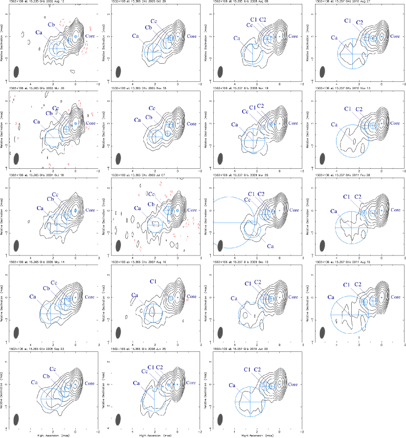
Figure 1: Uniformly weighted, untapered MODELFIT images of PKS 1502+106 at $15$ GHz. Contour levels correspond to $-0.15\%$, $0.15\%$, $0.3\%$, $0.6\%$, $1.2\%$, $2.4\%$, $4.8\%$, $9.6\%$, and $19.2\%$ of the highest peak flux density of $2.79$ Jy/beam (epoch $2009.23$ as listed in Table 3) for common reference. The restoring size is $1.04$ mas $\times$ $0.45$ mas at a position angle of $-6.4^{\circ}$. Labels mark the position of MODELFIT components while unmarked components indicate non-robust features. Time progresses from top to bottom and from left to right.

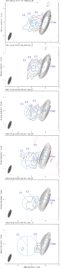
Figure 2: Uniformly weighted, untapered MODELFIT images of PKS 1502+106 at $43$ GHz. Controur levels correspond to $-0.1\%$, $0.1\%$, $0.2\%$, $0.4\%$, $0.8\%$, $1.6\%$, $3.2\%$, $6.4\%$, and $12.8\%$ of the peak flux density of $3.47$ Jy/beam (epoch $2009.35$, see Table 1) for common reference. The restoring beam is shown at the bottom left of each image, with FWHM $0.61$ mas $\times$ $0.19$  mas at a position angle of $-19.9{{}^{\circ}}$. Unmarked components indicate non-robustly identified features.

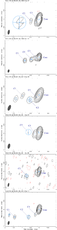
Figure 3: Uniformly weighted, tapered MODELFIT images of PKS 1502+106 at $86$ GHz. Contour levels correspond to $-0.15\%$, $0.15\%$, $0.3\%$, $0.6\%$, $1.2\%$, $2.4\%$, $4.8\%$, $9.6\%$ and $19.2\%$ of the peak flux density of $2.23$ Jy/beam (epoch $2009.35$, see Table 2) as a common reference. The restoring beam is shown at the bottom left of each image. Unmarked components indicate non-robustly identified features.

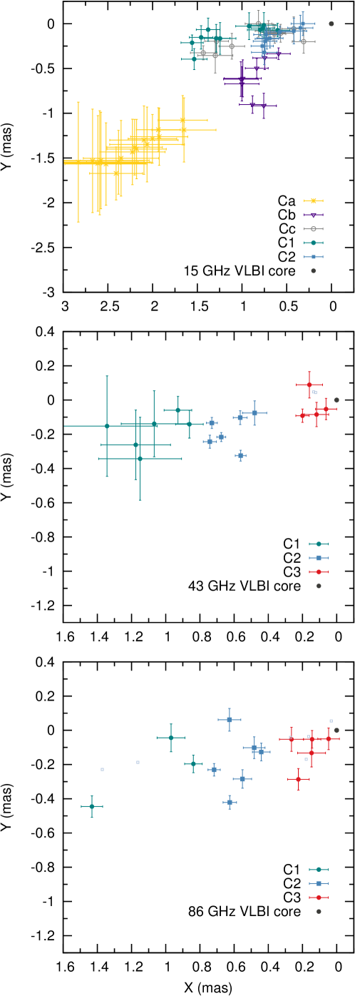
Figure 4: Sky coordinates (relative RA and DEC with respect to the core) of all robustly identified components at $15$, $43$ and $86$ GHz.

3.2 VLBI kinematics at 15, 43, and 86 GHz

To obtain each knot’s proper motion, $\mu$, through the narrow, curved jet of PKS 1502+106 we perform a weighted, linear least-squares fit to their epoch-to-epoch radial separation from the respective core at each frequency. Component radial separations from the core are shown in Fig. 5 for 15, 43, and 86 GHz respectively, where the linear fits are also visible. The inferred values of apparent speed in mas/yr and in units of speed of light ($\beta_{{\rm app}}=\upsilon_{\rm app}/c$), along with ejection dates for all robust jet features are reported in Tables 4, 5, and 6.

Compared to the kinematical results of the MOJAVE program presented in Lister et al. (2013), our component identification is slightly different. It is also based in the cross-identification with the high-frequency data but the overall picture does not differ significantly and knot speeds along with their ejection dates are in very good agreement.

The apparent velocity, $\beta_{\rm{app}}$, of each component is given by:

$$\beta_{{\rm app}}=\dfrac{\mu\,D_{\rm L}}{c(1+z)}$$ (1)

with,

$$\begin{array}[]{lp{0.8\linewidth}}\mu,&the proper motion in rad\,s${}^{-1}$,\\ D_{\rm L},&the luminosity distance in m,\\ c,&speed of light in m\,s${}^{-1}$, and\\ z,&the redshift of the source.\\ \end{array}$$

As evident from Fig. 5 and Tables 4 through 6, PKS 1502+106 is characterized by extremely fast superluminal motion of features within the jet. Measured apparent velocities are in the range of ${\sim}10$ to $22\,c$ at 15 GHz, while at 43 GHz the range is $2$–$11\,c$ and from $7$ to $20\,c$ for 86 GHz. The maximum $\beta_{\rm app}$ per frequency is $\beta_{\rm app}^{\rm 15\,GHz}=(22.1\pm 1.1)$,  $\beta_{\rm app}^{\rm 43\,GHz}=(11\pm 3)$,  $\beta_{\rm app}^{\rm 86\,GHz}=(19.5\pm 0.4)$, all characterizing the motion of superluminal feature C1.

The independently deduced kinematical models per frequency are generally in agreement, with only a few, worthy of discussion discrepancies. These are mainly encountered at our mid-frequency of 43 GHz for components C1 and C2. Here, C1 appears to be traveling downstream the jet with only about half the speed observed at 15 and 86 GHz, where the measurements agree within the observational uncertainties. This is attributed to the large positional uncertainties but also to the small number of high frequency VLBI observations (especially at 43 GHz) which are also limited in $uv$-coverage. Consequently, the absence of even a single data point can drastically affect the quality of the fit and the deduced kinematical parameters.

Inferred apparent component speeds allow for a study of the $\beta_{\rm app}$ profile along the radial direction of the jet. This is presented in Fig. 6. Up to a distance of about $1.5$ mas from the core the apparent speeds observed, follow an almost monotonically increasing trend, peaking at about 1 mas at all frequencies. Beyond 1.5 mas downstream, the trend seems to break with only one, though robust, measurement at 15 GHz for the historical component Ca having only a $\beta_{\rm app}=(9.7\pm 1.2)$ at a radial separation of ${\sim}2.8$ mas, indicating a change of physical conditions within the flow – e.g. deceleration and/or change of the viewing angle. In the immediate vicinity of the core, knot C3 moves outwards with an apparent superluminal speed of $(5.0\pm 3.7)\,c$ and $(7.1\pm 0.7)\,c$, at 43 and 86 GHz respectively.

The XY (RA–DEC) position and the radial separation plots presented in Fig. 4 and 5 reveal the erratic path of superluminal feature C2 both at 43 and 86 GHz. The emerging pattern is not inconsistent with, and could in fact hint towards, the scenario that C2 is following a helical trajectory. A scenario though, that cannot be corroborated due to the limited number of observations and the consequently low sampling rate of the underlying motion.

Other physical effects may also contribute to small, observed differences. For example, the small angles under which blazars are viewed, having the potential of greatly magnifying relativistic aberration effects and the position of the core itself which can constitute a non-stationary feature, subject to erratic motion. However, such an effect in not clearly seen by the motion of other superluminal components. An additional effect, as resolution increases, is that more compact regions are picked up by the interferometer, thus shifting the centroid of a fitted component within a larger emission region (as seen at lower frequencies).

For those jet components that can be identified across observing frequencies, ejection dates are again in good agreement, with the exception of C2 whose wobbly motion does not allow a good estimation of the ejection date at 43 GHz. Components C1, C2 and C3 have been separated from the core in the time period covered by the VLBI monitoring. C1 and C2 were ejected between 2005 and 2006, while C3 in ${\sim}2008$, at a time close to the onset of the multi-frequency outburst of PKS 1502+106.

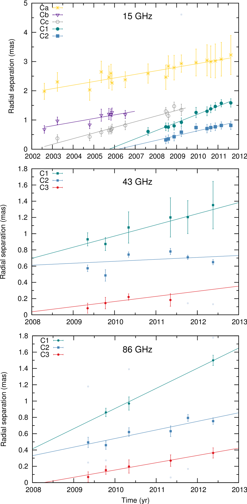
Figure 5: Temporal evolution of component radial separation from the core at – from top to bottom – $15$, $43$, and $86$ GHz. While the long-term kinematical behavior of PKS $1502{+}106$ is visible at the lowest frequency, $43$ and $86$ GHz observations allow for a high resolution view towards the inner jet of PKS $1502{+}106$. Components C1 and C2 identified across all frequencies can be seen using the same color code.

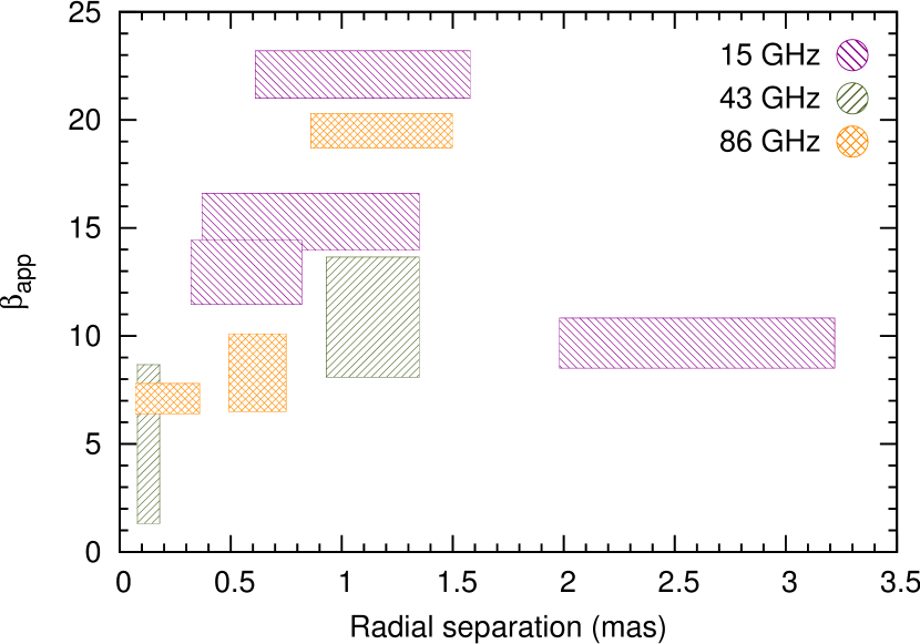
Figure 6: Apparent speed profile of superluminal components as a function of radial separation from the core. The vertical extent of rectangles represents the uncertainty in $\beta_{\rm app}$. Their horizontal extent denotes the distance that each component has traversed within the jet, during the monitoring period. A rising trend is seen up to a projected separation of ${\sim}$1.6  mas, after which a lower apparent speed is seen.

Table 4: Derived kinematical parameters of jet components at $15$ GHz

Knot	$\mu$	$\beta_{\rm app}$	$t_{\rm ej}$
	$({\rm mas\,yr^{-1}})$	($c$)	(yr)
Ca	$0.122\pm 0.015$	$\leavevmode\nobreak\ \leavevmode\nobreak\ 9.7\pm 1.2$	$1986.1\pm 2.6$
Cb	$0.125\pm 0.033$	$\leavevmode\nobreak\ \leavevmode\nobreak\ 9.8\pm 2.6$	$1996.6\pm 2.2$
Cc	$0.193\pm 0.017$	$15.3\pm 1.3$	$2002.1\pm 0.4$
C1	$0.280\pm 0.014$	$22.1\pm 1.1$	$2005.7\pm 0.2$
C2	$0.164\pm 0.019$	$13.0\pm 1.5$	$2006.2\pm 0.5$

Table 5: Derived kinematical parameters of jet components at 43 GHz

Knot	$\mu$	$\beta_{\rm app}$	$t_{\rm ej}$
	$({\rm mas\,yr^{-1}})$	($c$)	(yr)
C1	$0.138\pm 0.035$	$10.9\pm 2.8$	$2003.0\pm\leavevmode\nobreak\ \leavevmode\nobreak\ 2.0$
C2	$0.024\pm 0.035$	$\leavevmode\nobreak\ \leavevmode\nobreak\ 2.0\pm 2.7$	$1982.5\pm 41.5$
C3	$0.063\pm 0.047$	$\leavevmode\nobreak\ \leavevmode\nobreak\ 5.0\pm 3.7$	$2007.4\pm\leavevmode\nobreak\ \leavevmode\nobreak\ 2.2$

Table 6: Derived kinematical parameters of jet components at 86 GHz

Knot	$\mu$	$\beta_{\rm app}$	$t_{\rm ej}$
	$({\rm mas\,yr^{-1}})$	($c$)	(yr)
C1	$0.247\pm 0.010$	$19.5\pm 0.8$	$2006.3\pm 0.2$
C2	$0.105\pm 0.023$	$\leavevmode\nobreak\ \leavevmode\nobreak\ 8.3\pm 1.8$	$2004.9\pm 1.4$
C3	$0.090\pm 0.009$	$\leavevmode\nobreak\ \leavevmode\nobreak\ 7.1\pm 0.7$	$2008.3\pm 0.3$

3.3 Radio flux density decomposition

The flare in PKS 1502+106 is dominated by a single, clearly visible event from $\gamma$-ray energies down to radio frequencies, between MJD $54689$ and MJD $55295$. The upper panel of Fig. 7 features the Fermi/LAT $\gamma$-ray light curve and following panels depict the total intensity radio data, both from the filled-aperture F-GAMMA observations and from cm/mm-VLBI monitoring. The total, single-dish flux density is decomposed into individual VLBI core and jet-component light curves. We show those of the positively cross-identified components C1, C2, and C3, omitting the historical components, at 15 GHz, and any non-robust jet features.

The core dominates the total flux density at VLBI scales at all frequencies. Radio flux density decomposed into core and MODELFIT components accounts for the largest fraction of the total single-dish flux density and follows nicely the flare evolution. Only in few cases, the sum of flux density of all MODELFIT components deviates from the total single-dish flux density. This is attributed to the low cadence of mm-VLBI monitoring and the source’s extreme variability behavior. The presence of substructure in the well-sampled F-GAMMA and $\gamma$-ray light curves provides evidence for such fast variability.

Our mm-VLBI monitoring reveals that the radio flare, for its whole duration, is dominated by emission from the core, which at 15 GHz has varied in flux density by a factor of $\sim$3 with a time scale of approximately 2 years (see Fig. 7). The same behavior persists also at 43 and 86 GHz where its flux density varies by a factor of $\sim$6–7 and $\sim$4–5, respectively, within our GMVA monitoring period.

At 43 and 86 GHz, where resolution allows, it is clear that the flare is not an attribute of the core only. Here, the most recently ejected component C3 appears to be in a decaying phase already during the first mm-VLBI observing epoch, but still shows significantly higher flux densities compared to all later epochs (see middle panels of Fig. 7 and Fig. 12). Despite the limited number of data for C3, it can be clearly seen that – apart form the core – it is the only moving jet feature that is flaring, with its flux density dropping by a factor of ${\sim}20$, at both frequencies. For completeness, all individual component light curves are shown in the Appendix.

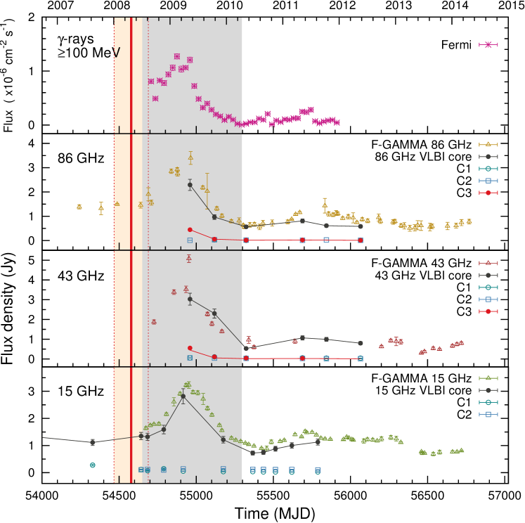
Figure 7: Light curves of PKS $1502{+}106$. From top to bottom are shown: the monthly-binned Fermi/LAT $\gamma$-ray light curve at energies $E>100$ MeV; F-GAMMA single-dish radio light curve at $86$ GHz with the core and component light curves from the VLBI flux density decomposition; same as before but at $43$ GHz and (lower panel) at $15$ GHz. Note the VLBI knot C3, only visible at the two highest frequencies, at its decaying flux density phase. The gray shaded area delineates the full duration of the flare ${\sim}650$ days. The red shaded area marks the estimated ejection interval of knot C3 with the red solid line designating its $t_{\rm ej}$.

3.4 Spectra of individual knots

While our high-frequency GMVA data at 43 and 86 GHz are concurrent, this is not the case for the 15 GHz VLBA data. In order to assemble quasi-simultaneous spectra of individual superluminal components within the jet of PKS 1502+106, we select the 15 GHz epochs closest in time to each of the six 43/86 GHz GMVA observing runs. The quasi-simultaneous data forming each of the six spectra are labeled, I to VI, in Tables 1 through 3. Assembled spectra are shown in Fig. 8. The mean separation between the 15 GHz and 43/86 GHz observing epochs composing them is ${\sim}51$ days.

Components C1 and C2 are positively cross-identified between all three observing frequencies (Sect. 3.1) and hence quasi-simultaneous spectra were assembled for those. Knot C1 is the only sufficiently sampled component that shows evidence of a synchrotron self-absorbed spectrum (SSA) featuring a spectral break at the turnover frequency, $\nu_{\rm m}$ and flux density $S_{\rm m}$. In order to obtain $S_{\rm m}$ and $\nu_{\rm m}$, along with the optically-thin spectral index we fit a model SSA spectrum of the following form (e.g. Türler et al., 2000):

$$S_{\nu}=S_{\rm m}\left(\dfrac{\nu}{\nu_{\rm m}}\right)^{\alpha_{\rm t}}\dfrac{1-\exp[-\tau_{\rm m}(\nu/\nu_{\rm m})^{\alpha-\alpha_{\rm t}}]}{1-\exp(-\tau_{\rm m})}$$ (2)

where:

$$\begin{array}[]{lp{0.8\linewidth}}\nu_{\rm m},&is the turnover frequency in\,GHz,\\ S_{\rm m},&is the turnover flux density in Jy,\\ \tau_{\rm m},&$\sim 3/2\left(\sqrt{1-\dfrac{8\alpha}{3\alpha_{\rm t}}}-1\right)$ is the optical depth at $\nu_{\rm m}$,\\ \alpha_{\rm t},&is the spectral index of the optically thick part of the emission, and\\ \alpha,&is the optically-thin spectral index.\\ \end{array}$$

The spectral index for the optically thick part is fixed to the canonical value $\alpha_{\rm t}=5/2$. We fit the observed spectra of C1 simultaneously and obtain $S_{\rm m}=(0.08\pm 0.01)$ Jy, $\nu_{\rm m}=(33.2\pm 2.0)$ GHz and $\alpha=-(2.5\pm 0.4)$, as the average spectral index. The spectral index characterizing knot C1 is arguably very steep. This could indicate that the component at the highest frequency is resolved-out, as a result of high resolution (i.e. small observing beam), leading to an underestimation of its flux density. An additional uncertainty in $\alpha$ of up to 15% is also to be expected, arising from the different $uv$-coverages (e.g. Fromm et al., 2013). To obtain the same parameters during the highest state of the knot, the fit is performed once more, at epoch 2009.9 only. Resulting parameters are as follows: $S_{\rm m}=0.133$ Jy, $\nu_{\rm m}=36.7$ GHz and $\alpha=-1.98$. These were used for the calculation of the magnetic field from SSA in Sect. 4.5.

For components C2 and C3 showing no sign of a SSA break, a power-law fit is performed separately at each observing epoch and the mean optically thin spectral index $\left<\alpha\right>$, characterizing the time-averaged spectrum, along with its standard error are reported in Table 7.

C2 is also a well-sampled feature that during the whole length of our VLBI monitoring is characterized by a steep optically-thin spectrum with a mean power-law index of $\left<\alpha\right>=-(1.0\pm 0.3)$ and a peak at ${\leq}15$ GHz. However, the situation is less constrained for component C3 that is only seen at $43$ and $86$ GHz due to the resolution limit of the $15$ GHz observations. Here, the analysis yielded an optically-thin, two-point spectral index $\left<\alpha\right>=-(0.8\pm 0.3)$.

The core is the most compact, stationary feature at each frequency and it is characterized by a flat spectrum; i.e. $\alpha\geq-0.5$. However, at epoch $2009.9$ it appears to exhibit a SSA turnover at $\nu_{\rm m}\sim 43$ GHz. The mean spectral index of the core is found to be $\left<\alpha\right>=-(0.22\pm 0.07)$, indicative of unresolved substructure.

Table 7: Spectral indices for components C1, C2, C3, and the core as obtained by SSA fitting for C1 and a single power-law fit for C2 and C3.

Knot	$\left<\alpha\right>$
C1	$-2.5\pm 0.4$
C2	$-1.0\pm 0.3$
C3	$-0.8\pm 0.3$
Core	$-0.22\pm 0.07$

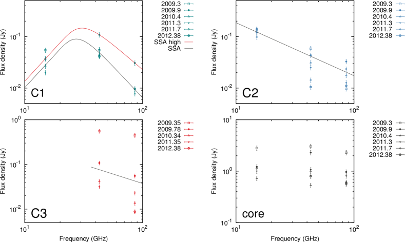
Figure 8: Three-point spectra of knots C1, C2, the VLBI core and their temporal evolution. For C3 spectra are only available at $43$ GHz and $86$ GHz since it is blended at $15$ GHz. Black lines represent the time-averaged spectra of components and their slopes are reported in Table 7. For component C1 the fitted SSA model spectra are also shown. The red curve is a SSA fit during its highest state, while the black corresponds to the mean SSA spectrum.

4 Inferred physical parameters

In the present section, we deduce physical parameters of the jet of PKS 1502+106, given the phenomenological characteristics presented in Sect. 3. We discuss the Doppler factor, viewing angle, and brightness temperature distribution along the jet, and estimate magnetic field strengths.

4.1 Doppler and Lorentz factor estimates

As shown in Sect. 3.2, the highest apparent speed measured in the jet of PKS 1502+106 is $\beta_{\rm app}\sim 22$ and corresponds to that of component C1 at 15 GHz. From here we can readily estimate the minimum Lorentz factor that characterizes the flow (see for example the review by Urry & Padovani, 1995). It follows that $\gamma\geq\gamma_{\rm min}$ for the jet with the minimum Lorentz factor given by

$$\gamma_{\rm min}=\sqrt{\beta_{\rm app}^{2}+1},$$ (3)

and for the observed maximum apparent velocity we obtain $\gamma_{\rm min}=22.1$. Consequently, if the jet is viewed at the critical angle (see Sect. 4.2), Doppler factors can be estimated too, since $\delta_{\beta_{\rm app},\,C1}\sim\beta_{\rm app,\,C1}=22.1$ at 15 GHz. For knots C2 and C3, it is $\delta_{\beta_{\rm app}}\sim\gamma_{\rm min,\,C2}=9.3$ and $\delta_{\beta_{\rm app}}\sim\gamma_{\rm min,\,C3}=7.2$, from the 86 GHz observations.

In addition to the Doppler factor estimate obtained from the minimum Lorentz factor, under the valid assumption of causality one can arrive to another estimate of the Doppler factor, $\delta_{\rm var}$, using the temporal variation of the flux density of individual components. For details on this method and for a full derivation see Jorstad et al. (2005) and Onuchukwu & Ubachukwu (2013), respectively. The variability Doppler factor is given by

$$\delta_{\rm var}=\dfrac{d_{{\rm eff}}\,D_{\rm L}}{c\Delta t_{{\rm var}}\,(1+z)},$$ (4)

where:

$$\begin{array}[]{lp{0.8\linewidth}}d_{{\rm eff}},&is the effective angular size of the component in rad and\\ \Delta t_{\rm var},&the variability time scale, $[{=}dt/\ln(S_{\rm max}/S_{\rm min})]$, with $dt$ the time between $S_{\rm max}$ and $S_{\rm min}$\\ \end{array}$$

Components C1 and C3 can be used for this purpose. Both components are unresolved; that is, being smaller than the beam size at the epoch of their highest respective flux densities at all three observing frequencies. In all cases (for C1 at 15 GHz and for C3 at 43 and 86 GHz) we have used the minor axis of the restoring beam as the upper limit for the component angular size. This selection is based on the fact that the minor axis is positioned almost parallel to the jet axis, thus allowing the highest resolution to be achieved along it. Specifically, for the higher frequencies and component C3 the minor axis of the 86 GHz beam was selected, since it yields the most stringent upper limit to its size.

A simple inspection of the light curves indicates that component flux density variations are not adequately sampled, while the point of maximum flux density most probably precedes our first observing epoch. Nevertheless, based on the comparison with the single-dish data (Sect. 3.3), this point cannot be too displaced (in time), nor much higher (in flux density) from the first data point in the mm-VLBI light curves. We therefore employ the method, since useful nominal values can be obtained. We calculate $\Delta t_{\rm var}$, with $dt$ and $S_{\rm max}$ obtained directly from the light curves of individual components.

Along the same argumentation an estimate of the Lorentz factor can be obtained by

$$\gamma_{\rm var}=\dfrac{\beta_{\rm app}^{2}+\delta_{\rm var}^{2}+1}{2\delta_{\rm var}}.$$ (5)

Results of the calculations are summarized in Table 8. Component C1 is characterized by the highest variability Doppler ($\delta_{\rm var}\sim 51.4$) and Lorentz ($\gamma_{\rm var}\sim 30.5$) factors. All figures are consistent with the estimates of the minimum Lorentz factor, $\gamma_{\rm min}$, presented previously. Knot C3 is also found to have consistent behavior at both high frequencies with $\delta_{\rm var}^{\rm 43\,GHz}\sim 12.1$ and $\gamma_{\rm var}^{\rm 43\,GHz}\sim 7.1$, while at $86$ GHz the estimation yields $\delta_{\rm var}^{\rm 86\,GHz}\sim 15$ and $\gamma_{\rm var}^{\rm 86\,GHz}\sim 9.2$.

An additional Doppler factor estimate can be obtained from the relative strength of the synchrotron self-absorption and equipartition magnetic fields. This is discussed in Sect. 4.5.

Table 8: Physical parameters estimated using variability arguments.

Knot	$\nu$	$dt$	$d_{\rm eff}$	$\Delta t_{\rm var}$	$\delta_{\rm var}$	$\gamma_{\rm var}$	$\theta_{\rm var}$
	(GHz)	(yr)	(mas)	(yr)			(∘)
C1	15	3.6	${\leq}0.9$	$1.3$	$51.4$	$30.5$	$0.8$
C3	43	1.9	${\leq}0.1$	$0.7$	$12.1$	$7.1$	$3.4$
C3	86	1.9	${\leq}0.1$	$0.7$	$15.0$	$9.2$	$2.9$

4.2 The viewing angle towards PKS 1502+106

Using the observed apparent speed we can set constraints to the aspect angle under which a jet is viewed in two ways.

First, by calculating the critical angle which results in the observed $\beta_{\rm app}$ with the minimum $\gamma$. The apparent speed is given by (Rees, 1966)

$$\beta_{\rm app}=\dfrac{\beta\sin\theta}{1-(\beta\cos\theta)},$$ (6)

where $\beta$ is the intrinsic velocity in units of $c$ and $\theta$ is the viewing angle. Using the definition of the Doppler factor, $\delta=[\gamma(1-\beta\cos\theta)]^{-1}$, Eq. 6 can be rewritten as

$$\beta_{\rm app}=\beta\gamma\delta\sin\theta,$$ (7)

and $\beta_{\rm app}$ is maximized (i.e. $\beta_{\rm app,\,max}=\beta\gamma$) for $\sin\theta_{\rm c}=\gamma^{-1}$ or $\sin\theta_{\rm c}=\delta^{-1}$, since for this angle $\theta_{\rm c}$, $\gamma=\delta$. With the minimum Lorentz factor, $\gamma_{\rm min}=22.1$, calculated above we arrive to the following figure for the critical angle:

$$\theta_{\rm c}=\arcsin\left(\dfrac{1}{\gamma_{\rm min}}\right)=2.6^{\circ}.$$ (8)

We can also estimate the viewing angle towards the source, based on causality arguments. This “variability viewing angle”, $\theta_{\rm var}$, is given by

$$\theta_{\rm var}=\arctan\left(\dfrac{2\beta_{\rm app}}{\beta_{\rm app}^{2}+\delta_{\rm var}^{2}-1}\right).$$ (9)

This analysis was performed for two components with significant variability (see Fig. 12) and yields viewing angles for each component separately. The results are shown in the last column of Table 8. For the fastest superluminal knot, C1, we obtain the smallest viewing angle $\theta_{\rm var}\sim 0.8^{\circ}$. For C3 we obtain consistent values at $43/86$ GHz of ${\sim}3.4^{\circ}$ and ${\sim}2.9^{\circ}$, respectively.

Interestingly, components C1 and C3 are traveling with very different apparent speeds (Sect. 3.2) at two different regions of the jet – i.e. in the outer ($r>1$ mas) and inner jet ($r<0.5$ mas), respectively. This fact, in combination with the difference of their inferred Doppler factors hints towards a “two-region scenario”, wherein physical conditions are intrinsically different. This possibility is further discussed in the following.

4.3 Opening angle of the jet

In the present section we investigate the apparent and intrinsic opening angles of the jet, $\phi_{\rm app}$ and $\phi_{\rm int}$, respectively employing two different approaches. First, we use all MODELFIT components at all three frequencies, and perform a simultaneous linear fit to their sizes in order to obtain the jet opening rate. In the second approach we deduce $\phi_{\rm app}$ from each individual MODELFIT component based on its size and kinematical characteristics.

4.3.1 The $\phi_{\rm int}$ from simultaneously fitting the effective sizes

In Fig. 9 the effective deconvolved size, $d_{{\rm eff}}=1.8\,\mbox{FWHM}_{\rm d}$ with $\mbox{FWHM}_{\rm d}=\left(\mbox{FWHM}^{2}-b_{\phi}^{2}\right)^{1/2}$, of all resolved MODELFIT components at all three frequencies is shown as a function of radial separation from the core. The factor 1.8 accounts for the fact that a Gaussian with FWHM equal to $d$, roughly corresponds to a circle of angular diameter $1.8\,d$. We fit $d_{{\rm eff}}$ with respect to radial separation from the core, using a simple linear model assuming a constant jet opening angle. The least-squares fit yields a slope of $\left(1.7\pm 0.1\right)$ translating to an apparent half-opening angle of $(40.4\pm 1.7)^{\circ}$ and an apparent full-opening angle of $\phi_{{\rm app}}=(80.8\pm 3.4)^{\circ}$. The de-projected opening angle is then given by

$$\phi_{\rm int}=\phi_{\rm app}\,\sin\theta,$$ (10)

which for $\theta=\theta_{\rm c}=2.6^{\circ}$ (see Sect. 4.2) yields $\phi_{\rm int}=(3.7\pm 0.2)^{\circ}$.

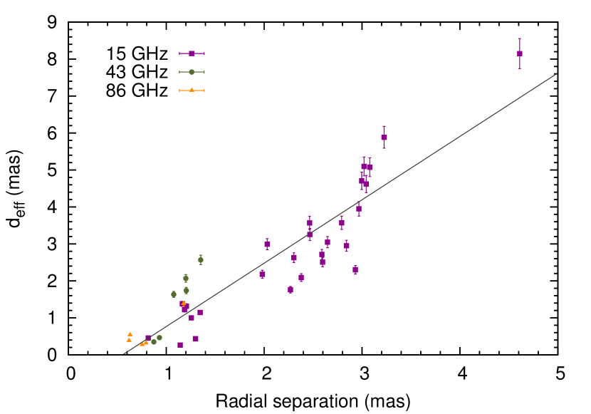
Figure 9: Effective deconvolved size of all resolved jet components with respect to radial separation from the core, at all frequencies. A line represents the best fit to the data.

4.3.2 The $\phi_{\rm int}$ from individual knots

We performed the analysis on the $uv$-plane, utilizing the component size, ${\rm FWHM}_{\rm d}$, and radial distance, $r$, from the core. First, we calculate the opening angle corresponding to each MODELFIT component separately. Assuming the component filling the entire jet cross section, $\phi_{\rm app}$ is given by

$$\phi_{\rm app}^{\rm comp}=2\arctan\left(\dfrac{1.8\,{\rm FWHM}_{\rm d}}{2r}\right).$$ (11)

Then, we average over effective size and distance, thus obtaining the average opening angle of a given component at a mean radial separation from the core. The intrinsic opening angle of the jet, making use of the critical viewing angle for each component, is given by Eq. 10. The results are shown in Table 9. The mean intrinsic opening angle for the jet, deduced by averaging the $\left<\phi_{\rm int}\right>$ of all components is $(3.9\pm 1.0)^{\circ}$.

Table 9: Apparent and intrinsic jet opening angles deduced from individual MODELFIT components.

Knot	$\nu$	Epochs	$\left<r\right>$	$\theta_{\rm c}$	$\left<\phi_{\rm app}\right>$	$\left<\phi_{\rm int}\right>$
	(GHz)		(mas)	(∘)	(∘)	(∘)
Ca	15	19	2.6	5.9	63.7	6.5
Cb	15	3	1.2	5.8	57.7	5.8
Cc	15	3	1.1	3.8	30.2	2.0
C1	15	2	1.3	2.6	31.3	1.4
C1	43	6	1.1	6.2	60.9	6.6
C2	86	4	0.7	2.9	31.0	1.6

4.4 Radial distribution of the brightness temperature

The apparent brightness temperature of a given VLBI component in the source rest frame is given by:

$$T_{\rm b}=1.22\times 10^{12}\,\dfrac{S_{\nu}}{\nu^{2}\,d_{{\rm eff}}^{2}}\,(1+z)\leavevmode\nobreak\ \leavevmode\nobreak\ \leavevmode\nobreak\ \leavevmode\nobreak\ (K),$$ (12)

where:

$$\begin{array}[]{lp{0.8\linewidth}}S_{\nu},&is the component's flux density in Jy,\\ d_{{\rm eff}},&the effective size of the emitting region in mas, and\\ \nu,&the observing frequency in GHz.\\ \end{array}$$

In Fig. 10, we present the radial distribution of brightness temperatures along the jet of PKS 1502+106. The $T_{\rm b}$ is frequency-dependent, with higher values at the lowest frequencies. Observed brightness temperatures approach and mostly exceed the equipartition limit (Readhead, 1994) of about $5\times 10^{10}$ K for the core, at all frequencies (see Fig. 10). The core is at all times unresolved and thus the $T_{\rm b}$ values represent lower limits. The same trend of high $T_{\rm b}$ persists throughout the first mas downstream of the core, with a few components being resolved. Specifically, in the regions

• between $0$ and $1$ mas, high $T_{\rm b}$ is seen at all frequencies, evidenced from lower limits, with a handful of measured values of lower $T_{\rm b}$, as observing frequency increases. Those lie in the range from $10^{7}$ K at 86 GHz, to slightly above $10^{9}$ K at 15 GHz.

• Between $1$ and $2$ mas, the division persists, indicative of the sampling of different portions of the jet. Here the measurements at 15 GHz are clustered in the range $10^{9}$–$10^{10}$ K at 15 GHz, while at both high frequencies the $T_{\rm b}$ is significantly lower, $T_{\rm b}\geq 10^{7}$ K.

• Beyond $2$ mas, the jet is observable only at 15 GHz and the distribution of $T_{\rm b}$ is characterized by a decreasing trend from $10^{9}$ K to $10^{8}$ K at a distance of $4.6$ mas.

The mean – over time – core brightness temperature at our three observing frequencies is: $\left<T_{\rm b,\,core}^{\rm 15\,GHz}\right>\geq(3.8\pm 1.5)\times 10^{10}$ K, $\left<T_{\rm b,\,core}^{\rm 43\,GHz}\right>\geq(1.5\pm 1.0)\times 10^{10}$ K, and $\left<T_{\rm b,\,core}^{\rm 86\,GHz}\right>\geq(7.4\pm 5.0)\times 10^{9}$ K.

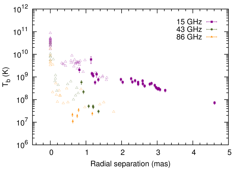
Figure 10: Brightness temperature, $T_{\rm b}$, versus the radial separation from the core at all observing frequencies indicated by the color code. Filled symbols represent $T_{\rm b}$ measurements, while open triangles represent lower limits at all frequencies.

4.5 Magnetic field estimates

Estimates of the magnetic field strength for individual components can be obtained under the assumption that synchrotron self-absorption (SSA) is the dominant process shaping the observed spectra. Following Marscher (1983) the strength of the magnetic field can then be calculated as

$$B_{{\rm SSA}}=10^{-5}b(a)\,\vartheta^{4}\nu_{\rm m}^{5}S_{\rm m}^{-2}\left(\dfrac{\delta}{1+z}\right)\leavevmode\nobreak\ \leavevmode\nobreak\ \leavevmode\nobreak\ \leavevmode\nobreak\ (G),$$ (13)

where:

$$\begin{array}[]{lp{0.8\linewidth}}b(a),&is a tabulated spectral index-dependent parameter \cite[cite]{(cf. \@@bibref{AuthorsPhrase1Year}{1983ApJ...264..296M}{\@@citephrase{, }}{}, Table 1)}\\ \vartheta,&the component size in mas\\ \nu_{\rm m},&the spectral turnover frequency in GHz, and\\ S_{\rm m},&the spectral turnover flux density in Jy.\end{array}$$

Given the strong dependencies of $B_{{\rm SSA}}$, mainly on $\nu_{\rm m}$ and $\vartheta$, we note that measurement uncertainties of those quantities, translate into large uncertainty of $B_{{\rm SSA}}$, as given by Eq. 13. Nevertheless, we attempt the estimation for those components that the turnover frequency and flux density are somewhat constrained, namely knot C1 and the core. Even if a Doppler factor $\delta$, correction is not applied, an apparent value along the jet can be obtained (Bach et al., 2005). Table 10 summarizes our findings.

C1 exhibits a strong magnetic field of ${\sim}5.0\delta$ G. This large value could be an indication of a highly-magnetized disturbance traveling along the jet. Its high apparent velocity of $22.1\,c$ and high Doppler factor ($22.1\leq\delta\leq 51.4$) hint towards this scenario.

The characteristic spectral flatness of the core is traditionally attributed to the superposition of a number of individual SSA components, each with a distinctly peaked spectrum. The spectral shape of the core at epoch $2009.9$ (see Fig. 8) hints the presence of a SSA peak close to a frequency of ${\sim}43$ GHz. Taking this as the turnover frequency and with $S_{\rm m}=2.3$ Jy we obtain a SSA magnetic field of $B_{{\rm SSA}}\sim 2\delta$ mG.

Table 10: Estimated physical parameters for knot C1 and the core.

Knot	$\nu_{\rm m}$	$S_{\rm m}$	$\vartheta$	$B_{\rm SSA}/\delta$	$B_{\rm eq}$	$\delta_{\rm eq}$
	(GHz)	(Jy)	(mas)	(G)	(G)
C1	$36.7$	$0.13$	$0.10$	$5.0$	$0.3$	${\sim}50$
Core	${\sim}43$	$2.3$	$0.06$	$0.002$	$1.2$	…

Another constraint to the magnetic field can be set assuming equipartition between the energy of radiating relativistic particles ($E_{e}\propto B^{-1.5}$) and that of the magnetic field ($E_{B}\propto B^{2}$). The equipartition magnetic field that minimizes the total energy content $E_{\rm tot}=(1+k)E_{e}+E_{B}$ is (see e.g. Bach et al., 2005)

$$B_{\rm eq}=\left[4.5\,(1+k)\,f(a,\nu_{\rm a},\nu_{\rm b})\,L\,R^{3})\right]^{2/7}$$ (14)

where:

$$\begin{array}[]{lp{0.8\linewidth}}k,&is energy ratio between electrons and heavy particles,\\ f,&is a tabulated function of $\alpha$, and upper and lower synchrotron frequency cutoffs, $\nu_{\rm a}$, $\nu_{\rm b}$ in\,GHz\\ L,&is the synchrotron luminosity of the source given by $L=4\pi D_{\rm L}^{2}\int_{\nu_{\rm a}}^{\nu_{\rm b}}Sd\nu$, and\\ R,&is the size of the knot in cm.\end{array}$$

For $k\sim 100$ and $f(-0.5,10^{7},10^{11})=1.6\times 10^{7}$, we obtain the following expression

$$B_{\rm eq}=5.37\times 10^{12}\,(S_{\rm m}\nu_{\rm m}D_{\rm L}^{2}R^{-3})^{2/7}.$$ (15)

Knot C1 is characterized by an equipartition magnetic field of about $0.3$ G and the core features the highest equipartition magnetic field, $B_{\rm eq}\sim 1.2$ G. Results are shown in Table 10.

The two magnetic field estimates have a different dependence on the Doppler factor. On the one hand, $B_{\rm SSA}\propto\delta$ for the magnetic field strength calculated from SSA, and $B_{\rm eq}\propto\delta^{(2/7\alpha+1)}$ for the minimum, equipartition magnetic field. We use those to get an estimate of $\delta_{\rm eq}$, when possible, from the ratio $B_{\rm eq}/B_{\rm SSA}=\delta_{\rm eq}^{2/7\alpha}$. The estimated equipartition Doppler factor for C1, $\delta_{\rm eq,\,C1}\sim 50$, is also in good agreement with $\delta_{\rm var}\sim 51.4$. Given the assumptions, all values are in reasonable agreement.

5 Discussion

5.1 The $\gamma$-ray/radio flare

The Fermi/LAT light curve, adopted from Fuhrmann et al. (2014) and shown in Fig. 7 (top panel), spans the time period between MJD $54707$ (2008.66) through MJD $55911$ (2011.96). The source is already at high state, since the beginning of our monitoring period. From then on, the rising trend continues until MJD $54875$ (2009.12), when the absolute maximum in the monthly averaged $\gamma$-ray photon flux (of ${\sim}1.3\times 10^{-6}\,{\rm cm^{-2}\,s^{-1}}$), is reached. In fact, there exists some amount of sub-structure in the $\gamma$-ray light curve. A second – this time local – maximum is reached on MJD $54959$ (2009.35) with comparable flux. Altogether, activity at high energies, from its start until the first – and absolute – minimum is reached on MJD $55295$ (2010.27), lasts for almost 650 days (shaded area in Fig. 7).

In Savolainen et al. (2002), a general connection between radio outbursts and newly ejected jet features has been made, with most radio flares accompanied by the ejection of one or more components. While usually the brightness of knots associated with $\gamma$-ray/radio flares decays fast, here we follow the evolution of one thanks to the enhanced resolution of mm-VLBI. As discussed in Sect. 3.3 apart from the flaring VLBI core, component C3 visible at 43 and 86 GHz only, is characterized by a decaying light curve with an initial flux density level – at epoch 2009.35 – almost 10 times higher than that of the other two components (C1, C2) present in the flow and seen also at both high frequencies. Although a certain amount of flux density blending between the core and C3 is plaussible, we note the relatively high spatial separation of the two components (approximately one beam at 86 GHz in 2009.35) and the high signal-to-noise ratio of C3. These two facts add to the argument that C3 is indeed flaring/decaying, in addition to the flaring core.

Our observations are consistent with C3 having an apparent speed of $7.1\,c$ (Sect. 3.2) and its ejection year, based on the kinematical models at 43 GHz and 86 GHz, is ($2007.4\pm 2.2$) and ($2008.3\pm 0.3$), respectively. C3’s time of zero separation (red solid line in Fig. 7) coincides with the onset of the $\gamma$-ray flare when extrapolating the rate of $\gamma$-ray flux change, as it rises linearly, back in time. We conclude, based on the ejection date of superluminal component C3, that it is most probably associated with the $\gamma$-ray flare and its radio counterpart. Since its separation from the core, it is traveling downstream the jet with an apparent superluminal velocity (see Table 6). We note the larger uncertainty in the knot’s time of ejection at 43 GHz as compared to observation at 86 GHz. That is due to the sparser sampling at this frequency and the higher impact to the fit due to the very last data point in the radial separation plot (middle panel of Fig. 5). In any case, the two figures are consistent with each other. Assuming the speed of knot C3 to remain constant, at the times of the two $\gamma$-ray photon flux maxima, in 2009.2 and 2009.4 (at MJD 54897 and 54959) the knot is at a projected distance of ${\sim}0.7$ and ${\sim}0.8$ pc downstream the 3-mm core, respectively.

A plausible scenario is that a disturbance originating at the jet nozzle of PKS 1502+106, while still upstream of the 3 mm core – i.e. the unit-opacity surface at 86 GHz – produces the observed $\gamma$-ray emission. As it continues to move outwards, it becomes optically thin while crossing the 3-mm VLBI core hence producing the radio flare. Alternatively, the core may represent the first conical recollimation shock of the flow (Daly & Marscher, 1988; Gómez et al., 1995; Bogovalov & Tsinganos, 2005; Marscher, 2008), in which case the flare can be attributed to shock–shock interaction and subsequent enhancement of emission. In both cases, as the disturbance moves further downstream, is observed as knot C3 at its decaying flux density phase.

5.2 Distance estimates to the central engine

The debate as to where in the jet the high-energy emission originates, is presently far from being considered resolved. In this paper, combining radio single-dish monitoring data and our findings from the VLBI analysis of PKS 1502+106, we explore and further constrain the region where the pronounced MeV/GeV activity of 2009 takes place and compare with the SED modeling results of Abdo et al. (2010).

Under the assumption that the core takes up the entire jet cross section and for a constant opening angle, the de-projected distance of the 86 GHz core from the vertex of the hypothesized conical jet can be estimated using the following expression

$$d_{\rm core}=\dfrac{1.8\,\left<\mbox{FWHM}_{\rm core}\right>}{2\,\tan(\phi_{\rm int}/2)}.$$ (16)

With an average size for the core $\left<\mbox{FWHM}_{\rm core}\right>=0.03$ mas and a nominal opening angle $\phi_{\rm int}=(3.8\pm 0.5)^{\circ}$ (Sect. 4.3), the 86 GHz core is constrained to a distance of $d_{\rm core}\leq 8$ pc away from the jet base. This figure takes into account the uncertainty in $\phi_{\rm int}$. Here, $d_{\rm core}$ is an upper limit, as the core is at all times unresolved, rendering $\mbox{FWHM}_{\rm core}$ an upper limit to its angular size.

In an effort to detect and assess possible correlations between radio and $\gamma$ rays, Fuhrmann et al. (2014) apply a cross-correlation function analysis between the single-dish radio light curves at 86 GHz, and the Fermi $\gamma$-ray light curves of 54 blazars from the F-GAMMA sample. Radio emission is typically found to lag behind the activity in $\gamma$ rays. More specifically, for PKS 1502+106, statistically significant correlation is found between the two bands (see light curves in Fig. 7). Radio lags $\gamma$ rays by $14\pm 11$ days at a significance level above 99%. Using Eq. 3 in the same paper, this time lag translates into a distance of $2.1$ pc upstream of the $\tau=1$ surface at 86 GHz, for the $\gamma$-ray emission region. Assuming now, that the core in our 86 GHz images coincides with the same surface of opacity transition from the optically thick to thin regime, we conclude that the $\gamma$-ray emitting region is located at ${\leq}$5.9 pc or ${\leq}1.82\times 10^{19}$ cm away from the base of the conical jet. These figures also represent upper limits for the distance between the black hole and the $\gamma$-ray production region, due to the uncertain – but likely small – separation between the black hole horizon and the base of the jet.

From the Mg ii line profile, the bulk BLR radius of PKS 1502+106 is estimated to be $R_{\rm BLR}=2\times 10^{17}$ cm (see Abdo et al., 2010, and references therein). Assuming a stratified and extended BLR, a distance of $1.82\times 10^{19}$ cm corresponds to a region at its outer edge or further away from it. The upper limit reported here agrees with the findings of Abdo et al. (2010), where the external radiation Compton mechanism (ERC) with the BLR photon field as a potential target for IC up-scattering, has a significant contribution to the high-energy part of the SED. However, one should note the sharp drop of the BLR photon number density with distance along with the fact that the $\gamma$-ray flare discussed in Abdo et al. (2010) precedes by a few weeks the one analyzed here, which most likely belongs to the pre-main-flare period. Consequently, the contribution of other seed photon fields (e.g. that of the dusty torus, or other) must be explored.

The precision we can obtain from the VLBI data at hand is not sufficient for the estimation of the magnetic field and other physical parameters, using the core-shift effect (Marcaide & Shapiro, 1984; Lobanov, 1998). It is worth noting that the results of Pushkarev et al. (2012) place the 15 GHz core at a distance of ${\sim}8$ pc from the vertex of the jet. Since the unit-opacity surface at 86 GHz ought to be closer to the jet base than the core at 15 GHz, the $\gamma$-ray emission site is likely somewhat closer to the jet base than our upper limit of 5.9 pc suggests. Finally, we note that Eq. 16 must be used with caution in estimating the distance between the core and the jet base through VLBI; being the core unresolved, it yields only an upper limit to $d_{\rm core}$.

5.3 Intrinsic jet properties

Given the Doppler factor and apparent speed of superluminal knots C1 and C3, estimated in Sect. 3.2 and 4.1, we explore the jet properties of PKS 1502+106. From the expressions of both the Doppler factor and Lorentz factor and making use of Eq. 6, we obtain the expressions for the Doppler factor as a function of apparent speed given the viewing angle, $\delta=f(\beta_{\rm app}|\theta)$, and given the Lorentz factor, $\delta=f(\beta_{\rm app}|\gamma)$. The loci in Fig. 11 represent these two functions for a range of viewing angles and Lorentz factors (see caption for details). Overplotted are regions of estimated $\delta$ and $\beta_{\rm app}$. These help us in constraining the intrinsic properties of the flow in terms of the viewing angle and the Lorentz factor.

Component C1 is characterized by an extreme variability Doppler factor of ${\sim}51$. This figure is calculated based on causality arguments and agrees well with $\delta_{\rm eq}$ (see Tables 8 and 10). The same variability analysis for knot C3, suggests comparable results from both 43 and 86 GHz, with Doppler factor ${\sim}12$–$15$ (Table 8). Fig. 11, where the inferred ranges of Doppler factor and apparent speed are shown, is indicative of the two regions present in the relativistic jet flow.

The difference in the inferred aspect angle and intrinsic speed, between these two knots, reflect physical differences in the jet flow of PKS 1502+106. First, the jet we observe at high frequencies – knot C3 – is possibly still in its accelerating phase (see also the apparent speed profile in Fig. 6). This could explain the aforementioned differences (in $\theta$ and $\delta$) seen between knots C3 and C1, with the latter being some 1 mas downstream of the core. The jet, as revealed from the maps and the overall structure, appears to bend, hence the high Doppler factor further out, traced by knot C1, could also be attributed to differential Doppler boosting. Taking into account only the $86$ GHz data (red rectangle in Fig. 11) the two regions wherein components C3 and C1 are traveling are completely incompatible, when it comes to viewing angle and intrinsic speed.

The difference between the Doppler boosting factors in two regions, at two different viewing angles $\theta_{1}$ and $\theta_{2}$, keeping $\beta$ constant is given by

$$\delta_{2}-\delta_{1}=\dfrac{\sqrt{1-\beta^{2}}(\beta\cos\theta_{2}-\beta\cos\theta_{1})}{(1-\beta\cos\theta_{2})(1-\beta\cos\theta_{1})}.$$ (17)

Here, we test whether the change of Doppler factor of ${\sim}40$, between the inner and outer jet, at distances ${<}0.5$ mas and ${>}1$ mas can be caused only by the jet bending towards our line of sight. Components C3 and C1 are traveling in those two regions, respectively. The Doppler factor is estimated from variability – for both – and also from comparing the SSA and equipartition magnetic field for C1. C3 is characterized by $\delta_{\rm var}\sim 12$–$15$ while the two independent estimates agree very well for the Doppler factor of C1 to an extreme value of ${\sim}50$. From Fig. 11 the intrinsic speed of C3 is constrained between $\beta\sim 0.95$ and $\beta\sim 0.995$. Taking even the highest value for $\beta$, keeping it constant, and applying Eq. 17 between $\theta_{1}=0.8^{\circ}$ and $\theta_{2}=3.4^{\circ}$ (the maximum range observed), we obtain that the difference in Doppler factor of about 40 between the two regions cannot be reconciled only by changing the viewing angle. For these numbers only a $\delta_{2}-\delta_{1}\sim 5$ can be expected. Thus, the two regions are characterized by both a change in the viewing angle and also by acceleration – i.e. change of Lorentz factor. This can also be seen directly from the plot in Fig. 11, since only a few loci can lead from one region to the other and only for the less constrained region for C3, coming from the kinematics at $43$ GHz. Converting the aforementioned intrinsic velocities to the more convenient Lorentz factor, we obtain that even for the highest $\beta=0.995$ (for C3) and for $\beta=0.999$ (for C1), a change of Lorentz factor from, at least, $\gamma\sim 10$ to $\gamma\sim 22$ takes place in the region between roughly $0.3$ to $1.1$ mas. This large-scale acceleration region speaks in favor of magnetic acceleration scenarios (see e.g. Komissarov et al., 2007).

In estimating the viewing angle, it is worth noting that the critical value, $\theta_{\rm c}$, might not be a good estimate for the angle between the jet and the observer’s line of sight. This is the case for small kinematical Lorentz factors ($\gamma_{\rm min}$), deduced by low observed apparent speeds. In fact, the viewing angle can be larger than $\theta_{\rm c}$ for a flow at a larger viewing angle but intrinsically faster. However, the critical angle does not significantly differ from the true $\theta$ for ultra-relativistic flows. This conclusion draws from the behavior of $\beta_{\rm app}$ with respect to the viewing angle (cf. any plot of $\beta_{\rm app}$ vs $\theta$) and the following energetics argument. An electron traveling at $0.6\,c$ has only $1.5$ times more (relativistic) kinetic energy than an electron at $0.5\,c$. The same electron at $0.999\,c$ or $\gamma\sim 22$, possesses $3.4$ times more energy as compared to an $e^{-}$ traveling at a speed of $0.99\,c$ or $\gamma\sim 7$. Obviously it is harder to accelerate the electron in the latter case as opposed to the former, making the minimum Lorentz factor and consequently the critical angle good proxies for the intrinsic values when very high apparent speeds are observed.

The variability viewing angle $\theta_{\rm var}\sim 0.8^{\circ}$, calculated for C1 seems small compared to the critical one $\theta_{\rm c}=2.6^{\circ}$. These are not inconsistent findings though, because the critical viewing angle represents an upper limit as well, calculated from the fastest component – here being C1. Estimation of a variability viewing angle is also possible combining single-dish flux density measurements and VLBI kinematics as in Hovatta et al. (2009), where the authors estimate $\theta_{\rm var}=4.7^{\circ}$ for PKS 1502+106. However, this figure is based on a smaller $\beta_{\rm app}=14.6$ measured at 22 GHz and 37 GHz in the period from 1990.5 to 1995.5 (cf. Teraesranta et al., 1998).

Pushkarev et al. (2009) calculate a slightly smaller intrinsic opening angle of $3.11^{\circ}$ for the jet. The reason is twofold. First, they obtain a slightly smaller intrinsic opening angle of $37.9^{\circ}$ which they subsequently de-project using the variability viewing angle reported in Hovatta et al. (2009), thus obtaining the aforementioned value. The difference with the opening angle of $(3.8\pm 0.5)^{\circ}$ we find here is justified by the higher apparent speed of component C1 seen in our data, traveling with a $\beta_{\rm app}$ of 22.1.

The radial brightness temperature distribution cannot corroborate nor falsify the two-region scenario, since in the first mas beyond the core most figures reported constitute lower limits. This arises from the components being unresolved at all three frequencies. In any case, what is evident is the decaying trend at beyond 1 mas (see Fig. 10). The scenario of acceleration within the first mas from the core, supported by both kinematics and variability, cannot thus be tested through the $T_{\rm b}$. The case in which the part of the jet probed by the 86 GHz VLBI data is still at its accelerating phase (see e.g. Lee, 2013), with the Doppler factor increasing downstream of the 86 GHz core, is not incompatible with the radial $T_{\rm b}$ profile. Additionally, we note that there is no evidence for any overall rising trend of $T_{\rm b}$ with distance as we move away from the core, but rather a steady decay seen at all frequencies.

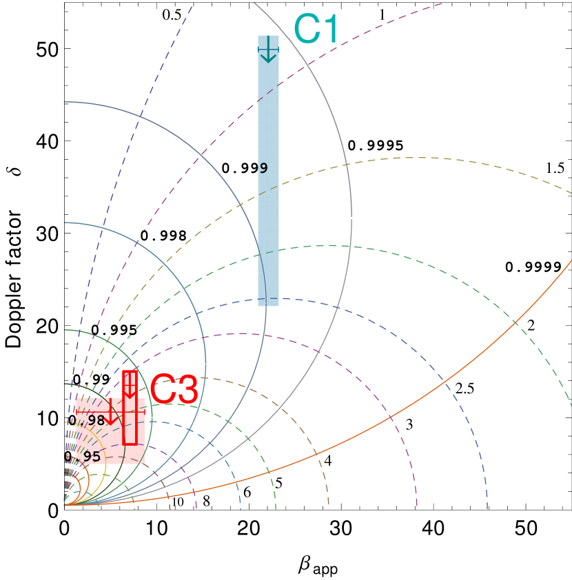
Figure 11: Doppler factor as a function of apparent speed for given viewing angle, $\delta=f(\beta_{\rm app}|\theta)$, and given intrinsic speed $\beta$, $\delta=f(\beta_{\rm app}|\beta)$. Loci represent these two functions for a range of $\theta$ and $\beta$. The values of intrinsic speeds plotted are $\beta=0.9$, $0.95$, $0.98$, $0.99$, $0.995$, $0.998$, $0.999$, $0.9995$, and $0.9999$ shown as solid lines. For the viewing angle the values are $\theta=0.5^{\circ}$, $1^{\circ}$, $1.5^{\circ}$, $2^{\circ}$, $2.5^{\circ}$, $3^{\circ}$, $4^{\circ}$, $5^{\circ}$, $6^{\circ}$, $8^{\circ}$, $10^{\circ}$, $15^{\circ}$, and $30^{\circ}$ shown as dashed lines. Note the two different jet regions, in terms of physical characteristics, where components C1 and C3 are traveling. Shaded areas represent the observables from our VLBI monitoring, namely the Doppler factor and the apparent velocity for each of the two knots.

6 Summary and conclusions

In this paper a comprehensive, three-frequency ($15$, $43$, and $86$ GHz) VLBI study of the $\gamma$-ray blazar PKS $1502{+}106$ was presented, using GMVA and additional data from the MOJAVE monitoring program. Furthermore, we employed the densely-sampled F-GAMMA single-dish light curves at matching frequencies, along with the Fermi/LAT monthly-binned light curve at energies ${>}100$ MeV. The work presented here allows us to follow the multi-frequency flare of $2008$–$2010$ and conclude the following:

1. PKS $1502{+}106$ exhibits a compact, core-dominated morphology at all three frequencies with a one-sided, bent, parsec-scale jet. Component motion within the flow is characterised by high superluminal speeds in the range $5$–$22$ $c$. The most extreme example is component C1 traveling downstream the jet at about $22\,c$ at $15$ GHz and comparable speeds at $43/86$ GHz.

2. Doppler and Lorentz factor estimates for individual components are obtained using variability and VLBI kinematical arguments. The kinematical Doppler and Lorentz factors are $\delta_{\rm C1}\sim\gamma_{\rm min,\,C1}=22.1$ at 15 GHz. For knots C2 and C3, it is $\delta_{\rm C2}\sim\gamma_{\rm min,\,C2}=9.3$ and $\delta_{\rm C3}\sim\gamma_{\rm min,\,C3}=7.2$, respectively. From causality, knot C1, showing significant variability at $15$ GHz, is characterized by $\delta_{\rm var}$ as high as 51.4 and $\gamma_{\rm var}\sim 30.5$. Knot C3 is also found to have consistent behavior at both high frequencies with $\delta_{\rm var}^{\rm 43\,GHz}\sim 12.1$ and $\gamma_{\rm var}^{\rm 43\,GHz}\sim 7.1$, while at 86 GHz the estimation yields $\delta_{\rm var}^{\rm 86\,GHz}\sim 15$ and $\gamma_{\rm var}^{\rm 86\,GHz}\sim 9.2$. All figures are consistent with the estimates of the kinematical Doppler and Lorentz factors. Doppler factors are strikingly different for knot C3 at $r<0.5$ mas and C1 at a distance $r>1$ mas from the core.

3. An additional Doppler factor can be calculated from the different dependencies of $B_{\rm SSA}$ and $B_{\rm eq}$ on $\delta$. The estimate for C1 is in agreement with those from kinematics and causality.

4. Using variability arguments we are able to constrain the viewing angle towards the source to $\theta\sim 3.4^{\circ}$ for the inner and $\theta\sim 0.8^{\circ}$ for the outer portions of the jet, after about $1$ mas. The calculation of the critical viewing angle for knot C1 at $15$ GHz yields $\theta_{\rm c}=2.6^{\circ}$.

5. We calculate the opening angle of the jet of PKS $1502{+}106$ with two methods with the results in very good agreement. The nominal de-projected opening angle is $(3.8\pm 0.5)^{\circ}$.

6. The differences in apparent speed and viewing angle point towards a jet bending after the first mas. This results in differential Doppler boosting – i.e. increasing $\delta$ from ${\sim}12$–$15$ to ${\sim}50$, as traced by components C3 and C1, traveling at radial distances of ${<}0.5$ mas and ${>}1$ mas from the core, respectively. However, this Doppler factor gradient cannot be ascribed to jet bending only. Acceleration must also be at play within the first mas of the jet.

7. By constraining the intrinsic speed, $\beta$, and viewing angle, $\theta$, from the calculated Doppler factors and apparent velocities, we can clearly distinguish between two regions of the jet, wherein knots C1 and C3 are traveling. Specifically, closer to the core at a distance ${\leq}0.5$ mas the parameters obtained for C3 at 43 GHz constrain the parameters of the flow to $0.95\leq\beta\leq 0.995$ and $1.5^{\circ}\leq\theta\leq 10^{\circ}$. The same component at 86 GHz sets slightly stronger constraints to the viewing angle with $3^{\circ}\leq\theta\leq 8^{\circ}$. On the other hand, in the region where C1 is traveling, its observed $\delta$ and $\beta_{\rm app}$ constrain the flow to $\beta\geq 0.999$ and $0.8^{\circ}\leq\theta\leq 2.5^{\circ}$. A clear division is seen between these two jet regions. Hence, we conclude that the jet of PKS $1502{+}106$ bends towards us in the region beyond ${\sim}1$ mas downstream of the core while also accelerating.

8. The radial brightness temperature profile indicates very high $T_{\rm b}$ for the core region at all three frequencies. We find though a trend of decreasing $T_{\rm b}$ as we go towards higher observing frequency and with increasing distance from the core, with no increasing trend. This could indicate a magnetically-dominated core region probed by the $86$ GHz observations where Poynting flux has not yet fully converted to kinetic flux.

9. Component spectra allow the calculation of the magnetic field strength in different regions of the jet. Component C1 exhibits a distinctive SSA peak. The core shows a flat spectrum with $\left<\alpha\right>\sim-0.22$ but at one epoch ($2009.9$) signs of a turnover at ${\sim}43$ GHz. Through the comparison between the SSA and equipartition, minimum magnetic fields we conclude that for component C1, $B_{\rm SSA}$ is much stronger than $B_{\rm eq}$, indicating a high degree of Doppler boosting. Finally, for the core it is $B_{\rm SSA}/\delta\geq 2$ mG and $B_{\rm eq}=1.2$ G.

10. The radio flux density decomposition into distinct VLBI components and comparison with the single-dish radio flux density outburst, indicate that the bulk of radio emission originates from the core at all frequencies. Apart from the core at $43/86$ GHz, knot C3 shares a significant radio flux density level which decays with time. C3 is not resolved at $15$ GHz due to blending with the core.

11. Given the radio flux density decomposition and the estimated ejection time of knot C3 – coincident with the single-dish mm flare onset – we conclude that it is responsible for the radio flare observed in PKS $1502{+}106$ during the period $2008$–$2010$. Furthermore, the previously established correlation between the radio flare and $\gamma$ rays indicates that component C3 is responsible for the $\gamma$-ray flare and its radio counterparts. Arguably, the $2008$–$2010$ flare of PKS $1502{+}106$ is an event originating in a disturbed region at the jet nozzle. While still upstream of the $3$-mm core, it produces the increased $\gamma$-ray emission observed and as it continues to move, it becomes optically thin (at $86$ GHz) close to the $3$-mm VLBI core thus enhancing its brightness. It then continues on and after the 86 GHz optically thick region, is seen as knot C3 at its decaying flux density phase.

12. We conclude that the $\gamma$-ray emitting region is located at ${\leq}5.9$ pc or ${\leq}1.82\times 10^{19}$ cm away from the base of the jet. These estimates constitute upper limits for the distance between the $\gamma$-ray production region and the SMBH itself.

Concluding, PKS $1502{+}106$ represents a source whose complex structural dynamics needs to be further investigated with higher-cadence, high-resolution imaging at mas and sub-mas scales.

Table 11: PKS 1502+106 MODELFIT results at 15 GHz.

Epoch	MJD	Epoch	S	r	PA	FWHM	ID
		ID	(Jy)	(mas)	(∘)	(mas)
2009.23	54915.5	13	$0.038\pm 0.004$	$4.61\pm 0.13$	$103\pm 11$	$4.57\pm 0.46$	…
2002.61	52498.5	1	$0.110\pm 0.011$	$1.98\pm 0.28$	$123\pm 8$	$1.38\pm 0.14$	Ca
2003.24	52727.5	2	$0.103\pm 0.010$	$2.30\pm 0.32$	$123\pm 8$	$1.60\pm 0.16$	Ca
2004.80	53296.5	3	$0.114\pm 0.011$	$2.03\pm 0.36$	$126\pm 10$	$1.79\pm 0.18$	Ca
2005.36	53503.5	4	$0.079\pm 0.008$	$2.65\pm 0.37$	$123\pm 8$	$1.83\pm 0.18$	Ca
2005.73	53636.5	5	$0.102\pm 0.010$	$2.47\pm 0.38$	$122\pm 9$	$1.91\pm 0.19$	Ca
2005.83	53672.5	6	$0.081\pm 0.008$	$2.60\pm 0.31$	$122\pm 7$	$1.55\pm 0.16$	Ca
2005.88	53691.5	7	$0.096\pm 0.010$	$2.27\pm 0.25$	$122\pm 6$	$1.23\pm 0.12$	Ca
2006.52	53923.5	8	$0.093\pm 0.009$	$2.38\pm 0.27$	$123\pm 7$	$1.36\pm 0.14$	Ca
2007.62	54328.5	9	$0.118\pm 0.012$	$2.59\pm 0.33$	$123\pm 7$	$1.66\pm 0.17$	Ca
2008.48	54642.5	10	$0.134\pm 0.013$	$2.46\pm 0.42$	$123\pm 10$	$2.09\pm 0.21$	Ca
2008.60	54684.5	11	$0.100\pm 0.010$	$2.84\pm 0.36$	$123\pm 7$	$1.78\pm 0.18$	Ca
2008.88	54789.5	12	$0.112\pm 0.011$	$2.79\pm 0.42$	$123\pm 9$	$2.11\pm 0.21$	Ca
2009.23	54915.5	13	$0.064\pm 0.006$	$2.93\pm 0.30$	$125\pm 6$	$1.48\pm 0.15$	Ca
2009.94	55175.5	14	$0.088\pm 0.009$	$2.97\pm 0.46$	$122\pm 9$	$2.30\pm 0.23$	Ca
2010.47	55366.5	15	$0.094\pm 0.009$	$3.04\pm 0.53$	$121\pm 10$	$2.67\pm 0.27$	Ca
2010.65	55435.5	16	$0.096\pm 0.010$	$3.00\pm 0.54$	$121\pm 10$	$2.70\pm 0.27$	Ca
2010.87	55513.5	17	$0.098\pm 0.010$	$3.02\pm 0.58$	$121\pm 11$	$2.91\pm 0.29$	Ca
2011.16	55619.5	18	$0.090\pm 0.009$	$3.08\pm 0.58$	$120\pm 11$	$2.89\pm 0.29$	Ca
2011.62	55788.5	19	$0.098\pm 0.010$	$3.22\pm 0.67$	$119\pm 12$	$3.35\pm 0.33$	Ca
2002.61	52498.5	1	$0.165\pm 0.017$	$0.68\pm 0.07$	$120\pm 6$	$0.32\pm 0.03$	Cb
2003.24	52727.5	2	$0.155\pm 0.016$	$0.97\pm 0.11$	$121\pm 6$	$0.54\pm 0.05$	Cb
2004.80	53296.5	3	$0.141\pm 0.014$	$0.84\pm 0.13$	$117\pm 9$	$0.65\pm 0.07$	Cb
2005.36	53503.5	4	$0.127\pm 0.013$	$1.16\pm 0.21$	$122\pm 10$	$1.03\pm 0.10$	Cb
2005.73	53636.5	5	$0.096\pm 0.010$	$1.21\pm 0.19$	$124\pm 9$	$0.96\pm 0.10$	Cb
2005.83	53672.5	6	$0.108\pm 0.011$	$1.19\pm 0.19$	$121\pm 9$	$0.97\pm 0.10$	Cb
2005.88	53691.5	7	$0.045\pm 0.005$	$1.26\pm 0.10$	$136\pm 4$	$0.49\pm 0.05$	Cb
2006.52	53923.5	8	$0.033\pm 0.003$	$1.19\pm 0.14$	$141\pm 7$	$0.10\pm 0.01$	Cb
2003.24	52727.5	2	$0.101\pm 0.010$	$0.37\pm 0.13$	$123\pm 19$	$0.10\pm 0.01$	Cc
2004.80	53296.5	3	$0.129\pm 0.013$	$0.42\pm 0.13$	$98\pm 17$	$0.10\pm 0.01$	Cc
2005.36	53503.5	4	$0.157\pm 0.016$	$0.58\pm 0.10$	$101\pm 10$	$0.50\pm 0.05$	Cc
2005.73	53636.5	5	$0.119\pm 0.012$	$0.64\pm 0.10$	$100\pm 9$	$0.52\pm 0.05$	Cc
2005.83	53672.5	6	$0.087\pm 0.009$	$0.66\pm 0.10$	$99\pm 8$	$0.48\pm 0.05$	Cc
2005.88	53691.5	7	$0.110\pm 0.011$	$0.71\pm 0.12$	$97\pm 9$	$0.57\pm 0.06$	Cc
2006.52	53923.5	8	$0.061\pm 0.006$	$0.82\pm 0.15$	$90\pm 10$	$0.75\pm 0.07$	Cc
2008.48	54642.5	10	$0.037\pm 0.004$	$1.30\pm 0.13$	$99\pm 6$	$0.10\pm 0.01$	Cc
2008.60	54684.5	11	$0.101\pm 0.010$	$1.14\pm 0.14$	$103\pm 7$	$0.72\pm 0.07$	Cc
2008.88	54789.5	12	$0.036\pm 0.004$	$1.47\pm 0.08$	$103\pm 3$	$0.39\pm 0.04$	Cc
2009.23	54915.5	13	$0.056\pm 0.006$	$1.35\pm 0.20$	$105\pm 8$	$0.98\pm 0.10$	Cc
2007.62	54328.5	9	$0.278\pm 0.028$	$0.61\pm 0.08$	$97\pm 7$	$0.38\pm 0.04$	C1
2008.48	54642.5	10	$0.118\pm 0.012$	$0.77\pm 0.05$	$94\pm 3$	$0.23\pm 0.02$	C1
2008.60	54684.5	11	$0.072\pm 0.007$	$0.76\pm 0.14$	$91\pm 11$	$0.10\pm 0.01$	C1
2008.88	54789.5	12	$0.147\pm 0.015$	$0.80\pm 0.06$	$95\pm 5$	$0.32\pm 0.03$	C1
2009.23	54915.5	13	$0.054\pm 0.005$	$0.92\pm 0.15$	$92\pm 9$	$0.10\pm 0.01$	C1
2009.94	55175.5	14	$0.037\pm 0.004$	$1.26\pm 0.18$	$98\pm 8$	$0.89\pm 0.09$	C1
2010.47	55366.5	15	$0.037\pm 0.004$	$1.30\pm 0.15$	$97\pm 7$	$0.77\pm 0.08$	C1
2010.65	55435.5	16	$0.027\pm 0.003$	$1.38\pm 0.13$	$93\pm 5$	$0.64\pm 0.06$	C1
2010.87	55513.5	17	$0.026\pm 0.003$	$1.47\pm 0.13$	$96\pm 5$	$0.66\pm 0.07$	C1
2011.16	55619.5	18	$0.020\pm 0.002$	$1.57\pm 0.09$	$98\pm 3$	$0.43\pm 0.04$	C1
2011.62	55788.5	19	$0.027\pm 0.003$	$1.58\pm 0.12$	$105\pm 4$	$0.59\pm 0.06$	C1
2008.48	54642.5	10	$0.105\pm 0.011$	$0.32\pm 0.13$	$90\pm 23$	$0.10\pm 0.01$	C2
2008.60	54684.5	11	$0.117\pm 0.012$	$0.35\pm 0.14$	$98\pm 22$	$0.10\pm 0.01$	C2
2008.88	54789.5	12	$0.100\pm 0.010$	$0.43\pm 0.14$	$101\pm 19$	$0.10\pm 0.01$	C2
2009.23	54915.5	13	$0.137\pm 0.014$	$0.58\pm 0.06$	$99\pm 6$	$0.32\pm 0.03$	C2
2009.94	55175.5	14	$0.141\pm 0.014$	$0.74\pm 0.09$	$100\pm 7$	$0.44\pm 0.04$	C2
2010.47	55366.5	15	$0.123\pm 0.012$	$0.71\pm 0.11$	$103\pm 9$	$0.54\pm 0.05$	C2
2010.65	55435.5	16	$0.120\pm 0.012$	$0.74\pm 0.11$	$103\pm 9$	$0.57\pm 0.06$	C2
2010.87	55513.5	17	$0.112\pm 0.011$	$0.77\pm 0.11$	$105\pm 8$	$0.56\pm 0.06$	C2
2011.16	55619.5	18	$0.118\pm 0.012$	$0.81\pm 0.11$	$108\pm 8$	$0.56\pm 0.06$	C2
2011.62	55788.5	19	$0.098\pm 0.010$	$0.82\pm 0.14$	$113\pm 10$	$0.69\pm 0.07$	C2
2002.61	52498.5	1	$1.341\pm 0.134$	$0.00\pm 0.02$	$0.0\pm 0.0$	$0.23\pm 0.02$	Core
2003.24	52727.5	2	$1.457\pm 0.146$	$0.00\pm 0.02$	$0.0\pm 0.0$	$0.22\pm 0.02$	Core
2004.80	53296.5	3	$0.611\pm 0.061$	$0.00\pm 0.02$	$0.0\pm 0.0$	$0.20\pm 0.02$	Core
2005.36	53503.5	4	$0.505\pm 0.051$	$0.00\pm 0.12$	$0.0\pm 0.0$	$0.11\pm 0.01$	Core
2005.73	53636.5	5	$0.803\pm 0.080$	$0.00\pm 0.01$	$0.0\pm 0.0$	$0.12\pm 0.01$	Core
2005.83	53672.5	6	$0.868\pm 0.087$	$0.00\pm 0.12$	$0.0\pm 0.0$	$0.11\pm 0.01$	Core
2005.88	53691.5	7	$0.926\pm 0.093$	$0.00\pm 0.15$	$0.0\pm 0.0$	$0.11\pm 0.01$	Core
2006.52	53923.5	8	$1.339\pm 0.134$	$0.00\pm 0.02$	$0.0\pm 0.0$	$0.23\pm 0.02$	Core
2007.62	54328.5	9	$1.113\pm 0.111$	$0.00\pm 0.12$	$0.0\pm 0.0$	$0.09\pm 0.01$	Core
2008.48	54642.5	10	$1.348\pm 0.135$	$0.00\pm 0.12$	$0.0\pm 0.0$	$0.09\pm 0.01$	Core
2008.60	54684.5	11	$1.320\pm 0.132$	$0.00\pm 0.12$	$0.0\pm 0.0$	$0.08\pm 0.01$	Core
2008.88	54789.5	12	$1.589\pm 0.159$	$0.00\pm 0.12$	$0.0\pm 0.0$	$0.08\pm 0.01$	Core
2009.23	54915.5	13	$2.815\pm 0.282$	$0.00\pm 0.13$	$0.0\pm 0.0$	$0.06\pm 0.01$	Core
2009.94	55175.5	14	$1.213\pm 0.121$	$0.00\pm 0.12$	$0.0\pm 0.0$	$0.09\pm 0.01$	Core
2010.47	55366.5	15	$0.723\pm 0.072$	$0.00\pm 0.13$	$0.0\pm 0.0$	$0.10\pm 0.01$	Core
2010.65	55435.5	16	$0.749\pm 0.075$	$0.00\pm 0.12$	$0.0\pm 0.0$	$0.09\pm 0.01$	Core
2010.87	55513.5	17	$0.880\pm 0.088$	$0.00\pm 0.12$	$0.0\pm 0.0$	$0.09\pm 0.01$	Core
2011.16	55619.5	18	$1.003\pm 0.100$	$0.00\pm 0.12$	$0.0\pm 0.0$	$0.09\pm 0.01$	Core
2011.62	55788.5	19	$1.127\pm 0.113$	$0.00\pm 0.13$	$0.0\pm 0.0$	$0.09\pm 0.01$	Core

Table 11: continued.

Table 12: PKS 1502+106 MODELFIT results at 43 GHz.

Epoch	MJD	Epoch	S	r	PA	FWHM	ID
		ID	(Jy)	(mas)	(∘)	(mas)
2009.35	54959.36	1	$0.055\pm 0.006$	$0.93\pm 0.08$	$94\pm 5$	$0.404\pm 0.040$	C1
2009.78	55117.82	2	$0.109\pm 0.011$	$0.87\pm 0.08$	$99\pm 5$	$0.404\pm 0.040$	C1
2010.34	55323.28	3	$0.044\pm 0.004$	$1.08\pm 0.19$	$97\pm 10$	$0.965\pm 0.096$	C1
2011.35	55688.76	4	$0.056\pm 0.006$	$1.20\pm 0.24$	$107\pm 11$	$1.211\pm 0.121$	C1
2011.77	55843.86	5	$0.043\pm 0.004$	$1.20\pm 0.20$	$103\pm 10$	$1.017\pm 0.102$	C1
2012.38	56065.17	6	$0.041\pm 0.004$	$1.35\pm 0.29$	$97\pm 12$	$1.467\pm 0.147$	C1
2009.35	54959.36	1	$0.059\pm 0.006$	$0.57\pm 0.04$	$100\pm 4$	$0.202\pm 0.020$	C2
2009.78	55117.82	2	$0.044\pm 0.004$	$0.49\pm 0.07$	$99\pm 8$	$0.040\pm 0.004$	C2
2010.34	55323.28	3	$0.031\pm 0.003$	$0.74\pm 0.03$	$100\pm 3$	$0.160\pm 0.016$	C2
2011.35	55688.76	4	$0.025\pm 0.003$	$0.78\pm 0.04$	$108\pm 3$	$0.191\pm 0.019$	C2
2011.77	55843.86	5	$0.014\pm 0.001$	$0.71\pm 0.03$	$108\pm 2$	$0.130\pm 0.013$	C2
2012.38	56065.17	6	$0.011\pm 0.001$	$0.65\pm 0.03$	$120\pm 3$	$0.159\pm 0.016$	C2
2009.35	54959.36	1	$0.554\pm 0.055$	$0.08\pm 0.06$	$130\pm 37$	$0.030\pm 0.003$	C3
2009.78	55117.82	2	$0.108\pm 0.011$	$0.14\pm 0.07$	$126\pm 26$	$0.040\pm 0.004$	C3
2010.34	55323.28	3	$0.042\pm 0.004$	$0.22\pm 0.04$	$115\pm 10$	$0.194\pm 0.019$	C3
2011.35	55688.76	4	$0.032\pm 0.003$	$0.18\pm 0.08$	$61\pm 23$	$0.040\pm 0.004$	C3
2011.77	55843.86	5	$0.080\pm 0.008$	$0.14\pm 0.02$	$70\pm 7$	$0.089\pm 0.009$	…
2012.38	56065.17	6	$0.068\pm 0.007$	$0.13\pm 0.07$	$70\pm 28$	$0.050\pm 0.005$	…
2009.35	54959.36	1	$3.030\pm 0.303$	$0.00\pm 0.06$	$0.0\pm 0.0$	$0.029\pm 0.003$	Core
2009.78	55117.82	2	$2.301\pm 0.230$	$0.00\pm 0.07$	$0.0\pm 0.0$	$0.056\pm 0.006$	Core
2010.34	55323.28	3	$0.530\pm 0.053$	$0.00\pm 0.07$	$0.0\pm 0.0$	$0.054\pm 0.005$	Core
2011.35	55688.76	4	$1.067\pm 0.107$	$0.00\pm 0.03$	$0.0\pm 0.0$	$0.131\pm 0.013$	Core
2011.77	55843.86	5	$0.993\pm 0.099$	$0.00\pm 0.01$	$0.0\pm 0.0$	$0.073\pm 0.007$	Core
2012.38	56065.17	6	$0.799\pm 0.080$	$0.00\pm 0.07$	$0.0\pm 0.0$	$0.040\pm 0.004$	Core

Table 12: continued.

Table 13: PKS 1502+106 MODELFIT results at 86 GHz.

Epoch	MJD	Epoch	S	r	PA	FWHM	ID
		ID	(Jy)	(mas)	(∘)	(mas)
2009.35	54959.36	1	$0.071\pm 0.007$	$1.18\pm 0.16$	$99\pm\dots$	$0.780\pm 0.078$	…
2010.34	55323.28	3	$0.011\pm 0.001$	$1.39\pm 0.08$	$100\pm\dots$	$0.135\pm 0.014$	…
2012.38	56065.54	6	$0.004\pm 0.001$	$1.78\pm 0.06$	$100\pm\dots$	$0.100\pm 0.010$	…
2009.78	55117.82	2	$0.031\pm 0.003$	$0.86\pm 0.05$	$103\pm 1$	$0.065\pm 0.006$	C1
2010.34	55323.28	3	$0.008\pm 0.001$	$0.97\pm 0.08$	$93\pm 5$	$0.018\pm 0.002$	C1
2012.38	56065.54	6	$0.010\pm 0.001$	$1.50\pm 0.06$	$107\pm 1$	$0.052\pm 0.005$	C1
2009.35	54959.36	1	$0.010\pm 0.001$	$0.49\pm 0.06$	$102\pm 7$	$0.016\pm 0.002$	C2
2009.78	55117.82	2	$0.033\pm 0.003$	$0.46\pm 0.05$	$106\pm 2$	$0.061\pm 0.006$	C2
2010.34	55323.28	3	$0.018\pm 0.002$	$0.62\pm 0.05$	$117\pm 5$	$0.269\pm 0.027$	C2
2011.35	55688.76	4	$0.013\pm 0.001$	$0.63\pm 0.07$	$84\pm 6$	$0.331\pm 0.033$	C2
2011.77	55843.86	5	$0.024\pm 0.002$	$0.79\pm 0.04$	$110\pm 3$	$0.211\pm 0.021$	C2
2012.38	56065.54	6	$0.011\pm 0.001$	$0.75\pm 0.04$	$124\pm 3$	$0.197\pm 0.020$	C2
2009.35	54959.36	1	$0.446\pm 0.045$	$0.07\pm 0.06$	$137\pm 43$	$0.016\pm 0.002$	C3
2009.78	55117.82	2	$0.056\pm 0.006$	$0.15\pm 0.05$	$110\pm 19$	$0.016\pm 0.002$	C3
2010.34	55323.28	3	$0.014\pm 0.001$	$0.20\pm 0.08$	$132\pm 22$	$0.024\pm 0.002$	C3
2011.35	55688.76	4	$0.023\pm 0.002$	$0.27\pm 0.07$	$101\pm 15$	$0.016\pm 0.002$	C3
2012.38	56065.54	6	$0.009\pm 0.001$	$0.36\pm 0.06$	$142\pm 10$	$0.015\pm 0.002$	C3
2009.35	54959.36	1	$0.032\pm 0.003$	$0.25\pm 0.06$	$134\pm 14$	$0.016\pm 0.002$	…
2009.78	55117.82	2	$0.016\pm 0.002$	$0.27\pm 0.05$	$99\pm 11$	$0.016\pm 0.002$	…
2011.35	55688.76	4	$0.032\pm 0.003$	$0.06\pm 0.07$	$30\pm 5$	$0.029\pm 0.003$	…
2011.77	55843.86	5	$0.024\pm 0.002$	$0.17\pm 0.06$	$103\pm 19$	$0.022\pm 0.002$	…
2009.35	54959.36	1	$2.293\pm 0.229$	$0.00\pm 0.06$	$0.0\pm 0.0$	$0.031\pm 0.003$	Core
2009.78	55117.82	2	$0.966\pm 0.097$	$0.00\pm 0.05$	$0.0\pm 0.0$	$0.029\pm 0.003$	Core
2010.34	55323.28	3	$0.564\pm 0.056$	$0.00\pm 0.08$	$0.0\pm 0.0$	$0.038\pm 0.004$	Core
2011.35	55688.76	4	$0.808\pm 0.081$	$0.00\pm 0.07$	$0.0\pm 0.0$	$0.026\pm 0.003$	Core
2011.77	55843.86	5	$0.612\pm 0.061$	$0.00\pm 0.06$	$0.0\pm 0.0$	$0.036\pm 0.004$	Core
2012.38	56065.54	6	$0.583\pm 0.058$	$0.00\pm 0.06$	$0.0\pm 0.0$	$0.027\pm 0.003$	Core

Table 13: continued.

Appendix A VLBI component light curves

The appendix plots feature all VLBI component light curves at all observing frequencies (Fig. 12).

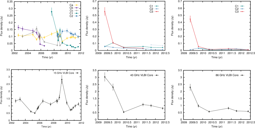
Figure 12: Light curves of individual components (top panels) and the core (bottom panels) at $15$, 43 GHz, and 86 GHz. Component C1 shows significant variability between $2008$ and $2010$ (at $15$ GHz). Also note component C3 at its decaying flux density phase, seen only at high-frequency observations.