Characterization of Kepler-91b and the Investigation of a Potential Trojan Companion Using EXONEST
Abstract
Presented here is an independent re-analysis of the Kepler light curve of Kepler-91 (KIC 8219268). Using the EXONEST software package, which provides both Bayesian parameter estimation and Bayesian model testing, we were able to re-confirm the planetary nature of Kepler-91b. In addition to the primary and secondary eclipses of Kepler-91b, a third dimming event appears to occur approximately away (in phase) from the secondary eclipse, leading to the hypothesis that a Trojan planet may be located at the L4 or L5 Lagrange points. Here, we present a comprehensive investigation of four possibilities to explain the observed dimming event using all available photometric data from the Kepler Space Telescope, recently obtained radial velocity measurements, and N-body simulations. We find that the photometric model describing Kepler-91b and a Trojan planet is highly favored over the model involving Kepler-91b alone. However, it predicts an unphysically high temperature for the Trojan companion, leading to the conclusion that the extra dimming event is likely a false-postive.
1 Introduction
| Stellar Parameters From Literature | |
|---|---|
| Mass, | |
| Radius, | |
| Effective Temperature, (K) | |
| Surface Gravity, | |
| Gravity Darkening Exponent | |
| Lin. Limb Darkening Coeff. | |
| Quad. Limb Darkening Coeff. () | |
| Kepler Magnitude | 12.495 |
| Estimated Planetary Parameters | |
| Mass, | |
| Radius, | |
| Density, | |
| Period, | |
| Inclination, | |
| Eccentricity | |
| Equilibrium Temperature, (K) |
Kepler-91 (KIC 8219268) is a red giant branch star in a late stage of stellar evolution. It is orbited by at least one companion (Kepler-91b), which was determined to be of planetary nature by Lillo-Box et al. (2013). The planetary status has been refuted by two independent groups (Esteves, De Mooij, and Jayawardhana, 2013; Sliski and Kipping, 2014), but has since been confirmed by radial velocity measurements (Barclay et al., 2014; Lillo-Box et al., 2014). Kepler-91b previously has been estimated to be a transiting Jupiter-mass planet () that orbits its red giant host star at one of the shortest known orbital distances of just with an orbital period of days (Batalha et al., 2013; Lillo-Box et al., 2013, 2014) (Literature values in Table 1). It orbits its host star in a slightly eccentric orbit of inclined by with respect to the plane of the sky. Being so close to such a giant star (), even at this low inclination the planet is still observed to transit Kepler-91. In addition to the primary transit and secondary eclipse corresponding to Kepler-91b, Lillo-Box et al. (2013) observed what appears to be a third occultation that occurs approximately in orbital phase away from the secondary eclipse. They describe four potential hypotheses explaining this dimming event: (1) a transiting Trojan planet located at either the L4 or L5 Lagrange point, (2) a second more distant planet in a resonant, non-coplanar orbit, (3) the presence of a large transiting exomoon in a resonant orbit around Kepler-91b, (4) instrumental effects associated with the Kepler pipeline or stellar variability.
Previous theoretical studies of exo-Trojans include numerical simulations to investigate the stability of such worlds (Dvorak et al., 2004; Schwarz et al., 2007, 2009), as well as the effect that a Trojan planet would have on the observed transit times of the primary planet (Transit Timing Variations) (Ford and Gaudi, 2006; Ford and Holman, 2007; Madhusudhan and Winn, 2009), and a search for Trojans in binary systems based on anomalies in the light curves associated with the correct phase expected from a Trojan (Caton et al., 2001). Despite these studies, the definitive discovery of such a planet remains elusive.
Presented here is a brief discussion of the four possible hypotheses intended to describe the observed flux, and an analysis of approximately days worth of Kepler observations and published radial velocity measurements of the Kepler-91 system. Three planetary models are applied to the Kepler-91 light curve: two, which model the photometric and radial velocity signals from a single planet, Kepler-91b, in the case of both circular and eccentric orbits, and another that models the photometric and radial velocity signals from Kepler-91b and an exo-Trojan in an eccentric orbit. The analysis was performed using the EXONEST software package (Placek et al., 2014), which relies on Bayesian model selection to statistically test between competing models, thus determining which model best describes a given dataset. Since at present, there are no confirmed instances of exo-Trojans, this would be the first photometric evidence of an entirely new class of exoplanet. Furthermore, its existence would provide a unique opportunity to study the effect of stellar flux on two different planets in identical orbits.
1.1 The Trojan Hypothesis
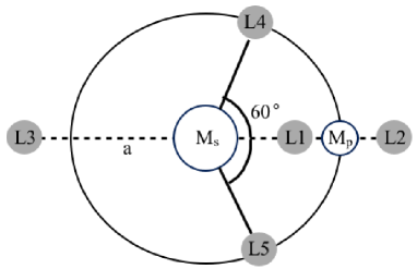
In the restricted three-body problem, there are five equilibrium points known as Lagrange points. The points L1, L2, and L3 lie on the line connecting the primary planet to the host star, whereas L4 and L5 are positioned in front of, or behind, the primary planet in its own orbit as shown in Figure 1. Any object located at the L4 or L5 Lagrange point will appear stationary (neglecting librations) in a co-rotating reference frame. That is, it will orbit the host star with the same period as that of the primary planet. These orbits at L4 and L5 are stable provided that the host star is greater than 24.96 times the mass of the primary planet, whereas L1, L2, and L3 are unstable saddle points of the gravitational effective potential.
A massive object located at the L4 or L5 Lagrange point will undergo librational motion. The object will display long-period librations about the Lagrange point with period
| (1) |
where is the orbital period of the primary planet, and , as well as epicyclic librations with period
| (2) |
The phase difference of between the secondary eclipse of Kepler-91b and the third dimming event observed in the Kepler-91 light curve makes the possibility of a Trojan body very enticing. However, it should be noted that this dimming event would have to be the result of the secondary eclipse of the Trojan — not the primary transit. If it were a primary transit, then the second body would be out of phase from Kepler-91b by , and thus not be a Trojan. The fact that this signal appears in the light curve folded at the orbital period of Kepler-91b, implies that it either occurs at the same period as Kepler-91b, or at an integer value of that period.
1.2 The Distant Planet Hypothesis
As mentioned in the previous section, this signal could be the transit of a more distant planet in a non-coplanar, resonant orbit to that of Kepler-91b. The low signal to noise of the raw Kepler light curve of Kepler-91 makes it difficult to simulate such a complex situation, however by considering the light curve folded on the period of Kepler-91b, one may be able to determine the likelihood of such a configuration. If the occultation is due to the presence of a more distant resonant planet, one would expect differences between the occultations occurring at odd, or even integrals of the orbital period of Kepler-91b.
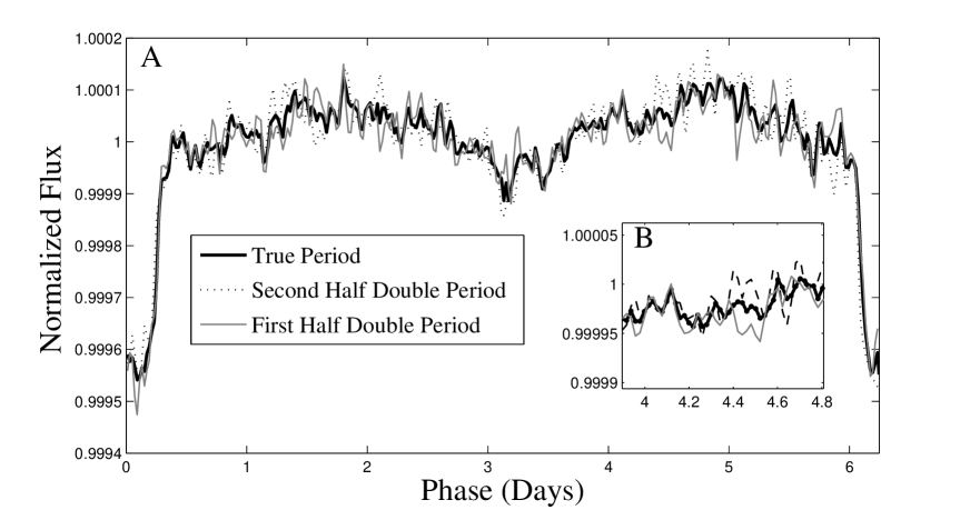
Figure 2, shows the binned time series for Kepler-91b, folded at the accepted orbital period of Kepler-91b (solid black curve), and twice that of Kepler-91b (solid gray and dashed black curves). One can clearly see differences between the third dimming event occurring during the first and second halves of the double-period. While there appears to still be an occultation occurring, there is an odd feature toward one side of the dimming. During the first half of the double-period, there is an increase in the flux while during the second half of the double-period there is a decrease occurring at the same orbital phase, which can be seen more clearly in Figure 2B. There are however significant odd/even effects for the primary eclipse of Kepler-91b as well, implying that this hypothesis may not be the correct explanation. These odd/even effects will be discussed in more detail in Section 3.5
1.3 The Exomoon Hypothesis
A sizable exomoon in a resonant orbit may also be the cause of this third dimming event. The moon would need to appear to transit Kepler-91b in phase before or after its secondary eclipse of the host star. In addition, this exomoon would need to have an orbital period that is the same as, or an integer multiple of that associated with Kepler-91b. This exomoon hypothesis and the stability of such a configuration is discussed in detail in Section 3.4.
1.4 Instrumental Effects and Stellar Variability
The Kepler science pipeline component Presearch Data Conditioning (PDC) identifies and removes systematic errors that are highly correlated across the ensemble of target stars on each CCD readout channel. It also identifies outliers and transients associated with radiation damage to the CCDs at the pixel level, called sudden pixel sensitivity dropouts. Global instrumental signatures are identified via singular value decomposition (SVD) of the quiet stars on each CCD readout channel. PDC-MAP applies a Bayesian maximum a posteriori (MAP) approach (Stumpe et al., 2014; Smith et al., 2012) to constrain the fit coefficients for the SVD-identified co-trending basis vectors that are then projected out of each stellar light curve. This data reduction step can coincidentally remove stellar variations correlated with the instrumental signatures, especially on timescales longer than 20 days and can in some cases, introduce systematic signatures into individual light curves. However, it is highly unlikely that PDC-MAP introduced consistent brightening and dimming events at the period of Kepler-91b, as such signatures are not evident in the co-trending basis vectors which are formulated for each individual observing segment or quarter. Moreover, the transits and secondary occultation of Kepler-91b and the deep secondary occultation of the candidate Trojan planet are readily identifiable in the simple aperture photometry (PA-SAP) produced by the Kepler science pipeline, in addition to the PDC-MAP light curves analyzed in this paper (Jenkins et al., 2010; Twicken et al., 2010).
Lillo-Box et al. (2013) were able to exclude stellar oscillations as the source of the extra dimming by performing a zero-order cleaning of the solar-like oscillations of the star using a high-pass filter in Fourier space.
2 Methods
For this analysis, we utilized the EXONEST software package (Knuth, Placek, and Richards, 2012; Placek, Richards, and Knuth, 2013, 2014), which employs a Bayesian inference engine capable of employing Nested Sampling (Skilling et al., 2006) and MultiNest (Feroz, Hobson, and Bridges, 2009, 2011, 2013), as well as Metropolis-Hastings Markov chain Monte Carlo (MCMC) (Metropolis et al., 1953) and Simulated Annealing (Otten and van Ginneken, 1989). The Multi-Nest engine was employed for this study for its ability to efficiently explore complicated parameter spaces.
The EXONEST software package provides the ability to perform both Bayesian parameter estimation and model testing. That is, given a photometric model that describes a hypothetical planetary system, EXONEST allows one to obtain model parameter estimates as well as an estimate of the Bayesian evidence, which is used to statistically test one model against another. A model found to have an overwhelmingly large corresponding evidence value compared to the others is then said to be favored over the other model(s) describing the particular dataset (Sivia and Skilling, 2006; Knuth et al., 2015). The measure of one model’s favorability over another is quantified by the Bayes’ factor, which is the ratio of the model evidences. Nested Sampling and Multi-Nest both compute log-evidences, so the Bayes’ factor is calculated as the exponential of the difference between the log-evidences.
EXONEST currently models four physical mechanisms in addition to transits and secondary eclipses that affect the photometric signal obtained from an exoplanetary system. The first is the reflection of starlight off of the atmosphere or surface of the planet (Seager et al., 2000; Jenkins and Doyle, 2003; Seager, 2010; Perryman, 2011; Placek et al., 2014), which is given by
| (3) |
where is the geometric albedo, is the planetary radius, is the star-planet separation distance, and is the planetary phase angle. The second is the thermally-emitted light from both the day- and night-sides of the planet (Charbonneau et al., 2005; Borucki et al., 2009; Placek et al., 2014), given by
| (4) |
and
| (5) |
where , and are the day- and night-side temperatures of the planet, is the radius of the host star, and is the observed thermal radiation in the Kepler bandpass from a blackbody emitter at temperature . Both of these effects induce variations in the observed light as the planet orbits its host star and it goes through its phases (New, Crescent, Quarter, Full). The third effect is Doppler beaming (or Boosting), which is a relativistic effect that causes an increase in observed flux when the host star is moving toward an observer, and a decrease when the star recedes from the observer (Rybicki and Lightman, 2008; Loeb and Gaudi, 2003; Placek et al., 2014). This induces variations in the observed light curve since stars with planets around them orbit the common center of mass of the system, and thus periodically move toward and away from an observer. The relative flux due to Doppler beaming is found by
| (6) |
where is the stellar radial velocity along the observer’s line of sight. The fourth effect accounts for ellipsoidal variation, which are due to the gravitational tidal warping of the stellar surface due to the proximity of a massive planet (Loeb and Gaudi, 2003; Placek et al., 2014; Faigler and Mazeh, 2011; Esteves et al., 2013; Shporer et al., 2011). A massive planet will warp the stellar surface into an ellipsoid whose semi-axis will follow the planet throughout its orbit. This results in observed flux variations at the orbital period (twice the frequency) due to both the changing cross-sectional area of the star and an accompanying gravity darkening at the sub-planetary point and at the corresponding antipodal point. This is approximated as
| (7) |
where and are the planetary and stellar masses, is the orbital inclination, and is related to the linear limb-darkening coefficient , and the gravity darkening coefficient by
| (8) |
In addition to modeling the photometric effects in the case of both circular and eccentric orbits for Kepler-91b alone, a two-planet model was created, which assumed that the orbit of a second body is of the same orbital period (), eccentricity (), inclination (), and argument of periastron () as that of Kepler-91b, but offset by an orbital phase of .
Kepler data from quarters 1-16 were used to analyze Kepler-91, which spans approximately days, and includes 63,214 data points. The following stellar properties were also assumed: , , , (Claret and Bloemen, 2011; Esteves et al., 2013). Here, the parameters and represent the linear limb-darkening coefficient and gravity-darkening coefficient respectively. Similarly, the parameters and represent the quadratic limb-darkening coefficients. The data were also folded on the accepted value of the orbital period, which assumes that both objects have an orbital period of days.
2.1 Prior Probabilities and
The Likelihood Function
The Bayesian inference engine takes as inputs the prior probabilities for each model parameter and a likelihood function describing the expected noise distribution.
The prior probability distribution of a particular model parameter quantifies the knowledge one has about that parameter before analyzing the data. For this study, each model parameter is assigned an uninformative uniform prior probability over a reasonable range as shown in Table 2. Since stellar characteristics such as mass, radius, and effective temperature have all been estimated previously, we assign a Gaussian prior (Table 2) for these parameters defined by the published values in Table 1.
| Parameter | Distribution |
|---|---|
| Dayside Temp., (K) | |
| Nightside Temp., (K) | |
| Orbital Inclination, | |
| Orbital Eccentricity, | |
| Argument of Periastron, | |
| Initial Mean Anomaly, | |
| Stellar Mass, | |
| Stellar Radius, | |
| Planetary Radius, | |
| Planetary Mass, | |
| Geometric Albedo, | |
| Standard Dev. of noise, (ppm) | |
| Correlation Strength, | |
| Fixed Values | |
| Orbital Period, (d) | |
| Quad. Limb Darkening | |
| Linear Limb Darkening | |
| Gravity Darkening | |
The likelihood function depends on the particular forward model and the expected nature of the noise. In many situations one may assume that the noise is Gaussian distributed, however Kepler-91 displays a significant amount of correlated (red) noise likely induced by stellar oscillations. In order to accomodate the presence of correlated noise, we employ a nearest-neighbor approach introduced by Sivia and Skilling (2006) where the strength of correlations among nearest neighbors is described by the parameter , which varies from . Taking these nearest neighbor correlations into account one can obtain a log-likelihood function of the form (Sivia and Skilling, 2006)
| (9) |
where is the number of data points, the noise variance, and is related to the sum of the squared residuals, , by
| (10) |
Here, is defined as the sum of the first and last squared residuals, and is the sum of the nearest neighbor residuals, which can be calculated using
| (11) |
Note that when the correlation strength, , the log-likelihood function reduces to a Gaussian distribution of the form
| (12) |
For this study, both the correlated noise likelihood (9) and a Gaussian likelihood (12) are used to analyze the Kepler-91b timeseries.
3 Results
This section summarizes our results from modeling the Kepler photometry from quarters 1-16 and the published radial velocity measurements of Kepler-91b (Lillo-Box et al., 2014; Barclay et al., 2014). In addition, a short study of the stability of the hypothesized Trojan is presented using parameter values predicted by our analysis of the Kepler data.
3.1 From Photometry
Results from our analyses are summarized in Table 3. The parameter estimates obtained from the one-planet model (Kepler-91b only) indicate that Kepler-91b is a hot-Jupiter with a mass of and radius of consistent with results from Lillo-Box et al. (2013). The dayside temperature was found to be . However, this may be significantly underestimated due to the mid-eclipse brightening event, which can be seen in Figure 6 at orbital phase of . This day-side temperature is consistent with the equilibrium temperature calculated by Lillo-Box et al. (2013) assuming all incident thermal flux is re-radiated back into space (). Based on the model log-evidences, the eccentric orbit model is significantly favored over the circular orbit model by a Bayes’ factor of . However, the derived orbital eccentricity was lower than that of Lillo-Box et al. (2013) at .
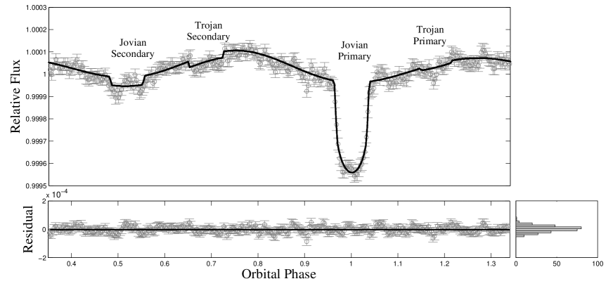
In the case of the two-planet model, which considers a photometric signal from both Kepler-91b and the hypothesized Trojan, the log-evidence was such that the two-planet eccentric orbit model is favored by a Bayes’ factor of million over the single planet eccentric orbit model. The improvement in fitting is also demonstrated by the increased maximum likelihood of the solution and lower (see Table 3). The predicted composite photometric signal from both objects is displayed in Figure 6. Note that the third occultation that occurs around orbital phase is modeled by EXONEST as the secondary eclipse of the Trojan, as predicted, as well as a fourth occultation around an orbital phase of , which represents the transit of the Trojan. Parameter estimates associated with Kepler-91b do not change significantly by adding another planet to the model. The mass , radius , albedo , and dayside temperature are all within of the estimates from the one-planet model. Parameter estimates from the two-planet eccentric model suggest that the hypothesized Trojan has a mass of or , and radius of giving it a mean density of , which implies that, if this is a planet, it could potentially be classified as sub-Neptunian. This estimate of the density is consistent with results from Rogers (2014), who showed using the known populations of sub-Neptune planets that planets with radii greater than are most likely not rocky, but gaseous. In addition, the presence of a Trojan body is not only supported by the log-evidence calculations, but also by the model prediction for the planet-Trojan phase difference, which is degrees.
This model also predicted very high day and night-side brightness temperatures of K and K, respectively, which will be further discussed in Section 4. As for the primary planet, the two-planet model predicts Kepler-91b to have day and night-side temperatures that are within of each other ( and ), which is not unexpected for short-period hot Jupiters around red giant stars (Spiegel and Madhusudhan, 2012).
This model also predicted an unexpectedly high albedo for the Trojan , which is likely due to the strong degeneracy between the albedo and the day-side temperature . As indicated by the large uncertainties, there is simply not enough information in the data for EXONEST to disentangle the reflected and emitted components and to well-determine the geometric albedo of the hypothetical Trojan.
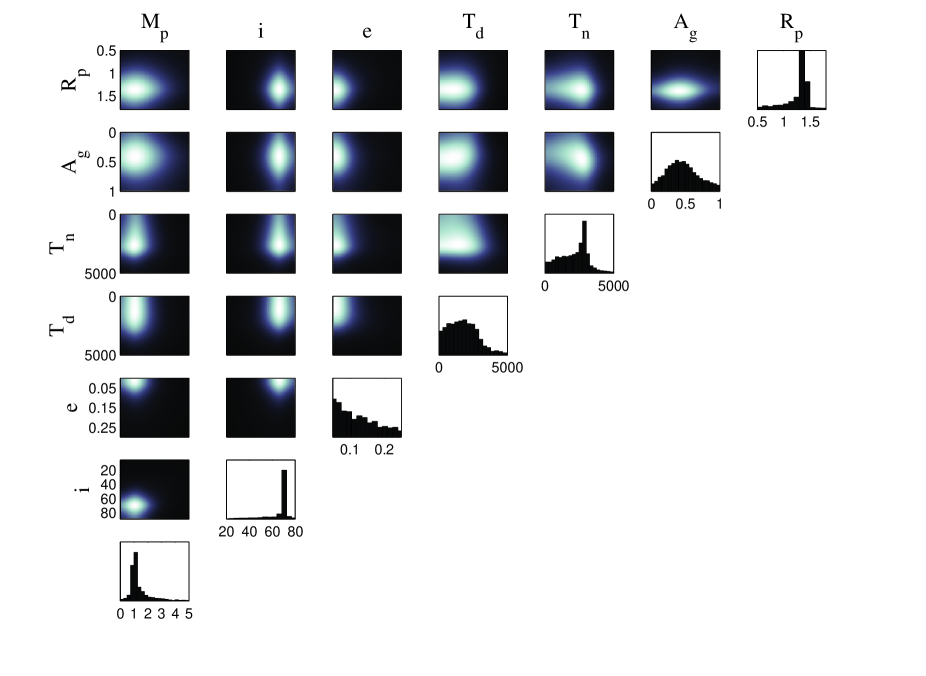
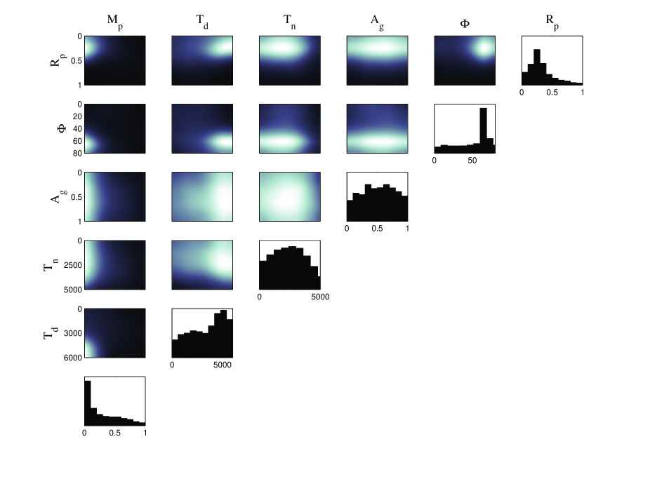
Two-dimensional representations of the posterior probability of the model parameters are illustrated in Figures 4 and 5. Notice the degeneracy between and in Figure 4. A planet can have a higher day-side temperature and lower geometric albedo and output the same flux as a highly reflective planet (high geometric albedo) with a low day-side temperature. One can also see that many of the parameters associated with the Trojan exhibit broad ridge-like structures, which explain our inability to precisely estimate them.
Based on the estimate of the Jovian mass obtained from the two-planet model, the expected long- and short-period librations of the Trojan can be calculated to be days, and days, respectively. The short period epicyclic librations have approximately the same period as the orbital period of the two planets around the host star. The long period librations were searched for using a Lomb-Scargle periodogram, however no pronounced periodicities were discovered.
The presence of correlated noise was verified by the algorithm, which predicted a nearest-neighbor correlation strength, , of approximately for all models. It is certainly possible that the Jovian has set up oscillations in the host star. However, for these oscillations to manifest themselves as a pulse wave with a pulsewidth that mimics the Trojan’s secondary eclipse, the star would need to be oscillating according to something of the form
where is the period of the Jovian and and are constants. It is highly unlikely that some resonance excited by a driving oscillation at period would result in an overall stellar oscillation consisting of frequency components with amplitudes precisely modulated by a quantity (appearing in the functional form above) that is in agreement with the transit/eclipse duration of the Jovian, which relies on the viewpoint-dependent impact parameter.
A Gaussian likelihood that neglects correlations among the observed data was also used in the analysis. With the Gaussian likelihood, the Jovian+Trojan model was again favored by a Bayes’ factor of over the other two photometric models. The parameter values associated with the Jovian and Trojan were also similar, not deviating more than from the estimates obtained using the correlated noise likelihood function (in Table 3). Comparing log-evidences, the correlated noise likelihood () is favored over the Gaussian () by a Bayes’ factor of , indicating that the correlated noise model provides a significantly better description of the observed data.
| Two-Planet Model |
|
|
||||||
| Parameter | Kepler-91b | Trojan Candidate | Kepler-91b | Kepler-91b | ||||
| () | … | |||||||
| () | … | |||||||
| … | ||||||||
| () | ||||||||
| () | ||||||||
| () | ||||||||
| () | ||||||||
| () | ||||||||
3.2 From Radial Velocity
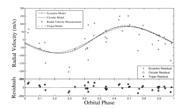
Bayesian model testing was also performed on the published radial velocity measurements (Lillo-Box et al., 2014; Barclay et al., 2014) in order to determine if a model that includes the radial velocity signal from a Trojan planet would be favored over a model that neglects a Trojan. Assumed quantities for these simulations include only the stellar mass (), and orbital period ( d) as opposed to the analysis performed by Lillo-Box et al. (2014), which assumed the eccentricity to be that which was estimated from their analysis of photometry. Based on model log-evidences, the eccentric one-planet model was slightly favored over the circular model by a Bayes’ factor of in agreement with the photometric results. The eccentric one-planet model predicts an eccentricity of , which is also in agreement (within uncertainty) with results presented in the previous section as well as the photometric analysis performed by Lillo-Box et al. (2013). This model also predicts a minimum planetary mass associated with Kepler-91b of , which along with the orbital inclination obtained from photometry, implies a true mass of , which is in agreement with the results from photometry. These two models were then tested against an eccentric two-planet model that assumes the second planet to be in the same orbit as the Jovian, but trailing it by a phase angle . This model was neither favored over nor rejected by the eccentric one-planet model. However, it is interesting that adding an additional two parameters to describe the hypothetical Trojan did not significantly change the log-evidence. The one-planet eccentric model yielded a higher log-evidence, with a difference in log-evidence between the two models being . It should also be noted that attempting to fit two radial velocity signals with the same period will result in significant degeneracies as can be seen in the semi-amplitudes estimated in Table 4. The predicted semi-amplitudes correspond to uncertainties in that are approximately of the mean value. However, this does not affect ones ability to perform Bayesian model testing. The two planet model also predicted a phase difference of . While the uncertainty here is large, this doesn’t rule out the expected phase difference for a Trojan of . These radial velocity measurements neither confirm or reject the Trojan hypothesis. In addition to comparing log-evidences, another common way to compare different models is to look at the value, which represents the sum of the squared residuals. Having the lowest , the two-planet model represents a better fit to the observed data. In a similar fashion, one may compare the log-likelihoods of a set of models, which describes the probability of observing a particular dataset given a set of model parameters. The higher the log-likelihood, the better the fit to the data. The two-planet model clearly has the highest maximum log-likelihood, but is not favored in log-evidence because the fit was not improved sufficiently to overcome the penalty of adding additional parameters to the model, which is taken into account when calculating the log-evidence.
| Two-Planet Model |
|
|
||||||
| Parameter | Kepler-91b | Trojan Candidate | Kepler-91b | Kepler-91b | ||||
| () | ||||||||
| () | … | |||||||
| … | ||||||||
| () | ||||||||
| () | ||||||||
| () | ||||||||
3.3 Stability of Trojan Configuration
In order to test the Trojan planet hypothesis further, a preliminary stability study was performed. One hundred () orbital configurations were generated by sampling the posterior obtained from the Kepler photometry. Initial conditions for each orbital configuration were determined by sampling from the posterior distributions obtained in the photometric two-planet simulations for , , , , , , and with the means and standard deviations being those that are listed in Table 3 for those that correspond to the photometric model parameters, and Table 1 for those which are previously published values. Each orbital configuration was tested for stability using the following cuts. The semi-major axes of the Jovian and hypothetical Trojan orbits cannot increase or decrease by more than 30% of the original value, the eccentricity of the orbits for either object cannot exceed one (), which would indicate a parabolic or hyperbolic trajectory, and the maximum allowed change in energy of the system was (Barnes and Quinn, 2004). The equations of motion for the three-body problem were integrated up to 50,000 days, which corresponds to approximately orbits of the Jovian and Trojan. All orbital configurations for the Trojan were found to be stable over this time period. Furthermore, the results predict librational periods of days and days, which both agree with the theoretical values predicted by equations (1) and (2). The relatively large uncertainties on these librational periods are likely due to the sampling of the initial conditions from the posterior. In the future longer integration times will be necessary to solidify the stability of such an orbital configuration.
3.4 Stability of Exomoon Configuration
A similar stability study was performed to investigate the exomoon hypothesis. Each parameter was again sampled from the posterior obtained from the photometric simulations. This excludes the mass and semi-major axis of the hypothesized exomoon since they were not modeled in the light curve. Due to the fact that the occultations associated with the hypothesized third body are observed in the light curve folded on the period of the Jovian, it would be reasonable to assume that the two bodies are in resonance. Therefore, the period of the exomoon was assumed to be , where ranges from in increments of and days. For each value of , orbital configurations were generated.
For an exomoon with mass , there were zero stable orbits for each value of . In the case of the 1:10 resonance, every configuration resulted in the moon crashing into the Jovian. For the 1:5 resonance, of the configurations resulted in the moon crashing into the Jovian, and resulted in the moon being expelled into a more distant orbit around the host star. The remaining configurations all resulted in the moon being shot out to more distant orbits around the host star, likely due to the fact that it’s semi-major axis was larger than the radius of the Hill sphere of the Jovian, which is approximated by
| (13) |
A moon that is outside of the Hill sphere of a planet, is not gravitationally bound to that planet. Based on the posterior estimates from photometry, the radius of the Hill sphere in the case of Kepler-91b is AU. This would translate to orbital periods for the moon of , which verifies the unstable behavior observed in the numerical simulations.
| Subset | (ppm) | (ppm) | |||
|---|---|---|---|---|---|
| Even - All Data | +11.5 | 4562.24 | |||
| Odd - All Data | - 1.5 | 4634.59 | |||
| Even - First Half | +13.9 | ||||
| Odd - First Half | -6.9 | ||||
| Even - Second Half | +3.2 | ||||
| Odd - Second Half | -0.6 |
3.5 Odd-Even Effects
and Systematic Noise
As shown in Figure 2, there are odd/even effects that appear in the light curve folded at twice the orbital period of the Jovian. These appear to occur halfway through the transit of the Jovian and apparent secondary of the Trojan (see Figure 2) and when binned at the Kepler cadence and folded on the accepted period of the Jovian apparently disappear. To test whether or not these are significant in affecting the model testing results, we tested the one-planet model against the two-planet model using six different subsets of the entire time-series. The subsets were defined as follows: the even/odd periods of the Jovian over the all quarters, the even/odd periods of the Jovian over the first eight quarters, and the even/odd periods of the Jovian over the last eight quarters for a total of six subsets. Results are displayed in Table 5.
Positive differences in the log-evidences indicate that the two-planet model is favored over the one-planet, whereas negative differences indicate that the one-planet model is favored. Clearly the odd/even effects are influencing the model testing results, since the two-planet model is favored over the one-planet model in the even periods, but not in the odd periods. This is also apparent in the model fits as the minimum chi-squared values (bolded in Table 5) alternate between even and odd periods. Since the libration period is estimated to be on the order of the orbital period of the Jovian, it is unlikely that the libration of a Trojan companion could explain this result. It is very possible that there is an unmodeled stellar effect or star-planet interaction that is responsible for these odd/even differences. The maximum log-likelihoods for each model are also listed in Table 5. Unlike the chi-squared values, these do not alternate between odd and even periods likely due to the fact that there are free parameters affecting the likelihood function. Namely the standard deviation of the noise, , and the correlation coefficient, . The one-planet model has fewer degrees of freedom compared to the two-planet model. As such there may be features in the data that the model cannot fit, and thus treats as noise by altering the estimated parameters that correspond to the likelihood function.
Since there is suspected to be a significant amount of systematic noise in the light curve of Kepler-91b, these extra dimming events may be caused by some unknown systematic effect(s). If the signal in the phase-folded light curve is truly from a Trojan companion, one should only rarely see similar dimming events (in depth and duration), when the light curve is folded on other random periods.
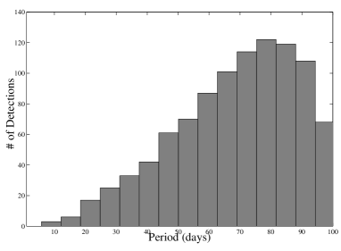
A transit detection routine was created to search for such eclipses and determine their frequency at various periods. First, the signal from the Jovian was subtracted from the light curve using the best-fit model from the photometric analysis in Section 3.1. Then, the residuals corresponding to the intervals over which the Jovian was in transit and when it was in secondary eclipse were removed. These residuals were then folded on random periods ranging from [0,100] days. Detections were deemed to have occured if the data points dipped below the mean of the entire dataset, at which time the area under the curve would be computed. A larger transit would correspond to a smaller, more negative, area under the curve. If any detections corresponded to a greater area under the curve than the apparent Trojan signal (), it would be discarded. In addition, if any events were found to have durations inconsistent with the apparent Trojan signal they would also we discarded. The apparent Trojan eclipse has a duration of approximately days. Events would be deemed detections if they had durations of days. This process was repeated for random periods. Figure 7 displays six examples of the detected dimming events as well as the apparent Trojan signal. Each window displays only part of the phase-folded residual as these detections often have durations much smaller than the phase as shown in Figure 8, dimming events similar to that associated with the hypothetical Trojan were more readily discovered at longer periods. While only four were detected around the orbital period of the Jovian, they were nevertheless detected making the systematic noise a serious candidate to explain the extra dimming.
4 Discussion
Presented here is a re-analysis of the Kepler-91 system. The results from the one-planet model for both photometry and radial velocity measurements re-confirm the planetary nature of the companion, Kepler-91b, as a hot-Jupiter with characteristics similar to those estimated by Lillo-Box et al. (2014). Based on the model log-evidence calculations, Kepler-91b is considerably more likely to be in an eccentric orbit, rather than circular, which is consistent with previous results. The estimate of the day-side temperature is consistent with the equilibrium temperature of the planet, although a possible confounding effect is that of the mid-eclipse brightening event that occurs during the secondary eclipse of Kepler-91b. The predicted albedo is also consistent for short-period hot-Jupiters (Angerhausen et al., 2014).
The Trojan planet hypothesis was tested by applying a two-planet model (Planet+Trojan, eccentric) to the Kepler photometric data that aims to describe Kepler-91b and a hypothetical Trojan planet. This two-planet model was signicantly favored over the one-planet model by a Bayes’ factor of , but was neither ruled out (nor verified) by the RV data obtained by Lillo-Box et al. (2014). When performing Bayesian model testing, there are two important factors: the ratio of the prior probabilities of the models and the ratio of the evidences of the data. When the prior probabilities of the models are assumed to be equal one can focus on the ratio of the evidences, or equivalently, the difference between their logarithms (the log odds ratio) (Knuth et al., 2015). In the analysis presented here, we focused on the differences between the logarithms of the evidence, which implicitly assumes that the prior probabilities of the models are equal. However, this assumption is questionable since our experience to date does not lead us to truly believe that it is as likely for Kepler-91 to have a Jovian planet as it is for Kepler-91 to have a Jovian planet with a Trojan companion. The log evidences must be compared with this in mind. Statistical evidence for the existence of Trojan planets has been uncovered (Hippke and Angerhausen, 2015). However, given that at present there are about exoplanet candidates and a Trojan companion to a planet has yet to be found, one could crudely estimate the ratio of probabilities to be something one the order of against the Jovian+Trojan model, which corresponds to a log probability of about . Thus one would not be confident in such assertions unless the log evidence in support of a Trojan was proportionately higher. The fact that the log-evidence differences supporting a Trojan is on the order of (see Section 3.1) yields an overall support with a probability on the order of .
Based on the model log-evidences for the single-planet case, we re-confirm the planetary nature of Kepler-91b with an estimated minimum mass of , which corresponds to a true mass of given the orbital inclination of determined using the photometric data. This estimate of the mass of Kepler-91b is consistent with the analysis of photometric data performed in Section 3.1, along with the results from Lillo-Box et al. (2014). The eccentricity of the orbit was found to be , which also agrees with the photometric analysis within uncertainty. Applying the two-planet (Planet + Trojan) model did not confirm or reject the Trojan hypothesis based on model log-evidences, however the two-planet model did have the lowest value, and highest log-likelihood making it a better fit to the data than the other models despite the Bayesian evidence being slightly lower than the one-planet eccentric model.
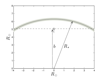
The Jovian + Trojan model provides similar estimates of the Kepler-91b parameters again supporting the idea that the planet is a hot Jupiter with mass , radius , albedo and day- and night-side temperatures of K and K, respectively. The day- and night-side temperatures of Kepler-91b in this model are equal to within uncertainty, and consistent with the expected equilibrium temperature of the planet suggesting that it may have high winds that equilibrate its day and night sides. Results also suggest that a Trojan would be sub-Neptunian, with a radius , and with a mass of . The mass was not well estimated in this case because of the apparent lack of Doppler boosting and ellipsoidal variations associated with this object. The day and night-side temperatures were determined to be a scorching K and K, respectively. While the uncertainty in these estimates are such that the temperatures are not conclusive, it is possible, according to the model, that the day-side of the planet may be greater than or approximately equal to the effective temperature of the host star, which has been determined to be (Lillo-Box et al., 2013)). The two-planet model fit illustrated in Figure 6 shows the comparatively small depth of the Trojan transit to the corresponding secondary eclipse. While this significant disparity in transit and secondary eclipse depths is apparent in the underlying data, and supportive of an extremely high day-side temperature, the particular values of the estimates could be affected by the mid-transit and mid-eclipse brightening events, which are neither modeled nor well-understood. In addition, there are other known effects, which are not presently accounted for by EXONEST that could result in increased temperature estimates. These include the extra illumination of the side of the planet opposite the star due to the planet’s proximity (see for example, Figure 10 in Lillo-Box et al. (2013)) in addition to the high inclination of the orbit, which would allow part of the day-side of the planet to be visible from Earth during transit. Also, a highly inclined and slightly eccentric orbit has a high probability to produce a grazing transit (see for example WASP-67; Hellier et al. (2012)). However, using posterior estimates of the planetary radius and inclination (Table 3) along with the published values of the stellar radius and semi-major axis (Table 1), one can calculate the estimated impact parameter, . Figure 9 displays the sky-projected distance between the center of the host star and the center of the planet, which shows that Kepler-91b is most likely not in a grazing orbit.
In addition, if a Trojan companion were present, both the Jovian and Trojan would undergo librations as discussed in Sections 1.1 and 3.3. Our simulations, based on the current model parameter estimates, show that the orbital phase of the Jovian planet would not significantly vary, whereas the Trojan’s phase would vary. One would expect that this would result in a smearing of the Trojan transit in the phase-folded light curve. To properly model the system, N-body fitting routines should be employed rather than the Keplerian fitting used here. While the libration periods obtained from our current model parameter estimates do not seem to be able to explain the observed even/odd period effects, a carefully modeling of the planet-planet interactions could account for additional unusual features observed in the light curve, such as the mideclipse brightening events.
Given the available data and the models employed, it is not yet possible to come to a conclusion as to the presence of a Trojan partner to Kepler-91b. In favor of the Trojan hypothesis is the fact that the Bayesian evidence of the Jovian+Trojan model is times greater than the Jovian model. This hypothesis is still highly probable if one considers a reasonable prior probability reflecting the fact that a Trojan planet has never been observed in the set of or so exoplanet candidates111Trojans have however been observed in our solar system at the Lagrange points of Venus, Earth, Mars, Jupiter, Uranus, and Neptune. In addition, Saturn’s moon’s Tethys and Dione each have two Trojan moons.. It is also remarkable that the model selected the appropriate relative phase for the Trojan companion. While the probability of this occurring is not overwhelming, it is on the order of . However, this correct positioning of a Trojan occurred at the expense of having the secondary transit be deeper than the primary, which leads to the model ascribing an unphysically high day-side temperature to the Trojan, which clearly makes the Trojan hypothesis suspect. In addition, unusual features, such as the odd/even phase differences in the light curve and the mid-eclipse brightening, which occurs not only during the Jovian eclipses, but also during hypothetical Trojan eclipses may be mimicking a Trojan-like signal. At this stage, given the available data and the models employed, it is impossible to say anything definitive concerning the presence of a Trojan companion.
5 Summary and Outlook
We were able to confirm the planetary nature of Kepler-91b using the EXONEST code for photometric analysis of its optical lightcurve obtained with the Kepler Space telescope and radial velocity analysis on data taken from the literature.
We find that introducing an additional object to the system can explain the extra dimming in the lightcurve: an EXONEST photometric model including an object in the same orbit as Kepler-91b, but shifted by degrees, produces a significantly higher Bayesian evidence than a model without this sub-Neptunian Trojan companion (see section 3.1). This model to describe the light curve is not ruled out by radial velocity, and the orbit seems to be stable over the course of 50,000 days, or 8000 cycles. On the other hand, this model also predicted an unphysical day-side temperature and a secondary eclipse depth greater than that of the transit, which would imply that either there are unknown heating mechanisms for such an object, or that it is a false-positive, which is far more likely.
We are able to exclude previously suggested alternative explanations such as the presence of a moon, a resonant outer planet or instrumental effect for the observed dimmings caused by the hypothetical Trojan (see section 1.2, 1.3 and 1.4). However, we detect a signficant odd/even effect in the phase-folded light curve, and similar dimming events in the light curve folded on randomized periods, both of which could mimic the hypothetical Trojan signal.
The Kepler-91 system is currently of great interest since it is a short-period hot-Jupiter orbiting a star in its red giant stage. If this Trojan planet is confirmed it would not only be the first detection of an exo-Trojan planet, but also would provide the unique opportunity to study two different worlds that are in identical stellar environments thus promising to provide insights into star-planet interactions.
Despite this comprehensive investigation of the potential Trojan companion, given the data at hand we cannot conclude that it is the cause of the extra dimming events observed in the Kepler light curve.
Acknowledgments
The authors acknowledge the efforts of the Kepler Mission team in obtaining the light curve data used in this publication. These data were generated by the Kepler Mission science pipeline through the efforts of the Kepler Science Operations Center and Science Office. The Kepler Mission is lead by the project office at NASA Ames Research Center. Ball Aerospace built the Kepler photometer and spacecraft which is operated by the mission operations center at LASP. These data products are archived at the Mikulski Archive for Space Telescopes.
The authors would thank the University at Albany Physics Department for its ongoing support in our exoplanet research.
Daniel Angerhausen’s Research was supported by an appointment to the NASA Postdoctoral Program at the Goddard Space Flight Center, administered by Oak Ridge Associated Universities through a contract with NASA.
The authors thank Em DeLarme, Jon Morse, William B. Rossow, and Barbara J. Thompson for discussions about this exciting extrasolar system.
References
- Angerhausen et al. [2014] D. Angerhausen, E. DeLarme, and J. A. Morse. A comprehensive study of Kepler phase curves and secondary eclipses–temperatures and albedos of confirmed Kepler giant planets. PASP (In Press), 2014.
- Barclay et al. [2014] T. Barclay, M. Endl, D. Huber, D. Foreman-Mackey, W. D. Cochran, P. J. MacQueen, J. F. Rowe, and E. V. Quintana. Radial velocity observations and light curve noise modeling confirm that Kepler-91b is a giant planet orbiting a giant star. arXiv preprint arXiv:1408.3149, 2014.
- Barnes and Quinn [2004] R. Barnes and T. Quinn. The (in) stability of planetary systems. The Astrophysical Journal, 611(1):494, 2004.
- Batalha et al. [2013] N. M. Batalha, J. F. Rowe, S. T. Bryson, T. Barclay, C. J. Burke, D. A. Caldwell, J. L. Christiansen, F. Mullally, S. E. Thompson, T. M. Brown, et al. Planetary candidates observed by Kepler. iii. analysis of the first 16 months of data. The Astrophysical Journal Supplement Series, 204(2):24, 2013.
- Borucki et al. [2009] W. J. Borucki, D. Koch, J. Jenkins, D. Sasselov, R. Gilliland, N. Batalha, D. W. Latham, D. Caldwell, G. Basri, T. Brown, and et al. Kepler’s optical phase curve of the exoplanet HAT-P-7b. Science, 325(5941):709–709, 2009.
- Caton et al. [2001] D. B. Caton, S. A. Davis, K. A. Kluttz, R. J. Stamilio, and K. D. Wohlman. Searching for extrasolar trojan planets: A status report. In AAS 198th Meeting, June 2001, page 69.01. 2001.
- Charbonneau et al. [2005] D. Charbonneau, L. E. Allen, S. T. Megeath, G. Torres, R. Alonso, T. M. Brown, R. L. Gilliland, D. W. Latham, G. Mandushev, F. T. O Donovan, et al. Detection of thermal emission from an extrasolar planet. The Astrophysical Journal, 626(1):523, 2005.
- Claret and Bloemen [2011] A. Claret and S. Bloemen. Gravity and limb-darkening coefficients for the Kepler, CoRoT, Spitzer, uvby, UBVRIJHK, and Sloan photometric systems. Astronomy and astrophysics, 529, 2011.
- Dvorak et al. [2004] R. Dvorak, E. Pilat-Lohinger, R. Schwarz, and F. Freistetter. Extrasolar trojan planets close to habitable zones. arXiv preprint astro-ph/0408079, 2004.
- Esteves et al. [2013] L. J. Esteves, E. J.W. De Mooij, and R. Jayawardhana. Optical phase curves of Kepler exoplanets. arXiv preprint arXiv:1305.3271, 2013.
- Faigler and Mazeh [2011] S. Faigler and T. Mazeh. Photometric detection of non-transiting short-period low-mass companions through the beaming, ellipsoidal and reflection effects in Kepler and CoRoT light curves. Monthly Notices of the Royal Astronomical Society, 415(4):3921–3928, 2011.
- Feroz et al. [2009] F. Feroz, M. P. Hobson, and M. Bridges. Multinest: an efficient and robust Bayesian inference tool for cosmology and particle physics. Monthly Notices of the Royal Astronomical Society, 398(4):1601–1614, 2009.
- Feroz et al. [2011] F. Feroz, S. T. Balan, and M. P. Hobson. Detecting extrasolar planets from stellar radial velocities using Bayesian evidence. Monthly Notices of the Royal Astronomical Society, 415(4):3462–3472, 2011.
- Feroz et al. [2013] F. Feroz, M. P. Hobson, E. Cameron, and A. N. Pettitt. Importance nested sampling and the multinest algorithm. arXiv preprint arXiv:1306.2144, 2013.
- Ford and Gaudi [2006] E. B. Ford and B. S. Gaudi. Observational constraints on trojans of transiting extrasolar planets. The Astrophysical Journal Letters, 652(2):L137, 2006.
- Ford and Holman [2007] E. B. Ford and M. J. Holman. Using transit timing observations to search for trojans of transiting extrasolar planets. The Astrophysical Journal Letters, 664(1):L51, 2007.
- Hellier et al. [2012] C. Hellier, D. R. Anderson, A. C. Cameron, A. P. Doyle, A. Fumel, M. Gillon, E. Jehin, M. Lendl, P. F. L. Maxted, F. Pepe, et al. Seven transiting hot jupiters from wasp-south, euler and trappist: Wasp-47b, wasp-55b, wasp-61b, wasp-62b, wasp-63b, wasp-66b and wasp-67b. Monthly Notices of the Royal Astronomical Society, 426(1):739–750, 2012.
- Hippke and Angerhausen [2015] M. Hippke and D. Angerhausen. A statistical search for a population of exo-trojans in the kepler dataset. The Astrophysical Journal, 2015.
- Jenkins and Doyle [2003] J. M. Jenkins and L. R. Doyle. Detecting reflected light from close-in extrasolar giant planets with the Kepler photometer. The Astrophysical Journal, 595(1):429, 2003.
- Jenkins et al. [2010] J. M. Jenkins, D. A. Caldwell, H. Chandrasekaran, J. D. Twicken, S. T. Bryson, E. V. Quintana, B. D. Clarke, J. Li, C. Allen, P. Tenenbaum, et al. Overview of the Kepler science processing pipeline. The Astrophysical Journal Letters, 713(2):L87, 2010.
- Knuth et al. [2012] K. H. Knuth, B. Placek, and Z. Richards. Detection and characterization of non-transiting extra-solar planets in Kepler data using reflected light variations. In Intelligent Data Understanding (CIDU), 2012 Conference on, pages 31–38. IEEE, 2012.
- Knuth et al. [2015] K. H. Knuth, M. Habeck, N. K. Malakar, A. M. Mubeen, and B. Placek. Evidence and model selection. YDSPR, 2015.
- Lillo-Box et al. [2013] J. Lillo-Box, D. Barrado, A. Moya, B. Montesinos, J. Montalbán, A. Bayo, M. Barbieri, C. Régulo, L. Mancini, H. Bouy, et al. Kepler-91b: a planet at the end of its life. planet and giant host star properties via light-curve variations. arXiv preprint arXiv:1312.3943, 2013.
- Lillo-Box et al. [2014] J. Lillo-Box, D. Barrado, T. H. Henning, L. Mancini, S. Ciceri, P. Figueira, N. C. Santos, J. Aceituno, and S. Sánchez. Radial velocity confirmation of Kepler-91 b-additional evidence of its planetary nature using the calar alto/cafe instrument. Astronomy & Astrophysics, 568:L1, 2014.
- Loeb and Gaudi [2003] A. Loeb and S. B. Gaudi. Periodic flux variability of stars due to the reflex Doppler effect induced by planetary companions. The Astrophysical Journal Letters, 588(2):L117, 2003.
- Madhusudhan and Winn [2009] N. Madhusudhan and J. N. Winn. A search for exotrojans in transiting exoplanetary systems. In F. Pont, D. Sasselov, and M. J. Holman, editors, IAU Symposium, volume 253 of IAU Symposium, pages 496–498, February 2009. 10.1017/S1743921308027038.
- Metropolis et al. [1953] N. Metropolis, A. W. Rosenbluth, M. N. Rosenbluth, A. H. Teller, and E. Teller. Equation of state calculations by fast computing machines. The journal of chemical physics, 21(6):1087–1092, 1953.
- Otten and van Ginneken [1989] R. Otten and L. van Ginneken. The annealing algorithm. Kluwer, BV, 1989.
- Perryman [2011] M. Perryman. The exoplanet handbook. Cambridge University Press, 2011.
- Placek et al. [2013] B. Placek, Z. Richards, and K. H. Knuth. Detecting non-transiting exoplanets. In Bayesian Inference and Maximum Entropy Methods in Science and Engineering: 32nd International Workshop on Bayesian Inference and Maximum Entropy Methods in Science and Engineering, volume 1553, pages 23–29. AIP Publishing, 2013.
- Placek et al. [2014] B. Placek, K. H. Knuth, and D. Angerhausen. Exonest: Bayesian model selection applied to the detection and characterization of exoplanets via photometric variations. The Astrophysical Journal, 795(2), 2014. arXiv preprint arXiv:1310.6764.
- Rogers [2014] L. A. Rogers. Most 1.6 earth-radius planets are not rocky. arXiv preprint arXiv:1407.4457, 2014.
- Rybicki and Lightman [2008] G. B. Rybicki and A. P. Lightman. Radiative processes in astrophysics. John Wiley & Sons, 2008.
- Schwarz et al. [2007] R. Schwarz, R. Dvorak, Á. Süli, and B. Érdi. Survey of the stability region of hypothetical habitable trojan planets. Astronomy and Astrophysics-Berlin then Les Ulis, 474(3):1023, 2007.
- Schwarz et al. [2009] R. Schwarz, Á. Süli, and R. Dvorak. Dynamics of possible trojan planets in binary systems. MNRAS, 398(4):2085–2090, 2009. 10.1111/j.1365-2966.2009.15248.x.
- Seager [2010] S. Seager. Exoplanet atmospheres: physical processes. Princeton University Press, 2010.
- Seager et al. [2000] S. Seager, B. A. Whitney, and D. D. Sasselov. Photometric light curves and polarization of close-in extrasolar giant planets. The Astrophysical Journal, 540(1):504, 2000.
- Shporer et al. [2011] A. Shporer, J. M. Jenkins, J. F. Rowe, D. T. Sanderfer, S. E. Seader, J. C. Smith, M. D. Still, S. E. Thompson, J. D. Twicken, and W. F. Welsh. Detection of KOI-13.01 using the photometric orbit. The Astronomical Journal, 142(6):195, 2011.
- Sivia and Skilling [2006] D. Sivia and J. Skilling. Data analysis: a Bayesian tutorial. Oxford University Press, USA, 2006.
- Skilling et al. [2006] J. Skilling et al. Nested sampling for general Bayesian computation. Bayesian Analysis, 1(4):833–859, 2006.
- Sliski and Kipping [2014] D. H. Sliski and D. M. Kipping. A high false positive rate for Kepler planetary candidates of giant stars using asterodensity profiling. The Astrophysical Journal, 788(2):148, 2014.
- Smith et al. [2012] J. C. Smith, M. C. Stumpe, J. E. Van Cleve, J. M. Jenkins, T. S. Barclay, M. N. Fanelli, F. R. Girouard, J. J. Kolodziejczak, S. D. McCauliff, R. L. Morris, et al. Kepler presearch data conditioning ii-a Bayesian approach to systematic error correction. Publications of the Astronomical Society of the Pacific, 124(919):1000–1014, 2012.
- Spiegel and Madhusudhan [2012] D. S. Spiegel and N. Madhusudhan. Jupiter will become a hot jupiter: Consequences of post-main-sequence stellar evolution on gas giant planets. The Astrophysical Journal, 756(2):132, 2012.
- Stumpe et al. [2014] M. C. Stumpe, J. C. Smith, J. H. Catanzarite, J. E. Van Cleve, J. M. Jenkins, J. D. Twicken, and F. R. Girouard. Multiscale systematic error correction via wavelet-based bandsplitting in Kepler data. Publications of the Astronomical Society of the Pacific, 126:100–114, 2014.
- Twicken et al. [2010] J. D. Twicken, B. D. Clarke, S. T. Bryson, P. Tenenbaum, H. Wu, J. M. Jenkins, F. Girouard, and T. C. Klaus. Photometric analysis in the Kepler science operations center pipeline. In SPIE Astronomical Telescopes+ Instrumentation, pages 774023–774023. International Society for Optics and Photonics, 2010.