Efficient Algorithms with Asymmetric Read and Write Costs

Abstract

In several emerging technologies for computer memory (main memory), the cost of reading is significantly cheaper than the cost of writing. Such asymmetry in memory costs poses a fundamentally different model from the RAM for algorithm design. In this paper we study lower and upper bounds for various problems under such asymmetric read and write costs. We consider both the case in which all but $O(1)$ memory has asymmetric cost, and the case of a small cache of symmetric memory. We model both cases using the $(M,\omega)$-ARAM, in which there is a small (symmetric) memory of size $M$ and a large unbounded (asymmetric) memory, both random access, and where reading from the large memory has unit cost, but writing has cost $\omega\gg 1$.

For FFT and sorting networks we show a lower bound cost of $\Omega(\omega n\log_{\omega M}n)$, which indicates that it is not possible to achieve asymptotic improvements with cheaper reads when $\omega$ is bounded by a polynomial in $M$. Moreover, there is an asymptotic gap (of $\min(\omega,\log n)/\log(\omega M)$) between the cost of sorting networks and comparison sorting in the model. This contrasts with the RAM, and most other models, in which the asymptotic costs are the same. We also show a lower bound for computations on an $n\times n$ diamond DAG of $\Omega(\omega n^{2}/M)$ cost, which indicates no asymptotic improvement is achievable with fast reads. However, we show that for the minimum edit distance problem (and related problems), which would seem to be a diamond DAG, we can beat this lower bound with an algorithm with only $O(\omega n^{2}/(M\min(\omega^{1/3},M^{1/2})))$ cost. To achieve this we make use of a “path sketch” technique that is forbidden in a strict DAG computation. Finally, we show several interesting upper bounds for shortest path problems, minimum spanning trees, and other problems. A common theme in many of the upper bounds is that they require redundant computation and a tradeoff between reads and writes.

1 Introduction

Fifty years of algorithms research has focused on settings in which reads and writes (to memory) have similar cost. But what if reads and writes to memory have significantly different costs? How would that impact algorithm design? What new techniques are useful for trading-off doing more cheaper operations (say more reads) in order to do fewer expensive operations (say fewer writes)? What are the fundamental limitations on such trade-offs (lower bounds)? What well-known equivalences for traditional memory fail to hold for asymmetric memories?

Such questions are coming to the fore with the arrival of new main-memory technologies [30, 33] that offer key potential benefits over existing technologies such as DRAM, including nonvolatility, signicantly lower energy consumption, and higher density (more bits stored per unit area). These emerging memories will sit on the processor’s memory bus and be accessed at byte granularity via loads and stores (like DRAM), and are projected to become the dominant main memory within the decade [37, 50]. Because these emerging technologies store data as “states” of a given material, the cost of reading (checking the current state) is significantly cheaper than the cost of writing (modifying the physical state of the material): Reads are up to an order of magnitude or more lower energy, lower latency, and higher (per-module) bandwidth than writes [5, 6, 9, 10, 19, 20, 31, 32, 34, 42, 48].

This paper provides a first step towards answering these fundamental questions about asymmetric memories. We introduce a simple model for studying such memories, and a number of new results. In the simplest model we consider, there is an asymmetric random-access memory such that reads cost 1 and writes cost $\omega\gg 1$, as well as a constant number of symmetric “registers” that can be read or written at unit cost. More generally, we consider settings in which the amount of symmetric memory is $M\ll n$, where $n$ is the input size: We define the $(M,\omega)$-Asymmetric RAM (ARAM), comprised of a symmetric small-memory of size $M$ and an asymmetric large-memory of unbounded size with write cost $\omega$. The ARAM cost $Q$ is the number of reads from large-memory plus $\omega$ times the number of writes to large-memory. The time $T$ is $Q$ plus the number of reads and writes to small-memory.

Table 1: Summary of Our Results for the $(M,\omega)$-ARAM (^†indicates main results)

problem	ARAM cost	time	section
	$Q(n)$ or $Q(n,m)$	$T(n)$ or $T(n,m)$
FFT	$\Theta(\omega n\log n/\log(\omega M))^{\dagger}$	$\Theta(Q(n)+n\log n)$	3, 4
sorting networks	$\Omega(\omega n\log n/\log(\omega M))^{\dagger}$	$\Omega(Q(n)+n\log n)$	3
sorting (comparison)	$O(n(\log n+\omega))$	$\Theta(n(\log n+\omega))$	4, [9]
diamond DAG	$\Theta(n^{2}\omega/M)^{\dagger}$	$\Theta(Q(n)+n^{2})$	3
longest common subsequence, edit distance	$O(n^{2}\omega/\min(\omega^{1/3}M,M^{3/2}))^{\dagger}$	$O(n^{2}(1+\omega/\min(\omega^{1/3}M^{2/3},M^{3/2})))^{\dagger}$	5
search tree, priority queue	$O(\omega+\log n)$ per update	$O(\omega+\log n)$ per update	4
2D convex hull, triangulation	$O(n(\log n+\omega))$	$\Theta(n(\log n+\omega))$	4
BFS, DFS, topological sort,	$\Theta(\omega n+m)$	$\Theta(\omega n+m)$	4
biconnected components, SCC
single-source shortest path	$O(\min(n(\omega+m/M),(m+n\log n)\omega,m(\omega+\log n)))^{\dagger}$	$O(Q(n,m)+n\log n)$	6
all-pairs shortest-path	$O(n^{2}(\omega+n/\sqrt{M}))$	$O(Q(n)+n^{3})$	4
minimum spanning tree	$O(m\min(\log n,n/M)+\omega n)^{\dagger}$	$O(Q(n,m)+n\log n)$	7

We present a number of lower and upper bounds for the $(M,\omega)$-ARAM, as summarized in Table 1. These results consider a number of fundamental problems and demonstrate how the asymptotic algorithm costs decrease as a function of $M$, e.g., polynomially, logarithmically, or not at all.

For FFT we show an $\Omega(\omega n\log_{\omega M}n)$ lower bound on the ARAM cost, and a matching upper bound. Thus, even allowing for redundant (re)computation of nodes (to save writes), it is not possible to achieve asymptotic improvements with cheaper reads when $\omega\in O(M^{c})$ for a constant $c$. Prior lower bound approaches for FFTs for symmetric memory fail to carry over to asymmetric memory, so a new lower bound technique is required. We use an interesting new accounting argument for fractionally assigning a unit weight for each node of the network to subcomputations that each have cost $\omega M$. The assignment shows that each subcomputation has on average at most $M\log(\omega M)$ weight assigned to it, and hence the total cost across all $\Theta(n\log n)$ nodes yields the lower bound.

For sorting, we show the surprising result that on asymmetric memories, comparison sorting is asymptotically faster than sorting networks. This contrasts with the RAM model (and I/O models, parallel models such as the PRAM, etc.), in which the asymptotic costs are the same! The lower bound leverages the same key partitioning lemma as in the FFT proof.

We present a tight lower bound for DAG computation on diamond DAGs that shows there is no asymptotic advantage of cheaper reads. On the other hand, we also show that allowing a vertex to be “partially” computed before all its immediate predecessors have been computed (thereby violating a DAG computation rule), we can beat the lower bound and show asymptotic advantage. Specifically, for both the longest common subsequence and edit distance problems (normally thought of as diamond DAG computations), we devise a new “path sketch” technique that leverages partial aggregation on the DAG vertices. Again we know of no other models in which such techniques are needed.

Finally, we show how to adapt Dijkstra’s single-source shortest-paths algorithm using phases so that the priority queue is kept in small-memory, and briefly sketch how to adapt Borůvka’s minimum spanning tree algorithm to reduce the number of shortcuts and hence writes that are needed. A common theme in many of our algorithms is that they use redundant computations and require a tradeoff between reads and writes.

Related Work

Prior work [7, 21, 25, 38, 39, 47] has studied read-write asymmetries in NAND flash memory, but this work has focused on (i) the asymmetric granularity of reads and writes in NAND flash chips: bits can only be cleared by incurring the overhead of erasing a large block of memory, and/or (ii) the asymmetric endurance of reads and writes: individual cells wear out after tens of thousands of writes to the cell. Emerging memories, in contrast, can read and write arbitrary bytes in-place and have many orders of magnitude higher write endurance, enabling system software to readily balance application writes across individual physical cells by adjusting its virtual-to-physical mapping. Other prior work has studied database query processing under asymmetric read-write costs [11, 12, 46, 47] or looked at other systems considerations [13, 31, 36, 49, 51, 52]. Our recent paper [9] introduced the general study of parallel (and external memory) models and algorithms with asymmetric read and write costs, focusing on sorting. Our follow-on paper [8] defined an abstract nested-parallel model of computation with asymmetric read-write costs that maps efficiently onto more concrete parallel machine models using a work-stealing scheduler, and presented reduced-write, work-efficient, highly-parallel algorithms for a number of fundamental problems such as tree contraction and convex hull. In contrast, this paper considers a much simpler model (the sequential $(M,\omega)$-ARAM) and presents not just algorithms but also lower bounds—plus, the techniques are new. Finally, concurrent with this paper, Carson et al. [10] developed interesting upper and lower bounds for various linear algebra problems and direct N-body methods under asymmetric read and write costs. For sequential algorithms, they define a model similar to the $(M,\omega)$-ARAM (as well as a cache-oblivious variant), and show that for “bounded data reuse” algorithms, i.e., algorithms in which each input or computed value is used only a constant number of times, the number of writes to asymmetric memory is asymptotically the same as the sum of the reads and writes to asymmetric memory. This implies, for example, a tight $\Omega(n\log n/\log M)$ lower bound on the number of writes for FFT under the bounded data reuse restriction; in contrast, our tight bounds for FFT do not have this restriction and use fewer writes. They also presented algorithms without this restriction for matrix multiplication, triangular solve, and Cholesky factorization that reduce the number of writes to $\Theta(\mbox{output size})$, without increasing the number of reads, as well as various distributed-memory parallel algorithms.

2 Model and Preliminaries

We analyze algorithms in an $(M,\omega)$-ARAM. In the model we assume a symmetric small-memory of size $M\geq 1$, an asymmetric large-memory of unbounded size, and a write cost $\omega\geq 1$, which we assume without loss of generality is an integer. (Typically, we are interested in the setting where $n\gg M$, where $n$ is the input size, and $\omega\gg 1$.) We assume standard random access machine (RAM) instructions. We consider two cost measures for computations in the model. We define the (asymmetric) ARAM cost $Q$ as the total number of reads from large-memory plus $\omega$ times the number of writes to large-memory. We define the (asymmetric) time $T$ as the ARAM cost plus the number of reads from and writes to small-memory. Because all instructions are from memory, this includes any cost of computation. In the paper we present results for both cost measures.

The model contrasts with the widely-studied external-memory model [1] in the asymmetry of the read and write costs. Also for simplicity in this paper we do not partition the memory into blocks of size $B$. Another difference is that the asymmetry implies that even the case of $M=O(1)$ (studied in [9] for sorting) is interesting. We note that our ARAM cost is a special case of the general flash model cost proposed in [4]; however that paper presents algorithms only for another special case of the model with symmetric read-write costs.

We use the term value to refer to an object that fits in one word (location) of the memory. We assume words are of size $\Theta(\log n)$ for input size $n$. The size $M$ is the number of words in small-memory. All logarithms are base 2 unless otherwise noted. The DAG computation problem is given a DAG and a value for each of its input vertices (in-degree = 0), compute the value for each of its output vertices (out-degree = 0). The value of any non-input vertex can be computed in unit time given the value of all its immediate predecessors. As in standard I/O models [1] we assume values are atomic and cannot be split when mapped into the memory. The DAG computation problem can be modeled as a pebbling game on the DAG [29]. Note that we allow (unbounded) recomputation of a DAG vertex, and indeed recomputation is a useful technique for reducing the number of writes (at the cost of additional reads).

3 Lower Bounds

We start by showing lower bounds for FFT DAGs, sorting networks and diamond DAGs. The idea in showing the lower bounds is to partition a computation into subcomputations that each have a lower bound on cost, but an upper bound on the number of inputs and outputs they can use. Our lower bound for FFT DAGs then uses an interesting accounting technique that gives every node in the DAG a unit weight, and fractionally assigns this weight across the subcomputations. In the special case $\omega=1$, this leads to a simpler proof for the lower bound on the I/O complexity of FFT DAGs than the well-known bound by Hong and Kung [28].

We refer to a subcomputation as any contiguous sequence of instructions. The outputs of a subcomputation are the values written by the subcomputation that are either an output of the full computation or read by a later subcomputation. Symmetrically, the inputs of a subcomputation are the values read by the subcomputation that are either an input of the full computation or written by a previous subcomputation. The space of a computation or subcomputation is the number of memory locations both read and written. An $(l,m)$-partitioning of a computation is a partitioning of instructions into subcomputations such that each has at most $l$ inputs and at most $m$ outputs. We allow for recomputation—instructions in different subcomputations might compute the same value.

Lemma 1.

Any computation in the $(M,\omega)$-ARAM has an $((\omega+1)M,2M)$-partitioning such that at most one of the subcomputations has ARAM cost $Q<\omega M$.

Proof.

We generate the partitioning constructively. Starting at the beginning, partition the instructions into contiguous blocks such that all but possibly the last block has cost $Q\geq\omega M$, but removing the last instruction from the block would have cost $Q<\omega M$. To remain within the cost bound each such subcomputation can read at most $\omega M$ values from large-memory. It can also read the at most $M$ values that are in the small-memory when the subcomputation starts. Therefore it can read at most $(\omega+1)M$ distinct values from the input or from previous subcomputations. Similarly, each subcomputation can write at most $M$ values to large-memory, and an additional $M$ that remain in small-memory when the subcomputation ends. Therefore it can write at most $2M$ distinct values that are available to later subcomputations or the output. ∎

FFT. We now consider lower bounds for the DAG computation problem for the family of FFT DAGs (also called FFT networks, or butterfly networks). The FFT DAG of input size $n=2^{k}$ consists of $k+1$ levels each with $n$ vertices (total of $n\log 2n$ vertices). Each vertex $(i,j)$ at level $i\in{0,\ldots,k-1}$ and row $j$ has two out edges, which go to vertices $(i+1,j)$ and $(i+1,j\oplus 2^{i})$ ($\oplus$ is the exclusive-or of the bit representation). This is the DAG used by the standard FFT (Fast Fourier Transform) computation. We note that in the FFT DAG there is at most a single path from any vertex to another.

Lemma 2.

Any $(l,m)$-partitioning of a computation for simulating an $n$ input FFT DAG has at least $n\log n/(m\log l)$ subcomputations.

Proof.

We refer to all vertices whose values are outputs of any subcomputation, as partition output vertices. We assign each such vertex arbitrarily to one of the subcomputations for which it is an output.

Consider the following accounting scheme for fractionally assigning a unit weight for each non-input vertex to some set of partition output vertices. If a vertex is a partition output vertex, then assign the weight to itself. Otherwise take the weight, divide it evenly between its two immediate descendants (out edges) in the FFT DAG, and recursively assign that weight to each. For example, for a vertex $x$ that is not a partition output vertex, if an immediate descendant $y$ is a partition output vertex, then $y$ gets a weight of $1/2$ from $x$, but if not and one of $y$’s immediate descendants $z$ is, then $z$ gets a weight of $1/4$ from $x$. Since each non-input vertex is fully assigned across some partition output vertices, the sum of the weights assigned across the partition output vertices exactly equals $|V|-n=n\log n$. We now argue that every partition output vertex can have at most $\log l$ weight assigned to it. Looking back from an output vertex we see a binary tree rooted at the output. If we follow each branch of the tree until we reach an input for the subcomputation, we get a tree with at most $l$ leaves, since there are at most $l$ inputs and at most a single path from every vertex to the output. The contribution of each vertex in the tree to the output is $1/2^{i}$, where $i$ is its depth (the root is depth $0$). The leaves (subcomputation inputs) are not included since they are partition output vertices themselves, or inputs to the whole computation, which we have excluded. By induction on the tree structure, the weight of that tree is maximized when it is perfectly balanced, which gives a total weight of $\log l$.

Therefore since every subcomputation can have at most $m$ outputs, the total weight assigned to each subcomputation is at most $m\log l$. Since the total weight across all subcomputations is $n\log n$, the total number of subcomputations is at least $n\log n/(m\log l)$. ∎

Theorem 1 (FFT Lower Bound).

Any solution to the DAG computation problem on the family of FFT DAGs parametrized by input size $n$ has costs $\displaystyle Q(n)=\Omega\mathopen{}\mathclose{{}\left({\omega n\log n}/{\log(\omega M)}}\right)$ and $T(n)=\Omega(Q(n)+n\log n)$ on the $(M,\omega)$-ARAM.

Proof.

By Lemma 1 every computation must have an $((\omega+1)M,2M)$-partitioning with subcomputation cost $Q\geq\omega M$ (except perhaps one). Plugging in Lemma 2 we have $Q(n)\geq\omega Mn\log n/(2M\log((\omega+1)M))$, which gives our bound on $Q(n)$. For $T(n)$ we just add in the cost of the computation of each vertex. ∎

Note that whichever of $\omega$ and $M$ is larger will dominate in the denominator of $Q(n)$. When $\omega\leq M$, these lower bounds match those for the standard external memory model [28, 1] assuming both reads and writes have cost $\omega$. This implies that cheaper reads do not help asymptotically in this case. When $\omega>M$, however, there is a potential asymptotic advantage for the cheaper reads.

Sorting Networks. A sorting network is a acyclic network of comparators, each of which takes two input keys and returns the minimum of the keys on one output, and the maximum on the other. For a family of sorting networks parametrized by $n$, each network takes $n$ inputs, has $n$ ordered outputs, and when propagating the inputs to the outputs must place the keys in sorted order on the outputs. A sorting network can be modeled as a DAG in the obvious way. Ajtai, Komlós and Szemerédi [3] described a family of sorting networks that have size $O(n\log n)$ and depth $O(\log n)$. Their algorithm is complicated and the constants are very large. Many simplifications and constant factor improvements have been made, including the well known Patterson variant [41] and a simplification by Seiferas [44]. Recently Goodrich [26] gave a much simpler construction of an $O(n\log n)$ size network, but it requires polynomial depth. Here we show lower bounds of simulating any sorting network on the $(M,\omega)$-ARAM.

Theorem 2 (Sorting Lower Bound).

Simulating any family of sorting networks parametrized on input size $n$ has $\displaystyle Q(n)=\Omega\mathopen{}\mathclose{{}\left(\frac{\omega n\log n}{\log(\omega M)}}\right)$ and $T(n)=\Omega(Q(n)+n\log n)$ on the $(M,\omega)$-ARAM.

Proof.

Consider an $(l,m)$-partitioning of the computation. Each subcomputation has at most $l$ inputs from the network, and $m$ outputs for the network. The computation is oblivious to the values in the network (it can only place the min and max on the outputs of each comparator). Therefore locations of the inputs and outputs are fixed independent of input values. The total number of choices the subcomputation has is therefore $\binom{l}{m}m!=l!/(l-m)!<l^{m}$. Since there are $n!$ possible permutations, we have that the number of subcomputations $k$ must satisfy $(l^{m})^{k}\geq n!$. Taking logs of both sides, rearranging, and using Stirling’s formula we have $k>\log(n!)/(m\log l)>\frac{1}{2}n\log n/(m\log l)$ (for $n>e^{2}$). By Lemma 1 we have $Q(n)>\omega M\frac{1}{2}n\log n/(2M\log((1+\omega)M))=\frac{1}{4}\omega n\log n/\log((1+\omega)M)$ (for $n>e^{2}$). ∎

These bounds are the same as for simulating an FFT DAG, and, as with FFTs, they indicate that faster reads do not asymptotically affect the lower bound unless $\omega>M$. These lower bounds rely on the sort being done on a network, and in particular that the location of all read and writes are oblivious to the data itself. As discussed in the next section, for general comparison sorting algorithms, we can get better upper bounds than indicated by these lower bounds.

Diamond DAG. We consider the family of diamond DAGs parametrized on size $n$. Each DAG has $n^{2}$ vertices arranged in a $n\times n$ grid such that every vertex $(i,j),0\leq i<(n-1),0\leq j<(n-1)$ has two out-edges to $(i+1,j)$ and $(i,j+1)$. The DAG has one input at $(0,0)$ and one output at $(n-1,n-1)$. Diamond DAGs have many applications in dynamic programs, such as for the edit distance (ED), longest common subsequence (LCS), and optimal sequence alignment problems.

Lemma 3 (Cook and Sethi, 1976).

Solving the DAG computation problem on the family of diamond DAGs of input parameter $n$ (size $n\times n$) requires $n$ space to store vertex values from the DAG.

Proof.

Cook and Sethi [15] show that evaluating the top half of a diamond DAG ($i+j\geq n-1$) , which they call a pyramid DAG, requires $n$ space to store partial results. Since all paths of the diamond DAG must go through the top half, it follows for the diamond DAG. ∎

Theorem 3 (Diamond DAG Lower Bound).

The family of diamond DAGs parametrized on input size $n$ has $\displaystyle Q(n)=\Omega\mathopen{}\mathclose{{}\left(\frac{\omega n^{2}}{M}}\right)$ and $T(n)=\Omega(Q(n)+n^{2})$ on the $(M,\omega)$-ARAM.

Proof.

Consider the sub-DAG induced by a $2M\times 2M$ diamond ($a\leq i<a+2M,b\leq j<b+2M$) of vertices. By Lemma 3 any subcomputation that computes the last output vertex of the sub-DAG requires $2M$ memory to store values from the diamond. The extra in-edges along two sides and out-edges along the other two can only make the problem harder. Half of the $2M$ required memory can be from small-memory, so the remaining $M$ must require writing those values to large-memory. Therefore every $2M\times 2M$ diamond requires $M$ writes of values within the diamond. Partitioning the full diamond DAG into $2M\times 2M$ sub-diamonds, gives us $n^{2}/(2M)^{2}$ partitions. Therefore the total number of writes is at least $\displaystyle M\times\frac{n^{2}}{(2M)^{2}}=\frac{n^{2}}{4M}$, each with cost $\omega$. For the time we need to add the $n^{2}$ calculations for all vertex values. ∎

This lower bound is asymptotically tight since a diamond DAG can be evaluated with matching upper bounds by evaluating each $M/2\times M/2$ diamond sub-DAG as a subcomputation with $M$ inputs, outputs and memory.

These bounds show that for the DAG computation problem on the family of diamond DAGs there is no asymptotic advantage of having cheaper reads. In Section 5 we show that for the ED and LCS problems (normally thought of as a diamond DAG computation), it is possible to do better than the lower bounds. This requires breaking the DAG computation rule by partially computing the values of each vertex before all inputs are ready. The lower bounds are interesting since they show that improving asymptotic performance with cheaper reads requires breaking the DAG computation rules.

4 Upper Bounds

We start in this section by showing that a variety of problems have reasonably easy optimal upper bounds. In the two sections that follow and Appendix 7 we study problems that are more challenging.

FFT

For the FFT we can match the lower bound using the algorithm described elsewhere [9], although in that case the computation cost was not considered. The idea is to first split the DAG into layers of $\log(\omega M)$ levels. Then divide each layer so that the last $\log M$ levels are partitioned into FFT networks of output size $M$. Attach to each partition all needed inputs from the layer and the vertices needed to reach them (note that these vertices will overlap among partitions). Each extended partition will have $\omega M$ inputs and $M$ outputs, and can be computed in $M$ small-memory with $Q=O(\omega M)$, and $T=O((\omega+\log M)M)$. This gives a total upper bound of $Q=O(\omega M\times n\log n/(M\log(\omega M)))=O(\omega n\log n/\log(\omega M))$, and $T=O(Q(n)+n\log n)$, which matches the lower bound (asymptotically). All computations are done within the DAG model.

Search Trees and Priority Queues

We now consider algorithms for some problems that can be implemented efficiently using balanced binary search trees. In the following discussion we assume $M=O(1)$. Red-black trees with appropriate rebalancing rules require only $O(1)$ amortized time per update (insertion or deletion) once the location for the key is found [45]. For a tree of size $n$ finding a key’s location uses $O(\log n)$ reads but no writes, so the total amortized cost $Q=T=O(\omega+\log n)$ per update in the $(M,\omega)$-ARAM. For arbitrary sequences of searches and updates, $\Omega(\omega+\log n)$ is a matching lower bound on the amortized cost per operation when $M=O(1)$. Because priority queues can be implemented with a binary search tree, insertion and delete-min have the same bounds. It seems more difficult, however, to reduce the number of writes for priority queues that support efficient melding or decrease-key.

Sorting

Sorting can be implemented with $Q=T=O(n(\log n+\omega))$ by inserting all keys into a red-black tree and then reading them off in priority order [9]. We note that this bound on time is better than the sorting network lower bound (Theorem 2). For example, when $\omega=M=\log n$ it gives a factor of $\log n/\log\log n$ improvement. The additional power is a consequence of being able to randomly write to one of $n$ locations at the leaves of the tree for each insertion. The bound is optimal for $T$ because $n$ writes are required for the output and comparison-based sorting requires $O(n\log n)$ operations.

Convex Hull and Triangulation

A variety of problems in computational geometry can be solved optimally using balanced trees and sorting. The planar convex-hull problem can be solved by first sorting the points by $x$ coordinates and then either using Overmars’ technique or Graham’s scan [17]. In both cases, the second part takes linear time so the overall cost is $O({\mbox{\emph{Sort}}}(n))$. The planar Delaunay triangulation problem can be solved efficiently with the plane sweep method [17]. This involves maintaining a priority queue on $x$ coordinate, and maintaining a balanced binary search tree on the $y$ coordinate. A total of $O(n)$ operations are required on each, again giving bounds $O({\mbox{\emph{Sort}}}(n))$.

BFS and DFS

Breadth-first and depth-first search can be performed with $Q=T=O(\omega n+m)$. In particular each vertex only requires a constant number of writes when it is first added to the frontier (the stack or queue) and a constant number of writes when it is finished (removed from the stack or queue). Searches along an edge to an already visited vertex require no writes. This implies that several problems based on BFS and DFS also only require $Q=T=O({\mbox{\emph{DFS}}}(n))$. Such problems include topological sort, biconnected components, and strongly connected components. The analysis is based on the fact that there are only $O(n)$ forward edges in the DFS. However when using priority-first search on a weighted graph (e.g., Dijkstra’s or Prim’s algorithm) then the problem is more difficult to perform optimally as the priority queue might need to be updated for every visited edge.

Dynamic Programming

With regards to dynamic programming, some problems are reasonably easy and some harder. We covered LCS and ED in Section 5. The standard Floyd-Warshall algorithm for the all-pairs shortest-path (APSP) problem uses $O(n^{3})$ writes. However, by rearranging the loops and carefully scheduling the writes it is possible to implement the algorithm using only $O(n^{2})$ writes and $O(n^{3})$ reads, giving $T=O(\omega n^{2}+n^{3})$ (Appendix B). This version, however, is not efficient in terms of $Q$. Kleene’s divide-and-conquer algorithm [2] can be used to reduce the ARAM cost [40]. Each recursive call makes two calls to itself on problems of half the size, and six calls to matrix multiply over the semiring $(\min,+)$. Here we analyze the algorithm in the $(M,\omega)$-ARAM. The matrix multiplies on two matrices of size $n\times n$ can be done in the model in $Q_{M}(n)=O(n^{2}(\omega+n/\sqrt{M}))$ [9]. This leads to the recurrence

$$Q_{{\mbox{\scriptsize\emph{Kleene}}}}(n)=2Q_{{\mbox{\scriptsize\emph{Kleene}}}}(n/2)+O(Q_{M}(n))+O(\omega n^{2})$$

which solves to $Q_{{\mbox{\scriptsize\emph{Kleene}}}}(n)=O(Q_{M}(n))$ because the cost is dominated at the root of the recurrence. It is not known whether this is optimal. A similar approach can be used for several other problems, including sequence alignment with gaps, optimal binary search trees, and matrix chain multiplication [14].

Longest common subsequence (LCS) and edit distance (ED) are more challenging, and covered next.

5 Longest Common Subsequence and Edit Distance

This section describes a more efficient dynamic-programming algorithm for longest common subsequence (LCS) and edit distance (ED). The standard approach for these problems (an $M\times M$ tiling) results in an ARAM cost of $O(mn\omega/M)$ and time of $O(mn+mn\omega/M)$, where $m$ and $n$ are the length of the two input strings. Lemma 3 states that the standard bound is optimal under the standard DAG computation rule that all inputs must be available before evaluating a node. Perhaps surprisingly, we are able to beat these bounds by leveraging the fact that dynamic programs do not perform arbitrary functions at each node, and hence we do not necessarily need all inputs to begin evaluating a node.

Our main result is captured by the following theorem for large input strings. For smaller strings, we can do even better (see Appendix A).

Theorem 4.

Let $k_{T}=\min((\omega{}/M)^{1/3},\sqrt{M})$ and suppose $m,n=\Omega(k_{T}M)$. Then it is possible to compute the ED or length of the LCS with time $T(m,n)=O(mn+mn\omega/(k_{T}M))$.

Let $k_{Q}=\min(\omega^{1/3},\sqrt{M})$ and suppose $m,n=\Omega(k_{Q}M)$. Then it is possible to compute the ED or length of the LCS with an ARAM cost of $Q(m,n)=O(mn\omega/(k_{Q}M))$.

To understand these bounds, our algorithm beats the ARAM cost of the standard tiling algorithm by a $k_{Q}$ factor. And if $\omega\geq M$, our algorithm (using different tuning parameters) beats the time of the standard tiling algorithm by a $k_{T}$ factor.

Overview

The dynamic programs for LCS and ED correspond to computing the shortest path through an $m\times n$ grid with diagonal edges, where $m$ and $n$ are the string lengths. We focus here on computing the length of the shortest path, but it is possible to output the path as well with the same asymptotic complexity (see Appendix A). Without loss of generality, we assume that $m\leq n$, so the grid is at least as wide as it is tall. For LCS, all horizontal and vertical edges have weight 0; the diagonal edges have weight $-1$ if the corresponding characters in the strings match, and weight $\infty$ otherwise. For ED, horizontal and vertical edges have weight $1$, and diagonal edges have weights either $0$ or $1$ depending on whether the characters match. Our algorithm is not sensitive to the particular weights of the edges, and thus it applies to both problems and their generalizations.

Note that the $m\times n$ grid is not built explicitly since building and storing the graph would take $\Theta(mn)$ writes if $mn\gg M$. To get any improvement, it is important that subgrids reuse the same space. The weights of each edge can be inferred by reading the appropriate characters in each input string.

Our algorithm partitions the implicit grid into size-$(hM^{\prime}\times kM^{\prime})$, where $h$ and $k$ are parameters of the algorithm to be set later, and $M^{\prime}=M/c$ for large enough constant $c>1$ to give sufficient working space in small-memory. When string lengths $m$ and $n\geq m$ are both “large”, we use $h=k$ and thus usually work with $kM^{\prime}\times kM^{\prime}$ square subgrids. If the smaller string length $m$ is small enough, we instead use parameters $h<k$. To simplify the description of the algorithm, we assume without loss of generality that $m$ and $n$ are divisible by $hM^{\prime}$ and $kM^{\prime}$, respectively, and that $M$ is divisible by $c$.

Our algorithm operates on one $hM^{\prime}\times kM^{\prime}$ rectangle at a time, where the edges are directed right and down. The shortest-path distances to all nodes along the bottom and right boundary of each rectangle are explicitly written out, but all other intermediate computations are discarded. We label the vertices $u_{i,j}$ for $1\leq i\leq hM^{\prime}$ and $1\leq j\leq kM^{\prime}$ according to their row and column in the square, respectively, starting from the top-left corner. We call the vertices immediately above or to the left of the square the input nodes. The input nodes are all outputs for some previously computed rectangle. We call the vertices $u_{hM^{\prime},j}$ along the bottom boundary and $u_{i,kM^{\prime}}$ along the right boundary the output nodes.

The goal is to reduce the number of writes, thereby decreasing the overall cost of computing the output nodes, which we do by sacrificing reads and time. It is not hard to see that recomputing internal nodes enables us to reduce the number of writes. Consider, for example, the following simple approach assuming $M=\Theta(1)$: For each output node of a $k\times k$ square, try all possible paths through the square, keeping track of the best distance seen so far; perform a write at the end to output the best value. Each output node tries $2^{\Theta(k)}$ paths, but only a $\Theta(1/k)$-fraction of nodes are output nodes. Setting $k=\Theta(\lg\omega)$ reduces the number of writes by a $\Theta(\lg\omega)$-factor at the cost of $\omega^{O(1)}$ reads. This same approach can be extended to larger $M$, giving the same $\lg\omega$ improvement, by computing “bands” of nearby paths simultaneously. But our main algorithm, which we discuss next, is much better as $M$ gets larger (see Theorem 4).

Path sketch

The key feature of the grid leveraged by our algorithm is that shortest paths do not cross, which enables us to avoid the exponential recomputation of the simple approach. The noncrossing property has been exploited previously for building shortest-path data structures on the grid (e.g., [43]) and more generally planar graphs (e.g., [22, 35]). These previous approaches do not consider the cost of writing to large-memory, and they build data structures that would be too large for our use. Our algorithm leverages the available small-memory to compute bands of nearby paths simultaneously. We capture both the noncrossing and band ideas through what we call a path sketch, which we define as follows. The path sketch enables us to cheaply recompute the shortest paths to nodes.

We call every $M^{\prime}$-th row in the square a superrow, meaning there are $h$ superrows in the square. The algorithm partitions the $i$-th superrow into segments $\langle i,\ell,r\rangle$ of consecutive elements $u_{iM^{\prime},\ell},u_{iM^{\prime},\ell+1},\ldots,u_{iM^{\prime},r}$. The main restriction on segments is that $r<\ell+M^{\prime}$, i.e., each segment consists of at most $M^{\prime}$ consecutive elements in the superrow. Note that the segment boundaries are determined by the algorithm and are input dependent.

A path sketch is a sequence of segments $\langle s,\ell_{s},r_{s}\rangle,\langle s+1,\ell_{s+1},r_{s+1}\rangle,\langle s+2,\ell_{s+2},r_{s+2}\rangle,\ldots,$ $\langle i,\ell_{i},r_{i}\rangle$, summarizing the shortest paths to the segment. Specifically, this sketch means that for each vertex in the last segment, there is a shortest path to that vertex that goes through a vertex in each of the segments in the sketch. If the sketch starts at superrow $1$, then the path originates from a node above the first superrow (i.e., the top boundary or the topmost $M^{\prime}$ nodes of the left boundary). If the sketch starts with superrow $s>1$, then the path originates at one of the $M^{\prime}$ nodes on the left boundary between superrows $s-1$ and $s$. Since paths cannot go left, the path sketch also satisfies $\ell_{s}\leq\ell_{s+1}\leq\cdots\leq\ell_{i}$.

Evaluating a path sketch

Given a path sketch, we refer to the process of determining the shortest-path distances to all nodes in the final segment $\langle i,\ell_{i},r_{i}\rangle$ as evaluating the path sketch or evaluating the segment, with the distances in small-memory when the process completes. Note that we have not yet described how to build the path sketch, as the building process uses evaluation as a subroutine.

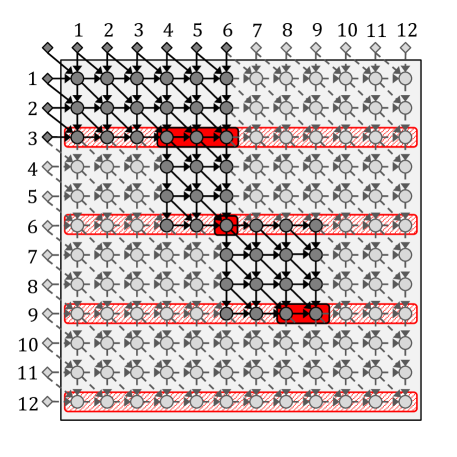
Figure 1: Example square grid and path sketch for $M^{\prime}=3$ and $h=k=4$. The circles are nodes in the square. The diamonds are input nodes (outputs of adjacent squares), omitting irrelevant edges. The red slashes are the 4 superrows, and the solid red are the sketch segments.

The main idea of evaluating the sketch is captured by Figure 1 for the example sketch $\langle 1,4,6\rangle,\langle 2,6,6\rangle,\langle 3,8,9\rangle$. The sketch tells us that shortest paths to $u_{9,8}$ and $u_{9,9}$ pass through one of $u_{3,4},u_{3,5},u_{3,6}$ and the node $u_{6,6}$. Thus, to compute the distances to $u_{9,8}$ and $u_{9,9}$, we need only consider paths through the darker nodes and solid edges—the lighter nodes and dashed edges are not recomputed during evaluation.

The algorithm works as follows. First compute the shortest-path distances to the first segment in the sketch. To do so, horizontally sweep a height-$(M^{\prime}+1)$ column across the $(M^{\prime}+1)\times kM^{\prime}$ slab raising above the $s$-th superrow, keeping two columns in small-memory at a time. Also keep the newly computed distances to the first segment in small-memory, and stop the sweep at the right edge of the segment. More generally, given the distances to a segment in small-memory, we can compute the values for the next segment in the same manner by sweeping a column through the slab. This algorithm yields the following performance.

Lemma 4.

Given a path sketch $\langle s,\ell_{s},r_{s}\rangle,\ldots,\langle i,\ell_{i},r_{i}\rangle$ in an $hM^{\prime}\times kM^{\prime}$ grid with distances to all input nodes computed, our algorithm correctly computes the shortest-path distances to all nodes in the segment $\langle i,\ell_{i},r_{i}\rangle$. Assuming $k\geq h$ and small-memory size $M\geq 5M^{\prime}+\Theta(1)$, the algorithm requires $O(kM^{2})$ operations in small-memory, $O(kM)$ reads, and $0$ writes.

Proof.

Correctness follows from the definition of the path sketch: the sweep performed by the algorithm considers all possible paths that pass through these segments.

The algorithm requires space in small-memory to store two columns in the current slab, the previous segment in the sketch, and the next segment in the sketch, and the two segment boundaries themselves, totaling $4M^{\prime}+\Theta(1)$ small-memory. Due to the monotonically increasing left endpoints of each segment, the horizontal sweep repeats at most $M^{\prime}$ columns per supperrow, so the total number of column iterations is $O(kM^{\prime}+hM^{\prime})=O(kM^{\prime})$. Multiplying by $M^{\prime}$ gives the number of nodes computed.

The main contributor to reads is the input strings themselves to infer the structure/weights of the grid. With $M^{\prime}$ additional small-memory, we can store the “vertical” portion of the input string used while computing each slab, and thus the vertical string is read only once with $O(hM^{\prime})=O(kM^{\prime})$ reads. The “horizontal” input characters can be read with each of the $O(kM^{\prime})$ column-sweep iterations. An additional $k$ reads suffice to read the sketch itself, which is a lower-order term. ∎

Building the path sketch

The main algorithm on each rectangle involves building the set of sketches to segments in the bottom superrow. At some point during the sketch-building process, the distances to each output node is computed, at which point it can be written out. The main idea of the algorithm is a sketch-extension subroutine: given segments in the $i$-th superrow and their sketches, extend the sketches to produce segments in the $(i+1)$-th superrow along with their sketches.

Our algorithm builds up an ordered list of consecutive path sketches, one superrow at a time. The first superrow is partitioned into $k$ segments, each containing exactly $M^{\prime}$ consecutive nodes. The list of sketches is initialized to these segments.

Given a list of sketches to the $i$-th superrow, our algorithm extends the list of sketches to the $(i+1)$-th superrow as follows. The algorithm sweeps a height-$(M^{\prime}+1)$ column across the $(M^{\prime}+1)\times kM^{\prime}$ slab between these superrows (inclusive). The sweep begins at the left end of the slab, reading the input values from the left boundary, and continuing across the entire width of the slab. In small-memory, we evaluate the first segment of the $i$-th superrow (using the algorithm from Lemma 4). Whenever the sweep crosses a segment boundary in the $i$-th superrow, again evaluate the next segment in the $i$-th superrow. For each node in the slab, the sweep calculates both the shortest-path distance and a pointer to the segment in the previous superrow from whence the shortest path originates (or a null pointer if it originates from the left boundary). When the originating segment of the bottom node (the node in the $(i+1)$-th superrow) changes, the algorithm creates a new segment for the $(i+1)$-th superrow and appends it to the sketch of the originating segment. If the segment in the current segment in the $(i+1)$-th superrow grows past $M^{\prime}$ elements, a new segment is created instead and the current path sketch is copied and spliced into the list of sketches. Any sketch that is not extended through this process is no longer relevant and may be spliced out of the list of sketches. When the sweep reaches a node on the output boundary (right edge or bottom edge of the square), the distance to that node is written out.

Lemma 5.

The sketching algorithm partitions the $i$-th superrow into at most $ik$ segments.

Proof.

The proof is by induction over superrows. As a base case, the first superrow consists of exactly $k$ segments. For the inductive step, there are two cases in which a new segment is started in the $(i+1)$-th superrow. The first case is that the originating segment changes, which can occur at most $ik$ times by inductive assumption. The second case is that the current segment grows too large, which can occur at most $k$ times. We thus have at most $(i+1)k$ segments in the $(i+1)$-th superrow. ∎

Lemma 6.

Suppose $h\leq k$ and small-memory $M\geq 11M^{\prime}+\Theta(1)$, and consider an $hM^{\prime}\times kM^{\prime}$ grid with distances to input nodes already computed. Then the sketch building algorithm correctly computes the distances to all output boundary nodes using $O((hk)^{2}M^{2})$ operations in small-memory, $O((hk)^{2}M)$ reads from large-memory, and $O(h^{2}k+X)$ writes to large-memory, where $X=O(kM)$ is the number of boundary nodes written out.

Proof.

Consider the cost of computing each slab, ignoring the writes to the output nodes. We reserve $5M^{\prime}+\Theta(1)$ small-memory for the process of evaluating segments in the previous superrow. To perform the sweep in the current slab, we reserve $M^{\prime}$ small-memory to store one segment in the previous row, $M^{\prime}$ small-memory to store characters in the “vertical” input string, $4(M^{\prime}+1)$ small-memory to store two columns (each with distances and pointers) for the sweep, and an additional $\Theta(1)$ small-memory to keep, e.g., the current segment boundaries. Since there are at most $hk$ segments in the previous superrow (Lemma 5), the algorithm evaluates at most $hk$ segments; applying Lemma 4, the cost is $O(hk^{2}M^{2})$ operations, $O(hk^{2}M)$ reads, and $0$ writes. There are an additional $O(kM^{2})$ operations to sweep through the $kM^{2}$ nodes in the slab, plus $O(kM)$ reads to scan the “horizontal” input string. Finally, there are $O(hk)$ writes to extend existing sketches and $O(hk)$ writes to copy at most $k$ sketches.

Summing across all $h$ slabs and accounting for the output nodes, we get $O((hk)^{2}M^{2}+hkM^{2})$ operations, $O((hk)^{2}M+hkM)$ reads, and $O(h^{2}k+X)$ writes. Removing the lower-order terms gives the lemma. ∎

Combining across all rectangles in the grid, we get the following corollary.

Corollary 1.

Let $m\leq n$ be the length of the two input strings, with $m\geq M$. Suppose $h=O(m/M)$ and $k=O(n/M)$ with $h\leq k$. Then it is possible to compute the LCS or edit distance of the strings with $O(mnhk)$ operations in small-memory, $O(mnhk/M)$ reads to large-memory, and $O(mnh/M^{2}+mn/(hM))$ writes to large-memory.

Proof.

There are $\Theta(mn/(hkM^{2}))$ size-$(hM/11)\times(kM/11)$ subgrids. Multiplying by the cost of each grid (Lemma 6) gives the bound. ∎

Setting $h=k=1$ gives the standard $M\times M$ tiling with $O(nm)$ time and $O(mn\omega/M)$ ARAM cost. As the size of squares increase, the fraction of output nodes and hence writes decreases, at the cost of more overhead for operations in small-memory and reads from large-memory. Assuming both $n$ and $m$ are large enough to do so, plugging in $h=k=\max\{1,k_{T}\}$ or $h=k=k_{Q}$ with a few steps of algebra to eliminate terms yields Theorem 4.

6 Single-Source Shortest Paths

The single-source shortest-paths (SSSP) problem takes a directed weighted graph $G=(V,E)$ and a source vertex $s\in V$, and outputs the shortest distances $d(s,v)$ from $s$ to every other vertex in $v\in V$. For graphs with non-negative edge weights, the most efficient algorithm is Dijkstra’s algorithm [18].

In this section we will study (variants of) Dijkstra’s algorithm in the asymmetric setting. We describe and analyze three versions (two classical and one new variant) of Dijkstra’s algorithm, and the best version can be chosen based on the values of $M$, $\omega$, the number of vertices $n=|V|$, and the number of edges $m=|E|$.

Theorem 5.

The SSSP problem on a graph $G=(V,E)$ with non-negative edge weights can be solved with $\displaystyle Q(n,m)=O\mathopen{}\mathclose{{}\left(\min\mathopen{}\mathclose{{}\left(n\mathopen{}\mathclose{{}\left(\omega+\frac{m}{M}}\right),\omega(m+n\log n),m(\omega+\log n)}\right)}\right)$ and $T(n,m)=O(Q(n,m)+n\log n)$, both in expectation, on the $(M,\omega)$-ARAM.

We start with the classical Dijkstra’s algorithm [18], which maintains for each vertex $v$, $\delta(v)$, a tentative upper bound on the distance, initialized to $+\infty$ (except for $\delta(s)$, which is initialized to $0$). The algorithm consists of $n-1$ iterations, and the final distances from $s$ are stored in $\delta(\cdot)$. In each iteration, the algorithm selects the unvisited vertex $u$ with smallest finite $\delta(u)$, marks it as visited, and uses its outgoing edges to relax (update) all of its neighbors’ distances. A priority queue is required to efficiently select the unvisited vertex with minimum distance. Using a Fibonacci heap [24], the time of the algorithm is $O(m+n\log n)$ in the standard (symmetric) RAM model. In the $(M,\omega)$-ARAM, the costs are $Q=T=O((m+n\log n)\omega)$ since the Fibonacci heap requires asymptotically as many writes as reads. Alternatively, using a binary search tree for the priority queue reduces the number of writes (see Section 4) at the cost of increasing the number of reads, giving $Q=T=$ $O(m\log n+\omega{}m)$. These bounds are better when $m=o(\omega{}n)$. Both of these variants store the priority queue in large-memory, requiring at least one write to large-memory per edge.

We now describe an algorithm, which we refer to as phased Dijkstra, that fully maintains the priority queue in small-memory and only requires $O(n)$ writes to large-memory. The idea is to partition the computation into phases such that for a parameter $M^{\prime}$ each phase needs a priority queue of size at most $2M^{\prime}$ and visits at least $M^{\prime}$ vertices. By selecting $M^{\prime}=M/c$ for an appropriate constant $c$, the priority queue fits in small-memory, and the only writes to large-memory are the final distances.

Each phase starts and ends with an empty priority queue $P$ and consists of two parts. A Fibonacci heap is used for $P$, but is kept small by discarding the $M^{\prime}$ largest elements (vertex distances) whenever $|P|=2M^{\prime}$. To do this $P$ is flattened into an array, the $M^{\prime}$-th smallest element $d_{\mbox{\scriptsize\emph{max}}}$ is found by selection, and the Fibonacci heap is reconstructed from the elements no greater than $d_{\mbox{\scriptsize\emph{max}}}$, all taking linear time. All further insertions in a given phase are not added to $P$ if they have a value greater than $d_{\mbox{\scriptsize\emph{max}}}$. The first part of each phase loops over all edges in the graph and relaxes any that go from a visited to an unvisited vertex (possibly inserting or decreasing a key in $P$). The second part then runs the standard Dijkstra’s algorithm, repeatedly visiting the vertex with minimum distance and relaxing its neighbors until $P$ is empty. To implement relax, the algorithm needs to know whether a vertex is already in $P$, and if so its location in $P$ so that it can do a decrease-key on it. It is too costly to store this information with the vertex in large-memory, but it can be stored in small-memory using a hash table.

The correctness of this phased Dijkstra’s algorithm follows from the fact that it only ever visits the closest unvisited vertex, as with the standard Dijkstra’s algorithm.

Lemma 7.

Phased Dijkstra’s has $\displaystyle Q(n,m)=O\mathopen{}\mathclose{{}\left(n\mathopen{}\mathclose{{}\left(\omega+\frac{m}{M}}\right)}\right)$ and $T(n,m)=O(Q(n,m)+n\log n)$ both in expectation (for $M\leq n$).

Proof.

During a phase either the size of $P$ will grow to $2M^{\prime}$ (and hence delete some entries) or it will finish the algorithm. If $P$ grows to $2M^{\prime}$ then at least $M^{\prime}$ vertices are visited during the phase since that many need to be deleted with delete-min to empty $P$. Therefore the number of phases is at most $\lceil n/M^{\prime}\rceil$. Visiting all edges in the first part of each phase involves at most $m$ insertions and decrease-keys into $P$, each taking $O(1)$ amortized time in small-memory, and $O(1)$ time to read the edge from large-memory. Since compacting $Q$ when it overflows takes linear time, its cost can be amortized against the insertions that caused the overflow. The cost across all phases for the first part is therefore $Q=W=O(m\lceil n/M^{\prime}\rceil)$. For the second part, every vertex is visited once and every edge relaxed at most once across all phases. Visiting a vertex requires a delete-min in small-memory and a write to large-memory, while relaxing an edge requires an insert or decrease-key in small-memory, and $O(1)$ reads from large-memory. We therefore have for this second part (across all phases) that $Q=O(\omega n+m)$ and $W=O(n(\omega+\log n)+m)$. The operations on $P$ each include an expected $O(1)$ cost for the hash table operations. Together this gives our bounds. ∎

Compared to the first two versions of Dijkstra’s algorithm with $Q=T=O(\omega{}m+\min(\omega{}n\log n,m\log n))$, the new algorithm is strictly better when $\omega M>n$. More specifically, the new algorithm performs better when $nm/M<\max\{\omega{}m,\min(\omega{}n\log n,m\log n)\}$. Combining these three algorithms proves Theorem 5, when the best one is chosen based on the parameters $M$, $\omega$, $n$, and $m$.

7 Minimum Spanning Tree (MST)

In this section we discuss several commonly-used algorithms for computing a minimum spanning tree (MST) on a weighted graph $G=(V,E)$ with $n=|V|$ vertices and $m=|E|$ edges. Some of them are optimal in terms of the number of writes ($O(n)$). Although loading a graph into large-memory requires $O(m)$ writes, the algorithms are still useful on applications that compute multiple MSTs based on one input graph. For example, it can be useful for computing MSTs on subgraphs, such as road maps, or when edge weights are time-varying functions and hence the graph maintains its structure but the MST varies over time.

Prim’s algorithm. All three versions of Dijkstra’s algorithm discussed in Section 6 can be adapted to implement Prim’s algorithm [16]. Thus, the upper bounds of ARAM cost and time in Theorem 5 also hold for minimum spanning trees.

Kruskal’s algorithm. The initial sorting phase requires $Q=T=O(m\log n+\omega{}m)$ [9]. The second phase constructs a MST using union-find without path compression in $O(m\log n)$ time, and performs $O(n)$ writes (the actual edges of the MST). Thus, the complexity is dominated by the first phase. Neither ARAM cost nor time match our variant of Borůvka’s algorithm.

Borůvka’s algorithm. Borůvka’s algorithm consists of at most $\log n$ rounds. Initially all vertices belong in their own component, and in each round, the lightest edges that connect each component to another component are added to the edge set of the MST, and components are merged using these edges. This merging can be done using, for example, depth first search among the components and hence takes time proportional to the number of remaining components. However, since edges are between original vertices the algorithm is required to maintain a mapping from vertices to the component they belong to. Shortcutting all vertices on each round to point directly to their component requires $O(n)$ writes per round and hence up to $O(n\log n)$ total writes across the rounds. This is not a bottleneck in the standard RAM model but is in the asymmetric case.

We now describe a variant of Borůvka’s algorithm which is asymptotically optimal in the number of writes. It requires only $O(1)$ small-memory. The algorithm proceeds in two phases. For the first $\log\log n$ rounds, the algorithm performs no shortcuts (beyond the merging of components). Thus it will leave chains of length up to $\log\log n$ that need to be followed to map each vertex to the component it belongs to. Since there are at most $O(m\log\log n)$ queries during the first $\log\log n$ rounds and each only require reads, the total time for identifying the minimum edges between components in the first phase is $O(m(\log\log n)^{2})$. After the first phase all vertices are shortcut to point to their component. We refer to these components as the phase-one components. In the second phase, on every round, we shortcut the phase-one components to point directly to the component they belong to. Since there can only be at most $n/\log n$ phase-one components, and at most $\log n-\log\log n$ rounds in phase-two, the total number of reads and writes for these updates is $O(n)$. During phase two the mapping from a vertex to its component takes two steps: one to find its phase-one component and another to get to the current component. Therefore the total time for identifying the minimum edges between components in the second phase is $O(m\log n)$.

All other work is on the components themselves (i.e. adding the forest of minimum edges and performing DFS to merge components). The number of reads, writes, and other instructions is proportional to the number of components. There are $n$ components on the first round and the number decreases by at least a factor of two on each following round. Therefore the total time on the components is $O(\omega n)$. Summing the costs give the following lemma.

Lemma 8.

Our variant of Borůvka’s algorithm generates a minimum spanning tree on a graph with $n$ vertices and $m$ edges with ARAM cost and time $Q(n,m)=T(n,m)=O(m\log n+\omega{}n)$ on the $(M,\omega)$-ARAM.

Theorem 6.

A minimum spanning tree on a graph $G=(V,E)$ can be computed with ARAM cost $\displaystyle Q(n,m)=O\mathopen{}\mathclose{{}\left(m\min\mathopen{}\mathclose{{}\left({n\over M},\log n}\right)+\omega n}\right)$ and time $T(n,m)=O(Q(n,m)+n\log n)$ on the $(M,\omega)$-ARAM.

The theorem is a combination of the bounds of Prim’s and Borůvka’s algorithms (the $n/M$ term is in expectation).

Acknowledgments

This research was supported in part by NSF grants CCF-1314590, CCF-1314633 and CCF-1533858, the Intel Science and Technology Center for Cloud Computing, and the Miller Institute for Basic Research in Science at UC Berkeley.

Appendix A Longest Common Subsequence: Further Results

• Let $k_{T}=\min\{(\omega{}/M)^{1/3},\sqrt{M}\}$ and suppose $m,n=\Omega(k_{T}M)$. Then it is possible to compute the length of the LCS or edit distance with total time $T(m,n)=O(mn+mn\omega/(Mk_{T}))$.

  Let $k_{Q}=\min\{\omega^{1/3},\sqrt{M}\}$ and suppose $m,n=\Omega(k_{Q}M)$. Then it is possible to compute the length of the LCS or edit distance with an ARAM cost of $Q(m,n)=O(mn\omega/(k_{Q}M))$.

Proof.

As long as $h\leq\sqrt{M}$, the number of writes reduces to $O(mn/(hM))$. (Increasing $h$ further causes the number of writes to increase.)

Consider the time bound first. If $k_{T}\leq 1$, then just use algorithm with $h=k=1$. Otherwise, let $M^{\prime}=M/11$ and use the algorithm with $h=k=k_{T}$. As long as $h=k\leq(\omega/M)^{1/3}$, which is true for $k_{T}$, the time of operations is less than the time of writes, giving the bound.

For the ARAM cost, use our algorithm with $h=k=k_{Q}$. As long as $h=k\leq\omega^{1/3}$, then cost of reads is less than the cost of writes. ∎

Improving the bound for smaller string lengths. If $m\leq M$, then the standard I/O algorithm becomes even better — simply sweep a column through, which remains in small-memory, using $O(m+n)$ reads, no writes, and $O(mn)$ time. Since there are no writes, we cannot beat that bound. As described already, if $m\geq kM^{\prime}$ then our algorithm partitions the grid into $kM^{\prime}\times kM^{\prime}$ squares, which for larger $k$ saves writes by sacrificing reads and re-computation. The remaining question is what happens when $m$ is larger than small-memory but not too much larger, i.e., $M<m<k_{T}M^{\prime}$ or $M<m<k_{Q}M^{\prime}$.

When $m$ falls in this range, we apply the algorithm to $m\times kM^{\prime}$ rectangles, i.e., setting $h=m/M^{\prime}$. It turns out we can achieve a better bound than Theorem 4 by increasing $k$ even further. The key observation here is that the bottom of the rectangle no longer needs to be written out because there is no rectangle below it — only the right edge is an output edge. The number of writes per rectangle (Lemma 6 with $X=hM^{\prime}$) reduces to $O(h^{2}k+hM)$. We thus have the following modified version of Corollary 1

Corollary 2.

Let $m\leq n$ be the length of the two input strings, with $m\geq M$. Let $h=\Theta(m/M)$, and suppose $k=O(n/M)$ satisfying $h\leq k$. Then it is possible to compute LCS or edit distance of a length $m$ and $n$ input strings with $O(mnhk)$ operations in small-memory, $O(mnhk/M)$ reads to large-memory, and $O(mnh/M^{2}+mn/(kM))$ writes to large-memory.

Proof.

There are $\Theta(n/(kM))$ size $m\times(kM/11)$ subgrids. Multiplying by the cost of each grid from Lemma 6, with $X=hM$, gives $O(nh^{2}kM)$ operations, $O(nh^{2}k)$ reads, and $O(nh^{2}/M+nh/k)$ writes. Substituting one of the $h$ terms with $h=\Theta(m/M)$ gives the theorem. ∎

The following theorem provides the improved time and ARAM cost in the case that one string is short but the other is long. To understand the bounds here, consider the maximum and minimum values of $h$ for $h=m/M^{\prime}$ and large $\omega$. If $h=(\omega/M)^{1/3}$, i.e., $m$ is large enough that we can divide into $k_{T}M^{\prime}\times k_{T}M^{\prime}$ squares, then we get $k_{T}^{\prime}=(\omega/M)^{1/3}$ matching the bound in Theorem 4. As $h$ decreases, the bound improves. In the limit, $h=\Theta(1)$ (or $m=\Theta(M)$), we get $k_{T}^{\prime}=\sqrt{\omega/M}$ which is better.

Theorem 7.

Let $h=\Theta(m/M)$ and suppose that $h\leq k_{T}$ specified in Theorem 4. Let $k_{T}^{\prime}=\min\{\sqrt{\omega/(hM)},M/h\}$ and suppose that $n=\Omega(k_{T}^{\prime}M)$. Then it is possible to compute the length of the LCS or edit distance with total time of $T(m,n)=O(mn+mn\omega/(k_{T}^{\prime}M))$.

Let $h=\Theta(m/M)$ and suppose that $h\leq k_{Q}$ specified in Theorem 4. Let $k_{Q}^{\prime}=\min\{\sqrt{\omega/h},M/h\}$ and suppose $n=\Omega(k_{Q}^{\prime}M)$. Then it is possible to compute the length of the LCS or edit distance with an ARAM cost of $Q(m,n)=O(mn\omega/(k_{Q}^{\prime}M))$.

Proof.

With the restrictions on $h$, we have $h\leq k$, so Corollary 2 is applicable. As in proof of Theorem 4, the second term of the min has the effect that $O(mnh/M^{2}+mn/(kM))=O(mn/(kM))$. The rest of the bound follows by choice of $k$ to makes the cost of writes dominate. ∎

When $n$ is also small, the bound improves further. In this case, the algorithm consists of building the sketch on a single $m\times n$ grid, so no boundary nodes are output — the only writes that need be performed are the sketch itself.

Theorem 8.

Let $m\leq n$ be the length of the two input strings, with $m\geq M$. Let $h=\Theta(m/M)$ and let $k=\Theta(n/M)$. Then it is possible to compute the LCS or edit distance of the two strings with time $T(m,n)=O(mnhk+h^{2}k\omega)$ and ARAM cost $Q(m,n)=O(mnhk/M+h^{2}k\omega)$.

Proof.

The bound follows directly from Lemma 6 with $X=0$ and substituting one $hk$ term in the read/time bounds. ∎

Recovering the shortest path. The standard approach for outputting the shortest path is to trace backwards through the grid from the bottom-rightmost node. This approach assumes that the distances to all internal nodes are known, but unfortunately our algorithm discards distances to interior nodes.

Fortunately, the sketch provides enough information to cheaply traceback a path through each square without any additional writes (except the path itself) and without asymptotically more reads or time. In particular, for any node $v$ in superrow $i+1$, it is not hard to identify a node $u$ in superrow $i$ such that a shortest path to $v$ passes through $u$. Consider the sketch $\langle s,\ell_{s},r_{s}\rangle,\ldots,\langle i,\ell_{i},r_{i}\rangle,\langle i+1,\ell_{i+1},r_{i+1}\rangle$ to the segment $\langle i+1,\ell_{i+1},r_{i+1}\rangle$ that includes $v$. The vertex $u$ is one of the vertices in the penultimate segment $\langle i,\ell_{i},r_{i}\rangle$ of the sketch, so the goal is to identify which one. To do so, evaluate the sketch to the segment $\langle i,\ell_{i},r_{i}\rangle$. Then perform a horizontal sweep through the final slab, keeping track of the originating vertex from the penultimate segment.

Now suppose we have these vertices $u$ and $v$ that fall along the shortest path and are in consecutive superrows. We also need to identify the path through the slab between $u$ and $v$. To do that, we apply Hirschberg’s [27] recursive low-space algorithm for path recovery in the ED/LCS grid, splitting the horizontal dimension in half on each recursion. Note that the time reduces by a constant fraction in each recursion, but the ARAM cost does not (the only ARAM cost here is from reading the “horizontal” input string), so it may not be immediately obvious that the ARAM cost is cheap enough. Fortunately, after recursing at most $\lg k$ times, the length of the horizontal substring is at most $M^{\prime}$ and the remaining path-recovery subproblem can be done with no further reads from large-memory.

Putting it all together, tracing a path to the previous superrow requires one sketch evaluation, followed by time that is linear in the area and an ARAM cost that corresponds to reading the horizontal string from large-memory $\lg k$ times. Rounding up loosely, we get time of $O(k(M^{\prime})^{2}+(M)(kM))=O(kM^{2})$ along with $O(kM^{\prime}+(kM^{\prime})\lg k)=O(k^{2}M)$ reads. Multiplying by the $h$ superrows, we have $O(hkM^{2})$ time and $O(hk^{2}M)$ reads from large-memory. Both of these are less than the cost of building the sketch in the first place (Lemma 6).

Appendix B Write-Efficient Floyd–Warshall Algorithm

The Floyd–Warshall algorithm solves the all-pairs shortest path problem on weighted graphs [23]. It requires $O(n^{3})$ writes in its original and currently recognized form and hence $O(\omega n^{3})$ time in $(M,\omega)$-ARAM. Here we describe how to reorganize the computation so that it only requires $T=O(n^{3}+\omega{}n^{2})$ time. Compared to the version described in Section 4, this algorithm is easier to program, and has a smaller constant coefficient.

Consider a graph $G$ with vertices $V=\{1,\ldots,n\}$ and a function $\mbox{ShortestPath}(i,j,k)$ that returns the shortest possible path from $i$ to $j$ using vertices only from the set $\{1,2,\ldots,k\}$ as intermediate points along the path. $\mbox{ShortestPath}(i,j,k)$ can be computed using the Floyd–Warshall algorithm with the following update rule:

$$\mbox{ShortestPath}(i,j,k)=\min\{\mbox{ShortestPath}(i,j,k-1),\mbox{ShortestPath}(i,k,k-1)+\mbox{ShortestPath}(k,j,k-1)\}$$

where $\mbox{ShortestPath}(i,j,0)$ is initialized as the weight of the edge from vertex $i$ to vertex $j$ ($+\infty$ if the edge does not exist). The shortest path from vertex $i$ to vertex $j$ is stored in $\mbox{ShortestPath}(i,j,n)$, after the computation is finished.

With this formulation of the DP, $O(n^{3})$ writes will be required. We now introduce an alternative and equivalent formulation of the DP that will reduce the number of writes to $O(n^{2})$. Let $A(i,k)$ be $\mbox{ShortestPath}(i,k,k-1)$ and $B(k,j)$ be $\mbox{ShortestPath}(k,j,k-1)$ (with the same initialization as before for $A(i,1)$ and $B(1,i)$). Then they can be computed as:

$$A(i,k)=\min_{k^{\prime}<k}\{A(i,k^{\prime})+B(k^{\prime},k)\}$$

$$B(k,j)=\min_{k^{\prime}<k}\{A(k,k^{\prime})+B(k^{\prime},j)\}$$

in increasing order of $k$ from $1$ to $n$. After $A(i,k)$ and $B(k,j)$ are calculated, the shortest distance $D(i,j)$ from vertex $i$ to vertex $j$ (equivalent to $\mbox{ShortestPath}(i,j,n)$) can be computed as:

$$D(i,j)=\min_{1\leq k\leq n}\{A(i,k)+B(k,j)\}$$

Clearly the computation of the new DP requires only $O(n^{2})$ writes. The correctness can be easily shown by verifying that $D(i,j)$ is equivalent to $\mbox{ShortestPath}(i,j,n)$.

References

- [1] Alok Aggarwal and Jeffrey S. Vitter. The Input/Output complexity of sorting and related problems. Communications of the ACM, 31(9), 1988.
- [2] Alfred V. Aho, John E. Hopcroft, and Jeffrey D. Ullman. The Design and Analysis of Computer Algorithms. Addison-Wesley, Reading, MA, 1974.
- [3] Miklós Ajtai, János Komlós, and Endre Szemerédi. An sorting network. In Proc. ACM Symposium on Theory of Computing (STOC), 1983.
- [4] Deepak Ajwani, Andreas Beckmann, Riko Jacob, Ulrich Meyer, and Gabriel Moruz. On computational models for flash memory devices. In Proc. ACM International Symposium on Experimental Algorithms (SEA), 2009.
- [5] Ameen Akel, Adrian M. Caulfield, Todor I. Mollov, Rajech K. Gupta, and Steven Swanson. Onyx: A prototype phase change memory storage array. In Proc. USENIX Workshop on Hot Topics in Storage and File Systems (HotStorage), 2011.
- [6] Manos Athanassoulis, Bishwaranjan Bhattacharjee, Mustafa Canim, and Kenneth A. Ross. Path processing using solid state storage. In Proc. International Workshop on Accelerating Data Management Systems Using Modern Processor and Storage Architectures (ADMS), 2012.
- [7] Avraham Ben-Aroya and Sivan Toledo. Competitive analysis of flash-memory algorithms. In Proc. European Symposium on Algorithms (ESA), 2006.
- [8] Naama Ben-David, Guy E. Blelloch, Jeremy T. Fineman, Phillip B. Gibbons, Yan Gu, Charlie McGuffey, and Julian Shun. Parallel algorithms for asymmetric read-write costs. In Proc. ACM Symposium on Parallelism in Algorithms and Architectures (SPAA), 2016.
- [9] Guy E. Blelloch, Jeremy T. Fineman, Phillip B. Gibbons, Yan Gu, and Julian Shun. Sorting with asymmetric read and write costs. In Proc. ACM Symposium on Parallelism in Algorithms and Architectures (SPAA), 2015.
- [10] Erin Carson, James Demmel, Laura Grigori, Nicholas Knight, Penporn Koanantakool, Oded Schwartz, and Harsha V. Simhadri. Write-avoiding algorithms. In Proc. IEEE International Parallel & Distributed Processing Symposium (IPDPS), 2016.
- [11] Shimin Chen, Phillip B. Gibbons, and Suman Nath. Rethinking database algorithms for phase change memory. In Proc. Conference on Innovative Data Systems Research (CIDR), 2011.
- [12] Shimin Chen and Qin Jin. Persistent B+-trees in non-volatile main memory. PVLDB, 8(7), 2015.
- [13] Sangyeun Cho and Hyunjin Lee. Flip-N-Write: A simple deterministic technique to improve PRAM write performance, energy and endurance. In Proc. IEEE/ACM International Symposium on Microarchitecture (MICRO), 2009.
- [14] Rezaul A. Chowdhury and Vijaya Ramachandran. Cache-oblivious dynamic programming. In Proc. ACM-SIAM Symposium on Discrete Algorithms (SODA), 2006.
- [15] Stephen Cook and Ravi Sethi. Storage requirements for deterministic polynomial time recognizable languages. Journal of Computer and System Sciences, 13(1), 1976.
- [16] Thomas H. Cormen, Charles E. Leiserson, Ronald L. Rivest, and Clifford Stein. Introduction to Algorithms (3rd edition). MIT Press, 2009.
- [17] Mark de Berg, Otfried Cheong, Mark van Kreveld, and Mark Overmars. Computational Geometry: Algorithms and Applications. Springer-Verlag, 2008.
- [18] Edsger W. Dijkstra. A note on two problems in connexion with graphs. Numerische mathematik, 1(1), 1959.
- [19] Xiangyu Dong, Norman P. Jouupi, and Yuan Xie. PCRAMsim: System-level performance, energy, and area modeling for phase-change RAM. In Proc. ACM International Conference on Computer-Aided Design (ICCAD), 2009.
- [20] Xiangyu Dong, Xiaoxia Wu, Guangyu Sun, Yuan Xie, Hai H. Li, and Yiran Chen. Circuit and microarchitecture evaluation of 3D stacking magnetic RAM (MRAM) as a universal memory replacement. In Proc. ACM Design Automation Conference (DAC), 2008.
- [21] David Eppstein, Michael T. Goodrich, Michael Mitzenmacher, and Pawel Pszona. Wear minimization for cuckoo hashing: How not to throw a lot of eggs into one basket. In Proc. ACM International Symposium on Experimental Algorithms (SEA), 2014.
- [22] Jittat Fakcharoenphol and Satish Rao. Planar graphs, negative weight edges, shortest paths, near linear time. In Proc. IEEE Symposium on Foundations of Computer Science (FOCS), 2001.
- [23] Robert W. Floyd. Algorithm 97: Shortest path. Commun. ACM, 5(6):345–, June 1962.
- [24] Michael L. Fredman and Robert E. Tarjan. Fibonacci heaps and their uses in improved network optimization algorithms. Journal of the ACM, 34(3), 1987.
- [25] Eran Gal and Sivan Toledo. Algorithms and data structures for flash memories. ACM Computing Surveys, 37(2), 2005.
- [26] Michael T. Goodrich. Zig-zag sort: A simple deterministic data-oblivious sorting algorithm running in time. In Proc. ACM Symposium on Theory of Computing (STOC), 2014.
- [27] D. S. Hirschberg. A linear space algorithm for computing maximal common subsequences. Commun. ACM, 18(6):341–343, June 1975.
- [28] Jia-Wei Hong and H. T. Kung. I/O complexity: The red-blue pebble game. In Proc. ACM Symposium on Theory of Computing (STOC), 1981.
- [29] John Hopcroft, Wolfgang Paul, and Leslie Valiant. On time versus space. Journal of the ACM, 24(2), 1977.
- [30] HP, SanDisk partner on memristor, ReRAM technology. http://www.bit-tech.net/news/ hardware/2015/10/09/hp-sandisk-reram-memristor, October 2015.
- [31] Jingtong Hu, Qingfeng Zhuge, Chun Jason Xue, Wei-Che Tseng, Shouzhen Gu, and Edwin Sha. Scheduling to optimize cache utilization for non-volatile main memories. IEEE Transactions on Computers, 63(8), 2014.
- [32] www.slideshare.net/IBMZRL/theseus-pss-nvmw2014, 2014.
- [33] Intel and Micron produce breakthrough memory technology. http://newsroom.intel.com/ community/intel_newsroom/blog/2015/07/28/intel-and-micron-produce-breakthrough-memory-technology, July 2015.
- [34] Hyojun Kim, Sangeetha Seshadri, Clement L. Dickey, and Lawrence Chu. Evaluating phase change memory for enterprise storage systems: A study of caching and tiering approaches. In Proc. USENIX Conference on File and Storage Technologies (FAST), 2014.
- [35] Philip N. Klein, Shay Mozes, and Oren Weimann. Shortest paths in directed planar graphs with negative lengths: A linear-space -time algorithm. ACM Transactions on Algorithms, 6(2), 2010.
- [36] Benjamin C. Lee, Engin Ipek, Onur Mutlu, and Doug Burger. Architecting phase change memory as a scalable DRAM alternative. In Proc. ACM International Symposium on Computer Architecture (ISCA), 2009.
- [37] Jagan S. Meena, Simon M. Sze, Umesh Chand, and Tseung-Yuan Tseng. Overview of emerging nonvolatile memory technologies. Nanoscale Research Letters, 9, 2014.
- [38] Suman Nath and Phillip B. Gibbons. Online maintenance of very large random samples on flash storage. VLDB J., 19(1), 2010.
- [39] Hyoungmin Park and Kyuseok Shim. FAST: Flash-aware external sorting for mobile database systems. Journal of Systems and Software, 82(8), 2009.
- [40] Joon-Sang Park, Michael Penner, and Viktor K. Prasanna. Optimizing graph algorithms for improved cache performance. IEEE Transactions on Parallel and Distributed Systems, 15(9), 2004.
- [41] Mike S. Paterson. Improved sorting networks with depth. Algorithmica, 5(1), 1990.
- [42] Moinuddin K. Qureshi, Sudhanva Gurumurthi, and Bipin Rajendran. Phase Change Memory: From Devices to Systems. Morgan & Claypool, 2011.
- [43] Jeanette P. Schmidt. All shortest paths in weighted grid graphs and its application to finding all approximate repeats in strings. SIAM Journal on Computing, 27, 1998.
- [44] Joel Seiferas. Sorting networks of logarithmic depth, further simplified. Algorithmica, 53(3), 2009.
- [45] Robert E. Tarjan. Updating a balanced search tree in rotations. Information Processing Letters, 16(5), 1983.
- [46] Stratis D. Viglas. Adapting the B+-tree for asymmetric I/O. In Proc. East European Conference on Advances in Databases and Information Systems (ADBIS), 2012.
- [47] Stratis D. Viglas. Write-limited sorts and joins for persistent memory. PVLDB, 7(5), 2014.
- [48] Cong Xu, Xiangyu Dong, Norman P. Jouppi, and Yuan Xie. Design implications of memristor-based RRAM cross-point structures. In Proc. IEEE Design, Automation and Test in Europe (DATE), 2011.
- [49] Byung-Do Yang, Jae-Eun Lee, Jang-Su Kim, Junghyun Cho, Seung-Yun Lee, and Byoung-Gon Yu. A low power phase-change random access memory using a data-comparison write scheme. In Proc. IEEE International Symposium on Circuits and Systems (ISCAS), 2007.
- [50] Yole Developpement. Emerging non-volatile memory technologies, 2013.
- [51] Ping Zhou, Bo Zhao, Jun Yang, and Youtao Zhang. A durable and energy efficient main memory using phase change memory technology. In Proc. ACM International Symposium on Computer Architecture (ISCA), 2009.
- [52] Omer Zilberberg, Shlomo Weiss, and Sivan Toledo. Phase-change memory: An architectural perspective. ACM Computing Surveys, 45(3), 2013.