Exact diatomic Fermi-Pasta-Ulam-Tsingou solitary waves with optical band ripples at infinity

Abstract.

We study the existence of solitary waves in a diatomic Fermi-Pasta-Ulam-Tsingou (FPUT) lattice. For monatomic FPUT the traveling wave equations are a regular perturbation of the Korteweg-de Vries (KdV) equation’s but, surprisingly, we find that for the diatomic lattice the traveling wave equations are a singular perturbation of KdV’s. Using a method first developed by Beale to study traveling solutions for capillary-gravity waves we demonstrate that for wave speeds in slight excess of the lattice’s speed of sound there exists nontrivial traveling wave solutions which are the superposition an exponentially localized solitary wave and a periodic wave whose amplitude is extremely small. That is to say, we construct nanopteron solutions. The presence of the periodic wave is an essential part of the analysis and is connected to the fact that linear diatomic lattices have optical band waves with any possible phase speed.

We consider the problem of traveling waves in a diatomic Fermi-Pasta-Ulam-Tsingou (FPUT) lattice. The physical situation is this: suppose that infinitely many particles are arranged on a line. The mass of the $j$th (where $j\in{\bf{Z}}$) particle is

$$m_{j}=\begin{cases}m_{1}&\text{ when $j$ is odd}\\ m_{2}&\text{when $j$ is even.}\end{cases}$$

Without loss of generality we assume that $m_{1}>m_{2}>0$. The position of the $j$th particle at time $\bar{t}$ is $\bar{y}_{j}(\bar{t})$. Suppose that each mass is connected to its two nearest neighbors by a spring and furthermore assume that each spring is identical to every other spring in the sense that the force exerted by said spring when stretched by an amount $r$ from its equilibrium length $l_{s}$ is given by

$$F_{s}(r):=-k_{s}r-b_{s}r^{2}$$

where $k_{s}>0$ and $b_{s}\neq 0$ are specified constants. Such a system is called a “diatomic lattice” or “dimer.” Newton’s law gives the equations of motion for the system:

(0.1) $$m_{j}{d^{2}\bar{y}_{j}\over d\bar{t}^{2}}=-k_{s}\bar{s}_{j-1}-b_{s}\bar{s}_{j-1}+k_{s}\bar{s}_{j}+b_{s}\bar{s}^{2}_{j}$$

where $\bar{s}_{j}:=\bar{y}_{j+1}-\bar{y}_{j}-l_{s}.$

In the setting where $m_{1}=m_{2}$ it is well-known that there exist localized traveling wave solutions of (0.1), see the seminal articles of Friesecke & Wattis [FW94] and Friesecke & Pego [FP99]. Here we are interested in extending this result to the diatomic case where $m_{1}>m_{2}$. There has been quite a bit of interest in the propagation of waves through polyatomic FPUT lattices. Such systems represent a paradigm for the evolution of waves through heterogeneous and nonlinear granular media (see [Bri53] and [Kev11] for an overview). There are several existence proofs for traveling spatially periodic waves for polyatomic problems [BP13] [Qin15], a number of semi-rigourous asymptotics for solitary wave solutions in various contexts [JSVG13], as well as both formal and rigorous results which state that polyatomic FPUT with periodic material coefficients is well-approximated by the soliton bearing Korteweg-de Vries (KdV) equation over very long time scales [PFR86] [CBCPS12] [GMWZ14]. While all of this previous work strongly suggests that localized traveling waves for polyatomic FPUT will exist, the question of whether a truly localized traveling wave akin to those developed in [FP99] remains open. In this article we demonstrate that the answer to this question—at least for waves which travel at a speed just a bit larger than the speed of sound—is “sort of.”

As it happens, the existence problem is inescapably singular. This is particularly surprising because the existence proof of small amplitude solitary waves for monatomic FPUT in [FP99] goes through using regular perturbation methods. In that article, the equation for the solitary wave’s profile $\phi$ is shown to be equivalent to $\phi=p_{c}(\phi^{2})$ where $p_{c}$ is a Fourier multiplier operator and $c$ is the speed of propagation. Making the “long wave scaling” $\phi(x)=\epsilon^{2}\Phi(\epsilon x)$ and $c=c_{sound}+\epsilon^{2}$ yields $\Phi=P_{\epsilon}(\Phi^{2})$. The hinge on which their result turns is the fact that the operator $P_{\epsilon}$ converges in the operator norm to $(1-\partial_{X}^{2})^{-1}$ as $\epsilon\to 0^{+}$. Which means that the traveling wave equation at $\epsilon=0$ can be rewritten as $\Phi^{\prime\prime}-\Phi+\Phi^{2}=0$. This is the traveling wave equation for KdV and has $\operatorname{sech}^{2}$ type solutions. Moreover, using classical results from quantum mechanics, they show that the linearization of the equation $\Phi=P_{0}(\Phi^{2})$ at the KdV solitary wave results in an operator which is invertible on even functions. This, with the uniform convergence of $P_{\epsilon}$, allows them to extend the wave’s existence to $\epsilon>0$ using a quantitative inverse function theorem.

This process goes awry in the diatomic setting. In this case the dispersion relation for the linearization of (0.1) has two parts. The “acoustic” band, which is more or less just like the dispersion relation for the monatomic problem, and the “optical” band which does not exist in the monatomic problem at all. Roughly speaking, we are able to decompose our problem into a pair of equations, one for the acoustic part and another for the optical part. The analysis for the acoustic part goes forward along lines much like in the monatomic case of [FP99]; it limits to a KdV traveling wave equation. On the other hand, the equation for the optical part is classically singularly perturbed in the sense that the highest derivative of the unknown is multiplied by the small parameter $\epsilon$.

The possible outcomes for singularly perturbed problems like this is pretty vast, of course. Many of the approaches for sussing out the consequences are either geometric or dynamical in nature. Our problem is nonlocal and as such it is not obvious to us how to use, say, geometric singular perturbation theory (as in [AGJ90] for instance) or fast-slow averaging (e.g. [BYB10]) to our setting. And so we turn to the functional analytic approach developed by Beale to prove the existence of solitary capillary-gravity waves in his staggering article [Bea91].

Here is what we discover:

Theorem 1.

Suppose that $m_{1}>m_{2}>0$. For wavespeeds $c$ sufficiently close to, but larger than, the speed of sound of the lattice, $c_{sound}:=\sqrt{2k_{s}/(m_{1}+m_{2})}$, there exist traveling wave solutions of the diatomic FPUT problem which are the superposition of two pieces. One piece is a nonzero exponentially localized function that is a small perturbation of a $\operatorname{sech}^{2}$ profile which, in turn, solves a KdV traveling wave equation. This whole localized piece has amplitude roughly proportional to $\left(c-c_{\textrm{sound}}\right)$ and has wavelength roughly proportional to $\left(c-c_{\textrm{sound}}\right)^{-1/2}$. The other piece is a periodic function, called a “ripple.” The frequency of the ripple is ${\mathcal{O}}(1)$ when compared to $\left(c-c_{\textrm{sound}}\right)$. Its amplitude is small beyond all orders of $\left(c-c_{\textrm{sound}}\right)$.

As we shall see, the periodic part is fundamentally tied to the optical branch of the dispersion relation. Moreover we expect that the periodic part is exponentially small in $\left(c-c_{\textrm{sound}}\right)$. Solutions of this type—a localized piece plus an extremely small oscillatory part—are sometimes called nanopterons [Boy90].

It is because the solutions we discover do not converge to zero at spatial infinity that we were cagey about our answer to the existence question earlier; our result raises as many questions as it answers. Chief of these is whether or not the ripple at infinity is genuine or merely a technical byproduct of our proof. After all, we do not provide lower bounds on its size, only upper bounds; perhaps the amplitude is zero! While we do not have the right sort of estimates at this time to answer this question either way we point out that Sun, in [Sun91], showed that the ripple for the capillary-gravity waves studied in [Bea91] was in fact non-zero. And so we conjecture that the same happens here, at least for almost all wave speeds.

This article is structured in the following manner.

• In the next section we nondimensionalize (0.1) and rewrite the resulting system in terms of the relative displacements.

• In Section 2 we make the traveling wave ansatz and get the traveling wave equations. We then diagonalize the resulting system using Fourier methods. It is during the diagonalization that the structure of the branches of the dispersion relation becomes apparent. Then we make a useful “long wave” rescaling. It is during this part that the singular nature of the problem comes into sight.

• In Section 3 we analyze the rescaled system in the limit where $c=c_{sound}$; we find that the problem in this case reduces to a single KdV traveling wave equation.

• In Section 4 we construct exact traveling wave solutions which are spatially periodic. These will ultimately be the ripples. A major difference between our results and the extant existence results for periodic traveling waves in polyatomic FPUT ([Qin15],[BP13]) is that we prove estimates on their size and frequency which are uniform in the speed $c$. This is done using a Crandall-Rabinowitz-Zeidler bifurcation analysis [CR71] [Zei86].

• In Section 5 we make what we call “Beale’s ansatz.” That is, we assume the solution is the superposition of (a) the KdV solitary wave profile from Section 3, (b) a periodic solution from Section 4 with unknown amplitude and (c) a small, localized remainder. We then derive equations for the remainder and the amplitude of the periodic part. This derivation can be viewed as Liapunov-Schmidt decomposition, albeit a somewhat atypical one.

• In Section 6 we state the main estimates we need and then, given those estimates, prove our main results using a modified contraction mapping argument. Specifically we prove Theorem 16 and Corollary 17, which are the technical versions of Theorem 1.

• Sections 7, 8 and 9 contain the proof of the main estimates; these are the technical heart of the paper.

• Finally Section 10 presents some comments on our results, avenues for further investigation and concluding remarks.

1. Nondimensionalization and the equations for relative displacements.

We can simplify (0.1) somewhat by putting $\bar{y}_{j}=\bar{x}_{j}-jl_{s}$. Then (0.1) is equivalent to

(1.1) $$m_{j}{d^{2}\bar{x}_{j}\over d\bar{t}^{2}}=-k_{s}\bar{r}_{j-1}-b_{s}\bar{r}_{j-1}+k_{s}\bar{r}_{j}+b_{s}\bar{r}^{2}_{j}$$

where $\bar{r}_{j}:=\bar{x}_{j+1}-\bar{x}_{j}.$ Note that the system is in equilibrium when $\bar{x}_{j}=0$ for all $j$.

Next we nondimensionalize by taking $\bar{x}_{j}(\bar{t})=a_{1}x_{j}(a_{2}\bar{t})$ where $a_{1},a_{2}$ are nonzero constants. This converts (1.1) to

$$m_{j}a_{2}^{2}{d^{2}{x}_{j}\over d{t}^{2}}=-k_{s}{r}_{j-1}-a_{1}b_{s}{r}_{j-1}+k_{s}{r}_{j}+a_{1}b_{s}{r}^{2}_{j}\quad\text{where}\quad r_{j}=x_{j+1}-x_{j}.$$

Note that here $t=a_{2}\bar{t}$.

Selecting $a_{1}$ and $a_{2}$ such that $m_{1}a_{2}^{2}=k_{s}$ and $a_{1}b_{s}=k$ yields

(1.2) $$\begin{split}\ddot{x}_{j}&=-r_{j-1}-r_{j-1}^{2}+r_{j}+r_{j}^{2}\quad\text{when $j$ is odd}\\ {1\over w}\ddot{x}_{j}&=-r_{j-1}-r_{j-1}^{2}+r_{j}+r_{j}^{2}\quad\text{when $j$ is even}.\end{split}$$

In the above,

$$w:={m_{1}\over m_{2}}>1$$

because $m_{1}>m_{2}$.

It is both traditional and technically advantageous to express the equations of motion for lattices in terms of the relative displacements, $r_{j}$, instead of in the displacements from equilibrium, $x_{j}$. We find that

(1.3) $$\begin{split}\ddot{r}_{j}&=-(1+w)(r_{j}+r_{j}^{2})+w(r_{j+1}+r_{j+1}^{2})+(r_{j-1}+r_{j-1}^{2})\quad\text{when $j$ is odd}\\ \ddot{r}_{j}&=-(1+w)(r_{j}+r_{j}^{2})+(r_{j+1}+r_{j+1}^{2})+w(r_{j-1}+r_{j-1}^{2})\quad\text{when $j$ is even.}\\ \end{split}$$

2. Derivation of the traveling wave equations

We are interested in traveling wave solutions and so we make the ansatz

(2.1) $$r_{j}(t)=\begin{cases}p_{1}(j-ct)&\text{ when $j$ is odd}\\ p_{2}(j-ct)&\text{when $j$ is even.}\end{cases}$$

Here $c\in{\bf{R}}$ is the wave speed and $p_{1},p_{2}:{\bf{R}}\to{\bf{R}}$. Putting this into (1.3) gives us the following advance-delay-differential system of equations for $p_{1}$ and $p_{2}$:

(2.2) $$\begin{split}c^{2}{p}_{1}^{\prime\prime}&=-(1+w)(p_{1}+p_{1}^{2})+wS^{1}(p_{2}+p_{2}^{2})+S^{-1}(p_{2}+p_{2}^{2})\\ c^{2}p^{\prime\prime}_{2}&=-(1+w)(p_{2}+p_{2}^{2})+S^{1}(p_{1}+p_{1}^{2})+wS^{-1}(p_{1}+p_{1}^{2}).\end{split}$$

Above, $S^{d}$ is the “shift by $d$” operator. Specifically:

$$S^{d}f(\cdot):=f(\cdot+d).$$

If we let

$$L:=\left[\begin{array}[]{cc}1+w&-(wS^{1}+S^{-1})\\ -(wS^{-1}+S^{1})&1+w\end{array}\right]$$

then we can compress (2.2) to

(2.3) $$c^{2}{\bf{p}}^{\prime\prime}+L({\bf{p}}+{\bf{p}}^{.2})=0.$$

2.1. Diagonalization of the linear part

We can diagonalize (2.3) using Fourier analysis and the first step is to compute the action of $L$ on complex exponentials. We find that for any vector ${\bf{v}}\in{\bf{R}}^{2}$ and $k\in{\bf{R}}$ that

$$L[e^{ikx}{\bf{v}}]=[\widetilde{L}(k){\bf{v}}]e^{ikx}$$

where

$$\widetilde{L}(k):=\left[\begin{array}[]{cc}1+w&-\widetilde{\beta}(k)\\ -\widetilde{\beta}(-k)&1+w\end{array}\right]\quad\text{and}\quad\widetilde{\beta}(k):=we^{ik}+e^{-ik}.$$

A routine calculation shows that the eigenvalues of $\widetilde{L}(k)$ are given by

(2.4) $$\widetilde{\lambda}_{\pm}(k):=1+w\pm\widetilde{\varrho}(k)\quad\text{where}\quad\widetilde{\varrho}(k):=\sqrt{(1-w)^{2}+{4w}\cos^{2}(k)}.$$

The following lemma contains many of the properties of $\widetilde{\lambda}_{\pm}(k)$ we will need (the proof is in Section 9).

Lemma 2.

The following hold for all $w>1$.

1. $\widetilde{\lambda}_{-}(0)=0$ and $\widetilde{\lambda}_{+}(0)=2+2w.$

2. There exists $\tau_{0}>0$ such that $\widetilde{\lambda}_{\pm}(z)$ are uniformly bounded complex analytic functions in the closed strip $\overline{\Sigma}_{\tau_{0}}:=\left\{z\in{\bf{C}}:|\Im z|\leq\tau_{0}\right\}$.

3. $\widetilde{\lambda}_{\pm}(z)$ are even and $\widetilde{\lambda}_{\pm}(z+\pi)=\widetilde{\lambda}_{\pm}(z)$ for all $z\in\overline{\Sigma}_{\tau_{0}}$.

4. For all $k\in{\bf{R}}$ we have

   (2.5) $$0\leq\widetilde{\lambda}_{-}(k)\leq 2<2w\leq\widetilde{\lambda}_{+}(k)\leq 2+2w.$$

5. For all $k\in{\bf{R}}$ we have

   (2.6) $$|\widetilde{\lambda}^{\prime}_{\pm}(k)|\leq 2\quad\text{and}\quad|{\widetilde{\lambda}^{\prime}_{\pm}}(k)|\leq 2c_{w}^{2}|k|$$

   where

   $$c_{w}:=\sqrt{{1\over 2}\lambda_{-}^{\prime\prime}(0)}=\sqrt{{2w\over 1+w}}=\text{``the (nondimensionalized) speed of sound."}$$

   Additionally $c_{w}>1$.

6. There exists $c_{-}\in(0,1)$ and $l_{0}>0$ such that for all $c\geq c_{-}$ there exists a unique nonnegative $k_{c}$ for which

   (2.7) $$c^{2}k_{c}^{2}-\widetilde{\lambda}_{+}(k_{c})=0.$$

   Moreover

   (2.8) $$k_{c}\in[\sqrt{2w}/c,\sqrt{2+2w}/c]$$

   and

   (2.9) $$|2c^{2}k_{c}-\widetilde{\lambda}_{+}(k_{c})|\geq l_{0}.$$

   Lastly, the map $c\mapsto k_{c}$ is $C^{\infty}$.

Remark 1.

The eigenvalues $\widetilde{\lambda}_{\pm}(k)$ are tied to the dispersion relation for (1.3). To be precise, we have plane wave solutions for the linearization of (1.3) at $r=0$ of the form

$$r_{j}(t)=\begin{cases}v_{1}e^{i(kj-\omega t)}&\text{when $j$ is odd}\\ v_{2}e^{i(kj-\omega t)}&\text{when $j$ is even}\end{cases}$$

if and only if $\omega$ and $k$ satisfy the dispersion relation

(2.10) $$(\omega^{2}-(1+w))^{2}-\widetilde{\beta}(k)\widetilde{\beta}(-k)=0$$

and $(v_{1},v_{2})^{t}$ is a an appropriately chosen eigenvector of $\widetilde{L}(k)$. (See, for instance, [Bri53].)

The set of such $\omega$ and $k$ which meet (2.10) has two connected components with $\omega\geq 0$. (It is obviously even in $\omega$.) These are

$$\begin{split}\omega&=\sqrt{\widetilde{\lambda}_{-}(k)},\quad\text{in which case we say $\omega$ is on the ``acoustic" branch of \eqref{dr},}\\ \text{and}\quad\omega&=\sqrt{\widetilde{\lambda}_{+}(k)},\quad\text{in which case we say $\omega$ is on the ``optical" branch.}\end{split}$$

In the monatomic problem, the dispersion relation has but one branch and is akin to $\omega^{2}-\sin^{2}(k)=0$, see [FP99]. Plotting $\widetilde{\lambda}_{-}(k)$ and $\sin^{2}(k)$ will show that the two functions are qualitatively much alike. The phase speed of the monatomic problem is maximum at $k=0$; this maximum speed is called the speed of sound. The same is true for the phase speed of waves associated to the acoustic branch. Specifically, corollary to the second estimate in (2.6) is the fact that that the phase speed, $\omega/k$, of plane waves associated to the acoustic branch is no bigger than $c_{w}$.

The solitary waves for the monatomic problem have speeds which are strictly supersonic; the reason for this is discussed further below. In any case, the nonlinear waves move faster than the linear waves. But in the dimer problem we consider there are optical branch linear waves with all possible phase speeds, as can be seen by plotting $\sqrt{\widetilde{\lambda}_{+}(k)}/k.$ The point is this: if we search for a localized acoustic wave that travels with a supersonic speed $c>c_{w}$ then there will necessarily be an optical branch linear wave whose phase is exactly $c$. See Figure 1. Equating the solitary wave’s speed to the optical phase speed yields the relation $c^{2}k^{2}-\widetilde{\lambda}_{+}(k)=0.$ As stated in Lemma 2, there is a unique nonnegative solution of this: $k=k_{c}$.

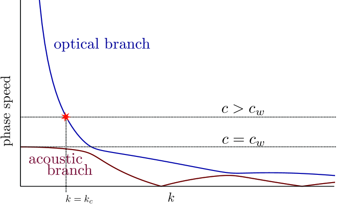
Figure 1. Sketch of the phase speeds for the different branches of the dispersion relation.

In a very rough sense, then, we expect the localized acoustic wave with speed $c$ to excite a mode in the optical branch with wavenumber $k_{c}$. Making this intuition rigorous is, of course, a substantial part of our analysis.

The inequalities in (2.5) imply $\widetilde{\lambda}_{-}(k)<\widetilde{\lambda}_{+}(k)$ for all $k\in{\bf{R}}$. Thus $\widetilde{L}(k)$ is diagonalizable for all $k$. Towards this end, we compute that the eigenvectors of $\widetilde{L}(k)$ are scalar multiples of $\displaystyle\left[\begin{array}[]{c}\widetilde{\beta}(k)\\ \widetilde{\varrho}(k)\end{array}\right]$ (for $\widetilde{\lambda}_{-}(k)$) and $\displaystyle\left[\begin{array}[]{c}\widetilde{\beta}(k)\\ -\widetilde{\varrho}(k)\end{array}\right]$ (for $\widetilde{\lambda}_{+}(k)$).

We can diagonalize $\widetilde{L}$ by dropping these into a matrix. It will be advantageous to renormalize them first, though. Let

$$\widetilde{\gamma}(k):=e^{-ik}+e^{ik}{\widetilde{\varrho}(k)\over\widetilde{\beta}(k)}$$

and put

$$\widetilde{J}_{2}(k):=\left[\begin{array}[]{cc}\widetilde{\gamma}(k)\widetilde{\beta}(k)&\widetilde{\gamma}(k)\widetilde{\beta}(k)\\ \widetilde{\gamma}(k)\widetilde{\varrho}(k)&-\widetilde{\gamma}(k)\widetilde{\varrho}(k)\end{array}\right].$$

Its inverse is

$$\widetilde{J}_{1}(k):=\widetilde{J}_{2}^{-1}(k)=\left[\begin{array}[]{cc}(2\widetilde{\gamma}(k)\widetilde{\beta}(k))^{-1}&(2\widetilde{\gamma}(k)\widetilde{\varrho}(k))^{-1}\\ (2\widetilde{\gamma}(k)\widetilde{\beta}(k))^{-1}&-(2\widetilde{\gamma}(k)\widetilde{\varrho}(k))^{-1}\end{array}\right].$$

Then we have

$$\widetilde{J}_{1}(k)\widetilde{L}(k)\widetilde{J_{2}}(k)=\widetilde{\Lambda}(k):=\left[\begin{array}[]{cc}\widetilde{\lambda}_{-}(k)&0\\ 0&\widetilde{\lambda}_{+}(k)\end{array}\right].$$

The reason we choose to normalize the eigenvectors with $\widetilde{\gamma}$ is obviously non-obvious. Here is what is special about $\widetilde{\gamma}$:

(2.11) $$\widetilde{\gamma}(-k)\widetilde{\beta}(-k)=\widetilde{\gamma}(k)\widetilde{\varrho}(k).$$

This property—easily checked—will imply a certain symmetry below, specifically in the proof of Lemma 4.

A short computation indicates that neither $\widetilde{\gamma}$ nor $\widetilde{\beta}$ vanish when $k\in{\bf{R}}$. In fact, we have:

Corollary 3.

If $w>1$ then there exists $\tau_{1}\in(0,\tau_{0}]$ such that $\widetilde{\gamma}(z)$, $\widetilde{\gamma}^{-1}(z)$, $\widetilde{\beta}(z)$ and $\widetilde{\beta}^{-1}(z)$ are uniformly bounded analytic functions for $z\in\overline{\Sigma}_{\tau_{1}}$. Moreover $\widetilde{J}_{1}(z)$ and $\widetilde{J}_{2}(z)$ are uniformly bounded matrix valued analytic functions for $z\in\overline{\Sigma}_{\tau_{1}}$.

We do not provide a proof, as it is more or less immediate from the definitions and Lemma 2. Note also that

(2.12) $$\widetilde{J}_{1}(0)={1\over 4(1+w)}\left[\begin{array}[]{cr}1&1\\ 1&-1\end{array}\right]\quad\text{and}\quad\widetilde{J}_{2}(0)={2(1+w)}\left[\begin{array}[]{cr}1&1\\ 1&-1\end{array}\right].$$

Since $\widetilde{J}_{1}$ and $\widetilde{J}_{2}$ diagonalize $\widetilde{L}$, we can use Fourier multiplier operators to diagonalize $L$. We use following normalizations and notations for the Fourier transform and its inverse:

$$\widehat{f}(k):={\mathfrak{F}}[f](k):={1\over 2\pi}\int_{\bf{R}}f(x)e^{-ikx}dx\quad\text{and}\quad{\mathchoice{{\ooalign{\hbox{\raise 6.25pt\hbox{\scalebox{1.0}[-1.0]{\lower 6.25pt\hbox{$\displaystyle\widehat{\vrule width=0.0pt,height=4.30554pt\vrule height=0.0pt,width=5.12846pt}$}}}}\cr\hbox{$\displaystyle g$}}}}{{\ooalign{\hbox{\raise 6.25pt\hbox{\scalebox{1.0}[-1.0]{\lower 6.25pt\hbox{$\textstyle\widehat{\vrule width=0.0pt,height=4.30554pt\vrule height=0.0pt,width=5.12846pt}$}}}}\cr\hbox{$\textstyle g$}}}}{{\ooalign{\hbox{\raise 5.81944pt\hbox{\scalebox{1.0}[-1.0]{\lower 5.81944pt\hbox{$\scriptstyle\widehat{\vrule width=0.0pt,height=3.01389pt\vrule height=0.0pt,width=3.58992pt}$}}}}\cr\hbox{$\scriptstyle g$}}}}{{\ooalign{\hbox{\raise 5.53241pt\hbox{\scalebox{1.0}[-1.0]{\lower 5.53241pt\hbox{$\scriptscriptstyle\widehat{\vrule width=0.0pt,height=2.15277pt\vrule height=0.0pt,width=2.56422pt}$}}}}\cr\hbox{$\scriptscriptstyle g$}}}}}(x):={\mathfrak{F}}^{-1}[g](x):=\int_{\bf{R}}g(k)e^{ikx}dk.$$

Likewise, we use the following normalizations and notations for the Fourier series of a $2P$-periodic function:

$$\widehat{f}(k):={1\over 2P}\int_{-P}^{P}f(x)e^{-ik\pi x/P}dx\quad\text{and}\quad{f}(x)=\sum_{k\in{\bf{Z}}}\widehat{f}(k)e^{ik\pi x/P}.$$

We have used the same “hat” notation for the Fourier transform and the coefficients of the Fourier series; context will always make it clear which we mean.

Definition 1.

Suppose that we have $\widetilde{\mu}:{\bf{R}}\to{\bf{C}}$. The “Fourier multiplier with symbol $\widetilde{\mu}$” is defined as follows.

1. If $f:{\bf{R}}\to{\bf{C}}$ has a well-defined Fourier transform then

   (2.13) $$\mu f(x):=\int_{\bf{R}}e^{ikx}\widetilde{\mu}(k)\widehat{f}(k)dk.$$

2. If $f:{\bf{R}}\to{\bf{C}}$ is $2P$-periodic then

   (2.14) $$\mu f(x):=\sum_{k\in{\bf{Z}}}e^{ik\pi x/P}\widetilde{\mu}(k\pi/P)\widehat{f}(k).$$

3. If $f=f_{1}+f_{2}$ where $f_{1}:{\bf{R}}\to{\bf{C}}$ has a well-defined Fourier transform and $f_{2}:{\bf{R}}\to{\bf{C}}$ is $2P$-periodic then we have $\mu f=\mu f_{1}+\mu f_{2}$ where $\mu f_{1}$ is computed with (2.13) and $\mu f_{2}$ is computed with (2.14).

Remark 2.

An alternate way to express (2.14) goes as follows. Since $f(x)$ is $2P$-periodic we know $f(x)=\phi(\omega x)$ for some $2\pi$-periodic function $\phi(y)$ and $\omega=\pi/P$. In this case $\mu f(x)=(\mu^{\omega}\phi)(\omega x)$ where $\mu^{\omega}$ is a Fourier multiplier with symbol $\widetilde{\mu}^{\omega}(k)=\widetilde{\mu}(\omega k)$. The nice thing here is that

$$\mu^{\omega}\phi(y)=\sum_{k\in{\bf{Z}}}e^{iky}\widetilde{\mu}^{\omega}(k)\widehat{\phi}(k),$$

a slightly less complicated formula than (2.14).

Note also that if we put a $2P-$periodic function into the Fourier transform integral ${\mathfrak{F}}$ then we can interpret the output as a distribution. Specifically, it will be a superposition of delta-functions situated on $(\pi/P){\bf{Z}}\subset{\bf{R}}$. In this case we can apply the formula (2.13). The outcome of this coincides exactly with (2.14). In this way we can see that the formula in Part (iii) is the “correct” way to apply Fourier multipliers to sums of decaying and periodic functions.

So let $\lambda_{\pm}$, $\varrho$, $\beta$, $\gamma$, $\Lambda$ and $J_{n}$ be the Fourier multiplier operators with symbols $\widetilde{\lambda}_{\pm}$, $\widetilde{\varrho}$, $\widetilde{\beta}$, $\widetilde{\gamma}$, $\widetilde{\Lambda}$ and $\widetilde{J}_{n}$, respectively. Put ${\bf{p}}:=J_{2}{\bf{h}}$. If ${\bf{p}}$ solves (2.3) then we find that ${\bf{h}}$ solves

(2.15) $$c^{2}{\bf{h}}^{\prime\prime}+\Lambda{\bf{h}}+\Lambda B({\bf{h}},{{\bf{h}}})=0$$

with

$$B({\bf{h}},\grave{{\bf{h}}}):=\left(\begin{array}[]{c}b_{1}({\bf{h}},\grave{{\bf{h}}})\\ b_{2}({\bf{h}},\grave{{\bf{h}}})\end{array}\right):=J_{1}(J_{2}{\bf{h}}.J_{2}\grave{{\bf{h}}}).$$

Written out component-wise this is

(2.16) $$c^{2}h_{1}^{\prime\prime}+\lambda_{-}h_{1}+\lambda_{-}b_{1}({\bf{h}},{\bf{h}})=0\quad\text{and}\quad c^{2}h_{2}^{\prime\prime}+\lambda_{+}h_{2}+\lambda_{+}b_{2}({\bf{h}},{\bf{h}})=0.$$

Remark 3.

Since $\lambda_{-}$ is associated to the acoustic branch of the dispersion relation and $\lambda_{+}$ to the optical branch, we informally think of $h_{1}$ as the “acoustic part” of the solution and $h_{2}$ as the “optical part.” What we shall see down the line is that the dominant part of $h_{1}$ is a $\operatorname{sech}^{2}$ traveling wave, whereas the periodic solutions will be largest in $h_{2}$.

2.2. The Friesecke-Pego cancelation

Applying ${\mathfrak{F}}$ to the first equation in (2.16) gives

(2.17) $$\left(-c^{2}k^{2}+\widetilde{\lambda}_{-}(k)\right)\widehat{h}_{1}+\widetilde{\lambda}_{-}(k)\widehat{b_{1}({\bf{h}},{\bf{h}})}=0.$$

Since $\widetilde{\lambda}_{-}(0)=0$ and is even, it is roughly quadratic in $k$ near the origin. Obviously so is $k^{2}$. Which indicates that we can cancel a $k^{2}$ out of the above if we chose. We do not do precisely this, but instead employ a similar approach inspired by the proof of the existence of low energy solitary waves for monotomic FPU in [FP99].

We know that $\widetilde{\lambda}_{-}(0)=0$ . We also know from (2.6) that $|\widetilde{\lambda}^{\prime}_{-}(k)|\leq 2c_{w}^{2}|k|$. And so the FTOC implies:

(2.18) $$c^{2}k^{2}-\widetilde{\lambda}_{-}(k)>0\quad\text{for all $k\neq 0$ provided $c^{2}\geq c_{w}^{2}$.}$$

This allows us to divide through in (2.17), not by $k^{2}$, but rather by $-c^{2}k^{2}+\widetilde{\lambda}_{-}(k)$.

So put

$$\widetilde{\varpi}_{c}(k):=-{\widetilde{\lambda}_{-}(k)\over c^{2}k^{2}-\widetilde{\lambda}_{-}(k)}.$$

This function has a removable singularity at $k=0$ when $c^{2}>c_{w}^{2}$ and no other singularities for $k\in{\bf{R}}$. Then (2.17) is equivalent to $\displaystyle\widehat{h}_{1}+\widetilde{\varpi}_{c}(k)\widehat{b_{1}({\bf{h}},{\bf{h}})}=0.$

Let $\varpi_{c}f$ be the Fourier multiplier operator with symbol $\widetilde{\varpi}_{c}$. The above reasoning shows we can rewrite (2.16) as

(2.19) $$h_{1}+\varpi_{c}b_{1}({\bf{h}},{\bf{h}})=0\quad\text{and}\quad c^{2}h_{2}^{\prime\prime}+\lambda_{+}h_{2}+\lambda_{+}b_{2}({\bf{h}},{\bf{h}})=0$$

or alternately as:

$${\mathcal{H}}_{c}({\bf{h}}):=\left[\begin{array}[]{cc}1&0\\ 0&c^{2}\partial_{x}^{2}+\lambda_{+}\end{array}\right]{\bf{h}}+\left[\begin{array}[]{cc}\varpi_{c}&0\\ 0&\lambda_{+}\end{array}\right]B({\bf{h}},{\bf{h}})=0.$$

Remark 4.

We will henceforth require $c^{2}>c_{w}^{2}$ so that our map $\varpi_{c}$ is well-defined; this is the technical reason why we look for (and why the authors of [FP99] looked for) nonlinear waves which are supersonic. Unraveling the scalings that lead to (1.3) from (0.1) shows that the traveling wave solutions under investigation here will, in the physical coordinates, travel with a speed faster than $c_{sound}:=\sqrt{k_{s}/\bar{m}}$, where $\bar{m}$ is the average of the two masses.

We have the following nice symmetry result for ${\mathcal{H}}_{c}$.

Lemma 4.

If $h_{1}$ is even and $h_{2}$ is odd, the first and second components of ${{\mathcal{H}}}_{c}({\bf{h}})$ are, respectively, even and odd.

Proof.

For a function $f(y)$ let $Rf(y)=f(-y)$. If $f$ is even then $f=Rf$. If $f$ is odd then $f=-Rf$. If $\mu$ is a Fourier multiplier with symbol $\widetilde{\mu}$ then

(2.20) $$R(\mu f)(x)=(R\mu)Rf(x).$$

By $R\mu$ we mean the Fourier multiplier with symbol $R\widetilde{\mu}(k)=\widetilde{\mu}(-k)$.

If the symbol $\mu$ is even then this implies $R(\mu f)=\mu(Rf).$ This in turn implies that such a $\mu$ will map even functions to even functions and odd functions to odd functions. Thus $\lambda_{\pm}$, $\partial_{x}^{2}$ and $\varpi_{c}$ all “preserve parity.”

Informally, we say ${\bf{h}}\in E\times O$ if $h_{1}$ is even and $h_{2}$ is odd. The preceding comments imply that we will have our result if we can show that $B({\bf{h}},{\bf{h}})$ maps $E\times O$ to itself since the remaining parts of ${\mathcal{H}}_{c}$ will not flip an $E$ to an $O$ or vice versa. Note that ${\bf{h}}\in E\times O$ if and only if $R{\bf{h}}=I_{1}{\bf{h}}$ where $I_{1}=\operatorname{diag}(1,-1)$. Thus our goal is to show that if $R{\bf{h}}=I_{1}{\bf{h}}$ then $RB({\bf{h}},{\bf{h}})=I_{1}B({\bf{h}},{\bf{h}})$.

So suppose that $R{\bf{h}}=I_{1}{\bf{h}}$. Using (2.20) we have $\displaystyle RB({\bf{h}},{\bf{h}})=(RJ_{1})R[(J_{2}{\bf{h}})^{.2}].$ It is easy to see that $R(fg)=RfRg$ and so the above gives $RB({\bf{h}},{\bf{h}})=(RJ_{1})[(R(J_{2}{\bf{h}}))^{.2}].$ Then we use (2.20) again to get $RB({\bf{h}},{\bf{h}})=(RJ_{1})[((RJ_{2})(R{\bf{h}}))^{.2}].$ Since $R{\bf{h}}=I_{1}{\bf{h}}$ we have $RB({\bf{h}},{\bf{h}})=(RJ_{1})[((RJ_{2})(I_{1}{\bf{h}}))^{.2}].$ Then associativity gives:

(2.21) $$RB({\bf{h}},{\bf{h}})=(RJ_{1})[((RJ_{2}I_{1}){\bf{h}})^{.2}].$$

The multiplier for $RJ_{2}$ is, using (2.20),

$$R\widetilde{J}_{2}(k)=\widetilde{J}_{2}(-k)=\left[\begin{array}[]{cc}\widetilde{\gamma}(-k)\widetilde{\beta}(-k)&\widetilde{\gamma}(-k)\widetilde{\beta}(-k)\\ \widetilde{\gamma}(-k)\widetilde{\varrho}(-k)&-\widetilde{\gamma}(-k)\widetilde{\varrho}(-k)\end{array}\right].$$

Now we use the special property of $\widetilde{\gamma}$ in (2.11) to convert this to:

$$R\widetilde{J}_{2}(k)=\left[\begin{array}[]{cc}\widetilde{\gamma}(k)\widetilde{\varrho}(k)&\widetilde{\gamma}(k)\widetilde{\varrho}(k)\\ \widetilde{\gamma}(k)\widetilde{\beta}(k)&-\widetilde{\gamma}(k)\widetilde{\beta}(k)\end{array}\right].$$

If we let $I_{2}:=\left[\begin{array}[]{cc}0&1\\ 1&0\end{array}\right]$ then the above relation implies, after a short calculation, that $R\widetilde{J}_{2}=I_{2}\widetilde{J}_{2}I_{1}.$ Since $\widetilde{J}_{1}=\widetilde{J}_{2}^{-1}$, $I_{1}^{-1}=I_{1}$ and $I_{2}^{-1}=I_{2}$, this gives. $R\widetilde{J}_{1}=I_{1}\widetilde{J}_{1}I_{2}.$

Using these relations in (2.21) gives us $RB({\bf{h}},{\bf{h}})=I_{1}J_{1}I_{2}[(I_{2}J_{2}I_{1}^{2}){\bf{h}})^{.2}].$ Since $I_{1}^{2}$ is the identity this is $RB({\bf{h}},{\bf{h}})=I_{1}J_{1}I_{2}[(I_{2}J_{2}){\bf{h}})^{.2}].$ Also, it is easy to check that $(I_{2}{\bf{f}})^{.2}=I_{2}({\bf{f}}^{.2})$. Thus we have $RB({\bf{h}},{\bf{h}})=I_{1}J_{1}I^{2}_{2}[(J_{2}{\bf{h}})^{.2}].$ Since $I_{2}^{2}$ is the identity this is $RB({\bf{h}},{\bf{h}})=I_{1}J_{1}[(J_{2}{\bf{h}})^{.2}]=I_{1}B({\bf{h}},{\bf{h}}).$ This was our goal and so we are done. ∎

In light of this result, we restrict our attention henceforth to looking for solutions which are even in the first component and odd in the second.

2.3. Long wave scaling

Now make the long wave scaling (inspired by the classical multiscale derivation of the Korteweg-de Vries equation from monotomic FPU in [Kru74])

$$h_{1}(x):=\epsilon^{2}\theta_{1}(\epsilon x),\quad h_{2}:=\epsilon^{2}\theta_{2}(\epsilon x)\quad\text{and}\quad c^{2}=c_{w}^{2}+\epsilon^{2}$$

where $0<\epsilon\ll 1$.

Remark 5.

Note that if $\mu$ is a Fourier multiplier operator with symbol $\widetilde{\mu}(k)$ and if $f(x)=\phi(\omega x)$ then $\mu f(x)=(\mu^{\omega}\phi)(\epsilon x)$ where $\mu^{\omega}$ is a Fourier multiplier with symbol ${\widetilde{\mu}^{\omega}}(k):=\widetilde{\mu}(\omega k).$

After the scaling, (2.19) becomes

(2.22) $$\theta_{1}+\varpi^{\epsilon}b_{1}^{\epsilon}({\boldsymbol{\theta}},{\boldsymbol{\theta}})=0\quad\text{and}\quad\epsilon^{2}(c_{w}^{2}+\epsilon^{2})\theta_{2}^{\prime\prime}+\lambda_{+}^{\epsilon}\theta_{2}+\epsilon^{2}\lambda^{\epsilon}_{+}b^{\epsilon}_{2}({\boldsymbol{\theta}},{\boldsymbol{\theta}})=0$$

with $\displaystyle{\boldsymbol{\theta}}:=\left(\begin{array}[]{c}\theta_{1}\\ \theta_{2}\end{array}\right),$

(2.23) $$\widetilde{\varpi^{\epsilon}}(K):=\epsilon^{2}\widetilde{\varpi}_{{\sqrt{c^{2}_{w}+\epsilon^{2}}}}(\epsilon K)=-{\epsilon^{2}\widetilde{\lambda}_{-}(\epsilon K)\over(c_{w}^{2}+\epsilon^{2})\epsilon^{2}K^{2}-\widetilde{\lambda}_{-}(\epsilon K)},$$

(2.24) $$\widetilde{\lambda}^{\epsilon}_{\pm}(K):=\widetilde{\lambda}_{\pm}(\epsilon K),$$

(2.25) $$\widetilde{J}^{\epsilon}_{j}(K):=\widetilde{J}_{j}(\epsilon K)$$

and

(2.26) $$B^{\epsilon}({\boldsymbol{\theta}},\grave{{\boldsymbol{\theta}}}):=\left(\begin{array}[]{c}b_{1}^{\epsilon}({\boldsymbol{\theta}},\grave{{\boldsymbol{\theta}}})\\ b_{2}^{\epsilon}({\boldsymbol{\theta}},\grave{{\boldsymbol{\theta}}})\end{array}\right):=J^{\epsilon}_{1}\left[J_{2}^{\epsilon}{\boldsymbol{\theta}}.J_{2}^{\epsilon}\grave{{\boldsymbol{\theta}}}\right].$$

Of course $\varpi^{\epsilon}$, $\lambda^{\epsilon}_{\pm}$ and $J_{n}^{\epsilon}$ are Fourier multiplier operators with the symbols taken in the obvious way. Note that since we assume the $\epsilon\in(0,1)$, the scaling implies, via Lemma 2 and Corollary 3, that $\widetilde{\lambda}^{\epsilon}_{\pm}(Z)$ and $\widetilde{J}_{n}^{\epsilon}(Z)$ are analytic for $|\Im(Z)|\leq\tau_{1}\leq\tau_{1}/\epsilon$.

Remark 6.

The equation for $\theta_{2}$ (which is the part associated to the optical branch) is classically singular when $\epsilon\sim 0$ because of the term

$$\epsilon^{2}(c_{w}^{2}+\epsilon^{2})\theta_{2}^{\prime\prime}.$$

Had we not performed the Friesecke-Pego cancelation earlier, the $\theta_{1}$ equation would have a similarly singular term. But the cancelation desingularizes that equation as we shall demonstrate below. Of course this why they made that cancelation in their work [FP99] and why we do so here. But because $\widetilde{\lambda}_{+}(0)\neq 0$ there is no chance to make a similar cancelation in the second component.

We can write (2.22) as:

(2.27) $$\Theta_{\epsilon}({\boldsymbol{\theta}}):=\left[\begin{array}[]{cc}1&0\\ 0&\epsilon^{2}(c_{w}^{2}+\epsilon^{2})\partial_{X}^{2}+\lambda_{+}^{\epsilon}\end{array}\right]{\boldsymbol{\theta}}+\left[\begin{array}[]{cc}\varpi^{\epsilon}&0\\ 0&\epsilon^{2}\lambda^{\epsilon}_{+}\end{array}\right]B^{\epsilon}({\boldsymbol{\theta}},{\boldsymbol{\theta}})=0.$$

The long wave scaling does not effect the symmetry mapping properties that ${\mathcal{H}}_{c}$ had. To wit:

Lemma 5.

If $\theta_{1}$ is even and $\theta_{2}$ is odd, the first and second components of ${\Theta}_{\epsilon}({\bf{h}})$ are, respectively, even and odd.

3. The formal long wave limit

In this section we naively set $\epsilon=0$ in (2.22). This is mostly routine. For instance, given the definitions in (2.24) and (2.25), we set $\widetilde{\lambda}_{+}^{0}(K):=\widetilde{\lambda}_{+}(0)$ and $\widetilde{J}^{0}_{j}(K):=\widetilde{J}_{j}(0)$. So we define, (using (2.12)):

$$\lambda^{0}_{+}:=2+2w,\quad J^{0}_{1}:={1\over 4(1+w)}\left[\begin{array}[]{cr}1&1\\ 1&-1\end{array}\right]\quad\text{and}\quad J^{0}_{2}:=2(1+w)\left[\begin{array}[]{rr}1&1\\ 1&-1\end{array}\right].$$

This in turn leads to the definition

$$B^{0}({\boldsymbol{\theta}},\grave{{\boldsymbol{\theta}}}):=\left(\begin{array}[]{c}b_{1}^{0}({\boldsymbol{\theta}},\grave{{\boldsymbol{\theta}}})\\ b_{2}^{0}({\boldsymbol{\theta}},\grave{{\boldsymbol{\theta}}})\end{array}\right):=J^{0}_{1}\left[J_{2}^{0}{\boldsymbol{\theta}}.J_{2}^{0}\grave{{\boldsymbol{\theta}}}\right]=2(1+w)\left(\begin{array}[]{c}\theta_{1}\grave{\theta}_{1}+\theta_{2}\grave{\theta}_{2}\\ \theta_{1}\grave{\theta}_{2}+\theta_{2}\grave{\theta}_{1}\end{array}\right).$$

Blindly setting $\epsilon=0$ in $\widetilde{\varpi}^{\epsilon}(K)$ will not work; a “$0/0$” situation occurs. Computing the Maclaurin expansion of $\widetilde{\lambda}_{+}(k)$ gives

$$\widetilde{\lambda}_{-}(k)=c_{w}^{2}k^{2}-\alpha_{w}k^{4}+\cdots$$

where

$$\alpha_{w}:={c_{w}^{2}\over 3}{1-w+w^{2}\over(1+w)^{2}}>0.$$

Thus we have

$$\widetilde{\varpi}^{\epsilon}(K)=-{\epsilon^{2}\widetilde{\lambda}_{-}(\epsilon K)\over(c_{w}^{2}+\epsilon^{2})\epsilon^{2}K^{2}-\widetilde{\lambda}_{-}(\epsilon K)}=-{\epsilon^{4}c_{w}^{2}K^{2}+{\mathcal{O}}_{f}(\epsilon^{6})\over(c_{w}^{2}+\epsilon^{2})\epsilon^{2}K^{2}-\epsilon^{2}c_{w}^{2}K^{2}+\alpha_{w}\epsilon^{4}K^{4}+{\mathcal{O}}_{f}(\epsilon^{6})}$$

By “${\mathcal{O}}_{f}(\epsilon^{n})$” we mean terms which are formally of order $\epsilon^{n}$.

After some cancelations this becomes

$$\widetilde{\varpi}^{\epsilon}(K)=-{\epsilon^{4}c_{w}^{2}K^{2}+{\mathcal{O}}_{f}(\epsilon^{6})\over\epsilon^{4}K^{2}+\alpha_{w}\epsilon^{4}K^{4}+{\mathcal{O}}_{f}(\epsilon^{6})}=-{c_{w}^{2}K^{2}+{\mathcal{O}}_{f}(\epsilon^{2})\over K^{2}+\alpha_{w}K^{4}+{\mathcal{O}}_{f}(\epsilon^{2})}.$$

Now we set $\epsilon=0$ to get

(3.1) $$\widetilde{\varpi}^{0}(K):=-{c_{w}^{2}\over 1+\alpha_{w}K^{2}}\quad\text{and}\quad{\varpi}^{0}:=-c_{w}^{2}(1-\alpha_{w}\partial_{X}^{2})^{-1}.$$

Remark 7.

We will give precise estimates on the operator norms of $\varpi^{\epsilon}-\varpi^{0}$, $\lambda_{+}^{\epsilon}-\lambda_{+}^{0}$ and so on in Section 7.

With all of this, if we put $\epsilon=0$ in (2.22) we arrive at:

$$\theta_{1}-{4w\over 1-\alpha_{w}\partial_{X}^{2}}\left[\theta_{1}^{2}+\theta_{2}^{2}\right]=0\quad\text{and}\quad(2+2w)\theta_{2}=0.$$

To solve this we take $\theta_{2}=0$ and $\theta_{1}$ a solution of

$$\theta_{1}-{4w\over 1-\alpha_{w}\partial_{X}^{2}}\left[\theta_{1}^{2}\right]=0.$$

Applying $1-\alpha_{w}\partial_{X}^{2}$ to the above results in

(3.2) $$\alpha_{w}\theta_{1}^{\prime\prime}-\theta_{1}+4w\theta_{1}^{2}=0.$$

This is a rescaling of the nonlinear differential equation whose solutions give the profile for the KdV solitary waves. It has an explicit solution given by

(3.3) $$\theta_{1}(X)=\sigma(X):=\sigma_{0}\operatorname{sech}^{2}(2q_{0}X)\quad\text{where}\quad\sigma_{0}:={3\over 8w}\quad\text{and}\quad q_{0}:={1\over 2\sqrt{\alpha_{w}}}.$$

Note that if we put ${\boldsymbol{\sigma}}:=(\sigma,0)^{t}$ then we have shown:

(3.4) $$\sigma+\varpi^{0}b_{1}^{0}({\boldsymbol{\sigma}},{\boldsymbol{\sigma}})=0.$$

Remark 8.

Observe that in the limit $\epsilon\to 0^{+}$ the part of the solution associated to optical branch, $\theta_{2}$, plays no role. All the action is happening for the acoustic part $\theta_{1}$.

Remark 9.

In [GMWZ14] the authors use homogenization theory to show that solutions of (1.3) with initial data of the form $r(j,0)=\epsilon^{2}R(\epsilon j)$ and $\dot{x}(j,0)=\epsilon^{2}V(\epsilon j)$ are well-approximated over long times by a pair of solutions of KdV. Specifically they show that

$$r(j,t)=\epsilon^{2}U_{-}(\epsilon(j-c_{w}t),\epsilon^{3}t)+\epsilon^{2}U_{+}(\epsilon(j+c_{w}t),\epsilon^{3}t)+{\mathcal{O}}(\epsilon^{3/2})\quad\text{for all $|t|\leq C\epsilon^{-3}$}$$

where $U_{\pm}$ solve the KdV equations

$$\pm\partial_{T}U_{\pm}+\alpha_{w}\partial_{X}^{3}U_{\pm}+4w\partial_{X}(U^{2}_{\pm})=0.$$

Making a traveling wave ansatz for these of the form $U_{\pm}(X,T)=\theta(X\mp T)$ results in (3.2); the coefficients match exactly. Which is to say the results here are consistent with those in [GMWZ14].

4. Periodic solutions

In this section we prove the existence of spatially periodic solutions of (2.22). To this end, we first compute the linearization of that equation about ${\boldsymbol{\theta}}(X)=0$ to get

$$\theta_{1}=0\quad\text{and}\quad\epsilon^{2}(c_{w}^{2}+\epsilon^{2})\theta_{2}^{\prime\prime}+\lambda_{+}^{\epsilon}\theta_{2}=0.$$

We are looking for solutions where $\theta_{2}$ is odd and periodic. Thus we can take $\theta_{2}(X)=\sin(K_{\epsilon}X)$ for some $K_{\epsilon}\in{\bf{R}}$. Inserting this into the second equation above, and recalling that $\lambda_{+}^{\epsilon}$ is a Fourier multiplier operator with symbol $\widetilde{\lambda}_{+}(\epsilon K)$, gives

$$\epsilon^{2}(c_{w}^{2}+\epsilon^{2})K_{\epsilon}^{2}-\widetilde{\lambda}_{+}(\epsilon K_{\epsilon})=0.$$

If we put $c=c_{\epsilon}:=\sqrt{c_{w}^{2}+\epsilon^{2}}$ and

$$K_{\epsilon}:=k_{c_{\epsilon}}/\epsilon,$$

this last equation is exactly (2.7). Which is to say, by virtue of Part (vi) of Lemma 2, that $K_{\epsilon}$ is its unique nonnegative solution.

Thus we have odd periodic solutions of the the linearization of (2.22) of the form

$${\boldsymbol{\theta}}(X)={\boldsymbol{\nu}}_{\epsilon}(X):=\sin(K_{\epsilon}X){\bf{j}}.$$

We can extend the existence of periodic solutions for the linear problem to the full nonlinear problem (2.22) by means of the technique of “bifurcation from a simple eigenvalue,” developed by Crandall & Rabinowitz in [CR71] and Zeidler in [Zei95]. Here is what we find:

Theorem 6.

For all $w>1$ there exist $\epsilon_{0}>0$, $a_{0}>0$ and $0<C_{1}<C_{2}$ such the following holds for all for $\epsilon\in(0,\epsilon_{0})$. There exist maps

(4.1) $$\begin{split}K^{a}_{\epsilon}&:[-a_{0},a_{0}]\longrightarrow{\bf{R}}\\ \psi_{\epsilon,1}^{a}&:[-a_{0},a_{0}]\longrightarrow C^{\infty}_{\text{per}}\cap\left\{\text{even functions}\right\}\\ \psi_{\epsilon,2}^{a}&:[-a_{0},a_{0}]\longrightarrow C^{\infty}_{\text{per}}\cap\left\{\text{odd functions}\right\}\end{split}$$

with the following properties.

1. Putting

   $${\boldsymbol{\theta}}(X)=a{\boldsymbol{\varphi}}^{a}_{\epsilon}(X):=a\left(\begin{array}[]{c}0\\ \sin(K_{\epsilon}^{a}X)\end{array}\right)+a\left(\begin{array}[]{c}\psi^{a}_{\epsilon,1}(K_{\epsilon}^{a}X)\\ \psi^{a}_{\epsilon,1}(K_{\epsilon}^{a}X)\end{array}\right)=:a{{\boldsymbol{\nu}}}(K_{\epsilon}^{a}X)+{\boldsymbol{\psi}}^{a}_{\epsilon}(K_{\epsilon}^{a}X)$$

   solves (2.22) for all $|a|\leq a_{0}$.

2. $K_{\epsilon}^{0}=K_{\epsilon}$ where $K_{\epsilon}$ is the unique positive solution of

   (4.2) $$\widetilde{\xi}_{\sqrt{c_{w}^{2}+\epsilon^{2}}}(\epsilon{K}):=-\epsilon^{2}(c_{w}^{2}+\epsilon^{2})K^{2}+\widetilde{\lambda}_{+}(\epsilon K)=0.$$

   Moreover $K_{\epsilon}={\mathcal{O}}(1/\epsilon)$ in the sense that

   $$C_{1}/\epsilon<K_{\epsilon}<C_{2}/\epsilon\quad\text{ for all $\epsilon\in(0,\epsilon_{0})$}.$$

3. $\psi^{0}_{\epsilon,1}=\psi^{0}_{\epsilon,2}=0$.

4. $\displaystyle\int_{-\pi}^{\pi}\psi^{a}_{\epsilon,2}(y)\sin(y)\ dy=0$ for all $|a|\leq a_{0}$.

5. For all $r\geq 0$, there exists $C_{r}>0$ such that for all $|a|,|{\grave{a}}|\leq a_{0}$ we have

   (4.3) $$\left|\epsilon K_{\epsilon}^{a}\right|+\left\|{\boldsymbol{\psi}}^{a}_{\epsilon}\right\|_{C^{r}_{\text{per}}\times C^{r}_{\text{per}}}\leq C_{r}$$

   and

   (4.4) $$\left|K_{\epsilon}^{a}-K_{\epsilon}^{\grave{a}}\right|+\left\|{\boldsymbol{\psi}}^{a}_{\epsilon}-{\boldsymbol{\psi}}^{\grave{a}}_{\epsilon}\right\|_{C^{r}_{\text{per}}\times C^{r}_{\text{per}}}\leq C_{r}|a-{\grave{a}}|.$$

The remainder of Section 4 is dedicated to the proof of this theorem.

4.1. Frequency freezing

We begin by making the additional scaling

(4.5) $${\boldsymbol{\theta}}(X):={\boldsymbol{\phi}}(\omega{X})\quad\text{ with }{\boldsymbol{\phi}}:=\left(\begin{array}[]{c}\phi_{1}\\ \phi_{2}\end{array}\right),\ \omega\in{\bf{R}},$$

where ${\boldsymbol{\phi}}(Y)$ is $2\pi$-periodic. By Remark 5, our system (2.27) becomes

(4.6) $$\boldsymbol{\Phi}_{\epsilon}({\boldsymbol{\phi}},\omega):=\left[\begin{array}[]{cc}1&0\\ 0&\epsilon^{2}\omega^{2}(c_{w}^{2}+\epsilon^{2})\partial_{Y}^{2}+\lambda_{+}^{\epsilon\omega}\end{array}\right]{\boldsymbol{\phi}}+\left[\begin{array}[]{cc}\varpi^{\epsilon,\omega}&0\\ 0&\epsilon^{2}\lambda^{\epsilon\omega}_{+}\end{array}\right]B^{\epsilon\omega}({\boldsymbol{\phi}},{\boldsymbol{\phi}})=0.$$

where $\varpi^{\epsilon,\omega}$ is the multiplier with symbol

$$\widetilde{\varpi}^{\epsilon,\omega}(K):=\widetilde{\varpi}^{\epsilon}(\omega{K}),$$

and the multipliers $\lambda_{+}^{\epsilon\omega}$ and $B^{\epsilon\omega}$ conform to their prior definitions.

Since $B^{\epsilon\omega}$ is quadratic in ${\boldsymbol{\phi}}$, it is easy to see that

$$D_{{\boldsymbol{\phi}}}\boldsymbol{\Phi}_{\epsilon}(0,\omega)=\begin{bmatrix}1&0\\ 0&\epsilon^{2}\omega^{2}(c_{w}^{2}+\epsilon^{2})\partial_{Y}^{2}+\lambda_{+}^{\epsilon\omega}\end{bmatrix}.$$

When $\omega=K_{\epsilon}$, one may show that zero is a simple eigenvalue of $D_{{\boldsymbol{\phi}}}\boldsymbol{\Phi}_{\epsilon}(0,K_{\epsilon})$ when the operator is restricted to a suitable function space; this is essentially just the calculation carried out at the start of this section. Consequently, the classical bifurcation results in [CR71] and [Zei95] can be used to show that there exists a nontrivial family of solutions to $\boldsymbol{\Phi}_{\epsilon}({\boldsymbol{\phi}},\omega)=0$ branching out of $(0,K_{\epsilon})$. Unfortunately, those classical results do not provide, in an easy way, estimates on the solution which are uniform in $\epsilon$. And so, while our strategy is modeled on the proofs of the results in [CR71] and [Zei95], we carry out the proof from scratch and always with our eyes on how quantities depend on $\epsilon$. Our first step is to convert (4.6) to a fixed point equation.

4.2. Conversion to a fixed-point problem

Let

$$\mathcal{Y}=(H_{{\text{per}}}^{2}\cap\{\text{even functions}\})\times(H_{{\text{per}}}^{2}\cap\{\text{odd functions}\}),$$

where $H_{{\text{per}}}^{r}$ is the Sobolev space of $2\pi$-periodic functions $\phi$ such that

$$\|\phi\|_{H_{{\text{per}}}^{r}}:=\left(\sum_{k\in{\bf{Z}}}(1+k^{2})^{r}|\widehat{\phi}(k)|^{2}\right)^{1/2}<\infty.$$

With ${\boldsymbol{\nu}}(Y):=\sin(Y)\bf{j}$, we have the direct sum decomposition $\mathcal{Y}=\mathcal{N}\oplus\mathcal{Z}$, where $\mathcal{Z}\subseteq\mathcal{Y}$ is the orthogonal complement of $\mathcal{N}:=\operatorname{span}(\{{\boldsymbol{\nu}}\})$ in the standard $H_{{\text{per}}}^{2}\times H_{{\text{per}}}^{2}$ inner product, i.e.,

$$\left\langle{\boldsymbol{\phi}},{\boldsymbol{\psi}}\right\rangle_{H_{{\text{per}}}^{2}\times H_{{\text{per}}}^{2}}:=\left\langle\phi_{1},\psi_{1}\right\rangle_{H_{{\text{per}}}^{2}}+\left\langle\phi_{2},\psi_{2}\right\rangle_{H_{{\text{per}}}^{2}}\quad\text{ with }\quad\left\langle\phi,\psi\right\rangle_{H_{{\text{per}}}^{2}}:=\sum_{k\in{\bf{Z}}}(1+k^{2})^{2}\widehat{\phi}(k)\overline{\widehat{\psi}(k)}.$$

We may then write any ${\boldsymbol{\phi}}\in\mathcal{Y}$ as

(4.7) $${\boldsymbol{\phi}}=a{\boldsymbol{\nu}}+a{\boldsymbol{\psi}}\quad\text{ for some }\quad a\in{\bf{R}},\ {\boldsymbol{\psi}}\in\mathcal{Z}.$$

Observe that if ${\boldsymbol{\psi}}\in\mathcal{Z}$, then $\widehat{{\boldsymbol{\psi}}}(\pm 1)\cdot{\bf{j}}=0$. Set

(4.8) $${\mathcal{X}}=\mathcal{Z}\times{\bf{R}}.$$

Since the trivial solution ${\boldsymbol{\phi}}=0$ already solves (4.6) for any choice of $\omega$, we will assume $a\neq 0$. After factoring and dividing by $a$, the problem

$$\boldsymbol{\Phi}_{\epsilon}({\boldsymbol{\phi}},K_{\epsilon}+t)=\boldsymbol{\Phi}_{\epsilon}(a{\boldsymbol{\nu}}+a{\boldsymbol{\psi}},K_{\epsilon}+t)=0$$

becomes

(4.9) $$\psi_{1}+a\varpi^{\epsilon,{K_{\epsilon}}+t}b_{1}^{\epsilon({K_{\epsilon}}+t)}({\boldsymbol{\nu}}+{\boldsymbol{\psi}},{\boldsymbol{\nu}}+{\boldsymbol{\psi}})=0$$

and

(4.10) $$(\epsilon^{2}({K_{\epsilon}}+t)^{2}(c_{w}^{2}+\epsilon^{2})\partial_{Y}^{2}+\lambda_{+}^{\epsilon({K_{\epsilon}}+t)})(\sin(Y)+\psi_{2})+a\epsilon^{2}\lambda_{+}^{\epsilon({K_{\epsilon}}+t)}b_{2}^{\epsilon({K_{\epsilon}}+t)}({\boldsymbol{\nu}}+{\boldsymbol{\psi}},{\boldsymbol{\nu}}+{\boldsymbol{\psi}})=0.$$

Let $\Pi_{1}$ be the Fourier multiplier with symbol

$$\widetilde{\Pi}_{1}:=\begin{cases}1,&|k|=1\\ 0,&|k|\neq 1\end{cases}$$

and set $\Pi_{2}=1-\Pi_{1}$. Then (4.9) and (4.10) are equivalent to

(4.11) $$\psi_{1}+a\varpi^{\epsilon,{K_{\epsilon}}+t}b_{1}^{\epsilon({K_{\epsilon}}+t)}({\boldsymbol{\nu}}+{\boldsymbol{\psi}},{\boldsymbol{\nu}}+{\boldsymbol{\psi}})=0,$$

(4.12) $$(\epsilon^{2}({K_{\epsilon}}+t)^{2}(c_{2}^{2}+\epsilon^{2})\partial_{X}^{2}+\lambda_{+}^{\epsilon({K_{\epsilon}}+t)})\sin(Y)\!+\!a\epsilon^{2}\Pi_{1}\lambda_{+}^{\epsilon({K_{\epsilon}}+t)}b_{2}^{\epsilon({K_{\epsilon}}+t)}({\boldsymbol{\nu}}+{\boldsymbol{\psi}},{\boldsymbol{\nu}}+{\boldsymbol{\psi}})=0$$

and

(4.13) $$(\epsilon^{2}({K_{\epsilon}}+t)^{2}(c_{2}^{2}+\epsilon^{2})\partial_{X}^{2}+\lambda_{+}^{\epsilon({K_{\epsilon}}+t)})\psi_{2}+a\epsilon^{2}\Pi_{2}\lambda_{+}^{\epsilon({K_{\epsilon}}+t)}b_{2}^{\epsilon({K_{\epsilon}}+t)}({\boldsymbol{\nu}}+{\boldsymbol{\psi}},{\boldsymbol{\nu}}+{\boldsymbol{\psi}})=0.$$

Condition (4.11) immediately gives a fixed-point equation for $\psi_{1}$, and we see that (4.12) holds if and only if the Fourier transform of its left side evaluated at $k=\pm 1$ is zero. Because $b_{2}^{\epsilon({K_{\epsilon}}+t)}({\boldsymbol{\nu}}+{\boldsymbol{\psi}},{\boldsymbol{\nu}}+{\boldsymbol{\psi}})$ is odd by (the proof of) Lemma 4, we need only consider this Fourier transform at $k=1$. With

$$\widetilde{\xi}_{\sqrt{c_{w}^{2}+\epsilon^{2}}}(k)=-(c_{w}^{2}+\epsilon^{2})(\epsilon{k})^{2}+\widetilde{\lambda}_{+}(\epsilon{k})$$

as in (4.2) and $c_{\epsilon}:=\sqrt{c_{w}^{2}+\epsilon^{2}}$, set

(4.14) $$\widetilde{\xi}^{\epsilon,t}(k):=\widetilde{\xi}_{c_{\epsilon}}(\epsilon({K_{\epsilon}}+t)k)$$

so that (4.12) is equivalent to

(4.15) $$\frac{1}{2i}\widetilde{\xi}^{\epsilon,t}(1)+a\epsilon^{2}{\mathfrak{F}}\left[\Pi_{1}\lambda_{+}^{\epsilon({K_{\epsilon}}+t)}b_{2}^{\epsilon({K_{\epsilon}}+t)}({\boldsymbol{\nu}}+{\boldsymbol{\psi}},{\boldsymbol{\nu}}+{\boldsymbol{\psi}})\right](1)=0.$$

Taylor’s theorem tells us that

$$\widetilde{\xi}^{\epsilon,1}(1)=\widetilde{\xi}_{c_{\epsilon}}(\epsilon K_{\epsilon}+\epsilon{t})=\widetilde{\xi}_{c_{\epsilon}}^{\prime}(\epsilon K_{\epsilon})(\epsilon{t})+R_{\epsilon}(\epsilon{t})(\epsilon{t})^{2},$$

and Part (vi) of Lemma 2 provides a number $l_{0}>0$ such that

$$|\widetilde{\xi}_{c_{\epsilon}}^{\prime}(\epsilon{K_{\epsilon}})|\geq l_{0}$$

for all $\epsilon$ sufficiently close to zero. So, we may rewrite (4.15) as

(4.16) $$t=-\frac{\epsilon}{\widetilde{\xi}_{c_{\epsilon}}^{\prime}(\epsilon{K_{\epsilon}})}R_{\epsilon}(\epsilon{t})t^{2}-\frac{2i\epsilon{a}}{\widetilde{\xi}_{c_{\epsilon}}^{\prime}(\epsilon{K_{\epsilon}})}{\mathfrak{F}}\left[\Pi_{1}\lambda_{+}^{\epsilon({K_{\epsilon}}+t)}b_{2}^{\epsilon({K_{\epsilon}}+t)}({\boldsymbol{\nu}}+{\boldsymbol{\psi}},{\boldsymbol{\nu}}+{\boldsymbol{\psi}})\right](1)$$

Finally, we will show that $\widetilde{\xi}^{\epsilon,t}(k)\neq 0$ for $k\neq\pm 1$, which means that the multiplier $(\xi^{\epsilon,t})^{-1}$ with symbol $(\widetilde{\xi}^{\epsilon,t})^{-1}$ is well-defined on the range of $\Pi_{2}$ for suitably small $\epsilon$ and $t$. Then (4.13) becomes

(4.17) $$\psi_{2}=-a\epsilon^{2}\left(\xi^{\epsilon,t}\right)^{-1}\Pi_{2}\lambda_{+}^{\epsilon({K_{\epsilon}}+t)}b_{2}^{\epsilon({K_{\epsilon}}+t)}({\boldsymbol{\nu}}+{\boldsymbol{\psi}},{\boldsymbol{\nu}}+{\boldsymbol{\psi}}).$$

We have arrived at our ultimate fixed-point problem. Set ${\boldsymbol{\Psi}}_{\epsilon}:=(\Psi_{\epsilon,1},\Psi_{\epsilon,2},\Psi_{\epsilon,3})$ with

$$\Psi_{\epsilon,1}({\boldsymbol{\psi}},t,a) :=-a\varpi^{\epsilon,{K_{\epsilon}}+t}b_{1}^{\epsilon({K_{\epsilon}}+t)}({\boldsymbol{\nu}}+{\boldsymbol{\psi}},{\boldsymbol{\nu}}+{\boldsymbol{\psi}})$$

$$\Psi_{\epsilon,2}({\boldsymbol{\psi}},t,a) :=-a\epsilon^{2}(\xi^{\epsilon,t})^{-1}\Pi_{2}\lambda_{+}^{\epsilon({K_{\epsilon}}+t)}b_{2}^{\epsilon({K_{\epsilon}}+t)}({\boldsymbol{\nu}}+{\boldsymbol{\psi}},{\boldsymbol{\nu}}+{\boldsymbol{\psi}})$$

$$\Psi_{\epsilon,3}({\boldsymbol{\psi}},t,a) :=-\frac{\epsilon}{\widetilde{\xi}_{c_{\epsilon}}^{\prime}(\epsilon{K_{\epsilon}})}R_{\epsilon}(\epsilon{t})t^{2}-\frac{2i\epsilon{a}}{\widetilde{\xi}_{c_{\epsilon}}^{\prime}(\epsilon{K_{\epsilon}})}{\mathfrak{F}}\big{[}\Pi_{1}\lambda_{+}^{\epsilon({K_{\epsilon}}+t)}b_{2}^{\epsilon({K_{\epsilon}}+t)}({\boldsymbol{\nu}}+{\boldsymbol{\psi}},{\boldsymbol{\nu}}+{\boldsymbol{\psi}})\big{]}\!(1)$$

We will solve this problem by applying the following lemma, whose proof is given in Section 4.4, to the map ${\boldsymbol{\Psi}}_{\epsilon}$ for $\epsilon$ sufficiently small.

Lemma 7.

Let ${\mathcal{X}}$ be a Banach space and let $\mathcal{B}(r)=\{x\in{\mathcal{X}}:\|x\|\leq r\}$. For $0<\epsilon<\epsilon_{0}$ let $F_{\epsilon}\colon{\mathcal{X}}\times{\bf{R}}\to{\mathcal{X}}$ be maps with the property that for some $C_{1},a_{1},r_{1}>0$, if $x,y\in\mathcal{B}(r_{1})$ and $|a|\leq a_{1}$, then

(4.18) $$\sup_{0<\epsilon<\epsilon_{0}}\|F_{\epsilon}(x,a)\| \leq C_{1}\left(|a|+|a|\|x\|+\|x\|^{2}\right)$$

(4.19) $$\sup_{0<\epsilon<\epsilon_{0}}\|F_{\epsilon}(x,a)-F_{\epsilon}(y,a)\| \leq C_{1}\left(|a|+\|x\|+\|y\|\right)\|x-y\|$$

Then there exist $a_{0}\in(0,a_{1}],r_{0}\in(0,r_{1}]$ such that for each $0<\epsilon<\epsilon_{0}$ and $|a|\leq a_{0}$, there is a unique $x_{\epsilon}^{a}\in\mathcal{B}(r_{0})$ such that $F_{\epsilon}(x_{\epsilon}^{a},a)=x_{\epsilon}^{a}$.

Suppose as well that the maps $F_{\epsilon}(\cdot,a)$ are Lipschitz on $\mathcal{B}(r_{0})$ uniformly in $a$ and $\epsilon$, i.e., there is $L_{1}>0$ such that

(4.20) $$\sup_{\begin{subarray}{c}0<\epsilon<\epsilon_{0}\\ \|x\|\leq r_{0}\end{subarray}}\|F_{\epsilon}(x,a)-F_{\epsilon}(x,\grave{a})\|\leq L_{1}|a-\grave{a}|$$

for all $|a|,|\grave{a}|\leq a_{0}$. Then the mappings $[-a_{0},a_{0}]\to{\mathcal{X}}\colon a\mapsto x_{\epsilon}^{a}$ are also uniformly Lipschitz; that is, there is $L_{0}>0$ such that

(4.21) $$\sup_{0<\epsilon<\epsilon_{0}}\|x_{\epsilon}^{a}-x_{\epsilon}^{\grave{a}}\|\leq L_{0}|a-\grave{a}|$$

for all $|a|,|\grave{a}|\leq a_{1}$.

4.3. Application of Lemma 7

We begin with a general observation about Fourier multipliers. The proof of this lemma follows from direct calculations with the norm

$$\|\psi\|_{H_{{\text{per}}}^{r}}^{2}=\sum_{k\in{\bf{Z}}}(1+k^{2})^{r}|\widehat{\psi}(k)|^{2},$$

and so we omit it. Throughout this section, we denote by ${\bf{B}}(\mathcal{U},\mathcal{V})$ the space of bounded linear operators between normed spaces $\mathcal{U}$ and $\mathcal{V}$ and set ${\bf{B}}(\mathcal{U}):={\bf{B}}(\mathcal{U},\mathcal{U})$.

Lemma 8.

Let $\mu$ be a Fourier multiplier with symbol $\widetilde{\mu}\in L^{\infty}({\bf{R}})$ and let $\omega\in{\bf{R}}$. As in Remark 5, let $\mu^{\omega}$ be the Fourier multiplier with symbol $\widetilde{\mu}^{\omega}(k)=\widetilde{\mu}(\omega{k})$. Then

1. $\sup_{r,\omega\in{\bf{R}}}\|\mu^{\omega}\|_{{\bf{B}}(H_{{\text{per}}}^{r})}\leq\|\widetilde{\mu}\|_{L^{\infty}({\bf{R}})}.$

2. If $\widetilde{\mu}$ is Lipschitz, i.e., there is $\operatorname{Lip}(\widetilde{\mu})>0$ such that $|\widetilde{\mu}(k)-\widetilde{\mu}(\grave{k})|\leq\operatorname{Lip}(\widetilde{\mu})|k-\grave{k}|$, then

   $$\|(\mu^{\omega}-\mu^{\grave{\omega}})\psi\|_{H_{{\text{per}}}^{r}}\leq\operatorname{Lip}(\widetilde{\mu})|\omega-\grave{\omega}|\|\psi\|_{H_{{\text{per}}}^{r+1}}$$

   for all $\omega,\grave{\omega},r\in{\bf{R}}$ and $\psi\in H_{{\text{per}}}^{r+1}$.

3. If there exist $C,p>0$ such that

   $$|\widetilde{\mu}(k)|\leq\frac{C}{(1+k^{2})^{p}}$$

   for all $k\in{\bf{R}}$, then $\|\mu\|_{{\bf{B}}(H_{{\text{per}}}^{r},H_{{\text{per}}}^{r+2p})}\leq C$.

Remark 10.

Informally, Part (ii) of Lemma 8 means that taking a Lipschitz estimate for the map $\omega\mapsto\mu^{\omega}$ costs us a derivative.

The following two lemmas on the Fourier multipliers $\varpi^{\epsilon,K_{\epsilon}+t}$ and $(\xi^{\epsilon,t})^{-1}\Pi_{2}$ are the keys to our application of Lemma 7 to the maps ${\boldsymbol{\Psi}}_{\epsilon}$. They follow directly from the corresponding results for the symbols $\widetilde{\varpi}^{\epsilon,K_{\epsilon}+t}$ and $(\widetilde{\xi}^{\epsilon,t})^{-1}$, which are stated below as Lemmas 11 and 12 and proved in Section 9.2.

Lemma 9.

1. There exist $\epsilon_{11},C_{\varpi\max}>0$ such that

   $$\sup_{\begin{subarray}{c}0<\epsilon<\epsilon_{11}\\ |t|\leq 1\\ r\in{\bf{R}}\end{subarray}}\|\varpi^{\epsilon,K_{\epsilon}+t}\|_{{\bf{B}}(H_{{\text{per}}}^{r},H_{{\text{per}}}^{r+2})}\leq C_{\varpi\max}.$$

2. There exists $C_{\varpi\operatorname{Lip}}>0$ such that if $|t|,|\grave{t}|\leq 1$, then

   $$\sup_{\begin{subarray}{c}0<\epsilon<\epsilon_{11}\\ r\in{\bf{R}}\end{subarray}}\|\varpi^{\epsilon,K_{\epsilon}+t}-\varpi^{\epsilon,K_{\epsilon}+\grave{t}}\|_{{\bf{B}}(H_{{\text{per}}}^{r})}\leq C_{\varpi\operatorname{Lip}}|t-\grave{t}|.$$

Lemma 10.

1. There exist $\epsilon_{12},C_{\xi\max}>0$ such that

   $$\sup_{\begin{subarray}{c}0<\epsilon<\epsilon_{12}\\ |t|\leq 1\\ r\in{\bf{R}}\end{subarray}}\|\epsilon^{2}(\xi^{\epsilon,t})^{-1}\Pi_{2}\|_{{\bf{B}}(H_{{\text{per}}}^{r},H_{{\text{per}}}^{r+2})}\leq C_{\xi\max}.$$

2. There exists $C_{\xi\operatorname{Lip}}>0$ such that

   $$\sup_{\begin{subarray}{c}0<\epsilon<\epsilon_{12}\\ r\in{\bf{R}}\end{subarray}}\|\epsilon^{2}(\xi^{\epsilon,t})^{-1}\Pi_{2}-\epsilon^{2}(\xi^{\epsilon,t})^{-1}\Pi_{2}\|_{{\bf{B}}(H_{{\text{per}}}^{r})}\leq C_{\xi\operatorname{Lip}}|t-\grave{t}|$$

   for all $|t|,|\grave{t}|\leq 1$.

Lemma 11.

There exists $\epsilon_{11}>0$ such that the following hold.

1. There is $C_{\widetilde{\varpi}\max}>0$ such that

   (4.22) $$\sup_{\begin{subarray}{c}0<\epsilon<\epsilon_{11}\\ k\in{\bf{Z}}\\ |t|\leq 1\end{subarray}}|\widetilde{\varpi}^{\epsilon,K_{\epsilon}+t}(k)|\leq\frac{C_{\widetilde{\varpi}\max}}{1+k^{2}}.$$

2. There is $C_{\widetilde{\varpi}\operatorname{Lip}}>0$ such that

   (4.23) $$\sup_{\begin{subarray}{c}0<\epsilon<\epsilon_{11}\\ k\in{\bf{Z}}\end{subarray}}|\widetilde{\varpi}^{\epsilon,K_{\epsilon}+t}(k)-\widetilde{\varpi}^{\epsilon,K_{\epsilon}+\grave{t}}(k)|\leq C_{\widetilde{\varpi}\operatorname{Lip}}|t-\grave{t}|$$

   for all $|t|,|\grave{t}|\leq 1$.

Lemma 12.

There exists $\epsilon_{12}>0$ such that the following hold.

1. There is $C_{\widetilde{\xi}\max}>0$ such that

   (4.24) $$\sup_{\begin{subarray}{c}0<\epsilon<\epsilon_{12}\\ k\in{\bf{Z}}\setminus\{-1,1\}\\ |t|\leq 1\end{subarray}}\left|\frac{1}{\widetilde{\xi}^{\epsilon,t}(k)}\right|\leq\frac{C_{\widetilde{\xi}\max}}{1+k^{2}}.$$

2. There is $C_{\widetilde{\xi}\operatorname{Lip}}>0$ such that

   (4.25) $$\sup_{\begin{subarray}{c}0<\epsilon<\epsilon_{0}\\ k\in{\bf{Z}}\setminus\{-1,1\}\end{subarray}}\left|\frac{1}{\widetilde{\xi}^{\epsilon,t}(k)}-\frac{1}{\widetilde{\xi}^{\epsilon,\grave{t}}(k)}\right|\leq C_{\widetilde{\xi}\operatorname{Lip}}|t-\grave{t}|.$$

Last, Taylor’s theorem provides the following useful decomposition of $\widetilde{\xi}^{\epsilon,t}$, which we prove in Section 9.2.

Lemma 13.

For $0<\epsilon<\epsilon_{12}$ and $\tau\in{\bf{R}}$, we have

(4.26) $$\widetilde{\xi}_{c_{\epsilon}}(\epsilon{K_{\epsilon}}+\tau)=\widetilde{\xi}_{c_{\epsilon}}^{\prime}(\epsilon{K_{\epsilon}})\tau+R_{\epsilon}(\tau)\tau^{2},$$

where the functions $R_{\epsilon}$ have the following property: there exist $C_{R\max},C_{R\operatorname{Lip}}>0$ such that when $0<\epsilon<\epsilon_{12}$,

(4.27) $$\sup_{0<\epsilon<\epsilon_{12}}|R_{\epsilon}(\tau)|\leq C_{R\max}\quad\text{and}\quad\sup_{0<\epsilon<\epsilon_{12}}|R_{\epsilon}(\tau)-R_{\epsilon}(\grave{\tau})|\leq C_{R\operatorname{Lip}}|\tau-\grave{\tau}|$$

for all $\tau,\grave{\tau}\in{\bf{R}}$.

We are now ready to apply Lemma 7 to our map ${\boldsymbol{\Psi}}_{\epsilon}$.

Proposition 14.

Let $\epsilon_{0}=\min\{\epsilon_{11},\epsilon_{12}\}$. The maps ${\boldsymbol{\Psi}}_{\epsilon},0<\epsilon<\epsilon_{0},$ satisfy the conditions (4.18), (4.19), and (4.20) of Lemma 7 on the space ${\mathcal{X}}$ defined in (4.8) when $a_{0}=r_{0}=1$.

Proof.

We begin with some additional notation. Set ${\mathcal{H}}^{r}:=H_{{\text{per}}}^{r}\times H_{{\text{per}}}^{r},\|{\boldsymbol{\psi}}\|_{r}:=\|{\boldsymbol{\psi}}\|_{{\mathcal{H}}^{r}},$ and

(4.28) $$T_{0}^{\epsilon}(t):=\begin{bmatrix}\varpi^{\epsilon,{K_{\epsilon}}+t}&0\\ 0&\epsilon^{2}\left(\xi^{\epsilon,t}\right)^{-1}\Pi_{2}\end{bmatrix},\quad T_{1}^{\epsilon}(t):=\begin{bmatrix}1&0\\ 0&\lambda_{+}^{\epsilon({K_{\epsilon}}+t)}\end{bmatrix}J_{1}^{\epsilon({K_{\epsilon}}+t)},\quad T_{2}^{\epsilon}(t):=J_{2}^{\epsilon({K_{\epsilon}}+t)}.$$

Lemmas 9 and 10 combine to produce constants $C_{0},C_{1},C_{2}>0$ such that the following estimates hold:

(4.29) $$\sup_{\begin{subarray}{c}0<\epsilon<\epsilon_{0}\\ |t|\leq 1\\ r\in{\bf{R}}\end{subarray}}\|T_{0}^{\epsilon}(t)\|_{{\bf{B}}({\mathcal{H}}^{r},{\mathcal{H}}^{r+2})}\leq C_{0}$$

(4.30) $$\sup_{\begin{subarray}{c}0<\epsilon<\epsilon_{0}\\ |t|\leq 1\\ r\in{\bf{R}}\end{subarray}}\|T_{i}^{\epsilon}(t)\|_{{\bf{B}}({\mathcal{H}}^{r})}\leq C_{i},\ i=1,2$$

(4.31) $$\sup_{\begin{subarray}{c}0<\epsilon<\epsilon_{0}\\ r\in{\bf{R}}\end{subarray}}\|T_{0}^{\epsilon}(t)-T_{0}^{\epsilon}(\grave{t})\|_{{\bf{B}}({\mathcal{H}}^{r})}\leq C_{0}|t-\grave{t}|,\ |t|,|\grave{t}|\leq 1$$

(4.32) $$\sup_{\begin{subarray}{c}0<\epsilon<\epsilon_{0}\\ r\in{\bf{R}}\end{subarray}}\|T_{i}^{\epsilon}(t)-T_{i}^{\epsilon}(\grave{t})\|_{{\bf{B}}({\mathcal{H}}^{r},{\mathcal{H}}^{r-1})}\leq C_{i}|t-\grave{t}|,\ |t|,|\grave{t}|\leq 1,i=1,2.$$

Define

(4.33) $${\bf{G}}_{\epsilon}({\boldsymbol{\psi}},t) =T_{1}^{\epsilon}(t)(T_{2}^{\epsilon}(t)({\boldsymbol{\nu}}+{\boldsymbol{\psi}}))^{.2}$$

(4.34) $${\bf{F}}_{\epsilon}({\boldsymbol{\psi}},t) =T_{0}^{\epsilon}(t){\bf{G}}_{\epsilon}({\boldsymbol{\psi}},t).$$

The estimates (4.30) along with the Sobolev embedding estimate

(4.35) $$\|{\boldsymbol{\phi}}.{\boldsymbol{\psi}}\|_{r}\leq C_{\text{sob},r}\|{\boldsymbol{\phi}}\|_{r}\|{\boldsymbol{\psi}}\|_{r},\ {\boldsymbol{\phi}},{\boldsymbol{\psi}}\in{\mathcal{H}}^{r},\ r\geq 1,$$

give $M_{12,r}>0$ such that

(4.36) $$\sup_{\begin{subarray}{c}0<\epsilon<\epsilon_{0}\\ |t|\leq 1\end{subarray}}\|{\bf{G}}_{\epsilon}({\boldsymbol{\psi}},t)\|_{r}\leq M_{12,r}(\|{\boldsymbol{\psi}}\|_{r}^{2}+\|{\boldsymbol{\psi}}\|_{r}+1).$$

We then use (4.29) to find

$$\sup_{\begin{subarray}{c}0<\epsilon<\epsilon_{0}\\ |t|\leq 1\end{subarray}}\|{\bf{F}}_{\epsilon}({\boldsymbol{\psi}},t)\|_{r}\leq\sup_{\begin{subarray}{c}0<\epsilon<\epsilon_{0}\\ |t|\leq 1\end{subarray}}\|T_{0}^{\epsilon}(t)\|_{{\bf{B}}({\mathcal{H}}^{r-2},{\mathcal{H}}^{r})}\|{\bf{G}}_{\epsilon}({\boldsymbol{\psi}},t)\|_{r-2}\leq C_{0}M_{12}(\|{\boldsymbol{\psi}}\|_{r-2}^{2}+\|{\boldsymbol{\psi}}\|_{r-2}+1).$$

Set $M_{012}=C_{0}M_{12}$. Since

(4.37) $$\begin{pmatrix}\Psi_{\epsilon,1}({\boldsymbol{\psi}},t,a)\\ \Psi_{\epsilon,2}({\boldsymbol{\psi}},t,a)\end{pmatrix}=-a{\bf{F}}_{\epsilon}({\boldsymbol{\psi}},t),$$

we find

(4.38) $$\sup_{\begin{subarray}{c}0<\epsilon<\epsilon_{0}\\ |t|\leq 1\end{subarray}}\left\|\begin{pmatrix}\Psi_{\epsilon,1}({\boldsymbol{\psi}},t,a)\\ \Psi_{\epsilon,2}({\boldsymbol{\psi}},t,a)\end{pmatrix}\right\|_{r}\leq M_{012}|a|(\|{\boldsymbol{\psi}}\|_{r-2}^{2}+\|{\boldsymbol{\psi}}\|_{r-2}+1).$$

We will return to the estimate (4.38) when we prove the bounds (4.3) for our fixed points. For now, we take $r=2$ to obtain a constant $M_{2}>0$ such that

$$\sup_{\begin{subarray}{c}0<\epsilon<\epsilon_{0}\\ \|{\boldsymbol{\psi}}\|_{2},|t|,|a|\leq 1\end{subarray}}\left\|\begin{pmatrix}\Psi_{\epsilon,1}({\boldsymbol{\psi}},t,a)\\ \Psi_{\epsilon,2}({\boldsymbol{\psi}},t,a)\end{pmatrix}\right\|_{2}\leq M_{2}|a|.$$

This implies the first estimate (4.18) of Lemma 7 for the components $\Psi_{\epsilon,1}$ and $\Psi_{\epsilon,2}$.

To prove the second estimate (4.19) of Lemma 7, we first rewrite

(4.39) $${\bf{F}}_{\epsilon}({\boldsymbol{\psi}},t)-{\bf{F}}_{\epsilon}(\grave{{\boldsymbol{\psi}}},\grave{t})=T_{0}^{\epsilon}(t)({\bf{G}}_{\epsilon}({\boldsymbol{\psi}},t)-{\bf{G}}_{\epsilon}(\grave{{\boldsymbol{\psi}}},\grave{t}))+(T_{0}^{\epsilon}(t)-T_{0}^{\epsilon}(\grave{t})){\bf{G}}_{\epsilon}(\grave{{\boldsymbol{\psi}}},\grave{t})$$

and then find

$${\bf{G}}_{\epsilon}({\boldsymbol{\psi}},t)-{\bf{G}}_{\epsilon}(\grave{{\boldsymbol{\psi}}},\grave{t}) =T_{1}^{\epsilon}(t)([T_{2}^{\epsilon}(t)({\boldsymbol{\nu}}+{\boldsymbol{\psi}})+T_{2}^{\epsilon}(\grave{t})({\boldsymbol{\nu}}+\grave{{\boldsymbol{\psi}}})].[(T_{2}^{\epsilon}(t)-T_{2}^{\epsilon}(\grave{t}))({\boldsymbol{\nu}}+\grave{{\boldsymbol{\psi}}})])$$

$$+T_{1}^{\epsilon}(t)[T_{2}^{\epsilon}(t)({\boldsymbol{\nu}}+{\boldsymbol{\psi}})+T_{2}^{\epsilon}(\grave{t})({\boldsymbol{\nu}}+\grave{{\boldsymbol{\psi}}})].[T_{2}^{\epsilon}(t)({\boldsymbol{\psi}}-\grave{{\boldsymbol{\psi}}})]$$

$$+(T_{1}^{\epsilon}(t)-T_{1}^{\epsilon}(\grave{t}))(T_{2}^{\epsilon}(\grave{t})({\boldsymbol{\nu}}+\grave{{\boldsymbol{\psi}}}))^{.2}.$$

We estimate the third term above; estimates for the first two terms follow by similar techniques. We have

$$\|(T_{1}^{\epsilon}(t)-T_{1}^{\epsilon}(\grave{t}))(T_{2}^{\epsilon}(\grave{t})({\boldsymbol{\nu}}+\grave{{\boldsymbol{\psi}}}))^{.2}\|_{r-2} \leq C_{1}|t-\grave{t}|\|(T_{2}^{\epsilon}(\grave{t})({\boldsymbol{\nu}}+\grave{{\boldsymbol{\psi}}}))^{.2}\|_{r-1}\text{ by \eqref{T12 lip}}$$

$$\leq C_{1}C_{\text{sob},r-1}\|T_{2}^{\epsilon}(\grave{t})({\boldsymbol{\nu}}+\grave{{\boldsymbol{\psi}}})\|_{r-1}^{2}\text{ by \eqref{sob}}$$

$$\leq C_{1}C_{\text{sob},r-1}C_{2}^{2}\|{\boldsymbol{\nu}}+\grave{{\boldsymbol{\psi}}}\|_{r-1}^{2}\text{ by \eqref{T12 bound}}$$

$$\leq C_{1}C_{\text{sob},r-1}C_{2}^{2}(\|\grave{{\boldsymbol{\psi}}}\|_{r-1}^{2}+2\|{\boldsymbol{\nu}}\|_{r-1}\|\grave{{\boldsymbol{\psi}}}\|_{r-1}+\|{\boldsymbol{\nu}}\|_{r-1}^{2})$$

$$\leq C_{1}C_{\text{sob},r-1}C_{2}^{2}\max\{2\|{\boldsymbol{\nu}}\|_{r-1},1\}(\|\grave{{\boldsymbol{\psi}}}\|_{r-1}^{2}+\|\grave{{\boldsymbol{\psi}}}\|_{r-1}+1).$$

After comparable work on the other two terms, we ultimately arrive at a constant $L_{12,r}>0$ such that

(4.40) $$\sup_{0<\epsilon<\epsilon_{0}}\|{\bf{G}}_{\epsilon}({\boldsymbol{\psi}},t)-{\bf{G}}_{\epsilon}(\grave{{\boldsymbol{\psi}}},\grave{t})\|_{r-2}\leq L_{12,r}(\|\grave{{\boldsymbol{\psi}}}\|_{r}^{2}+\|{\boldsymbol{\psi}}\|_{r}+\|\grave{{\boldsymbol{\psi}}}\|_{r}+1)(\|{\boldsymbol{\psi}}-\grave{{\boldsymbol{\psi}}}\|_{r-1}+|t-\grave{t}|).$$

We will need this estimate below when we work on $\Psi_{\epsilon,3}$. For now, we return to (4.39) and find

$$\|{\bf{F}}_{\epsilon}({\boldsymbol{\psi}},t)-{\bf{F}}_{\epsilon}(\grave{{\boldsymbol{\psi}}},\grave{t})\|_{r}\leq\|T_{0}^{\epsilon}(t)\|_{{\bf{B}}({\mathcal{H}}^{r-2},{\mathcal{H}}^{r})}\|{\bf{G}}_{\epsilon}({\boldsymbol{\psi}},t)-{\bf{G}}_{\epsilon}(\grave{{\boldsymbol{\psi}}},\grave{t})\|_{r-2}+\|T_{0}^{\epsilon}(t)-T_{0}^{\epsilon}(\grave{t})\|_{{\bf{B}}({\mathcal{H}}^{r})}\|{\bf{G}}_{\epsilon}(\grave{{\boldsymbol{\psi}}},\grave{t})\|_{r}.$$

Combining (4.31), (4.36), and (4.40) produces $L_{012,r}>0$ such that

(4.41) $$\sup_{0<\epsilon<\epsilon_{0}}\|{\bf{F}}_{\epsilon}({\boldsymbol{\psi}},t)-{\bf{F}}_{\epsilon}(\grave{{\boldsymbol{\psi}}},\grave{t})\|_{r}\leq L_{012,r}(\|{\boldsymbol{\psi}}\|_{r}^{2}+\|\grave{{\boldsymbol{\psi}}}\|_{r}^{2}+\|{\boldsymbol{\psi}}\|_{r}+\|\grave{{\boldsymbol{\psi}}}\|_{r})(\|{\boldsymbol{\psi}}-\grave{{\boldsymbol{\psi}}}\|_{r-1}+|t-\grave{t}|).$$

Taking $r=2$ and assuming $\|{\boldsymbol{\psi}}\|_{2},\|\grave{{\boldsymbol{\psi}}}\|_{2}\leq 1$, we find $L_{2}>0$ such that

$$\sup_{0<\epsilon<\epsilon_{0}}\|{\bf{F}}_{\epsilon}({\boldsymbol{\psi}},t)-{\bf{F}}_{\epsilon}(\grave{{\boldsymbol{\psi}}},\grave{t})\|_{2}\leq L_{2}(\|{\boldsymbol{\psi}}-\grave{{\boldsymbol{\psi}}}\|_{2}+|t-\grave{t}|).$$

This together with (4.37) proves the second estimate (4.19) of Lemma 7 for $\Psi_{\epsilon,1}$ and $\Psi_{\epsilon,2}$.

Now we proceed to study $\Psi_{\epsilon,3}$. Set

$$T_{4}(t)=\begin{bmatrix}0&0\\ 0&\Pi_{1}\end{bmatrix}$$

and keep $T_{1}$ and $T_{2}$ as in (4.28). Here, however, we will only care about the case $r=2$. Using the general bound

(4.42) $$|{\mathfrak{F}}[f](k)|\leq\|f\|_{L_{{\text{per}}}^{\infty}}\leq C_{\text{sob},2}\|f\|_{H_{{\text{per}}}^{2}},$$

we find

$$|\Psi_{\epsilon,3}({\boldsymbol{\psi}},t,a)| \leq\frac{\epsilon_{0}C_{R\max}}{l_{0}}t^{2}+\frac{2C_{\text{sob},2}\epsilon_{0}|a|}{l_{0}}\|\Pi_{1}\lambda_{+}^{\epsilon(K_{\epsilon}+t)}b_{2}^{\epsilon(K_{\epsilon}+t)}({\boldsymbol{\nu}}+{\boldsymbol{\psi}},{\boldsymbol{\nu}}+{\boldsymbol{\psi}})\|_{H_{{\text{per}}}^{2}}$$

$$\leq\frac{\epsilon_{0}C_{R\max}}{l_{0}}t^{2}+\frac{2C_{\text{sob},2}\epsilon_{0}|a|}{l_{0}}\|T_{4}{\bf{G}}_{\epsilon}({\boldsymbol{\psi}},t)\|_{2}$$

$$\leq\frac{\epsilon_{0}C_{R\max}}{l_{0}}t^{2}+\frac{2C_{\text{sob},r}\|T_{4}\|_{{\bf{B}}({\mathcal{H}}^{r})}M_{12}\epsilon_{0}|a|}{l_{0}}(\|{\boldsymbol{\psi}}\|_{2}^{2}+\|{\boldsymbol{\psi}}\|_{2}+1)\text{ by \eqref{G bound}}.$$

Thorough rearrangement of this last line, as well as the assumption $\|{\boldsymbol{\psi}}\|_{2},|a|\leq 1$, produces a constant $M_{3}>0$ such that

$$\sup_{0<\epsilon<\epsilon_{0}}|{\boldsymbol{\Psi}}_{\epsilon,3}({\boldsymbol{\psi}},t,a)|\leq L_{3}(|a|+\|{\boldsymbol{\psi}}\|_{2}+t^{2}),\ \|{\boldsymbol{\psi}}\|_{2},|t|,|a|\leq 1$$

and this is sufficient to obtain the estimate (4.18) of Lemma 7 for $\Psi_{\epsilon,3}$.

The proof of estimate (4.19) for $\Psi_{\epsilon,3}$ is similar to the work above; we omit the details but mention that it uses the Fourier transform estimate (4.42), the uniform bounds on the functions $R_{\epsilon}$ from Lemma 13, and the Lipschitz estimate (4.40) for the functions ${\bf{G}}_{\epsilon}$.

Last, the final bound (4.20) of Lemma 7 is easily established for the components $\Psi_{\epsilon,i}$ using the uniform bounds on the operators $T_{i}^{\epsilon}$ developed above; again, we omit the details. ∎

Lemma 7 thus provides a number $a_{0}>0$ and, for all $0<\epsilon<\epsilon_{0}$ and $|a|\leq a_{0}$, a unique pair $({\boldsymbol{\psi}}_{\epsilon}^{a},t_{\epsilon}^{a})\in\{({\boldsymbol{\psi}},t)\in{\mathcal{X}}:\|({\boldsymbol{\psi}},t)\|_{{\mathcal{X}}}\leq 1\}$ such that ${\boldsymbol{\Psi}}_{\epsilon}({\boldsymbol{\psi}}_{\epsilon}^{a},t_{\epsilon}^{a},a)=({\boldsymbol{\psi}}_{\epsilon}^{a},t_{\epsilon}^{a})$. We may reverse each step of the conversion in Section 4.2 and we recall the scaling (4.5) and the decomposition (4.7) to find that the function

$${\boldsymbol{\theta}}(X):=a{\boldsymbol{\varphi}}_{\epsilon}^{a}(X):=a{\boldsymbol{\nu}}(\epsilon({K_{\epsilon}}+t_{\epsilon}^{a})X)+a{\boldsymbol{\psi}}(\epsilon({K_{\epsilon}}+t_{\epsilon}^{a})X)$$

solves (4.6). Defining $K_{\epsilon}^{a}:={K_{\epsilon}}+t_{\epsilon}^{a}$, we have the maps (4.1) and property (i) of Theorem 6. We prove the rest of the theorem below.

Proof.

(of Theorem 6, Parts (ii), (iii), (iv) and (v)) When $a=0$, the fixed-point property of $(\psi_{\epsilon,1}^{0},\psi_{\epsilon,2}^{0},t_{\epsilon}^{0})$ and the definition of ${\boldsymbol{\Psi}}_{\epsilon}$ give

(4.43) $$(\psi_{1,\epsilon}^{0},\psi_{2,\epsilon}^{0},t_{\epsilon}^{0})={\boldsymbol{\Psi}}_{\epsilon}({\boldsymbol{\psi}}_{\epsilon}^{0},t_{\epsilon}^{0},0)=\left(0,0,-\frac{\epsilon}{\widetilde{\xi}_{c_{\epsilon}}^{\prime}(\epsilon{K_{\epsilon}})}R_{\epsilon}(\epsilon{t}_{\epsilon}^{0})(t_{\epsilon}^{0})^{2}\right).$$

We see immediately that $\psi_{\epsilon,1}^{0}=\psi_{\epsilon,2}^{0}=0$, which is Part (iii), and also

$$t_{\epsilon}^{0}=-\frac{\epsilon}{\widetilde{\xi}_{c_{\epsilon}}^{\prime}(\epsilon{K_{\epsilon}})}R_{\epsilon}(\epsilon{t}_{\epsilon}^{0})(t_{\epsilon}^{0})^{2}.$$

Scaling both sides by $\epsilon$ and rearranging, we find

$$0=\widetilde{\xi}_{c_{\epsilon}}^{\prime}(\epsilon{K_{\epsilon}})(\epsilon{t}_{\epsilon}^{0})+R_{\epsilon}(\epsilon t_{\epsilon}^{0})(\epsilon t_{\epsilon}^{0})^{2}=\widetilde{\xi}_{c_{\epsilon}}(\epsilon{K_{\epsilon}}+\epsilon t_{\epsilon}^{0})$$

by (4.26). We may assume that we have taken $\epsilon_{0}$ to be so small that $\epsilon{K_{\epsilon}}+\epsilon t>0$ for any $0<\epsilon<\epsilon_{0}$ and $|t|\leq 1$, thus $\epsilon{K_{\epsilon}}+\epsilon t_{\epsilon}^{0}>0$. By the uniqueness of positive roots of $\widetilde{\xi}_{c_{\epsilon}}$ given in Part (vi) of Lemma 2, we have $\epsilon{K_{\epsilon}}+\epsilon t_{\epsilon}^{0}=\epsilon{K_{\epsilon}}$, hence $t_{\epsilon}^{0}=0$ and $K_{\epsilon}^{0}=K_{\epsilon}$. So, Part (ii) holds.

For Part (iv), since ${\boldsymbol{\psi}}_{\epsilon}^{a}\in\mathcal{Z}$, we know $\widehat{{\boldsymbol{\psi}}_{\epsilon}^{a}}(\pm 1)\cdot{\bf{j}}=0$, thus

$$\int_{-\pi}^{\pi}\psi_{\epsilon,2}^{a}(y)\sin(y)\ dy=\sum_{k\in{\bf{Z}}}\widehat{\psi_{\epsilon,2}^{a}}(k)\widehat{\sin}(k)=0.$$

Last, for Part (v), by (2.8) in Lemma 2 we have positive constants $m_{*}(w)$ and $m^{*}(w)$, depending only on $w$, such that

$$m_{*}(w)\leq\epsilon K_{\epsilon}\leq m^{*}(w),\ 0<\epsilon<1.$$

This shows $K_{\epsilon}={\mathcal{O}}(1/\epsilon)$ and also allows us to estimate

(4.44) $$|\epsilon K_{\epsilon}^{a}|=|\epsilon K_{\epsilon}+\epsilon t_{\epsilon}^{a}|\leq m^{*}(w)+1.$$

Next, relying on the notation of the proof of Proposition 14, when $r=2$ we have

$$\sup_{\begin{subarray}{c}0<\epsilon<\epsilon_{0}\\ |a|\leq a_{0}\end{subarray}}\|{\boldsymbol{\psi}}_{\epsilon}^{a}\|_{2}\leq r_{0}\leq 1$$

by Lemma 7, and when $r>2$, (4.38) implies the bootstrap estimate

$$\|{\boldsymbol{\psi}}_{\epsilon}^{a}\|_{r}=\left\|\begin{pmatrix}\Psi_{\epsilon,1}({\boldsymbol{\psi}}_{\epsilon}^{a},t_{\epsilon}^{a},a)\\ \Psi_{\epsilon,2}({\boldsymbol{\psi}}_{\epsilon}^{a},t_{\epsilon}^{a},a)\end{pmatrix}\right\|_{r}\leq M_{012}(\|{\boldsymbol{\psi}}_{\epsilon}^{a}\|_{r-1}^{2}+\|{\boldsymbol{\psi}}_{\epsilon}^{a}\|_{r-1}+1).$$

We induct on $r$, bound $|\epsilon K_{\epsilon}^{a}|$ by (4.44), and use the Sobolev embedding theorem to produce (4.3).

For the uniform Lipschitz bound (4.4), we first apply the uniform Lipschitz condition (4.21) guaranteed by Lemma 7 to the fixed points $({\boldsymbol{\psi}}_{\epsilon}^{a},t_{\epsilon}^{a})$ and compute

(4.45) $$|K_{\epsilon}^{a}-K_{\epsilon}^{\grave{a}}|+\|{\boldsymbol{\psi}}_{\epsilon}^{a}-{\boldsymbol{\psi}}_{\epsilon}^{\grave{a}}\|_{2}\leq|t_{\epsilon}^{a}-t_{\epsilon}^{\grave{a}}|+\|{\boldsymbol{\psi}}_{\epsilon}^{a}-{\boldsymbol{\psi}}_{\epsilon}^{\grave{a}}\|_{2}\leq L_{1}|a-\grave{a}|$$

for some $L_{1}>0$. For $r>2$, the estimate (4.41) gives

$$\|{\boldsymbol{\psi}}_{\epsilon}^{a}-{\boldsymbol{\psi}}_{\epsilon}^{\grave{a}}\|_{r} \leq\|{\bf{F}}_{\epsilon}({\boldsymbol{\psi}}_{\epsilon}^{a},t_{\epsilon}^{a})-{\bf{F}}_{\epsilon}({\boldsymbol{\psi}}_{\epsilon}^{\grave{a}},t_{\epsilon}^{\grave{a}})\|_{r}$$

$$\leq L_{012,r}(\|{\boldsymbol{\psi}}_{\epsilon}^{a}\|_{r}^{2}+\|\grave{{\boldsymbol{\psi}}}_{\epsilon}^{a}\|_{r}^{2}+\|{\boldsymbol{\psi}}_{\epsilon}^{a}\|_{r}+\|\grave{{\boldsymbol{\psi}}}_{\epsilon}^{a}\|_{r})(\|{\boldsymbol{\psi}}_{\epsilon}^{a}-\grave{{\boldsymbol{\psi}}}_{\epsilon}^{a}\|_{r-1}+|t_{\epsilon}^{a}-\grave{t}_{\epsilon}^{a}|)$$

for each $0<\epsilon<\epsilon_{0}$. We bound the factor

$$\|{\boldsymbol{\psi}}_{\epsilon}^{a}\|_{r}^{2}+\|\grave{{\boldsymbol{\psi}}}_{\epsilon}^{a}\|_{r}^{2}+\|{\boldsymbol{\psi}}_{\epsilon}^{a}\|_{r}+\|\grave{{\boldsymbol{\psi}}}_{\epsilon}^{a}\|_{r}$$

by (4.3) and estimate $|t_{\epsilon}^{a}-t_{\epsilon}^{\grave{a}}|\leq L_{1}|a-\grave{a}|$ as before to find

$$\|{\boldsymbol{\psi}}_{\epsilon}^{a}-{\boldsymbol{\psi}}_{\epsilon}^{\grave{a}}\|_{r}\leq L_{r}(\|{\boldsymbol{\psi}}_{\epsilon}^{a}-{\boldsymbol{\psi}}_{\epsilon}^{\grave{a}}\|_{r-1}+|a-\grave{a}|)$$

for some $L_{r}>0$ and all $0<\epsilon<\epsilon_{0}$. Taking the existing Lipschitz estimate on $|K_{\epsilon}^{a}-K_{\epsilon}^{\grave{a}}|$ from (4.45), using the Sobolev embedding theorem, and inducting on $r$ produces the final Lipschitz estimate (4.4) of Part (v). ∎

4.4. Proof of Lemma 7

We set

$$r_{0}=\min\left\{\frac{1}{6C_{1}},r_{1}\right\}\quad\text{and}\quad a_{0}=\min\left\{\frac{r_{0}}{6C_{1}},\frac{1}{6C_{1}},a_{1}\right\}.$$

Then whenever $0<\epsilon<\epsilon_{0},\|x\|\leq r_{0},|a|\leq a_{0}$, we have

$$\|F_{\epsilon}(x,a)\|\leq C_{1}(a_{0}+a_{0}r_{0}+r_{0}^{2})\leq C_{1}\left(\frac{r_{0}}{6C_{1}}+\frac{r_{0}}{6C_{1}}+\frac{r_{0}}{6C_{1}}\right)=\frac{r_{0}}{2}<r_{0}.$$

Moreover,

$$C_{1}(|a|+\|x\|+\|y\|)\leq C_{1}\left(\frac{1}{6C_{1}}+\frac{1}{6C_{1}}+\frac{1}{6C_{1}}\right)=\frac{1}{2}$$

whenever $|a|\leq a_{0},\|x\|,\|y\|\leq r_{0}$. So, (4.19) gives

(4.46) $$\|F_{\epsilon}(x,a)-F_{\epsilon}(y,a)\|\leq\frac{1}{2}\|x-y\|$$

for all such $a,x,y$. Thus have the uniform contraction condition.

We conclude that for each $0<\epsilon<\epsilon_{0}$ and $|a|\leq a_{0}$, $F_{\epsilon}(\cdot,a)$ maps $\mathcal{B}(r_{0})$ into itself and is a contraction (with uniform constant 1/2). By Banach’s fixed point theorem, for each $0<\epsilon<\epsilon_{0}$ and $|a|\leq a_{0}$, we then have a unique $x_{\epsilon}^{a}\in\mathcal{B}(r_{0})$ such that $F_{\epsilon}(x_{\epsilon}^{a},a)=x_{\epsilon}^{a}$.

For the Lipschitz estimate on the mappings $a\mapsto x_{\epsilon}^{a}$, compute, for $|a|\leq a_{0}$,

$$\|x_{\epsilon}^{a}-x_{\epsilon}^{\grave{a}}\| =\|F_{\epsilon}(x_{\epsilon}^{a},a)-F_{\epsilon}(x_{\epsilon}^{\grave{a}},\grave{a})\|$$

$$\leq\|F_{\epsilon}(x_{\epsilon}^{a},a)-F_{\epsilon}(x_{\epsilon}^{a},\grave{a})\|+\|F_{\epsilon}(x_{\epsilon}^{a},\grave{a})-F_{\epsilon}(x_{\epsilon}^{\grave{a}},\grave{a})\|$$

$$\leq L_{1}|a-\grave{a}|+\frac{1}{2}\|x_{\epsilon}^{a}-x_{\epsilon}^{\grave{a}}\|\text{ by \eqref{lip bound} and \eqref{fp contr}}.$$

Hence

$$\|x_{\epsilon}^{a}-x_{\epsilon}^{\grave{a}}\|\leq 2L_{1}|a-\grave{a}|$$

for all $|a|\leq a_{0}$ and $0<\epsilon<\epsilon_{0}$.

5. The nanopteron equations

5.1. Beale’s ansatz

Following [Bea91], we let

$${\boldsymbol{\eta}}(X):=\left(\begin{array}[]{c}\eta_{1}(X)\\ \eta_{2}(X)\end{array}\right)$$

and look for a solution of (2.27) of the form

(5.1) $${\boldsymbol{\theta}}={\boldsymbol{\sigma}}+a{\boldsymbol{\varphi}}^{a}_{\epsilon}+{\boldsymbol{\eta}}.$$

In the above there are three unknowns:

• the function $\eta_{1}$ (which will be an even exponentially decaying function),

• the function $\eta_{2}$ (which will be an odd exponentially decaying function) and

• the amplitude of the periodic part, $a\in{\bf{R}}$.

Remark 11.

Since ${\boldsymbol{\sigma}}=\sigma{\bf{i}}$ and ${\boldsymbol{\varphi}}_{\epsilon}^{0}=\sin(K_{\epsilon}X){\bf{j}}$, we see that the principal contribution in the first slot is connected to the acoustic branch and to the optical branch in the second slot, as described above.

One finds that ${\boldsymbol{\eta}}$ solves the system:

(5.2) $$\begin{split}\eta_{1}+{4(1+w)}\varpi^{0}\left(\sigma\eta_{1}\right)&=j_{1}+j_{2}+j_{3}+j_{4}+j_{5}\\ \epsilon^{2}(c_{w}^{2}+\epsilon^{2})\eta_{2}^{\prime\prime}+\lambda^{\epsilon}_{+}\eta_{2}&=\epsilon^{2}(l_{1}+l_{2}+l_{3}+l_{4}+l_{5})\end{split}$$

where

$$j_{1} :=-\left(\sigma+\varpi^{\epsilon}b_{1}^{\epsilon}({\boldsymbol{\sigma}},{\boldsymbol{\sigma}})\right) l_{1}:=-\lambda_{+}^{\epsilon}b_{2}^{\epsilon}({\boldsymbol{\sigma}},{\boldsymbol{\sigma}})$$

$$j_{2} :=-\left(2\varpi^{\epsilon}b_{1}^{\epsilon}({\boldsymbol{\sigma}},{\boldsymbol{\eta}})-2\varpi^{0}b_{1}^{0}({\boldsymbol{\sigma}},{\boldsymbol{\eta}})\right) l_{2}:=-2\lambda_{+}^{\epsilon}b_{2}^{\epsilon}({\boldsymbol{\sigma}},{\boldsymbol{\eta}})$$

$$j_{3} :=-2a\varpi^{\epsilon}b_{1}^{\epsilon}({\boldsymbol{\sigma}},{\boldsymbol{\varphi}}^{a}_{\epsilon}) l_{3}:=-2a\lambda_{+}^{\epsilon}b_{2}^{\epsilon}({\boldsymbol{\sigma}},{\boldsymbol{\varphi}}^{a}_{\epsilon})$$

$$j_{4} :=-2a\varpi^{\epsilon}b_{1}^{\epsilon}({\boldsymbol{\eta}},{\boldsymbol{\varphi}}^{a}_{\epsilon}) l_{4}:=-2a\lambda_{+}^{\epsilon}b_{2}^{\epsilon}({\boldsymbol{\eta}},{\boldsymbol{\varphi}}^{a}_{\epsilon})$$

$$j_{5} :=-2\varpi^{\epsilon}b_{1}^{\epsilon}({\boldsymbol{\eta}},{\boldsymbol{\eta}}) l_{5}:=-\lambda_{+}^{\epsilon}b_{2}^{\epsilon}({\boldsymbol{\eta}},{\boldsymbol{\eta}}).$$

We used the fact that $2\varpi^{0}b_{1}^{0}({\boldsymbol{\sigma}},{\boldsymbol{\eta}})={4(1+w)}\varpi^{0}\left(\sigma\eta_{1}\right).$

The operator

(5.3) $${\mathcal{A}}:=1+{4(1+w)}\varpi^{0}\left(\sigma\cdot\right)$$

was studied in [FP99] and is invertible the class of even functions. This is made precise below in Theorem 20. Thus we can rewrite the first equation in (5.2) as

(5.4) $$\eta_{1}={\mathcal{A}}^{-1}\left(j_{1}+j_{2}+j_{3}+j_{4}+j_{5}\right)=:N_{1}^{\epsilon}({\boldsymbol{\eta}},a).$$

5.2. The solvability condition of ${\mathcal{T}}_{\epsilon}$

On the other hand

(5.5) $${\mathcal{T}}_{\epsilon}:=\epsilon^{2}(c_{w}^{2}+\epsilon^{2})\partial_{X}^{2}+\lambda^{\epsilon}_{+}$$

is not so nice. If we take the Fourier transform of the equation

(5.6) $${\mathcal{T}}_{\epsilon}f=g$$

we find that

(5.7) $$\widetilde{{\mathcal{T}}}_{\epsilon}(K)\widehat{f}(K)=\widehat{g}(K)$$

where $\widetilde{{\mathcal{T}}}_{\epsilon}(K)=-\epsilon^{2}(c_{w}^{2}+\epsilon^{2})K^{2}+\widetilde{\lambda}_{+}(\epsilon K).$

In (4.2) in Theorem 6, we saw that there exists a unique $K_{\epsilon}>0$ such that $\widetilde{{\mathcal{T}}}_{\epsilon}(\pm K_{\epsilon})=0.$ Also $K_{\epsilon}={\mathcal{O}}(1/\epsilon)$. Since we have $\widetilde{{\mathcal{T}}}_{\epsilon}(\pm K_{\epsilon})=0$ we see, by virtue of (5.7), that

(5.8) $${\mathcal{T}}_{\epsilon}f=g\implies\widehat{g}(\pm K_{\epsilon})=0.$$

Which is to say that ${\mathcal{T}}_{\epsilon}$ in not surjective. (It is injective.) The appropriate way to view (5.8) is as a pair of solvability conditions for (5.6); it turns out that if the integral conditions are met then there is a solution $f$ of ${\mathcal{T}}_{\epsilon}f=g$. In this case we write $f={\mathcal{T}}_{\epsilon}^{-1}g$. This is made precise below in Lemma 24.

Note that if $f$ is odd, so is $g={\mathcal{T}}_{\epsilon}f$. And therefore so is $\widehat{g}(K)$. Which means that we can eliminate one of the solvability conditions in (5.8). In particular, if $f$ is odd then

(5.9) $${\mathcal{T}}_{\epsilon}f=g\implies\iota_{\epsilon}[g]:=\int_{\bf{R}}g(X)\sin(K_{\epsilon}X)dX=0.$$

5.3. The modified equation for $\eta_{2}$ and an equation for $a$

Thus (5.9) implies any solution of (5.2) has

(5.10) $$\iota_{\epsilon}[l_{1}+l_{2}+l_{3}+l_{4}+l_{5}]=0.$$

Following [Bea91] and [AT92], we will use this condition to “select the amplitude $a$.”

Toward this end, we let

$$\chi_{\epsilon}(X):=\lambda_{+}^{\epsilon}J_{1}^{\epsilon}\left(J_{2}^{0}{\boldsymbol{\sigma}}.J_{2}^{\epsilon}{\boldsymbol{\nu}}_{\epsilon}\right)\cdot{\bf{j}}\quad\text{where}\quad{\boldsymbol{\nu}}_{\epsilon}(X):={\boldsymbol{\varphi}}^{0}_{\epsilon}(X)=\sin(K_{\epsilon}X){\bf{j}}.$$

We claim that

$$l_{31}:=l_{3}+2a\chi_{\epsilon}$$

is “small”, though we hold off on a precise estimate for the time being. Roughly what we mean is that $l_{31}$ contains terms which are either of size comparable to $\epsilon$, or are quadratic in $a$. We also claim that

$$\kappa_{\epsilon}:=\iota_{\epsilon}[\chi_{\epsilon}]$$

is large in the sense that it is strictly bounded away from zero by an amount that does not depend on $\epsilon$. Both these claims are verified below (in (8.8) and (7.25)). With this definition we can rewrite (5.10) as

(5.11) $$a={1\over 2\kappa_{\epsilon}}\iota_{\epsilon}[l_{1}+l_{2}+l_{31}+l_{4}+l_{5}]=:N^{\epsilon}_{3}({\boldsymbol{\eta}},a).$$

Next we modify the second equation in (5.2) to

(5.12) $$\begin{split}{\mathcal{T}}_{\epsilon}\eta_{2}=&-2\epsilon^{2}a\chi_{\epsilon}+\epsilon^{2}\left(l_{1}+l_{2}+l_{31}+l_{4}+l_{5}\right)\\ &-{1\over\kappa_{\epsilon}}\iota_{\epsilon}\left[-2\epsilon^{2}a\chi_{\epsilon}+\epsilon^{2}\left(l_{1}+l_{2}+l_{31}+l_{4}+l_{5})\right)\right]\chi_{\epsilon}.\end{split}$$

By design,

$$\iota_{\epsilon}\left[-2\epsilon^{2}a\chi_{\epsilon}+\epsilon^{2}\left(l_{1}+l_{2}+l_{31}+l_{4}+l_{5}\right)-{1\over\kappa_{\epsilon}}\iota_{\epsilon}\left[-2\epsilon^{2}a\chi_{\epsilon}+\epsilon^{2}\left(l_{1}+l_{2}+l_{31}+l_{4}+l_{5})\right)\right]\chi_{\epsilon}\right]=0.$$

Which is to say that the right hand side of (5.12) meets the solvability condition (5.9) and we can apply ${\mathcal{T}}_{\epsilon}^{-1}$ to it. Also, if (5.11) is met then the term in the second row of (5.12) vanishes and so the right hand side of (5.12) agrees exactly with the right hand side of the second equation in (5.2). Also note that $\displaystyle 2\epsilon^{2}a\chi_{\epsilon}-{1\over\kappa_{\epsilon}}\iota_{\epsilon}[2\epsilon^{2}a\chi_{\epsilon}]\chi_{\epsilon}=0.$

So if we put

$${\mathcal{P}}_{\epsilon}f:={\mathcal{T}}_{\epsilon}^{-1}\left(f-{1\over\kappa_{\epsilon}}\iota[f]\chi_{\epsilon}\right)$$

then (5.12) is equivalent to

(5.13) $$\begin{split}\eta_{2}&=\epsilon^{2}{\mathcal{P}}_{\epsilon}\left(l_{1}+l_{2}+l_{31}+l_{4}+l_{5}\right)=:N^{\epsilon}_{2}({\boldsymbol{\eta}},a).\end{split}$$

Remark 12.

Stating things more abstractly, what we know is that the cokernel of $\operatorname{diag}({\mathcal{A}},{\mathcal{T}}_{\epsilon})$ is nontrivial, due to the solvability conditions (5.8). The classical method for the analysis of nonlinear problems where the cokernel (or, more typically, the kernel) of the linear part is nontrivial is the Liapunov-Schmidt decomposition, like we used in the construction of the periodic solutions. But in our case we have the additional complication that $\operatorname{diag}({\mathcal{A}},{\mathcal{T}}_{\epsilon})$ is injective. Which means that its Fredholm index is negative. It is this feature that results in having different pieces of our problem living in different sorts of function spaces (namely localized and periodic) as opposed to the whole argument taking place in $E^{1}_{q}\times O^{1}_{q}$.

Another less precise, but perhaps more evocative way, of saying this is to say that we want to do a regular old Liapunov-Schmidt analysis but the function we want to be the basis for the kernel of ${\mathcal{T}}_{\epsilon}$—specifically $\sin(K_{\epsilon}X)$—is not in our function space. And so we need to come up with a way to include periodic functions in the solution at the same time as the localized functions. Which leads us to Beale’s ansatz (5.1). At the end of the day, the equation for the periodic amplitude $a$, (5.11), can viewed as being the replacement for “the projection of (5.2) onto the kernel” which would appear in a more standard Liapunov-Schmidt analysis. Likewise $\eta_{1}$, (5.4) and, more relevantly, $\eta_{2}$, (5.13) are the replacements for “the projection onto the orthogonal complement of the kernel.”

5.4. The final system

In short, if we can solve the system

(5.14) $$\begin{split}\eta_{1}&=N_{1}^{\epsilon}(\eta_{1},\eta_{2},a)\\ \eta_{2}&=N_{2}^{\epsilon}(\eta_{1},\eta_{2},a)\\ a&=N_{3}^{\epsilon}(\eta_{1},\eta_{2},a)\end{split}$$

then we will have found a solution of our problem. Observe that (5.14) is written such that solutions are fixed points of the map $N^{\epsilon}:=(N^{\epsilon}_{1},N^{\epsilon}_{2},N^{\epsilon}_{3})$. We would achieve our goal if we could show that $N^{\epsilon}$ is a contraction on a suitable function space. It turns out that the right hand side has some problems in that regard, due principally to the terms $j_{4}$ and $l_{4}$. These have a Lipschitz constant with respect to $a$ that depends in a bad way on ${\boldsymbol{\eta}}$. Nevertheless, a modified contraction mapping argument will get the job done. But first we need many estimates.

6. Existence/uniqueness/regularity/magnitude

6.1. Function spaces

For $r\geq 0$ and $p\in[1,\infty]$, let $W^{r,p}({\bf{R}})$ be the usual Sobolev space of $r$-times (weakly) differentiable functions in $L^{p}({\bf{R}})$. The norms on these spaces will be denoted by $\|\cdot\|_{W^{r,p}}$. Put $H^{r}({\bf{R}}):=W^{r,2}({\bf{R}})$, per the usual convention.

For $r\geq 0$ and $q\geq 0$, let

$$H^{r}_{q}:=\left\{f\in H^{r}({\bf{R}}):\cosh(q\cdot)f(\cdot)\in H^{r}({\bf{R}})\right\}.$$

$H^{r}_{q}$ consists of those functions in $H^{r}({\bf{R}})$ which, roughly speaking, behave like $e^{-q|\cdot|}$ as $|\cdot|\to\infty$. Let

$$E^{r}_{q}:=H^{r}_{q}\cap\left\{\text{even functions}\right\}\quad\text{and}\quad O^{r}_{q}:=H^{r}_{q}\cap\left\{\text{odd functions}\right\}.$$

Each of these is a Hilbert space with inner product given by

$$(f,g)_{r,q}:=(\cosh(q\cdot)f,\cosh(q\cdot)g)_{H^{r}({\bf{R}})}$$

where $(\cdot,\cdot)_{H^{r}({\bf{R}})}$ is the usual $H^{r}({\bf{R}})$ inner product. Of course we denote $\|f\|_{r,q}:=\sqrt{(f,f)}_{r,q}$. We abuse notation slightly and, for elements ${\bf{u}}$ of $H^{r}_{q}\times H^{r}_{q}$, write $\|{\bf{u}}\|_{H^{r}_{q}\times H^{r}_{q}}=\|{\bf{u}}\|_{r,q}$. We will show that (5.14) has a solution in $E^{1}_{q}\times O^{1}_{q}\times{\bf{R}}$ for some $q>0$.

6.2. Key estimates

As mentioned above, the existence proof is an iterative argument modeled on the proof of Banach’s contraction mapping theorem. The following proposition contains all the necessary estimates for proving existence and uniqueness. It also contains estimates which will be used in a bootstrap argument which will show that the solution is smooth and, more interestingly, that the amplitude of the periodic piece “$a$” is small beyond all orders of $\epsilon$.

Proposition 15.

For all $w>1$ there exists $\epsilon_{\star}\in(0,1)$, $q_{\star}>0$ and $C_{\star}>1$ such that we have the following properties.

1. (Mapping estimates) For all

   $${\boldsymbol{\eta}}\in E^{1}_{q}\times O^{1}_{q},\quad 0<\epsilon\leq\epsilon_{\star},\quad{1\over 2}q_{\star}\leq q\leq q_{\star}\quad\text{and}\quad-a_{0}\leq a\leq a_{0}$$

   we have $N_{1}^{\epsilon}({\boldsymbol{\eta}},a)\in E^{1}_{q}$ and $N_{2}^{\epsilon}({\boldsymbol{\eta}},a)\in O^{1}_{q}$ together with the estimate:

   (6.1) $$\|N_{1}^{\epsilon}({\boldsymbol{\eta}},a)\|_{1,q}+\|N_{2}^{\epsilon}({\boldsymbol{\eta}},a)\|_{1,q}+\left|N_{3}^{\epsilon}({\boldsymbol{\eta}},a)\right|\leq C_{\star}\left(\epsilon+\epsilon\|{\boldsymbol{\eta}}\|_{1,q}+\epsilon|a|+\|{\boldsymbol{\eta}}\|_{1,q}^{2}+a^{2}\right).$$

2. (Lipschitz-type estimates) For all

   $${\boldsymbol{\eta}},\grave{{\boldsymbol{\eta}}}\in E^{1}_{q^{\prime}}\times O^{1}_{q^{\prime}},\quad 0<\epsilon\leq\epsilon_{\star},\quad{1\over 2}q_{\star}\leq q<q^{\prime}\leq q_{\star}\quad\text{and}\quad-a_{0}\leq a\leq{\grave{a}}\leq a_{0}$$

   we have

   (6.2) $$\begin{split}&\|N_{1}^{\epsilon}({\boldsymbol{\eta}},a)-N_{1}^{\epsilon}(\grave{{\boldsymbol{\eta}}},{\grave{a}})\|_{1,q}+\|N_{2}^{\epsilon}({\boldsymbol{\eta}},a)-N_{2}^{\epsilon}(\grave{{\boldsymbol{\eta}}},{\grave{a}})\|_{1,q}+\left|N_{3}^{\epsilon}({\boldsymbol{\eta}},a)-N_{3}^{\epsilon}(\grave{{\boldsymbol{\eta}}},{\grave{a}})\right|\\ \leq&{C_{\star}\over|q-q^{\prime}|}\left(\epsilon+\|{{\boldsymbol{\eta}}}\|_{1,q^{\prime}}+\|\grave{{\boldsymbol{\eta}}}\|_{1,q^{\prime}}+|a|+|{\grave{a}}|\right)(|a-{\grave{a}}|+\|{\boldsymbol{\eta}}-\grave{{\boldsymbol{\eta}}}\|_{1,q}).\end{split}$$

3. (Bootstrap estimates) For all $r\geq 1$ there exists $C_{\star,r}>1$ such that for all

   $${\boldsymbol{\eta}}\in E^{r}_{q}\times O^{r}_{q},\quad 0<\epsilon\leq\epsilon_{\star},\quad{1\over 2}q_{\star}\leq q\leq q_{\star}\quad\text{and}\quad-a_{0}\leq a\leq a_{0}$$

   we have $N_{1}^{\epsilon}({\boldsymbol{\eta}},a)\in E^{r+1}_{q}$ and $N_{2}^{\epsilon}({\boldsymbol{\eta}},a)\in O^{r+1}_{q}$ together with the estimates:

   (6.3) $$\|N_{1}^{\epsilon}({\boldsymbol{\eta}},a)\|_{r+1,q}+\|N_{2}^{\epsilon}({\boldsymbol{\eta}},a))\|_{r+1,q}\\ \leq C_{\star,r}\left(\epsilon+\|{\boldsymbol{\eta}}\|_{r,q}+\epsilon^{1-r}|a|+\epsilon^{-r}a^{2}+\epsilon^{-r}|a|\|{\boldsymbol{\eta}}\|_{r,q}+\|{\boldsymbol{\eta}}\|_{r,q}^{2}\right)$$

   and

   (6.4) $$\left|N_{3}^{\epsilon}({\boldsymbol{\eta}},a)\right|\leq C_{\star,r}\left(\epsilon^{r+1}+\epsilon^{r}\|{\boldsymbol{\eta}}\|_{r,q}+\epsilon|a|+a^{2}+|a|\|{\boldsymbol{\eta}}\|_{r,q}+\epsilon^{r}\|{\boldsymbol{\eta}}\|_{r,q}^{2}\right).$$

The proof of this proposition is lengthy, byzantine and postponed to until Sections 7 and 8 below. Onward to existence.

6.3. Existence

Let

$$\mathcal{X}_{q}:=E^{1}_{q}\times O^{1}_{q}\times{\bf{R}}.$$

This is a Banach space with norm $\|\cdot\|_{{\mathcal{X}}_{q}}$ defined in the obvious way.

Fix $w>1$ and take $\epsilon_{\star}$ and $q_{\star}$ as in Proposition 15. If we put ${\bf{n}}=({\boldsymbol{\eta}},a)$ and $\grave{{\bf{n}}}=(\grave{{\boldsymbol{\eta}}},{\grave{a}})$ then the estimate (6.1) is compressed to

(6.5) $$\|N^{\epsilon}({\bf{n}})\|_{{\mathcal{X}}_{q}}\leq C_{\star}(\epsilon+\epsilon\|{\bf{n}}\|_{{\mathcal{X}}_{q}}+\|{\bf{n}}\|^{2}_{{\mathcal{X}}_{q}}).$$

Similarly, (6.2) implies

(6.6) $$\|N^{\epsilon}({\bf{n}})-N^{\epsilon}(\grave{{\bf{n}}})\|_{{\mathcal{X}}_{q}}\leq{C_{\star}\over|q-q^{\prime}|}(\epsilon+\epsilon\|{\bf{n}}\|_{{\mathcal{X}}_{q^{\prime}}}+\|\grave{{\bf{n}}}\|_{{\mathcal{X}}_{q^{\prime}}})\|{\bf{n}}-\grave{{\bf{n}}}\|_{{\mathcal{X}}_{q}}.$$

Here we have the same restrictions on $q,q^{\prime},\epsilon$ as in the proposition, of course.

Put

$$\bar{\epsilon}:=\min\left(\epsilon_{\star},{1\over 2(C_{\star}+2C_{\star}^{2})},{q_{\star}\over 8(C_{\star}+4C^{2}_{*})}\right).$$

Henceforth we assume that $\epsilon\in(0,\bar{\epsilon}]$. Suppose that

(6.7) $$\|{\bf{n}}\|_{q_{\star}}\leq 2C_{\star}\epsilon.$$

Then (6.5), (6.7) and the definition of $\bar{\epsilon}$ imply

(6.8) $$\begin{split}\|N^{\epsilon}({\bf{n}})\|_{{\mathcal{X}}_{q_{\star}}}\leq&C_{\star}\left(\epsilon+2C_{\star}\epsilon^{2}+4C_{\star}^{2}\epsilon^{2}\right)\leq C_{\star}\epsilon\left(1+(2C_{\star}+4C_{\star}^{2})\bar{\epsilon}\right)\leq 2C_{\star}\epsilon.\end{split}$$

Now select ${\bf{n}}^{1}\in{\mathcal{X}}_{q_{\star}}$ with $\|{\bf{n}}^{1}\|_{q_{\star}}\leq 2C_{\star}\epsilon$. For $j\geq 1$, put

(6.9) $${\bf{n}}^{j+1}=N^{\epsilon}({\bf{n}}^{j}).$$

A simple induction argument using (6.8) shows that, for all $j\in{\bf{N}}$, we have

(6.10) $$\|{\bf{n}}^{j+1}\|_{{\mathcal{X}}_{q_{\star}}}\leq 2C_{\star}\epsilon.$$

Thus we see that $\left\{{\bf{n}}^{j}\right\}_{j\in{\bf{N}}}$ is a uniformly bounded sequence in ${\mathcal{X}}_{q_{\star}}$ (and therefore uniformly bounded in all spaces ${\mathcal{X}}_{q}$ with $q\leq q_{\star}$ too).

We now demonstrate that this sequence is Cauchy in ${\mathcal{X}}_{3q_{\star}/4}$. Fix $j\geq 2$. Then (6.9) and (6.6) (with $q=3q_{\star}/4$ and $q^{\prime}=q_{\star}$) imply

$$\begin{split}\|{\bf{n}}^{j+1}-{{\bf{n}}^{j}}\|_{{\mathcal{X}}_{3q_{\star}/4}}&=\|N^{\epsilon}({\bf{n}}^{j})-N^{\epsilon}({\bf{n}}^{j-1})\|_{{\mathcal{X}}_{3q_{\star}/4}}\\ &\leq 4C_{\star}q_{\star}^{-1}\left(\epsilon+\|{\bf{n}}^{j}\|_{{\mathcal{X}}_{q_{\star}}}+\|{\bf{n}}^{j-1}\|_{{\mathcal{X}}_{q_{\star}}}\right)\left\|{\bf{n}}^{j}-{{\bf{n}}}^{j-1}\right\|_{{\mathcal{X}}_{3q_{\star}/4}}.\end{split}$$

We use use (6.10) in the first term to get

$$\begin{split}\|{\bf{n}}^{j+1}-{\bf{n}}^{j}\|_{{\mathcal{X}}_{3q_{\star}/4}}&\leq 4C_{\star}q_{\star}^{-1}\left(\epsilon+4C_{\star}\epsilon\right)\left\|{\bf{n}}^{j}-{{\bf{n}}}^{j-1}\right\|_{{\mathcal{X}}_{3q_{\star}/4}}\\ \end{split}$$

Using the fact that $\epsilon\in(0,\bar{\epsilon}]$ and the definition of $\bar{\epsilon}$ we see that $4C_{\star}q_{\star}^{-1}\left(\epsilon+4C_{\star}\epsilon\right)\leq{1/2}.$ Thus

$$\begin{split}\|{\bf{n}}^{j+1}-{\bf{n}}^{j}\|_{{\mathcal{X}}_{3q_{\star}/4}}&\leq{1\over 2}\left\|{\bf{n}}^{j}-{{\bf{n}}}^{j-1}\right\|_{{\mathcal{X}}_{3q_{\star}/4}}\quad\text{for $j\geq 2$}.\end{split}$$

Also, (6.10) and the triangle inequality give: $\|{\bf{n}}^{2}-{\bf{n}}^{1}\|_{{\mathcal{X}}_{3q_{\star}/4}}\leq 4C_{\star}\epsilon.$ A classic induction argument then shows that

(6.11) $$\|{\bf{n}}^{j+1}-{\bf{n}}^{j}\|_{{\mathcal{X}}_{3q_{\star}/4}}\leq 8C_{\star}\epsilon 2^{-j}.$$

for all $j\geq 1$.

Now fix $m>n\geq 1$. The triangle inequality, followed by (6.11) and the geometric series summation formula give:

$$\|{\bf{n}}^{m}-{\bf{n}}^{n}\|_{{\mathcal{X}}_{3q_{\star}/4}}\leq\sum_{j=n}^{m-1}\|{\bf{n}}^{j+1}-{\bf{n}}^{j}\|_{{\mathcal{X}}_{3q_{\star}/4}}\leq 8C_{\star}\epsilon\sum_{j=n}^{m-1}2^{-j}\leq 8C_{\star}\epsilon\sum_{j=n}^{\infty}2^{-j}={16C_{\star}\epsilon\over 2^{n}}.$$

Thus we can make $\|{\bf{n}}^{m}-{\bf{n}}^{n}\|_{{\mathcal{X}}_{3q_{\star}/4}}$ as small as we like by taken $m,n$ sufficiently large, which means that the sequence is Cauchy. Which means it converges. Call the limit ${\bf{n}}_{\epsilon}=({\boldsymbol{\eta}}_{\epsilon},a_{\epsilon})\in{\mathcal{X}}_{3q_{\star}/4}.$ Because of (6.10), we have

(6.12) $$\|{\bf{n}}_{\epsilon}\|_{{\mathcal{X}}_{3q_{\star}/4}}\leq 2C_{\star}\epsilon.$$

Now we claim that

(6.13) $${\bf{n}}_{\epsilon}=N^{\epsilon}({\bf{n}}_{\epsilon})$$

which would imply that ${\bf{n}}_{\epsilon}$ is the solution we are looking for. Since the convergence of ${\bf{n}}^{j}$ is in ${\mathcal{X}}_{3q_{\star}/4}$, if we knew that $N^{\epsilon}$ was continuous on that space we would have our claim by passing the limit through $N^{\epsilon}$ in (6.9). But $N^{\epsilon}$ is not obviously continuous. One can see this in the fact that the Lipschitz constant in (6.6) depends on $\|{\bf{n}}\|_{{\mathcal{X}}_{q^{\prime}}}$ with $q^{\prime}>q$. We do know that $N^{\epsilon}({\bf{n}}_{\epsilon})\in{\mathcal{X}}_{3q_{\star}/4}$ by virtue of (6.5).

But nonetheless we have (6.13). Since ${\bf{n}}^{j}$ converges in ${\mathcal{X}}_{3q_{\star}/4}$, the scheme (6.9) implies

(6.14) $$N^{\epsilon}({\bf{n}}^{j})\to{\bf{n}}_{\epsilon}$$

too. This convergence takes place in ${\mathcal{X}}_{q}$ for all $q\in[0,3q_{\star}/4]$. So look at

$$\|N^{\epsilon}({\bf{n}}_{\epsilon})-{\bf{n}}_{\epsilon}\|_{{\mathcal{X}}_{q_{\star}/2}}.$$

Note that we are estimating this in the bigger space ${\mathcal{X}}_{q_{\star}/2}$, not ${\mathcal{X}}_{3q_{\star}/4}$. The triangle inequality shows that

$$\|N^{\epsilon}({\bf{n}}_{\epsilon})-{\bf{n}}_{\epsilon}\|_{{\mathcal{X}}_{q_{\star}/2}}\leq\|N^{\epsilon}({\bf{n}}_{\epsilon})-N^{\epsilon}({\bf{n}}^{j})\|_{{\mathcal{X}}_{q_{\star}/2}}+\|N^{\epsilon}({\bf{n}}^{j})-{\bf{n}}_{\epsilon}\|_{{\mathcal{X}}_{q_{\star}/2}}.$$

The second term can be made as small as we like by taking $j$ big enough because of (6.14). For the first term we use (6.6):

$$\|N^{\epsilon}({\bf{n}}_{\epsilon})-N^{\epsilon}({\bf{n}}^{j})\|_{{\mathcal{X}}_{q_{\star}/2}}\leq 4C_{*}q_{\star}^{-1}\left(\epsilon+\|{\bf{n}}_{\epsilon}\|_{{\mathcal{X}}_{3q_{\star}/4}}+\|{\bf{n}}^{j}\|_{{\mathcal{X}}_{3q_{\star}/4}}\right)\|{\bf{n}}_{\epsilon}-{\bf{n}}^{j}\|_{{\mathcal{X}}_{q_{\star}/2}}.$$

Using (6.10) and (6.12) this becomes:

$$\|N^{\epsilon}({\bf{n}}_{\epsilon})-N^{\epsilon}({\bf{n}}^{j})\|_{{\mathcal{X}}_{q_{\star}/2}}\leq 4C_{*}q_{\star}^{-1}\epsilon\left(1+4C_{\star}\epsilon\right)\|{\bf{n}}_{\epsilon}-{\bf{n}}^{j}\|_{{\mathcal{X}}_{q_{\star}/2}}.$$

Since ${\bf{n}}^{j}\to{\bf{n}}_{\epsilon}$ in ${\mathcal{X}}_{3q_{\star}/4}$ it also converges in ${\mathcal{X}}_{q_{\star}/2}$. And thus we can make the above term as small as we want by taking $j$ sufficiently large. Which is to say that $\|N^{\epsilon}({\bf{n}}_{\epsilon})-{\bf{n}}_{\epsilon}\|_{{\mathcal{X}}_{q_{\star}/2}}=0.$ Thus we have (6.13). Which is to say, there exists a solution of (5.14).

6.4. Uniqueness

Suppose that $\grave{{\bf{n}}}_{\epsilon}\in{\mathcal{X}}_{3q_{\star}/4}$ has the property that $\grave{{\bf{n}}}=N^{\epsilon}(\grave{{\bf{n}}}_{\epsilon})$ and $\|\grave{{\bf{n}}}_{\epsilon}\|_{{\mathcal{X}}_{3q_{\star}/4}}\leq 2C_{\star}\epsilon$ and $\epsilon\in(0,\bar{\epsilon}]$. Clearly

$${\grave{\bf{n}}}_{\epsilon}-{\bf{n}}_{\epsilon}=N^{\epsilon}({\grave{\bf{n}}}_{\epsilon})-N^{\epsilon}({\bf{n}}_{\epsilon}).$$

Applying (6.6) with $q=q_{\star}/2$ and $q^{\prime}=3q_{\star}/4$ gives:

$$\|{\grave{\bf{n}}}_{\epsilon}-{\bf{n}}_{\epsilon}\|_{{\mathcal{X}}_{q_{\star}/2}}\leq 4C_{\star}q_{\star}^{-1}\left(\epsilon+\|{\grave{\bf{n}}}_{\epsilon}\|_{{\mathcal{X}}_{3q_{\star}/4}}+\|{\bf{n}}_{\epsilon}\|_{{\mathcal{X}}_{3q_{\star}/4}}\right)\left\|{\grave{\bf{n}}}_{\epsilon}-{\bf{n}}_{\epsilon}\right\|_{{\mathcal{X}}_{q_{\star}/2}}.$$

Since $\|\grave{{\bf{n}}}_{\epsilon}\|_{{\mathcal{X}}_{3q_{\star}/4}}\leq 2C_{\star}\epsilon$ and $\|{{\bf{n}}}_{\epsilon}\|_{{\mathcal{X}}_{3q_{\star}/4}}\leq 2C_{\star}\epsilon$ we have

$$\|{\grave{\bf{n}}}_{\epsilon}-{\bf{n}}_{\epsilon}\|_{{\mathcal{X}}_{q_{\star}/2}}\leq 4C_{\star}q_{\star}^{-1}\left(\epsilon+4C_{\star}\epsilon\right)\left\|{\grave{\bf{n}}}_{\epsilon}-{\bf{n}}_{\epsilon}\right\|_{{\mathcal{X}}_{q_{\star}/2}}.$$

As above, we saw that $\epsilon\in(0,\bar{\epsilon}]$ implies $4C_{\star}q_{\star}^{-1}\left(\epsilon+4C_{\star}\epsilon\right)\leq 1/2$. Thus we have

$$\|{\grave{\bf{n}}}_{\epsilon}-{\bf{n}}_{\epsilon}\|_{{\mathcal{X}}_{q_{\star}/2}}\leq{1\over 2}\|{\grave{\bf{n}}}_{\epsilon}-{\bf{n}}_{\epsilon}\|_{{\mathcal{X}}_{q_{\star}/2}}$$

which implies $\grave{{\bf{n}}}_{\epsilon}={\bf{n}}_{\epsilon}.$ And so ${\bf{n}}_{\epsilon}=({\boldsymbol{\eta}}_{\epsilon},a_{\epsilon})$ is the unique fixed point of $N^{\epsilon}$ in the ball of radius $2C_{\star}\epsilon$ in ${\mathcal{X}}_{3q_{\star}/4}$.

6.5. Regularity of $\eta_{\epsilon}$ and the size of $a_{\epsilon}$

We claim that for all $r\geq 1$, there exists $C_{r}>0$ such that for all $\epsilon\in(0,\bar{\epsilon}]$ the fixed points $({\boldsymbol{\eta}}_{\epsilon},a_{\epsilon})$ constructed above satisfy

(6.15) $$\|{\boldsymbol{\eta}}_{\epsilon}\|_{r,{3q_{\star}/4}}\leq C_{r}\epsilon\quad\text{and}\quad|a_{\epsilon}|\leq C_{r}\epsilon^{r}.$$

We prove this by induction. The original construction of $(\eta_{\epsilon},a_{\epsilon})$ was done in the ball of radius $2C_{\star}\epsilon$ in the space ${\mathcal{X}}_{{3q_{\star}/4}}$ and so we have the $r=1$ base case:

$$\|{\boldsymbol{\eta}}_{\epsilon}\|_{1,{3q_{\star}/4}}\leq 2C_{\star}\epsilon\quad\text{and}\quad|a_{\epsilon}|\leq 2C_{\star}\epsilon.$$

Now suppose that (6.15) holds for some $r\geq 1$. We know that $({\boldsymbol{\eta}}_{\epsilon},a_{\epsilon})=N^{\epsilon}({\boldsymbol{\eta}}_{\epsilon},a_{\epsilon}).$ Therefore, using (6.3) we see:

$$\begin{split}\|{\boldsymbol{\eta}}_{\epsilon}\|_{r+1,3q_{\star}/4}=&\|N_{1}^{\epsilon}({\boldsymbol{\eta}}_{\epsilon},a_{\epsilon})\|_{r+1,{3q_{\star}/4}}+\|N_{2}^{\epsilon}({\boldsymbol{\eta}}_{\epsilon},a_{\epsilon})\|_{r+1,{3q_{\star}/4}}\\ \leq&C_{\star,r}\left(\epsilon+\|{\boldsymbol{\eta}}_{\epsilon}\|_{r,{3q_{\star}/4}}+\epsilon^{1-r}|a_{\epsilon}|+\epsilon^{-r}a_{\epsilon}^{2}+\epsilon^{-r}|a_{\epsilon}|\|{\boldsymbol{\eta}}_{\epsilon}\|_{r,{3q_{\star}/4}}+\|{\boldsymbol{\eta}}_{\epsilon}\|^{2}_{r,{3q_{\star}/4}}\right).\end{split}$$

Using the inductive hypothesis (6.15) gives:

$$\|{\boldsymbol{\eta}}_{\epsilon}\|_{r+1,3q_{\star}/4}\leq C_{\star,r}\left(\epsilon+C_{r}\epsilon+C_{r}\epsilon+C_{r}^{2}\epsilon^{r}+C_{r}^{2}\epsilon+C_{r}^{2}\epsilon^{2}\right)\leq C_{r+1}\epsilon.$$

We are half way done.

Using (6.4) we have

$$|a_{\epsilon}|=\left|N_{3}^{\epsilon}({\boldsymbol{\eta}}_{\epsilon},a_{\epsilon})\right|\leq C_{\star,r}\left(\epsilon^{r+1}+\epsilon^{r}\|{\boldsymbol{\eta}}_{\epsilon}\|_{r,{3q_{\star}/4}}+\epsilon|a_{\epsilon}|+|a_{\epsilon}|^{2}+|a_{\epsilon}|\|{\boldsymbol{\eta}}_{\epsilon}\|_{r,{3q_{\star}/4}}+\epsilon^{r}\|{\boldsymbol{\eta}}_{\epsilon}\|^{2}_{r,{3q_{\star}/4}}\right)$$

Using the inductive hypothesis (6.15) gives:

$$|a_{\epsilon}|\leq C_{\star,r}\left(\epsilon^{r+1}+C_{r}\epsilon^{r+1}+C_{r}\epsilon^{r+1}+C_{r}^{2}\epsilon^{2r}+C_{r}^{2}\epsilon^{r+1}+C_{r}^{2}\epsilon^{r+2}\right)\leq C_{r+1}\epsilon^{r+1}.$$

Thus we have established (6.15) with for $r+1$ and we are done.

6.6. The main result

Summing up, we have proven our main result, stated here in full technicality.

Theorem 16.

For all $w>1$ there exists $\bar{\epsilon}>0$ and $\bar{q}>0$ such that the following holds for all $\epsilon\in(0,\bar{\epsilon})$.

1. There exists $\displaystyle{\boldsymbol{\eta}}_{\epsilon}\in\cap_{r\geq 0}\left(E^{r}_{\bar{q}}\times O^{r}_{\bar{q}}\right)$ and $a_{\epsilon}\in[a_{0},a_{0}]$ such that

   $${\boldsymbol{\theta}}(X)={\boldsymbol{\theta}}_{\epsilon}(X):={\boldsymbol{\sigma}}(X)+{\boldsymbol{\eta}}_{\epsilon}(X)+a_{\epsilon}{\boldsymbol{\varphi}}^{a_{\epsilon}}_{\epsilon}(X)$$

   solves (2.27).

2. For all $r\geq 0$ there exists $C_{r}>0$ such that, for all $\epsilon\in(0,\bar{\epsilon})$:

   $$\|{\boldsymbol{\eta}}_{\epsilon}\|_{r,\bar{q}}\leq C_{r}\epsilon\quad\text{and}\quad|a_{\epsilon}|\leq C_{r}\epsilon^{r}.$$

3. ${\boldsymbol{\theta}}_{\epsilon}$ is unique in the sense that ${\boldsymbol{\eta}}_{\epsilon}$ and $a_{\epsilon}$ are the only choices for which ${\boldsymbol{\theta}}_{\epsilon}$ is a solution of (2.27) and the estimates in (ii) hold.

Remark 13.

The uniqueness result above does not rule out two interesting possibilities. The first is that there could be a different choice for ${\boldsymbol{\eta}}$ and $a$ where ${\boldsymbol{\eta}}\in E^{1}_{q}\times O^{1}_{q}$ with $q\in[0,\bar{q})$. That is, ${\boldsymbol{\eta}}\to 0$ at infinity at a rate slower than $e^{-\bar{q}|X|}$. We consider this to be unlikely; our conjecture is that the solution is in fact unique in the class of $L^{2}\times L^{2}$ functions.

The other possibility is there are solutions of (2.27) which converge to $a{\boldsymbol{\varphi}}_{\epsilon}^{a}(X\pm X_{0})$ as $X\to\pm\infty$, for some $X_{0}\in{\bf{R}}$. That is to say, the solution ${\boldsymbol{\theta}}$ converges to a phase-shifted member of the family of periodic solutions. This almost certainly will happen; the analogous result is shown to be true for gravity-capillary waves in [Bea91] and [Sun91] and the singularly perturbed KdV-type equation studied in [AT92]. To prove such a result can be achieved (following [AT92]) by making an adjustment to Beale’s ansatz (5.1). Specifically, replacing $a{\boldsymbol{\varphi}}_{\epsilon}^{a}(X)$ with $a{\boldsymbol{\varphi}}_{\epsilon}^{a}(X+\operatorname{sgn}(X)X_{0})\Xi(X)$ where $\Xi(X)$ is a smooth positive $C^{\infty}$ function which is zero at $X=0$ and exactly equal to one for $|X|$ large. Obviously this generates more than a few extra terms in (5.2) and complications in proving estimates down the line!

Theorem 16 implies, after undoing all the changes of variables that led from (1.3) to (2.27):

Corollary 17.

For all $w>1$ there exists $\bar{\epsilon}>0$ and $\bar{q}$ such that the following holds for all $\epsilon\in(0,\bar{\epsilon})$. Let $c_{\epsilon}:=\sqrt{c_{w}^{2}+\epsilon^{2}}$. There is a solution of (1.3) of the form

$$r(j,t)={3\over 4}\epsilon^{2}(1+w)\operatorname{sech}^{2}\left({\epsilon\over\sqrt{\alpha_{w}}}\left(j\pm c_{\epsilon}t\right)\right)+v^{\epsilon}_{j}(\epsilon(j\pm c_{\epsilon}t))+p_{j}^{\epsilon}(j\pm c_{\epsilon}t)$$

where:

1. $v_{j+2}^{\epsilon}(X)=v^{\epsilon}_{j}(X)$ and $p^{\epsilon}_{j+2}(X)=p^{\epsilon}_{j}(X)$ for all $j\in{\bf{Z}}$ and $X\in{\bf{R}}$.

2. For all $r\geq 0$ we have $\|v_{1}^{\epsilon}\|_{H^{r}_{\bar{q}}}+\|v_{2}^{\epsilon}\|_{H^{r}_{\bar{q}}}\leq C_{r}\epsilon^{3}$. $C_{r}>0$ depends only on $r$ and $w$ and not on $\epsilon$.

3. $p_{1}^{\epsilon}$ and $p_{2}^{\epsilon}$ are periodic with period $P_{\epsilon}\in I_{w}$ where $I_{w}$ is a closed bounded subset of ${\bf{R}}^{+}$. $I_{w}$ depends only on $w$ and not on $\epsilon$.

4. For all $r\geq 0$ we have $\|p_{1}^{\epsilon}\|_{W^{r,\infty}}+\|p_{2}^{\epsilon}\|_{W^{r,\infty}}\leq C_{r}\epsilon^{r}$. $C_{r}>0$ depends only on $r$ and $w$ and not on $\epsilon$.

It is this corollary which is paraphrased nontechnically in Theorem 1.

7. Basic estimates

7.1. Estimates on ${\boldsymbol{\sigma}}$.

Since $\sigma(X)=\sigma_{0}\operatorname{sech}^{2}(2q_{0}X)$, for all $r\geq 0$ there exists $C_{r}>0$ such that

(7.1) $$\|\sigma\|_{r,q}=\|{\boldsymbol{\sigma}}\|_{r,q}\leq C_{r}$$

holds for all $q\in[0,q_{0}]$. In fact $\sigma$ is in $H^{r}_{q}$ for all $q\in[0,2q_{0})$, but by restricting the interval for $q$ we can ensure that the constant $C_{r}$ does not depend on $q$. The constant does depend on $r$, of course. Obviously it does not depend on $\epsilon$ since $\sigma$ does not.

7.2. Estimates for $a{\boldsymbol{\varphi}}_{\epsilon}^{a}$.

The estimates for ${\boldsymbol{\varphi}}_{\epsilon}^{a}$ in Theorem 6 are valid for rescaled versions which are $2\pi$-periodic. They are not scaled in this way when they appear in the expressions $j_{n}$ and $l_{n}$ and so we need to “translate” the estimates from Theorem 6. The chief difficulty here—which is in fact one of the chief difficulties in the whole argument—is that the frequency of ${\boldsymbol{\varphi}}^{a}$ depends on $a$. This frequency mismatch will ultimate lead to the loss of spatial decay in the Lipschitz estimates (6.2). Here is the result.

Lemma 18.

For all $r\geq 0$ there exists $C_{r}>0$ such that for all $\epsilon\in(0,1)$ and $a,{\grave{a}}\in[-a_{0},a_{0}]$ we have

(7.2) $$\|{\boldsymbol{\varphi}}_{\epsilon}^{a}\|_{W^{r,\infty}}+\|J_{2}^{\epsilon}{\boldsymbol{\varphi}}_{\epsilon}^{a}\|_{W^{r,\infty}}\leq C_{r}\epsilon^{-r}$$

and, for all $X\in{\bf{R}}$,

(7.3) $$\left|\partial_{X}^{r}J_{2}^{\epsilon}({\boldsymbol{\varphi}}_{\epsilon}^{a}-{\boldsymbol{\varphi}}_{\epsilon}^{\grave{a}})\right|\leq C_{r}\epsilon^{-r}|a-{\grave{a}}|(1+|X|).$$

Proof.

The estimate (7.2) follows directly from the estimates in Theorem 6, the fact that $\widetilde{J}_{2}^{\epsilon}(k)$ is uniformly bounded and the fact that $K_{\epsilon}={\mathcal{O}}(1/\epsilon)$. We skip the details and instead focus on (7.3). We make the decomposition

$${\boldsymbol{\varphi}}_{\epsilon}^{a}(X)-{\boldsymbol{\varphi}}_{\epsilon}^{\grave{a}}(X)=\Delta_{1}+\Delta_{2}+\Delta_{3}$$

where

(7.4) $$\Delta_{1}:={\boldsymbol{\nu}}(K_{\epsilon}^{a}X)-{\boldsymbol{\nu}}(K_{\epsilon}^{{\grave{a}}}X),\quad\Delta_{2}:={\boldsymbol{\psi}}_{\epsilon}^{a}(K_{\epsilon}^{a}X)-{\boldsymbol{\psi}}_{\epsilon}^{\grave{a}}(K_{\epsilon}^{a}X)\\ \quad\text{and}\quad\Delta_{3}:={\boldsymbol{\psi}}_{\epsilon}^{\grave{a}}(K_{\epsilon}^{a}X)-{\boldsymbol{\psi}}_{\epsilon}^{\grave{a}}(K_{\epsilon}^{\grave{a}}X).$$

We start with $J_{2}^{\epsilon}\Delta_{1}$. Since $J_{2}^{\epsilon}[{\bf{u}}e^{i\omega X}]=[\widetilde{J}_{2}(\epsilon\omega){\bf{u}}]e^{i\omega X}$ and since ${\boldsymbol{\nu}}(X)=\sin(X){\bf{j}}$, we see

(7.5) $$J_{2}^{\epsilon}[{\boldsymbol{\nu}}(\omega X)]={1\over 2i}\left[\widetilde{J}_{2}(\epsilon\omega){\bf{j}}\right]e^{i\omega X}-{1\over 2i}\left[\widetilde{J}_{2}(-\epsilon\omega){\bf{j}}\right]e^{-i\omega X}.$$

Thus

$$J_{2}^{\epsilon}\Delta_{1}={1\over 2i}\left[\widetilde{J}_{2}(\epsilon K_{\epsilon}^{a}){\bf{j}}\right]e^{iK_{\epsilon}^{a}X}-{1\over 2i}\left[\widetilde{J}_{2}(\epsilon K_{\epsilon}^{\grave{a}}){\bf{j}}\right]e^{iK_{\epsilon}^{\grave{a}}X}\\ -{1\over 2i}\left[\widetilde{J}_{2}(-\epsilon K_{\epsilon}^{a}){\bf{j}}\right]e^{-iK_{\epsilon}^{a}X}+{1\over 2i}\left[\widetilde{J}_{2}(-\epsilon K_{\epsilon}^{\grave{a}}){\bf{j}}\right]e^{-iK_{\epsilon}^{\grave{a}}X}.$$

We add a lot of zeros and do a lot of rearranging to get:

(7.6) $$\begin{split}J_{2}^{\epsilon}\Delta_{1}&={1\over 2i}\left[\left(\widetilde{J}_{2}(\epsilon K_{\epsilon}^{a})-\widetilde{J}_{2}(\epsilon K_{\epsilon}^{\grave{a}})\right){\bf{j}}\right]e^{iK_{\epsilon}^{a}X}\\ &+{1\over 2i}\left[\widetilde{J}_{2}(\epsilon K_{\epsilon}^{\grave{a}}){\bf{j}}\right]\left(e^{iK_{\epsilon}^{a}X}-e^{iK_{\epsilon}^{\grave{a}}X}\right)\\ &+{1\over 2i}\left[\left(\widetilde{J}_{2}(-\epsilon K_{\epsilon}^{a})-\widetilde{J}_{2}(-\epsilon K_{\epsilon}^{\grave{a}})\right){\bf{j}}\right]e^{-iK_{\epsilon}^{a}X}\\ &+{1\over 2i}\left[\widetilde{J}_{2}(-\epsilon K_{\epsilon}^{\grave{a}}){\bf{j}}\right]\left(e^{-iK_{\epsilon}^{a}X}-e^{-iK_{\epsilon}^{\grave{a}}X}\right).\end{split}$$

We know from Corollary 3 that $\widetilde{J}_{2}(k)$ is analytic and, since it is periodic for $k\in{\bf{R}}$, globally Lipschitz on ${\bf{R}}$. Thus we can estimate the term in the first line as

$$\left|{1\over 2i}\left[\left(\widetilde{J}_{2}(\epsilon K_{\epsilon}^{a})-\widetilde{J}_{2}(\epsilon K_{\epsilon}^{\grave{a}})\right){\bf{j}}\right]e^{iK_{\epsilon}^{a}X}\right|\leq C\epsilon|K_{\epsilon}^{a}-K_{\epsilon}^{\grave{a}}|.$$

The uniform Lipschitz estimate (4.4) for $K_{\epsilon}^{a}$ in Theorem 6 then gives

$$\left|{1\over 2i}\left[\left(\widetilde{J}_{2}(\epsilon K_{\epsilon}^{a})-\widetilde{J}_{2}(\epsilon K_{\epsilon}^{\grave{a}})\right){\bf{j}}\right]e^{iK_{\epsilon}^{a}X}\right|\leq C\epsilon|a-{\grave{a}}|.$$

Exactly the same reasoning leads to the following estimate on the third line:

$$\left|{1\over 2i}\left[\left(\widetilde{J}_{2}(-\epsilon K_{\epsilon}^{a})-\widetilde{J}_{2}(-\epsilon K_{\epsilon}^{\grave{a}})\right){\bf{j}}\right]e^{-iK_{\epsilon}^{a}X}\right|\leq C\epsilon|a-{\grave{a}}|.$$

To estimate the second line of (7.6), first we use the fact that $\widetilde{J}_{2}(k)$ is uniformly bounded for $k\in{\bf{R}}$:

$$\left|{1\over 2i}\left[\widetilde{J}_{2}(\epsilon K_{\epsilon}^{\grave{a}}){\bf{j}}\right]\left(e^{iK_{\epsilon}^{a}X}-e^{iK_{\epsilon}^{\grave{a}}X}\right)\right|\leq C\left|e^{iK_{\epsilon}^{a}X}-e^{iK_{\epsilon}^{\grave{a}}X}\right|.$$

Then we use the global Lipschitz estimate for the complex exponential: $|e^{iy}-e^{iy^{\prime}}|\leq 2|y-y^{\prime}|$ for $y,y^{\prime}\in{\bf{R}}$. This gives

$$\left|{1\over 2i}\left[\widetilde{J}_{2}(\epsilon K_{\epsilon}^{\grave{a}}){\bf{j}}\right]\left(e^{iK_{\epsilon}^{a}X}-e^{iK_{\epsilon}^{\grave{a}}X}\right)\right|\leq C\left|K_{\epsilon}^{a}X-K_{\epsilon}^{\grave{a}}X\right|.$$

Then, as above, the Lipschitz estimate (4.4) for $K_{\epsilon}^{a}$ gives:

$$\left|{1\over 2i}\left[\widetilde{J}_{2}(\epsilon K_{\epsilon}^{\grave{a}}){\bf{j}}\right]\left(e^{iK_{\epsilon}^{a}X}-e^{iK_{\epsilon}^{\grave{a}}X}\right)\right|\leq C\left|a-{\grave{a}}\right||X|.$$

In exactly the same fashion we can estimate the term in the fourth line to get:

$$\left|{1\over 2i}\left[\widetilde{J}_{2}(-\epsilon K_{\epsilon}^{\grave{a}}){\bf{j}}\right]\left(e^{-iK_{\epsilon}^{a}X}-e^{-iK_{\epsilon}^{\grave{a}}X}\right)\right|\leq C\left|a-{\grave{a}}\right||X|.$$

Thus all together we have:

(7.7) $$\left|J_{2}^{\epsilon}\Delta_{1}(X)\right|\leq C\epsilon|a-{\grave{a}}|+C|a-{\grave{a}}||X|\leq C|a-{\grave{a}}|(1+|X|).$$

We also want to estimate $\partial_{X}^{r}J_{2}^{\epsilon}\Delta_{1}$. Each term in $J_{2}^{\epsilon}\Delta_{1}$ contains $e^{iK_{\epsilon}^{a}X}$ or $e^{iK_{\epsilon}^{\grave{a}}X}$ and thus taking $r$ derivatives with respect to $X$ will produce additional terms like $(K_{\epsilon}^{a})^{r}$. We know that $K_{\epsilon}^{0}={\mathcal{O}}(1/\epsilon)$ and the Lipschitz estimate (4.4) for $K_{\epsilon}^{a}$ implies that $K_{\epsilon}^{a}={\mathcal{O}}(1/\epsilon)$ as well. Thus $(K_{\epsilon}^{a})^{r}={\mathcal{O}}(\epsilon^{-r})$. This results in the following estimate:

(7.8) $$\left|\partial_{X}^{r}J_{2}^{\epsilon}\Delta_{1}(X)\right|\leq C_{r}\epsilon^{-r}|a-{\grave{a}}|(1+|X|).$$

Now look at $J_{2}^{\epsilon}\Delta_{2}$. We know that ${\boldsymbol{\psi}}_{\epsilon}^{a}(y)$ is $2\pi-$periodic and, moreover, smooth in $X$. Thus we can expand it in its Fourier series: ${\boldsymbol{\psi}}_{\epsilon}^{a}(y)=\sum_{j\in{\bf{Z}}}\widehat{{\boldsymbol{\psi}}_{\epsilon}^{a}}(j)e^{ijy}.$ Noting that both terms in $\Delta_{2}$ are periodic with the same frequency, we see that:

$$\Delta_{2}(X)=\sum_{j\in{\bf{Z}}}(\widehat{{\boldsymbol{\psi}}_{\epsilon}^{a}}(j)-\widehat{{\boldsymbol{\psi}}_{\epsilon}^{\grave{a}}}(j))e^{ijK_{\epsilon}X}.$$

Applying ${J}^{\epsilon}_{2}$ gives

$$J_{2}^{\epsilon}\Delta_{2}(X)=\sum_{j\in{\bf{Z}}}\widetilde{J}_{2}(\epsilon jK_{\epsilon}^{a})(\widehat{{\boldsymbol{\psi}}_{\epsilon}^{a}}(j)-\widehat{{\boldsymbol{\psi}}_{\epsilon}^{\grave{a}}}(j))e^{ijK^{a}_{\epsilon}X}.$$

Since ${\boldsymbol{\psi}}_{\epsilon}^{a}$ is smooth, classical Fourier series estimates give

$$\left|\widehat{{\boldsymbol{\psi}}_{\epsilon}^{a}}(j)-\widehat{{\boldsymbol{\psi}}_{\epsilon}^{\grave{a}}}(j)\right|\leq C_{r}(1+|j|^{r})^{-1}\|{\boldsymbol{\psi}}^{a}_{\epsilon}-{\boldsymbol{\psi}}^{\grave{a}}_{\epsilon}\|_{C^{r}_{\text{per}}\times C^{r}_{\text{per}}}$$

where we make take $r$ as large as we wish. The uniform Lipschitz estimate (4.4) for ${\boldsymbol{\psi}}^{a}_{\epsilon}$ in Theorem 6 then implies:

$$\left|\widehat{{\boldsymbol{\psi}}_{\epsilon}^{a}}(j)-\widehat{{\boldsymbol{\psi}}_{\epsilon}^{\grave{a}}}(j)\right|\leq C(1+j^{2})^{-1}|a-{\grave{a}}|.$$

Thus, since $\left\{(1+j^{2})\right\}_{j\in{\bf{Z}}}$ is summable,

(7.9) $$\left|J_{2}^{\epsilon}\Delta_{2}(X)\right|\leq C|a-{\grave{a}}|.$$

As above if we differentiate $J_{2}^{\epsilon}\Delta_{2}$ $r$ times with respect to $X$ (each of which produces one power of $K_{\epsilon}^{a}$) and repeat the same steps we find:

(7.10) $$\left|\partial_{X}^{r}J_{2}^{\epsilon}\Delta_{2}(X)\right|\leq C_{r}\epsilon^{-r}|a-{\grave{a}}|.$$

To handle $\Delta_{3}$ is basically a combination of how we dealt with $\Delta_{1}$ and $\Delta_{2}$. Using the Fourier expansion for ${\boldsymbol{\psi}}_{\epsilon}^{a}$ from above we see that:

$$J_{2}^{\epsilon}\Delta_{3}=\sum_{j\in{\bf{Z}}}\left([\widetilde{J}_{2}(\epsilon jK_{\epsilon}^{a})\widehat{{\boldsymbol{\psi}}_{\epsilon}^{\grave{a}}}(j)]e^{ijK_{\epsilon}^{a}X}-[\widetilde{J}_{2}(\epsilon jK_{\epsilon}^{\grave{a}})\widehat{{\boldsymbol{\psi}}_{\epsilon}^{\grave{a}}}(j)]e^{ijK_{\epsilon}^{\grave{a}}X}\right).$$

Adding zero and rearranging terms gives:

$$\begin{split}J_{2}^{\epsilon}\Delta_{3}=&\sum_{j\in{\bf{Z}}}[\widetilde{J}_{2}(\epsilon jK_{\epsilon}^{a})\widehat{{\boldsymbol{\psi}}_{\epsilon}^{\grave{a}}}(j)]\left(e^{ijK_{\epsilon}^{a}X}-e^{ijK_{\epsilon}^{\grave{a}}X}\right)\\ +&\sum_{j\in{\bf{Z}}}\left[\left(\widetilde{J}_{2}(\epsilon jK_{\epsilon}^{a})-\widetilde{J}_{2}(\epsilon jK_{\epsilon}^{\grave{a}})\right)\widehat{{\boldsymbol{\psi}}_{\epsilon}^{\grave{a}}}(j)\right]e^{ijK_{\epsilon}^{\grave{a}}X}.\end{split}$$

Using (as we did when estimating $\Delta_{1}$ above) the fact that $\widetilde{J}_{2}$ and $e^{iy}$ are globally Lipschitz together with the estimate $|K_{\epsilon}^{a}-K_{\epsilon}^{\grave{a}}|\leq C|a-{\grave{a}}|$ implied by Theorem 6, we have

$$\left|J_{2}^{\epsilon}\Delta_{3}(X)\right|\leq C|a-{\grave{a}}|(1+|X|)\sum_{j\in{\bf{Z}}}\left|\widehat{{\boldsymbol{\psi}}_{\epsilon}^{\grave{a}}}(j)\right||j|.$$

Next (as we did when estimating $\Delta_{2}$) we use the rapid decay of the Fourier coefficients of ${\boldsymbol{\psi}}_{\epsilon}^{\grave{a}}$ to conclude that $\displaystyle\sum_{j\in{\bf{Z}}}\left|\widehat{{\boldsymbol{\psi}}_{\epsilon}^{\grave{a}}}(j)\right||j|\leq C$. This gives

(7.11) $$\left|J_{2}^{\epsilon}\Delta_{3}(X)\right|\leq C|a-{\grave{a}}|(1+|X|).$$

In exactly the same fashion, we can establish

(7.12) $$\left|\partial_{X}^{r}J_{2}^{\epsilon}\Delta_{3}\right|\leq C_{r}\epsilon^{-r}|a-{\grave{a}}|(1+|X|).$$

Thus all together we have shown (7.3). ∎

7.3. Product estimates

Since our nonlinearity is quadratic we need good estimates for products of functions. In particular we need estimates that keep track of decay rates. First we note the famous Sobolev inequality $\|f\|_{L^{\infty}({\bf{R}})}\leq\|f\|_{H^{1}({\bf{R}})}$ implies

(7.13) $$\|\cosh(q\cdot)f\|_{W^{r,\infty}}\leq C_{r}\|f\|_{r+1,q}$$

for all $r\geq 0$ and $q\geq 0$. Then we have:

Lemma 19.

For all $r\geq 0$ there exists $C_{r}>0$ such that following estimates hold for all $q,q^{\prime}\geq 0$. If $q\geq q^{\prime}$ then

(7.14) $$\|fg\|_{r,q}\leq C_{r}\|f\|_{r,q^{\prime}}\|\cosh(|q-q^{\prime}|\cdot)g\|_{W^{r,\infty}}.$$

If $q\leq q^{\prime}$ then

(7.15) $$\|fg\|_{r,q}\leq C_{r}\|f\|_{r,q^{\prime}}\|\operatorname{sech}(|q^{\prime}-q|\cdot)g\|_{W^{r,\infty}}.$$

Lastly, if $r\geq 1$ and $0\leq q^{\prime}\leq q$:

(7.16) $$\|fg\|_{r,q}\leq C_{r}\|f\|_{r,q^{\prime}}\|g\|_{r,q-q^{\prime}}.$$

Proof.

Definitionally $\|fg\|_{r,q}=\|\cosh(q\cdot)fg\|_{H^{r}}.$ We multiply by one inside as follows:

$$\|fg\|_{r,q}=\|\left(\cosh(q\cdot)\operatorname{sech}(q^{\prime}\cdot)\cosh((q^{\prime}-q)\cdot)\right)(\cosh(q^{\prime}\cdot)f)(\operatorname{sech}((q^{\prime}-q)\cdot)g)\|_{H^{r}}.$$

The estimate $\|uv\|_{H^{r}}\leq C\|u\|_{H^{r}}\|v\|_{W^{r,\infty}}$ is well-known and using it here gives:

$$\|fg\|_{r,q}\leq\|\cosh(q\cdot)\operatorname{sech}(q^{\prime}\cdot)\cosh((q^{\prime}-q)\cdot)\|_{W^{r,\infty}}\|\cosh(q^{\prime}\cdot)f\|_{H^{r}}\|\operatorname{sech}((q^{\prime}-q)\cdot)g\|_{W^{r,\infty}}.$$

Routine calculus methods shows that the condition $q\leq q^{\prime}$ implies

$$\|\cosh(q\cdot)\operatorname{sech}(q^{\prime}\cdot)\cosh((q^{\prime}-q)\cdot)\|_{W^{r,\infty}}\leq C_{r}$$

for a constant $C_{r}$ which depends only on $r$. This gives (7.15).

If instead we multiply by one inside like:

$$\|fg\|_{r,q}=\|\left(\cosh(q\cdot)\operatorname{sech}(q^{\prime}\cdot)\operatorname{sech}((q^{\prime}-q)\cdot)\right)(\cosh(q^{\prime}\cdot)f)(\cosh((q^{\prime}-q)\cdot)g)\|_{H^{r}}.$$

then the estimate

$$\|\cosh(q\cdot)\operatorname{sech}(q^{\prime}\cdot)\operatorname{sech}((q^{\prime}-q)\cdot)\|_{W^{r,\infty}}\leq C_{r},$$

which holds when $q\geq q,^{\prime}$ gives (7.14).

The remaining estimate (7.16) follows from (7.14) and (7.13). ∎

Remark 14.

Note that we we sometimes refer to (7.15) as a “decay borrowing” estimate, since it allows growth in $g$ at the expense of extra decay in $f$. On the other hand, the estimates (7.14) and (7.16) require both $f$ and $g$ to decay.

7.4. Estimates for ${\mathcal{A}}$

The next result confirms the earlier claim that ${\mathcal{A}}$ is invertible on even functions.

Proposition 20.

There exists $q_{1}>0$ such that ${\mathcal{A}}$ is a bijection from $E^{r}_{q}$ to itself for all $q\in[0,q_{1}]$ and $r\geq 1$. Additionally, for each $r\geq 1$, there exists $C>0$ such that

(7.17) $$\|{\mathcal{A}}^{-1}f\|_{r,q}\leq C\|f\|_{r,q}$$

for all $q\in[0,q_{1}]$ and $f\in E^{r}_{q}$.

Proof.

This is shown to be true in [FP99] for the special case when $q=0$. The extension to $q>0$ can be achieved by using the now classical technique of operator conjugation [PW94]. We omit the details. ∎

7.5. Estimates for $\iota_{\epsilon}$

The following estimate is a version of the famous Riemann-Lebesgue Lemma:

Lemma 21.

There exists $C>0$ such that for any $f\in H^{r}_{q}$, with $r\geq 0$, $q>0$ and $|\omega|\geq 1$ we have:

$$\left|\int_{\bf{R}}f(x)e^{i\omega x}dx\right|\leq{C\over\omega^{r}\sqrt{q}}\|f\|_{r,q}.$$

Proof.

Assume that $f$ is a Schwartz class function and $|\omega|\geq 1$. Then integration by parts gives:

$$\begin{split}I:=\left|\int_{\bf{R}}f(x)e^{i\omega x}dx\right|=&\left|\int_{\bf{R}}f(x){1\over\omega^{r}}{d^{r}\over dx^{r}}[e^{i\omega x}]dx\right|=|\omega|^{-r}\left|\int_{\bf{R}}f^{(r)}(x)e^{i\omega x}dx\right|.\end{split}$$

Next we use the triangle inequality to get:

$$I\leq|\omega|^{-r}\int_{\bf{R}}|f^{(r)}(x)|dx.$$

Multliplication by one and Cauchy-Schwartz yields:

$$I\leq|\omega|^{-r}\int_{\bf{R}}|f^{(r)}(x)|\cosh(qx)\operatorname{sech}(qx)dx\leq|\omega|^{-r}\|f^{(r)}\|_{0,q}\|\operatorname{sech}(q\cdot)\|_{L^{2}}.$$

Of course $\|f^{(r)}\|_{0,q}\leq\|f\|_{r,q}$ and $\|\operatorname{sech}(q\cdot)\|_{L^{2}}=q^{-1/2}\|\operatorname{sech}(\cdot)\|_{L^{2}}$. This establishes the conclusion for Schwartz class functions. A classical density argument completes the proof. ∎

Since $K_{\epsilon}={\mathcal{O}}(1/\epsilon)$, Lemma 21 implies

(7.18) $$\left|\iota_{\epsilon}[f]\right|\leq{C\epsilon^{r}\over\sqrt{q}}\|f\|_{r,q}.$$

7.6. Estimates for Fourier multipliers

The following result of Beale (specifically, Lemma 3 of [Bea91]) will be used repeatedly.

Theorem 22.

Suppose that $\widetilde{\mu}(z)$ is a complex valued function which has the following properties:

1. $\widetilde{\mu}(z)$ is meromorphic on the closed strip $\overline{\Sigma}_{q}=\left\{|\Im z|\leq q\right\}\subset{\bf{C}}$ where $q>0$;

2. there exists $m\geq 0$ and $c_{*},\zeta_{*}>0$ such that $|z|>\zeta_{*}$ and $z\in\overline{\Sigma}_{q}$ imply $|\widetilde{\mu}(z)|\leq c_{*}/|\Re z|^{m}$;

3. the set of singularities of $\widetilde{\mu}(z)$ in $\overline{\Sigma}_{q}$ (which we denote $P_{\mu}$) is finite and, moreover, is contained in the interior $\Sigma_{q}$;

4. all singularities of $\widetilde{\mu}(z)$ in $\overline{\Sigma}_{q}$ are simple poles.

Let

$$U^{r}_{\mu,q}:=\left\{f\in H^{r}_{q}:z\in P_{\mu}\implies\widehat{f}(z)=0\right\}.$$

Then the Fourier multiplier operator $\mu$ with symbol $\widetilde{\mu}$ is a bounded injective map from $U^{r}_{\mu,q}$ into $H^{r+m}_{q}$. Additionally, for all $m^{\prime}\in[0,m]$, we have the estimates:

(7.19) $$\|\mu f\|_{r+m^{\prime},q}\leq C_{\mu,m^{\prime}}\|f\|_{r,q}$$

where

(7.20) $$C_{\mu,m^{\prime}}:=\sup_{k\in{\bf{R}}}\left|{(1+|k|^{2})^{m^{\prime}/2}\widetilde{\mu}(k\pm iq)}\right|.$$

The first consequence of this is:

Corollary 23.

For all $w>1$ we have the following.

1. There exists $C>0$ and $\tau_{2}>0$ such that the following holds for all $\tau\in(0,\tau_{2}]$ and $r\in{\bf{R}}$. The operators $\lambda_{\pm}$ are bounded linear maps from $H^{r}_{\tau}\to H^{r}_{\tau}$. Likewise, $J_{1}$ and $J_{2}$ are bounded maps from $H^{r}_{\tau}\times H^{r}_{\tau}\to H^{r}_{\tau}\times H^{r}_{\tau}$. We have the estimates:

   (7.21) $$\|\lambda_{+}f\|_{r,\tau}+\|\lambda_{-}f\|_{r,\tau}\leq C\|f\|_{r,\tau}\quad\text{and}\quad\|J_{1}{\bf{f}}\|_{r,\tau}+\|J_{2}{\bf{f}}\|_{r,\tau}\leq C\|{\bf{f}}\|_{r,q}.$$

2. There exists $C>0$, $\epsilon_{1}\in(0,1)$ and $q_{2}>0$ such that the following holds for all $q\in[0,q_{2}]$, $r\in{\bf{R}}$ and $\epsilon\in[0,\epsilon_{1}]$. The operators $\lambda^{\epsilon}_{\pm}$ are bounded linear maps from $H^{r}_{q}\to H^{r}_{q}$. Likewise $J^{\epsilon}_{1}$ and $J^{\epsilon}_{2}$ are bounded maps from $H^{r}_{q}\times H^{r}_{q}\to H^{r}_{q}\times H^{r}_{q}$. We have the estimates:

   (7.22) $$\|\lambda^{\epsilon}_{+}f\|_{r,q}+\|\lambda^{\epsilon}_{-}f\|_{r,q}\leq C\|f\|_{r,q}\quad\text{and}\quad\|J^{\epsilon}_{1}{\bf{f}}\|_{r,q}+\|J^{\epsilon}_{2}{\bf{f}}\|_{r,q}\leq C\|{\bf{f}}\|_{r,q}.$$

We do not provide the details of the proof. All the operators have symbols which are bounded analytic functions on strips (Lemma 2, Corollary 3) and thus everything follows directly from Theorem 22.

7.7. Estimates for $\chi_{\epsilon}$

Restrict $q\in[0,q_{2}]$. Using the definition of $\chi_{\epsilon}$ and the triangle inequality gives $\|\chi_{\epsilon}\|_{r,q}\leq\left\|\lambda_{+}^{\epsilon}J_{1}^{\epsilon}\left(J_{2}^{0}{\boldsymbol{\sigma}}.J_{2}^{\epsilon}{\boldsymbol{\nu}}_{\epsilon}\right)\right\|_{r,q}.$ Corollary 23 tells us that for $\lambda_{+}^{\epsilon}$ and $J_{1}^{\epsilon}$ are operators from $H^{r}_{q}$ to itself which are bounded independently of $\epsilon$. Thus $\|\chi_{\epsilon}\|_{r,q}\leq C\left\|J_{2}^{0}{\boldsymbol{\sigma}}.J_{2}^{\epsilon}{\boldsymbol{\nu}}_{\epsilon}\right\|_{r,q}.$ Using the product inequality (7.14) gives $\|\chi_{\epsilon}\|_{r,q}\leq C\left\|J_{2}^{0}{\boldsymbol{\sigma}}\right\|_{r,q}\left\|J_{2}^{\epsilon}{\boldsymbol{\nu}}_{\epsilon}\right\|_{W^{r,\infty}}.$ Using (7.1) and (7.2) gives:

(7.23) $$\|\chi_{\epsilon}\|_{r,q}\leq{C_{r}\epsilon^{-r}}$$

for any $r\geq 0$, $q\in[0,q_{2}]$ and $\epsilon\in(0,\epsilon_{1}]$.

7.8. Estimates for $\kappa_{\epsilon}$

A rather tedious computation shows the unsurprising result that $\chi_{\epsilon}(X)$ is an odd function of $X$; we omit it. Given this, we have

$$\kappa_{\epsilon}=\iota_{\epsilon}[\chi_{\epsilon}]={2\pi i}\widehat{\chi}_{\epsilon}(K_{\epsilon}).$$

Since $\chi_{\epsilon}(X)=\lambda_{+}^{\epsilon}J_{1}^{\epsilon}(J_{2}^{0}{\boldsymbol{\sigma}}J_{2}^{\epsilon}.{\boldsymbol{\nu}}_{\epsilon})\cdot{\bf{j}}$ and $\lambda_{\epsilon}^{\epsilon}$ and $J^{\epsilon}_{1}$ are Fourier multipliers we have

$$\widehat{\chi}_{\epsilon}(K_{\epsilon})=\widetilde{\lambda}_{+}(\epsilon K_{\epsilon})\left(\widetilde{J}_{1}(\epsilon K_{\epsilon}){\mathfrak{F}}[J_{2}^{0}{\boldsymbol{\sigma}}.J_{2}^{\epsilon}{\boldsymbol{\nu}}_{\epsilon}](K_{\epsilon})\right)\cdot{\bf{j}}.$$

By definition

$${\mathfrak{F}}[J_{2}^{0}{\boldsymbol{\sigma}}.J_{2}^{\epsilon}{\boldsymbol{\nu}}_{\epsilon}](K_{\epsilon})={1\over 2\pi}\int_{\bf{R}}J_{2}^{0}{\boldsymbol{\sigma}}(X).J_{2}^{\epsilon}{\boldsymbol{\nu}}_{\epsilon}(X)e^{-iK_{\epsilon}X}dX.$$

and

$$J_{2}^{0}{\boldsymbol{\sigma}}(X)=2(1+w)\sigma(X)\left(\begin{array}[]{c}1\\ 1\end{array}\right).$$

Thus

$${\mathfrak{F}}[J_{2}^{0}{\boldsymbol{\sigma}}.J_{2}^{\epsilon}{\boldsymbol{\nu}}_{\epsilon}](K_{\epsilon})={1+w\over\pi}\int_{\bf{R}}\sigma(X)J_{2}^{\epsilon}{\boldsymbol{\nu}}_{\epsilon}(X)e^{-iK_{\epsilon}X}dX.$$

Since ${\boldsymbol{\nu}}_{\epsilon}(X)=(2i)^{-1}[e^{iK_{\epsilon}X}-e^{-iK_{\epsilon}X}]{\bf{j}}$ and $J_{2}^{\epsilon}$ is a Fourier multiplier, the last becomes

$${\mathfrak{F}}[J_{2}^{0}{\boldsymbol{\sigma}}.J_{2}^{\epsilon}{\boldsymbol{\nu}}_{\epsilon}](K_{\epsilon})={1+w\over 2\pi i}\int_{\bf{R}}\sigma(X)\left(\widetilde{J}_{2}(\epsilon K_{\epsilon}){\bf{j}}e^{iK_{\epsilon}X}-\widetilde{J}_{2}(-\epsilon K_{\epsilon}){\bf{j}}e^{-iK_{\epsilon}X}\right)e^{-iK_{\epsilon}X}dX.$$

After rearranging terms in this we have

$${\mathfrak{F}}[J_{2}^{0}{\boldsymbol{\sigma}}.J_{2}^{\epsilon}{\boldsymbol{\nu}}_{\epsilon}](K_{\epsilon})={1+w\over 2\pi i}\left(\int_{\bf{R}}\sigma(X)dX\right)\left(\widetilde{J}_{2}(\epsilon K_{\epsilon}){\bf{j}}\right)\\ -{1+w\over 2\pi i}\left(\int_{\bf{R}}\sigma(X)e^{-2iK_{\epsilon}X}dX\right)\left(\widetilde{J}_{2}(-\epsilon K_{\epsilon}){\bf{j}}\right).$$

Recalling the definition of the Fourier transform, the above can be written as:

$${\mathfrak{F}}[J_{2}^{0}{\boldsymbol{\sigma}}.J_{2}^{\epsilon}{\boldsymbol{\nu}}_{\epsilon}](K_{\epsilon})=-{i(1+w)}\widehat{\sigma}(0)\left(\widetilde{J}_{2}(\epsilon K_{\epsilon}){\bf{j}}\right)+i(1+w)\widehat{\sigma}(2K_{\epsilon})\left(\widetilde{J}_{2}(-\epsilon K_{\epsilon}){\bf{j}}\right).$$

Since $\sigma(X)>0$ for all $X$, we have $\widehat{\sigma}(0)>0$. Since $\sigma(X)$ is analytic and square integrable, classical Fourier analysis can be used to show that there is a constant $C>0$ for which $|\widehat{\sigma}(k)|\leq Ce^{-C|k|}.$ Since $K_{\epsilon}={\mathcal{O}}(1/\epsilon)$ this means that $|\widehat{\sigma}(2K_{\epsilon})|\leq Ce^{-C/\epsilon}.$ That is to say, it is exponentially small in $\epsilon$. Thus we have shown that

(7.24) $$\left|\kappa_{\epsilon}-\kappa^{*}_{\epsilon}\right|\leq Ce^{-C/\epsilon}$$

where

$$\kappa^{*}_{\epsilon}:=2\pi(1+w)\widehat{\sigma}(0)\widetilde{\lambda}_{+}(\epsilon K_{\epsilon})[\widetilde{J}_{1}(\epsilon K_{\epsilon})\widetilde{J}_{2}(\epsilon K_{\epsilon}){\bf{j}}]\cdot{\bf{j}}.$$

It has been some time, but $\widetilde{J}_{1}=\widetilde{J}_{2}^{-1}$. Thus

$$\kappa^{*}_{\epsilon}=2\pi(1+w)\widehat{\sigma}(0)\widetilde{\lambda}_{+}(\epsilon K_{\epsilon}).$$

We also saw in Lemma 2 that $2w<\widetilde{\lambda}_{+}(k)$ for all $k\in{\bf{R}}$. Thus $\kappa^{*}_{\epsilon}$ is strictly bounded away from zero. This, with $\eqref{most important part}$, demonstrates that there is constant $C>0$ and $\epsilon_{2}\in(0,1)$ for which

(7.25) $$|\kappa_{\epsilon}|\geq C\quad\text{for all $\epsilon\in(0,\epsilon_{2}]$}.$$

7.9. Estimates and solvability conditions for ${\mathcal{T}}_{\epsilon}$

Theorem 22 allows us establish the features of ${\mathcal{T}}_{\epsilon}$ described in the previous section. In particular we have:

Lemma 24.

There exists $\epsilon_{3}\in(0,1)$ and $q_{3}>0$ such that for all $q\in(0,q_{3}]$ there exists $C_{q}>0$ such that for all $\epsilon\in(0,\epsilon_{2}]$ the following hold.

1. There exists $f\in H^{r+2}_{q}$ such that ${\mathcal{T}}_{\epsilon}f=g\in H^{r}_{q}$ if and only if $\widehat{g}(\pm K_{\epsilon})=0$.

2. If $\widehat{g}(\pm K_{\epsilon})=0$ then the solution $f$ is unique. We denote the solution by $f={\mathcal{T}}_{\epsilon}^{-1}g$.

3. If $\widehat{g}(\pm K_{\epsilon})=0$ then the solution $f$ satisfies the estimates

   (7.26) $$\|f\|_{r+j,q}=\|{\mathcal{T}}_{\epsilon}^{-1}g\|_{r,q}\leq{C_{q}\over\epsilon^{j+1}}\|g\|_{r,q}\quad\text{where $j=0,1$ or $2$}.$$

4. For all $g\in O^{r}_{q}$ there exists a unique $f\in O^{r+2}_{q}$ such that $\displaystyle{\mathcal{T}}_{\epsilon}f=g-{1\over\kappa_{\epsilon}}\iota_{\epsilon}[g]\chi_{\epsilon}.$ We denote the solution by $f={\mathcal{P}}_{\epsilon}g$.

5. We have the estimates

   (7.27) $$\|{\mathcal{P}}_{\epsilon}g\|_{r+j,q}\leq{C_{q}\over\epsilon^{j+1}}\|g\|_{r,q}\quad\text{where $j=0,1$ or $2$}.$$

6. Lastly,

   $$C_{q}\to\infty\quad\text{as $q\to 0^{+}$}.$$

To prove this, we need the following result, which is proved in Section 9.

Lemma 25.

Let

$$\widetilde{\xi}_{c}(z):=-c^{2}z^{2}+\widetilde{\lambda}_{+}(z).$$

There exists $\delta>0$, $\ell_{0}>0$, $R>0$, $\tau_{3}>0$ and $C>0$ such that the following hold when $|c-c_{w}|\leq\delta$ and $|\tau|\leq\tau_{3}$.

1. $|\widetilde{\xi}_{c}(z)|$ is analytic on the closed strip $\overline{\Sigma}_{\tau_{3}}:=\left\{|\Im z|\leq\tau_{3}\right\}$ and is even.

2. $|\widetilde{\xi}_{c}(z)|\geq C|z|^{2}$ for $|z|\geq R$.

3. If $j=0,1$ or $2$ then

   (7.28) $$\inf_{k\in{\bf{R}}}(1+k^{2})^{-j/2}|\widetilde{\xi}_{c}(k+i\tau)|\geq C|\tau|.$$

Proof.

(of Lemma 24) Suppose that $\epsilon\in(0,\epsilon_{3})$ where $\epsilon_{3}:=\min(1,\epsilon_{1},\epsilon_{2},{\delta})$ and $q\in(0,q_{3}]:=\min(\tau_{1},\tau_{2},\tau_{3},q_{0},q_{1},q_{2})$.

The map ${\mathcal{T}}_{\epsilon}$ can be viewed as a Fourier multiplier with symbol

$$\widetilde{{\mathcal{T}}}_{\epsilon}(Z)=\widetilde{\xi}_{\sqrt{c_{w}^{2}+\epsilon^{2}}}(\epsilon Z).$$

From Part (vi) of Lemma 2 and the estimate (7.28) we know that that $\widetilde{{\mathcal{T}}}_{\epsilon}(Z)$ has exactly two zeros, both real and simple, at $Z=\pm K_{\epsilon}=\pm k_{\sqrt{c_{w}^{2}+\epsilon^{2}}}/\epsilon$, in $\overline{\Sigma}_{q}\subset\overline{\Sigma}_{\tau_{1}/\epsilon}$. Thus we see that if $f\in H^{r+2}_{q}$, with $0<q\leq q_{3}$, then $\widehat{{\mathcal{T}}}_{\epsilon}(\pm K_{\epsilon})\widehat{f}(\pm K_{\epsilon})=0$; this is “only if” of Part (i). (This is also equivalent to the condition that $\iota_{\epsilon}[g]=0$ discussed above, if $g$ is odd.)

And so we see that $1/\widetilde{{\mathcal{T}}}_{\epsilon}(Z)$ has two simple poles at $P_{\epsilon}=\left\{\pm K_{\epsilon}\right\}$ and no other poles in $\overline{\Sigma}_{q}$ when $q\in(0,q_{3}]$. Similarly, Part (ii) of Lemma 25 indicates that $1/|\widetilde{{\mathcal{T}}}_{\epsilon}(Z)|\leq C|\Re Z|^{-2}$ for $|Z|$ large enough. Thus $1/\widetilde{{\mathcal{T}}}_{\epsilon}(Z)$ satisfies all the conditions of the multiplier in Theorem 22 for any decay rate $q\in(0,q_{3}]$, $m=2$ and pole set $\left\{\pm K_{\epsilon}\right\}$.

And so we have a well-defined map ${\mathcal{T}}_{\epsilon}^{-1}$ from $U^{r}_{\epsilon,q}:=\left\{g\in H^{r}_{q}:\widehat{g}(\pm K_{\epsilon})=0\right\}$ into $H^{r+2}_{q}$ which inverts ${\mathcal{T}}_{\epsilon}$. Specifically ${\mathcal{T}}_{\epsilon}{\mathcal{T}}_{\epsilon}^{-1}$ is the identity on $U^{r}_{\epsilon,q}$. Putting $f={\mathcal{T}}_{\epsilon}^{-1}$ gives the other implication in Part (i). The uniqueness of Part (ii) follows from the injectivity of ${\mathcal{T}}_{\epsilon}$.

The estimates (7.26) in Part (iii) follow from (7.19), (7.20) and the estimate in (7.28). Specifically, fix $q\in(0,q_{3}]$. The formula $\eqref{constant}$ tells that $\|{\mathcal{T}}_{\epsilon}^{-1}g\|_{r+j,q}\leq C_{\epsilon,j}\|g\|_{r,q}$ where

$$C_{\epsilon,j}:=\sup_{K\in{\bf{R}}}\left|(1+|K|^{2})^{j/2}\widetilde{{\mathcal{T}}}^{-1}_{\epsilon}(K+iq)\right|$$

when $j=0,1$ or $2$. Thus to get (7.26) we need to show that $C_{\epsilon,j}\leq C_{q}/\epsilon^{j+1}$.

Letting $k=\epsilon K$ we see:

$$C_{\epsilon,j}=\sup_{K\in{\bf{R}}}\left|(1+|K|^{2})^{j/2}\widetilde{\xi}^{-1}_{\sqrt{c_{w}^{2}+\epsilon^{2}}}(\epsilon K+i\epsilon q)\right|=\sup_{k\in{\bf{R}}}\left|(1+|k/\epsilon|^{2})^{j/2}\widetilde{\xi}^{-1}_{\sqrt{c_{w}^{2}+\epsilon^{2}}}(k+i\epsilon q)\right|.$$

Then we multiply by one on the inside and use elementary estimates to get:

$$\begin{split}C_{\epsilon,j}&\leq\sup_{k\in{\bf{R}}}\left|(1+|k/\epsilon|^{2})^{j/2}\over(1+k^{2})^{j/2}\right|\sup_{k\in{\bf{R}}}\left|\ (1+k^{2})^{j/2}\widetilde{\xi}^{-1}_{\sqrt{c_{w}^{2}+\epsilon^{2}}}(k+i\epsilon q)\right|\\ &\leq\epsilon^{-j}\sup_{k\in{\bf{R}}}\left|\ (1+k^{2})^{j/2}\widetilde{\xi}^{-1}_{\sqrt{c_{w}^{2}+\epsilon^{2}}}(k+i\epsilon q)\right|\end{split}$$

Then we use (7.28) with $\tau=\epsilon q$ to get

$$C_{\epsilon,j}\leq C\epsilon^{-j}|\epsilon q|^{-1}=C|q|^{-1}\epsilon^{-j-1}.$$

Thus we have, using (7.19) and (7.20),

$$\|{\mathcal{T}}_{\epsilon}^{-1}g\|_{r+j,q}\leq{C_{q}\over\epsilon^{j+1}}\|g\|_{r,q}$$

which was our goal. Note that $C_{q}=C/|q|$ and so we have $C_{q}\to\infty$ as $q\to 0^{+}$, as stated in Part (vi).

To prove parts (iv) and (v) we first observe that ${\mathcal{T}}_{\epsilon}$ (and therefore ${\mathcal{T}}_{\epsilon}^{-1}$) maps odd functions to functions. For odd functions, a short computation shows that $\iota_{\epsilon}[g]=2\pi i\widehat{g}(K_{\epsilon})$. Thus

$${\mathfrak{F}}\left[g-{1\over\kappa_{\epsilon}}\iota_{\epsilon}[g]\chi_{\epsilon}\right](\pm K_{\epsilon})=0.$$

So we can apply parts (i)-(ii) to get Part (iv). The estimate in Part (v) is shown as follows. The Riemann-Lebesgue estimate (7.18) implies that $|\iota_{\epsilon}[g]|\leq C_{q}\epsilon^{r}\|g\|_{r,q}$. And so if we use this, the estimate in Part (iii), (7.23) and (7.25), we have:

$$\|{\mathcal{P}}_{\epsilon}g\|_{r+j,q}\leq{C_{q}\over\epsilon^{j+1}}\left\|g-{1\over\kappa_{\epsilon}}\iota_{\epsilon}[g]\chi_{\epsilon}\right\|_{r,q}\leq{C_{q}\over\epsilon^{j+1}}\left(\|g\|_{r,q}+|\iota_{\epsilon}[g]|\epsilon^{-r}\right)\leq{C_{q}\over\epsilon^{j+1}}\|g\|_{r,q}.$$

∎

7.10. Symbol truncation estimates

In this subsection we prove a series of results which give estimates the operator norm of things like $J^{\epsilon}_{1}-J^{0}_{1}$ when $\epsilon$ is small.

Lemma 26.

Suppose that $\widetilde{\mu}$ meets the hypotheses of Theorem 22 with $P_{\mu}=\left\{\cdot\right\}$ and $m=0$. (That is to say, $\widetilde{\mu}$ is bounded.) Let $\widetilde{\zeta}_{n}(z):=\widetilde{\mu}(z)-\sum_{j=0}^{n}\mu_{j}z^{j}$ where the constants $\mu_{j}\in{\bf{C}}$ are the coefficients in the Maclaurin series of $\widetilde{\mu}$. Then the Fourier multiplier operators $\zeta_{n}$ with symbols $\widetilde{\zeta}_{n}$ are bounded from $H^{r+n+1}_{q}$ to $H^{r}_{q}$ and satisfy the estimate

$$\|\zeta_{n}f\|_{r,q}\leq C_{n}\|f^{(n+1)}\|_{r,q}.$$

The constant $C_{n}>0$ is independent of $r$.

Proof.

Within the radius of convergence of the Maclaurin series we have:

$$\widetilde{\zeta}_{n}(z)=\sum_{j=n+1}^{\infty}\mu_{j}z^{j}=z^{n+1}\sum_{j=0}^{\infty}\mu_{j+n+1}z^{j}.$$

So if we put

$$\widetilde{\upsilon}_{n}(z)=\widetilde{\zeta}_{n}(z)/z^{n+1}$$

then clearly the singularity at $z=0$ is removable. This implies that on any closed disk containing the origin and with radius smaller than the radius of convergence, $\widetilde{\upsilon}(z)$ is analytic and bounded. Outside this disk, but within $\overline{\Sigma}_{q}$, we have $\widetilde{\upsilon}(z)=(\widetilde{\mu}(z)-\sum_{j=0}^{n}\mu_{j}z^{j})/z^{n+1}$. In this case, all of the functions on the right hand side are analytic. Moreover they are all bounded since $\widetilde{\mu}(z)$ is bounded and $|z|$ is smallest on the boundary of the disk. In short, $\widetilde{\upsilon}(z)$ meets the hypothesis of Theorem 22 on $\overline{\Sigma}_{q}$ with an empty pole set, $m=0$. Let $\upsilon$ be the operator associated to $\widetilde{\upsilon}$. Observing that $\zeta_{n}f=(-i)^{n}\upsilon_{n}f^{(n+1)}$ and applying the results of Theorem 22 finishes the proof. ∎

This result implies the following:

Lemma 27.

There exists $C>0$ such that for $q\in[0,\tau_{2}]$ and $\epsilon\in(0,1)$ we have the following for all $r\geq 0$,

(7.29) $$\|(J_{1}^{\epsilon}-{J}^{0}_{1}){\bf{u}}\|_{r,q}\leq C\epsilon\|{\bf{u}}\|_{r+1,q}\quad\text{and}\quad\|(J_{2}^{\epsilon}-{J}_{2}^{0}){\bf{u}}\|_{r,q}\leq C\epsilon\|{\bf{u}}\|_{r+1,q}.$$

Proof.

We prove the estimates for $r=0$. That multipliers commute with derivatives will extend this case to the general. So

$$\|(J_{n}^{\epsilon}-J_{n}^{0}){\bf{u}}\|_{0,q}^{2}=\int_{\bf{R}}\left|(J_{n}^{\epsilon}-J_{n}^{0}){\bf{u}}(X)\right|^{2}\cosh^{2}(qX)dX.$$

If we let ${\bf{u}}^{\epsilon}(x)={\bf{u}}(\epsilon x)$ then the discussion in Remark 5 implies that

$$\|(J_{n}^{\epsilon}-J_{n}^{0}){\bf{u}}\|_{0,q}^{2}=\int_{\bf{R}}\left|[(J_{n}-J_{n}^{0}){\bf{u}}^{\epsilon}](X/\epsilon)\right|^{2}\cosh^{2}(qX)dX.$$

We make the change of variables $X=\epsilon x$ in the integral to get:

$$\|(J_{n}^{\epsilon}-J_{n}^{0}){\bf{u}}\|_{0,q}^{2}=\epsilon\int_{\bf{R}}\left|[(J_{n}-J_{n}^{0}){\bf{u}}^{\epsilon}](x)\right|^{2}\cosh^{2}(q\epsilon x)dX=\epsilon\|(J_{n}-J_{n}^{0}){\bf{u}}^{\epsilon}\|_{0,q\epsilon}^{2}.$$

Since $q\in[0,\tau_{2}$ and $\epsilon\in(0,1)$ we have $q\epsilon\leq\tau_{2}$. We know that $\widetilde{J}_{2}$ is analytic on $\overline{\Sigma}_{\tau_{2}}$ from Corollary 3. Thus we can use Lemma 26 to get $\|(J_{n}^{\epsilon}-J_{n}^{0}){\bf{u}}\|_{0,q}^{2}\leq C\epsilon\|\partial_{x}{\bf{u}}^{\epsilon}\|_{0,q\epsilon}^{2}.$ A routine calculation show that $\|\partial_{x}{\bf{u}}^{\epsilon}\|_{0,q\epsilon}^{2}=\epsilon\|\partial_{X}{\bf{u}}\|_{0,q}^{2}$. Thus we have the $r=0$ estimates $\|(J_{n}^{\epsilon}-J_{n}^{0}){\bf{u}}\|_{0,q}\leq C\epsilon\|{\bf{u}}\|_{1,q}.$

∎

7.11. Estimates for $\varpi^{\epsilon}$

In this subsection we shall prove some useful estimates for $\varpi^{\epsilon}$ and, in particular, show that it converges in the operator norm topology to $\varpi^{0}$ as $\epsilon\to 0^{+}$. This result is similar to one employed in [FP99] and stands in contrast to the results from the previous subsection where the the approximation of $J^{\epsilon}_{j}$ by $J^{0}_{j}$ comes at the cost of a derivative. We have:

Lemma 28.

There exists $C>0$, $\epsilon_{4}\in(0,1)$ and $q_{4}>0$ such that following hold for all $\epsilon\in[0,\epsilon_{4}]$ and $q\in[0,q_{4}]$.

1. $\varpi^{\epsilon}$ is a bounded map from $H^{r}_{q}$ to $H^{r+2}_{q}$, for any $r\geq 0$.

2. For all $r\geq 0$ we have

   (7.30) $$\|\varpi^{\epsilon}f\|_{r+2,q}\leq C\|f\|_{r,q}.$$

3. For all $r\geq 0$ we have

   (7.31) $$\|\varpi^{\epsilon}-\varpi^{0}\|_{r,q}\leq C\epsilon^{2}\|f\|_{r,q}.$$

4. For all $\omega>1$ we have

   (7.32) $$\|\varpi^{\epsilon}\left(fe^{i\omega\cdot}\right)\|_{1,q}\leq C\omega^{-1}\|f\|_{2,q}.$$

To prove this we need the following result, which is proved in Section 9.

Lemma 29.

There exists $C>0$, $\epsilon_{4}\in(0,1)$ and $q_{4}>0$ such that following hold for all $\epsilon\in[0,\epsilon_{4}]$ and $q\in[0,q_{4}]$.

1. $\widetilde{\varpi}^{\epsilon}(Z)$ is analytic and bounded in the strip $\overline{\Sigma}_{q}$.

2. $|\widetilde{\varpi}^{\epsilon}(Z)|\leq C/(1+|Z|^{2})$ for all $Z\in\overline{\Sigma}_{q}$.

3. $|\widetilde{\varpi}^{\epsilon}(Z)-\widetilde{\varpi}^{0}(Z)|\leq C\epsilon^{2}$ for all $Z\in\overline{\Sigma}_{q}$.

Proof.

(Of Lemma 28) Parts (i)-(iii) of Lemma 28 follow from Parts (i)-(iii) of Lemma 29 and an application of Theorem 22. We spare the details.

Part (iv) is proven using an idea employed from [AT92]. Let $(1-\alpha_{w}\partial_{X}^{2})^{-1}\left(fe^{i\omega X}\right)=g$. Equivalently, $\displaystyle\alpha_{w}g^{\prime\prime}-g=-fe^{i\omega X}.$ Put $g_{1}:=g\displaystyle+{1\over\alpha_{w}\omega^{2}}fe^{i\omega X}$. Then

$$\begin{split}\alpha_{w}g_{1}^{\prime\prime}-g_{1}=&\alpha_{w}g^{\prime\prime}-g-{1\over\alpha_{w}\omega^{2}}fe^{i\omega X}+fe^{i\omega X}+{2i\over\omega}f^{\prime}e^{i\omega X}+{1\over\omega^{2}}f^{\prime\prime}e^{i\omega X}\\ =&-{1\over\alpha_{w}\omega^{2}}fe^{i\omega X}+{2i\over\omega}f^{\prime}e^{i\omega X}+{1\over\omega^{2}}f^{\prime\prime}e^{i\omega X}\end{split}$$

or rather

$$\begin{split}g_{1}=&-(1-\alpha_{w}\partial_{X}^{2})^{-1}\left(-{1\over\alpha_{w}\omega^{2}}fe^{i\omega X}+{2i\over\omega}f^{\prime}e^{i\omega X}+{1\over\omega^{2}}f^{\prime\prime}e^{i\omega X}\right)\\ =&c_{w}^{-2}\varpi^{0}\left(-{1\over\alpha_{w}\omega^{2}}fe^{i\omega X}+{2i\over\omega}f^{\prime}e^{i\omega X}+{1\over\omega^{2}}f^{\prime\prime}e^{i\omega X}\right).\end{split}$$

Then we use Part (i) to conclude that

$$\|g_{1}\|_{2,q}\leq C\omega^{-1}\|f\|_{2,q}.$$

Next, naive estimates show that $\|fe^{i\omega\cdot}\|_{1,q}\leq C\omega\|f\|_{1,q}$. And since $(1-\alpha_{w}\partial_{X}^{2})^{-1}(fe^{i\omega X})=g=g_{1}-\displaystyle{1\over\alpha_{w}\omega^{2}}fe^{i\omega X}$ we have

$$\|(1-\alpha_{w}\partial_{X}^{2})^{-1}(fe^{i\omega\cdot})\|_{1,q}\leq\|g_{1}\|_{1,q}+C\omega^{-2}\|fe^{i\omega\cdot}\|_{1,q}\leq C\omega^{-1}\|f\|_{2,q}.$$

This establishes the estimate for $\varpi^{0}=-c_{w}^{2}(1-\alpha_{w}\partial_{X}^{2})^{-1}$. To establish it for $\varpi^{\epsilon}$ observe that the estimates in Part (ii) give $\|(1-\alpha_{w}\partial_{x}^{2})\varpi^{\epsilon}f\|_{r,q}\leq C\|f\|_{r,q}$. Thus we can reduce the $\varpi^{\epsilon}$ estimate to the $\varpi^{0}$ case in a simple way. ∎

7.12. Estimates for $B^{\epsilon}$

Finally we have several basic estimates for $B^{\epsilon}$. First we have some straightforward upper bounds.

Lemma 30.

For all $r\geq 0$ there exists $C_{r}>0$ such that for all $q,q^{\prime}\in[0,q_{2}]$ and $\epsilon\in[0,\epsilon_{1}]$ we have the following estimates. If $q\geq q^{\prime}$ then

(7.33) $$\|B^{\epsilon}({\boldsymbol{\theta}},\grave{{\boldsymbol{\theta}}})\|_{r,q}\leq C_{r}\|{\boldsymbol{\theta}}\|_{r,q^{\prime}}\|\cosh(|q-q^{\prime}|\cdot)J_{2}^{\epsilon}\grave{{\boldsymbol{\theta}}}\|_{W^{r,\infty}}$$

for all $r\geq 0$. If $q\leq q^{\prime}$ then

(7.34) $$\|B^{\epsilon}({\boldsymbol{\theta}},\grave{{\boldsymbol{\theta}}})\|_{r,q}\leq C_{r}\|{\boldsymbol{\theta}}\|_{r,q^{\prime}}\|\operatorname{sech}(|q-q^{\prime}|\cdot)J_{2}^{\epsilon}\grave{{\boldsymbol{\theta}}}\|_{W^{r,\infty}}$$

for all $r\geq 0$. Lastly, if $0\leq q^{\prime}\leq q$ and $r\geq 1$ then

(7.35) $$\|B^{\epsilon}({\boldsymbol{\theta}},\grave{{\boldsymbol{\theta}}})\|_{r,q}\leq C\|{\boldsymbol{\theta}}\|_{r,q^{\prime}}\|\grave{{\boldsymbol{\theta}}}\|_{r,q-q^{\prime}}.$$

Proof.

First use the bound on $J_{1}^{\epsilon}$ in (7.22) from Corollary 23 to get $\|B^{\epsilon}({\boldsymbol{\theta}},\grave{{\boldsymbol{\theta}}})\|_{r,q}\leq\|J_{2}^{\epsilon}{\boldsymbol{\theta}}.J_{2}^{\epsilon}\grave{{\boldsymbol{\theta}}}\|_{r,q}.$ Using the various product estimates in Lemma 19 followed by the bound on $J_{2}^{\epsilon}$ in (7.22) from Corollary 23 gives the estimates.

∎

The next result deals with approximation of $B^{\epsilon}$ by $B^{0}$.

Lemma 31.

There exists $\epsilon_{5},q_{5}>0$ such that for all $r\geq 0$ there exists $C_{r}>0$ such that for $q\in[0,q_{5}]$ and $\epsilon\in(0,\epsilon_{5}]$ we have the following inequality

(7.36) $$\|B^{\epsilon}({\boldsymbol{\theta}},\grave{{\boldsymbol{\theta}}})-B^{0}({\boldsymbol{\theta}},\grave{{\boldsymbol{\theta}}})\|_{r,q}\leq C_{r}\epsilon\|{\boldsymbol{\theta}}\|_{r+1,q^{\prime}}\|\grave{{\boldsymbol{\theta}}}\|_{r+1,q^{\prime\prime}}.$$

Here $q^{\prime}+q^{\prime\prime}=q\in[0,q_{4}]$ and both are positive.

Proof.

Let $\epsilon_{5}:=\min(1,\epsilon_{1})$ and $q_{5}:=\min(q_{2},\tau_{2})$. The triangle inequality gives

(7.37) $$\begin{split}\|B^{\epsilon}({\boldsymbol{\theta}},\grave{{\boldsymbol{\theta}}})-B^{0}({\boldsymbol{\theta}},\grave{{\boldsymbol{\theta}}})\|_{r,q}=&\left\|J_{1}^{\epsilon}\left(J_{2}^{\epsilon}{\boldsymbol{\theta}}.J_{2}^{\epsilon}\grave{{\boldsymbol{\theta}}}\right)-J_{1}^{0}\left(J_{2}^{0}{\boldsymbol{\theta}}.J_{2}^{0}\grave{{\boldsymbol{\theta}}}\right)\right\|_{r,q}\\ \leq&\left\|J_{1}^{\epsilon}\left(J_{2}^{\epsilon}{\boldsymbol{\theta}}.J_{2}^{\epsilon}\grave{{\boldsymbol{\theta}}}\right)-J_{1}^{\epsilon}\left(J_{2}^{\epsilon}{\boldsymbol{\theta}}.J_{2}^{0}\grave{{\boldsymbol{\theta}}}\right)\right\|_{r,q}\\ +&\left\|J_{1}^{\epsilon}\left(J_{2}^{\epsilon}{\boldsymbol{\theta}}.J_{2}^{0}\grave{{\boldsymbol{\theta}}}\right)-J_{1}^{\epsilon}\left(J_{2}^{0}{\boldsymbol{\theta}}.J_{2}^{0}\grave{{\boldsymbol{\theta}}}\right)\right\|_{r,q}\\ +&\left\|J_{1}^{\epsilon}\left(J_{2}^{0}{\boldsymbol{\theta}}.J_{2}^{0}\grave{{\boldsymbol{\theta}}}\right)-J_{1}^{0}\left(J_{2}^{0}{\boldsymbol{\theta}}.J_{2}^{0}\grave{{\boldsymbol{\theta}}}\right)\right\|_{r,q}.\end{split}$$

For the first term, we use the bound on $J_{1}^{\epsilon}$ in (7.22) from Corollary 23 to get

$$\left\|J_{1}^{\epsilon}\left(J_{2}^{\epsilon}{\boldsymbol{\theta}}.J_{2}^{\epsilon}\grave{{\boldsymbol{\theta}}}\right)-J_{1}^{\epsilon}\left(J_{2}^{\epsilon}{\boldsymbol{\theta}}.J_{2}^{0}\grave{{\boldsymbol{\theta}}}\right)\right\|_{r,q}\leq C\left\|J_{2}^{\epsilon}{\boldsymbol{\theta}}.\left(J_{2}^{\epsilon}\grave{{\boldsymbol{\theta}}}-J_{2}^{0}\grave{{\boldsymbol{\theta}}}\right)\right\|_{r,q}.$$

Then we use the product inequality (7.14)

$$\left\|J_{1}^{\epsilon}\left(J_{2}^{\epsilon}{\boldsymbol{\theta}}.J_{2}^{\epsilon}\grave{{\boldsymbol{\theta}}}\right)-J_{1}^{\epsilon}\left(J_{2}^{\epsilon}{\boldsymbol{\theta}}.J_{2}^{0}\grave{{\boldsymbol{\theta}}}\right)\right\|_{r,q}\leq C\left\|\cosh(q^{\prime}\cdot)J_{2}^{\epsilon}{\boldsymbol{\theta}}\right\|_{W^{r,\infty}}\left\|J_{2}^{\epsilon}\grave{{\boldsymbol{\theta}}}-J_{2}^{0}\grave{{\boldsymbol{\theta}}}\right\|_{r,q^{\prime\prime}}$$

where we have $q^{\prime}+q^{\prime\prime}=q$ and both are positive. The Sobolev embedding theorem applied to the first term on the right hand side gives:

$$\left\|J_{1}^{\epsilon}\left(J_{2}^{\epsilon}{\boldsymbol{\theta}}.J_{2}^{\epsilon}\grave{{\boldsymbol{\theta}}}\right)-J_{1}^{\epsilon}\left(J_{2}^{\epsilon}{\boldsymbol{\theta}}.J_{2}^{0}\grave{{\boldsymbol{\theta}}}\right)\right\|_{r,q}\leq C\left\|J_{2}^{\epsilon}{\boldsymbol{\theta}}\right\|_{r+1,q^{\prime}}\left\|J_{2}^{\epsilon}\grave{{\boldsymbol{\theta}}}-J_{2}^{0}\grave{{\boldsymbol{\theta}}}\right\|_{r,q^{\prime\prime}}.$$

Using the boundedness of $J_{2}^{\epsilon}$ we get

$$\left\|J_{1}^{\epsilon}\left(J_{2}^{\epsilon}{\boldsymbol{\theta}}.J_{2}^{\epsilon}\grave{{\boldsymbol{\theta}}}\right)-J_{1}^{\epsilon}\left(J_{2}^{\epsilon}{\boldsymbol{\theta}}.J_{2}^{0}\grave{{\boldsymbol{\theta}}}\right)\right\|_{r,q}\leq C\left\|{\boldsymbol{\theta}}\right\|_{r+1,q^{\prime}}\left\|J_{2}^{\epsilon}\grave{{\boldsymbol{\theta}}}-J_{2}^{0}\grave{{\boldsymbol{\theta}}}\right\|_{r,q^{\prime\prime}}.$$

On the second term we use the estimate (7.29) from Lemma 27 to arrive at:

$$\left\|J_{1}^{\epsilon}\left(J_{2}^{\epsilon}{\boldsymbol{\theta}}.J_{2}^{\epsilon}\grave{{\boldsymbol{\theta}}}\right)-J_{1}^{\epsilon}\left(J_{2}^{\epsilon}{\boldsymbol{\theta}}.J_{2}^{0}\grave{{\boldsymbol{\theta}}}\right)\right\|_{r,q}\leq C\epsilon\left\|{\boldsymbol{\theta}}\right\|_{r+1,q^{\prime}}\|\grave{{\boldsymbol{\theta}}}\|_{r+1,q^{\prime\prime}}.$$

So the first term in (7.37) is handled.

The rest of the terms in (7.37) are estimated in the same way, and we leave out the details.

∎

8. The proof of Proposition 15.

We are now in position to estimate $N^{\epsilon}$ and prove Proposition 15. Put

$$q_{\star}:=\min(q_{0},q_{1},q_{2},q_{3},q_{4},q_{5})\quad\text{and}\quad\epsilon_{\star}:=\min(\epsilon_{0},\epsilon_{1},\epsilon_{2},\epsilon_{3},\epsilon_{4},\epsilon_{5}).$$

In this section we restrict

$$\epsilon\in(0,\epsilon_{\star}]\quad\text{and}\quad q\in\left[{q_{\star}/2},q_{\star}\right].$$

We have the lower bound on $q$ in place so that the constant $C_{q}$ in the estimates for ${\mathcal{T}}^{-1}_{\epsilon}$ and ${\mathcal{P}}_{\epsilon}$ in Lemma 24 is bounded above. In this way, any constant $C>0$ which appears below is independent of $\epsilon$, $q$, ${\boldsymbol{\eta}}$ (which is $E^{1}_{q}\times O^{1}_{q}$) and $a$ (which is in $[-a_{0},a_{0}]$). Note that it is a consequence of Lemma 5 that if $\eta_{1}$ is even and $\eta_{2}$ is odd that $N_{1}^{\epsilon}$ and $N_{2}^{\epsilon}$ are even and odd, respectively.

8.1. The mapping estimates

In this subsection we prove the estimate (6.1). The definitions of $N^{\epsilon}_{1},N^{\epsilon}_{2}$ and $N^{\epsilon}_{3}$ give us:

$$\|N^{\epsilon}_{1}({\boldsymbol{\eta}},a)\|_{1,q}\leq\|{\mathcal{A}}^{-1}j_{1}\|_{1,q}+\|{\mathcal{A}}^{-1}j_{2}\|_{1,q}+\|{\mathcal{A}}^{-1}j_{3}\|_{1,q}+\|{\mathcal{A}}^{-1}j_{4}\|_{1,q}+\|{\mathcal{A}}^{-1}j_{5}\|_{1,q},$$

$$\|N^{\epsilon}_{2}({\boldsymbol{\eta}},a)\|_{1,q}\leq\|\epsilon^{2}{\mathcal{P}}_{\epsilon}l_{1}\|_{1,q}+\|\epsilon^{2}{\mathcal{P}}_{\epsilon}l_{2}\|_{1,q}+\|\epsilon^{2}{\mathcal{P}}_{\epsilon}l_{31}\|_{1,q}+\|\epsilon^{2}{\mathcal{P}}_{\epsilon}l_{4}\|_{1,q}+\|\epsilon^{2}{\mathcal{P}}_{\epsilon}l_{5}\|_{1,q}$$

and

$$|N^{\epsilon}_{3}({\boldsymbol{\eta}},a)|\leq|\iota_{\epsilon}l_{1}|+|\iota_{\epsilon}l_{2}|+|\iota_{\epsilon}l_{31}|+|\iota_{\epsilon}l_{4}|+|\iota_{\epsilon}l_{5}|.$$

Using the uniform bound (7.17) on ${\mathcal{A}}^{-1}$ from Lemma 20 we have

$$\|N^{\epsilon}_{1}({\boldsymbol{\eta}},a)\|_{1,q}\leq C\left(\|j_{1}\|_{1,q}+\|j_{2}\|_{1,q}+\|j_{3}\|_{1,q}+\|j_{4}\|_{1,q}+\|j_{5}\|_{1,q}\right).$$

In Lemma 24, the estimate (7.27) gives $\|{\mathcal{P}}_{\epsilon}f\|_{1,q}\leq C\epsilon^{-1}\|f\|_{1,q}$. Thus

$$\|N^{\epsilon}_{2}({\boldsymbol{\eta}},a)\|_{1,q}\leq C\epsilon\left(\|l_{1}\|_{1,q}+\|l_{2}\|_{1,q}+\|l_{31}\|_{1,q}+\|l_{4}\|_{1,q}+\|l_{5}\|_{1,q}\right).$$

And the Riemann-Lebesgue estimate for $\iota_{\epsilon}$, (7.18), following Lemma 21 gives (for $r=1$)

$$|N^{\epsilon}_{3}({\boldsymbol{\eta}},a)|\leq C\epsilon\left(\|l_{1}\|_{1,q}+\|l_{2}\|_{1,q}+\|l_{31}\|_{1,q}+\|l_{4}\|_{1,q}+\|l_{5}\|_{1,q}\right).$$

Thus we will have (6.1) if we can show that each of the ten terms

$$\|j_{1}\|_{1,q},\ \|j_{2}\|_{1,q},\ \|j_{3}\|_{1,q},\ \|j_{4}\|_{1,q},\ \|j_{5}\|_{1,q},\ \epsilon\|l_{1}\|_{1,q},\ \epsilon\|l_{2}\|_{1,q},\ \epsilon\|l_{31}\|_{1,q},\ \epsilon\|l_{4}\|_{1,q}\ \text{and}\ \epsilon\|l_{5}\|_{1,q}$$

is bounded by $C|RHS_{map}|$, where

$$|RHS_{map}|:=\epsilon+\epsilon\|{\boldsymbol{\eta}}\|_{1,q}+\epsilon|a|+\|{\boldsymbol{\eta}}\|^{2}_{1,q}+a^{2}.$$

8.1.1. Mapping estimates for $j_{1}$ and $l_{1}$

The choice of $\sigma$ was made so that $\sigma+\varpi^{0}b_{1}^{0}({\boldsymbol{\sigma}},{\boldsymbol{\sigma}})=0.$ See (3.4). Which means that we have

$$j_{1}=\varpi^{0}b_{1}^{0}({\boldsymbol{\sigma}},{\boldsymbol{\sigma}})-\varpi^{\epsilon}b_{1}^{\epsilon}({\boldsymbol{\sigma}},{\boldsymbol{\sigma}})=(\varpi^{0}-\varpi^{\epsilon})b_{1}^{0}({\boldsymbol{\sigma}},{\boldsymbol{\sigma}})+\varpi^{\epsilon}\left(b_{1}^{0}({\boldsymbol{\sigma}},{\boldsymbol{\sigma}})-b_{1}^{\epsilon}({\boldsymbol{\sigma}},{\boldsymbol{\sigma}})\right).$$

Call the terms on the right hand side $I$ and $II$ respectively.

To estimate $I$, we first use the estimate (7.31) for $\varpi^{\epsilon}-\varpi^{0}$ to get $\|I\|_{1,q}\leq C\epsilon^{2}\|b_{1}^{0}({\boldsymbol{\sigma}},{\boldsymbol{\sigma}})\|_{1,q}.$ Then we use the estimate for $B^{0}$ from (7.35) and get $\|I\|_{1,q}\leq C\epsilon^{2}\|{\boldsymbol{\sigma}}\|^{2}_{1,q/2}.$ Then the uniform bounds (7.1) for ${\boldsymbol{\sigma}}$ give $\|I\|_{1,q}\leq C\epsilon^{2}.$

For $II$ we use the smoothing property of $\varpi^{\epsilon}$ and the associated estimate (7.30) to get $\|II\|_{1,q}\leq C\|b_{1}^{0}({\boldsymbol{\sigma}},{\boldsymbol{\sigma}})-b_{1}^{\epsilon}({\boldsymbol{\sigma}},{\boldsymbol{\sigma}})\|_{0,q}$. Then we use the approximation estimates for $B^{\epsilon}$ by $B^{0}$ in (7.36) to get $\|II\|_{1,q}\leq C\epsilon\|{\boldsymbol{\sigma}}\|^{2}_{1,q/2}$. Then the uniform bounds (7.1) for ${\boldsymbol{\sigma}}$ give $\|II\|_{1,q}\leq C\epsilon.$ Thus we have

$$\|j_{1}\|_{1,q}\leq C\epsilon\leq C|RHS_{map}|.$$

To estimate $l_{1}=\lambda_{+}^{\epsilon}b_{2}^{\epsilon}({\boldsymbol{\sigma}},{\boldsymbol{\sigma}})$ is very easy using the bounds for $\lambda_{+}^{\epsilon}$ in (7.22), the bounds on $B^{\epsilon}$ in (7.35) and the bounds on ${\boldsymbol{\sigma}}$ in (7.1). We get $\|l_{1}\|_{1,q}\leq C$. And so

$$\epsilon\|l_{1}\|_{1,q}\leq C\epsilon\leq C|RHS_{map}|.$$

8.1.2. Mapping estimates for $j_{2}$ and $l_{2}$

By adding zero we see

$$j_{2}=-2(\varpi^{\epsilon}-\varpi^{0})b_{1}^{\epsilon}({\boldsymbol{\sigma}},{\boldsymbol{\eta}})-2\varpi^{0}\left(b_{1}^{\epsilon}({\boldsymbol{\sigma}},{\boldsymbol{\eta}})-b_{1}^{0}({\boldsymbol{\sigma}},{\boldsymbol{\eta}})\right).$$

Call these two terms $I$ and $II$ respectively.

To estimate $I$, we first use the estimate (7.31) for $\varpi^{\epsilon}-\varpi^{0}$ to get $\|I\|_{1,q}\leq C\epsilon^{2}\|b_{1}^{0}({\boldsymbol{\sigma}},{\boldsymbol{\eta}})\|_{1,q}.$ Then we use the estimate for $B^{0}$ from (7.35) and get $\|I\|_{1,q}\leq C\epsilon^{2}\|{\boldsymbol{\sigma}}\|_{1,q}\|{\boldsymbol{\eta}}\|_{1,0}.$ Then the uniform bounds (7.1) for ${\boldsymbol{\sigma}}$ give $\|I\|_{1,q}\leq C\epsilon^{2}\|{\boldsymbol{\eta}}\|_{1,0}.$

For $II$ we use the smoothing property of $\varpi^{0}$ and the associated estimate (7.30) to get $\|II\|_{1,q}\leq C\|b_{1}^{\epsilon}({\boldsymbol{\sigma}},{\boldsymbol{\eta}})-b_{1}^{0}({\boldsymbol{\sigma}},{\boldsymbol{\eta}})\|_{0,q}$. Then we use the approximation estimates for $B^{\epsilon}$ by $B^{0}$ in (7.36) to get $\|II\|_{1,q}\leq C\epsilon\|{\boldsymbol{\sigma}}\|_{1,q}\|{\boldsymbol{\eta}}\|_{1,0}$. Then the uniform bounds (7.1) for ${\boldsymbol{\sigma}}$ give $\|II\|_{1,q}\leq C\epsilon\|{\boldsymbol{\eta}}\|_{1,0}.$ Thus we have

(8.1) $$\|j_{2}\|_{1,q}\leq C\epsilon\|{\boldsymbol{\eta}}\|_{1,0}\leq C|RHS_{map}|.$$

To estimate $l_{2}=\lambda_{+}^{\epsilon}b_{2}^{\epsilon}({\boldsymbol{\sigma}},{\boldsymbol{\eta}})$, as with $l_{1}$, is very straightforward using the bounds for $\lambda_{+}^{\epsilon}$ in (7.22), the bounds on $B^{\epsilon}$ in (7.35) and the bounds on ${\boldsymbol{\sigma}}$ in (7.1). We get $\|l_{2}\|_{1,q}\leq C\|{\boldsymbol{\eta}}\|_{1,0}$. And so

(8.2) $$\epsilon\|l_{2}\|_{1,q}\leq C\epsilon\|{\boldsymbol{\eta}}\|_{1,0}\leq C|RHS_{map}|.$$

8.1.3. Mapping estimates for $j_{3}$ and $l_{31}$

Recalling the definition of $j_{3}$, we have

$$\begin{split}j_{3}&=-2a\varpi^{\epsilon}J_{1}^{\epsilon}\left(J_{2}^{0}{\boldsymbol{\sigma}}.J_{2}^{\epsilon}{\boldsymbol{\nu}}_{\epsilon}\right)\cdot{\bf{i}}-2a\varpi^{\epsilon}J_{1}^{\epsilon}\left((J_{2}^{\epsilon}-J_{2}^{0}){\boldsymbol{\sigma}}.J^{\epsilon}_{2}{\boldsymbol{\nu}}_{\epsilon}\right)\cdot{\bf{i}}-2a\varpi^{\epsilon}B^{\epsilon}({\boldsymbol{\sigma}},{\boldsymbol{\varphi}}_{\epsilon}^{a}-{\boldsymbol{\varphi}}^{0}_{\epsilon})\cdot{\bf{i}}\\ &=:j_{30}+j_{31}\end{split}$$

with $j_{30}:=-2a\varpi^{\epsilon}J_{1}^{\epsilon}\left(J_{2}^{0}{\boldsymbol{\sigma}}.J_{2}^{\epsilon}{\boldsymbol{\nu}}_{\epsilon}\right)\cdot{\bf{i}}$ and $j_{31}$ is the rest.

First we will estimate $B^{\epsilon}({\boldsymbol{\sigma}},{\boldsymbol{\varphi}}_{\epsilon}^{a}-{\boldsymbol{\varphi}}_{\epsilon}^{0}).$ Using the “decay borrowing estimate” (7.34) for $B^{\epsilon}$ we have

$$\|B^{\epsilon}({\boldsymbol{\sigma}},{\boldsymbol{\varphi}}_{\epsilon}^{a}-{\boldsymbol{\varphi}}_{\epsilon}^{0})\|_{r,q}\leq C_{r}\|{\boldsymbol{\sigma}}\|_{q_{0}}\|\operatorname{sech}(|q_{0}-q|\cdot)J_{2}^{\epsilon}({\boldsymbol{\varphi}}_{\epsilon}^{a}-{\boldsymbol{\varphi}}_{\epsilon}^{0})\|_{W^{r,\infty}}.$$

Using the definition of the $W^{r,\infty}$ norm we get:

$$\|\operatorname{sech}(|q_{0}-q|\cdot)J_{2}^{\epsilon}({\boldsymbol{\varphi}}_{\epsilon}^{a}-{\boldsymbol{\varphi}}_{\epsilon}^{0})\|_{W^{r,\infty}}\leq C_{r}\sup_{X\in{\bf{R}}}\left|\operatorname{sech}(|q_{0}-q|X)\sum_{n=0}^{r}(\partial_{X}^{n}J_{2}^{\epsilon}({\boldsymbol{\varphi}}_{\epsilon}^{a}-{\boldsymbol{\varphi}}_{\epsilon}^{0}))\right|.$$

We estimated $\partial_{X}^{n}J_{2}^{\epsilon}({\boldsymbol{\varphi}}_{\epsilon}^{a}-{\boldsymbol{\varphi}}_{\epsilon}^{0})$ above in (7.3) in Lemma 18. We use that estimate here to get

$$\|\operatorname{sech}(|q_{0}-q|\cdot)J_{2}^{\epsilon}({\boldsymbol{\varphi}}_{\epsilon}^{a}-{\boldsymbol{\varphi}}_{\epsilon}^{0})\|_{W^{r,\infty}}\leq C_{r}\epsilon^{-r}\sup_{X\in{\bf{R}}}\left|\operatorname{sech}(|q_{0}-q|X)(1+|X|)\right||a|.$$

Our restrictions on $q$ imply $|q_{0}-q|$ is strictly bounded away from zero in a way independent of $q$ or $\epsilon$. Thus $\sup_{X\in{\bf{R}}}\left|\operatorname{sech}(|q_{0}-q|X)(1+|X|)\right|\leq C.$ And so we see that

$$\|\operatorname{sech}(|q_{0}-q|\cdot)J_{2}^{\epsilon}({\boldsymbol{\varphi}}_{\epsilon}^{a}-{\boldsymbol{\varphi}}_{\epsilon}^{0})\|_{W^{r,\infty}}\leq C_{r}\epsilon^{-r}|a|$$

which in turn gives

(8.3) $$\|B^{\epsilon}({\boldsymbol{\sigma}},{\boldsymbol{\varphi}}_{\epsilon}^{a}-{\boldsymbol{\varphi}}_{\epsilon}^{0})\|_{r,q}\leq C_{r}\epsilon^{-r}|a|.$$

This estimate is one of the keys for estimating $j_{31}$ and, as it happens, $l_{31}$.

Estimation of $j_{31}$ goes as follows. First we use the smoothing estimate (7.30) for $\varpi^{\epsilon}$ from Lemma 28:

$$\|j_{31}\|_{1,q} \leq C|a|\|\varpi^{\epsilon}J_{1}^{\epsilon}\left((J_{2}^{\epsilon}-J_{2}^{0}){\boldsymbol{\sigma}}.J^{\epsilon}_{2}{\boldsymbol{\nu}}_{\epsilon}\right)\|_{1,q}+C|a|\|\varpi^{\epsilon}B^{\epsilon}({\boldsymbol{\sigma}},{\boldsymbol{\varphi}}_{\epsilon}^{a}-{\boldsymbol{\varphi}}^{0}_{\epsilon})\|_{1,q}$$

$$\leq C|a|\|J_{1}^{\epsilon}\left((J_{2}^{\epsilon}-J_{2}^{0}){\boldsymbol{\sigma}}.J^{\epsilon}_{2}{\boldsymbol{\nu}}_{\epsilon}\right)\|_{0,q}+C|a|\|B^{\epsilon}({\boldsymbol{\sigma}},{\boldsymbol{\varphi}}_{\epsilon}^{a}-{\boldsymbol{\varphi}}^{0}_{\epsilon})\|_{0,q}.$$

Then we use (8.3), with $r=0$, on the second term to get

$$\|j_{31}\|_{1,q}\leq C|a|\|J_{1}^{\epsilon}\left((J_{2}^{\epsilon}-J_{2}^{0}){\boldsymbol{\sigma}}.J^{\epsilon}_{2}{\boldsymbol{\nu}}_{\epsilon}\right)\|_{0,q}+Ca^{2}.$$

As for the first term, first we use the boundedness of $J_{1}^{\epsilon}$ from (7.22) followed by the product estimate (7.14):

$$\|j_{31}\|_{1,q}\leq C|a|\|(J_{2}^{\epsilon}-J_{2}^{0}){\boldsymbol{\sigma}}\|_{0,q}\|J^{\epsilon}_{2}{\boldsymbol{\nu}}_{\epsilon}\|_{W^{0,\infty}}+Ca^{2}.$$

Using the estimate for ${\boldsymbol{\nu}}_{\epsilon}={\boldsymbol{\varphi}}_{\epsilon}^{0}$ in (7.2) gives

$$\|j_{31}\|_{1,q}\leq C|a|\|(J_{2}^{\epsilon}-J_{2}^{0}){\boldsymbol{\sigma}}\|_{0,q}+Ca^{2}.$$

Then we use the estimate (7.29) for $J^{\epsilon}_{2}-J^{0}_{2}$ from Lemma 27 and the bounds on ${\boldsymbol{\sigma}}$ in (7.1):

(8.4) $$\|j_{31}\|_{1,q}\leq C\epsilon|a|+Ca^{2}\leq C|RHS_{map}|.$$

Next we estimate $j_{30}$. Estimates like the ones we just used give

(8.5) $$\|j_{30}\|_{1,q}\leq C|a|\|\varpi^{\epsilon}J_{1}^{\epsilon}(J_{2}^{0}{\boldsymbol{\sigma}}.J_{2}^{\epsilon}{\boldsymbol{\nu}}_{\epsilon})\|_{1,q}\leq C|a|\|J_{1}^{\epsilon}(J_{2}^{0}{\boldsymbol{\sigma}}.J_{2}^{\epsilon}{\boldsymbol{\nu}}_{\epsilon})\|_{0,q}\leq C|a|.$$

This is not less than $C|RHS_{map}|$. It turns out this estimate is not good enough for our purposes; basically, with this estimate $j_{30}$ looks like an ${\mathcal{O}}(1)$ linear perturbation in our equation and will ruin our contraction mapping argument. But we can improve this using the estimate (7.32) from Lemma 28.

To wit $\|j_{30}\|_{1,q}=2|a|\|\varpi^{\epsilon}J_{1}^{\epsilon}\left(J_{2}^{0}{\boldsymbol{\sigma}}.J_{2}^{\epsilon}{\boldsymbol{\nu}}_{\epsilon}\right)\cdot{\bf{i}}\|_{1,q}.$ Using the boundedness (7.22) of $J^{1}_{\epsilon}$ from Corollary 23 we have $\|j_{30}\|_{1,q}\leq C|a|\|\varpi^{\epsilon}(J_{2}^{0}{\boldsymbol{\sigma}}.J_{2}^{\epsilon}{\boldsymbol{\nu}}_{\epsilon})\cdot{\bf{i}}\|_{1,q}.$ Then we apply $J_{2}^{\epsilon}$ to ${\boldsymbol{\nu}}_{\epsilon}$ (as in (7.5)) and $J_{2}^{0}$ to ${\boldsymbol{\sigma}}$ to get $\|j_{30}\|_{1,q}\leq C|a|\|\varpi^{\epsilon}(\sigma e^{iK_{\epsilon}\cdot})\|_{1,q}.$ Then we use the estimate (7.32) of Lemma 28 with $\omega=K_{\epsilon}$ to see $\|j_{30}\|_{1,q}\leq C|a||K_{\epsilon}|^{-1}\|\sigma\|_{2,q}.$ And since $K_{\epsilon}={\mathcal{O}}(1/\epsilon)$ we have $\|j_{30}\|_{1,q}\leq C\epsilon|a|.$ This is one whole power of $\epsilon$ better than the naive estimate (8.5). With (8.4) we have

(8.6) $$\|j_{3}\|_{1,q}\leq C\epsilon|a|+Ca^{2}\leq C|RHS_{map}|.$$

To estimate $l_{3}$ is much the same, though recall that we do not need to estimate all of $l_{3}$, rather just the term $l_{31}$. As with $j_{3}$ above, we have:

$$l_{3}=-2a\lambda_{+}^{\epsilon}J_{1}^{\epsilon}\left(J_{2}^{0}{\boldsymbol{\sigma}}.J_{2}^{\epsilon}{\boldsymbol{\nu}}_{\epsilon}\right)\cdot{\bf{j}}-2a\lambda_{+}^{\epsilon}J_{1}^{\epsilon}\left((J_{2}^{\epsilon}-J_{2}^{0}){\boldsymbol{\sigma}}.J^{\epsilon}_{2}{\boldsymbol{\nu}}_{\epsilon}\right)\cdot{\bf{j}}-2a\lambda_{+}^{\epsilon}B^{\epsilon}({\boldsymbol{\sigma}},{\boldsymbol{\varphi}}_{\epsilon}^{a}-{\boldsymbol{\varphi}}^{0}_{\epsilon})\cdot{\bf{j}}.$$

Since $\chi_{\epsilon}:=-2a\lambda_{+}^{\epsilon}J_{1}^{\epsilon}\left(J_{2}^{0}{\boldsymbol{\sigma}}.J_{2}^{\epsilon}{\boldsymbol{\nu}}_{\epsilon}\right)\cdot{\bf{j}}$ we see that

(8.7) $$l_{31}=-2a\lambda_{+}^{\epsilon}J_{1}^{\epsilon}\left((J_{2}^{\epsilon}-J_{2}^{0}){\boldsymbol{\sigma}}.J_{2}^{\epsilon}{\boldsymbol{\nu}}_{\epsilon}\right)\cdot{\bf{j}}-2a\lambda_{+}^{\epsilon}B^{\epsilon}({\boldsymbol{\sigma}},{\boldsymbol{\varphi}}_{\epsilon}^{a}-{\boldsymbol{\varphi}}^{0}_{\epsilon})\cdot{\bf{j}}.$$

Now that we have an explicit formula for $l_{31}$, we use the boundedness (7.22) of $\lambda_{+}^{\epsilon}$:

$$\|l_{31}\|_{1,q}\leq C|a|\|J_{1}^{\epsilon}\left((J_{2}^{\epsilon}-J_{2}^{0}){\boldsymbol{\sigma}}.J^{\epsilon}_{2}{\boldsymbol{\nu}}_{\epsilon}\right)\|_{1,q}+C|a|\|B^{\epsilon}({\boldsymbol{\sigma}},{\boldsymbol{\varphi}}_{\epsilon}^{a}-{\boldsymbol{\varphi}}^{0}_{\epsilon})\|_{1,q}.$$

Then we use (8.3), with $r=1$, on the second term:

$$\|j_{l1}\|_{1,q}\leq C|a|\|J_{1}^{\epsilon}\left((J_{2}^{\epsilon}-J_{2}^{0}){\boldsymbol{\sigma}}.J^{\epsilon}_{2}{\boldsymbol{\nu}}_{\epsilon}\right)\|_{1,q}+C\epsilon^{-1}a^{2}.$$

For the first term, first we use the boundedness of $J_{1}^{\epsilon}$ from (7.22) followed by the product estimate (7.14):

$$\|l_{31}\|_{1,q}\leq C|a|\|(J_{2}^{\epsilon}-J_{2}^{0}){\boldsymbol{\sigma}}\|_{1,q}\|J^{\epsilon}_{2}{\boldsymbol{\nu}}_{\epsilon}\|_{W^{1,\infty}}+C\epsilon^{-1}a^{2}.$$

Using the estimate for ${\boldsymbol{\nu}}_{\epsilon}={\boldsymbol{\varphi}}_{\epsilon}^{0}$ in (7.2), with $r=1$, gives

$$\|l_{31}\|_{1,q}\leq C\epsilon^{-1}|a|\|(J_{2}^{\epsilon}-J_{2}^{0}){\boldsymbol{\sigma}}\|_{0,q}+C\epsilon^{-1}a^{2}.$$

Then we use the estimate (7.29) for $J^{\epsilon}_{2}-J^{0}_{2}$ from Lemma 27 and the bounds on ${\boldsymbol{\sigma}}$ in (7.1) $\|l_{31}\|_{1,q}\leq C|a|+C\epsilon^{-1}a^{2}.$ Thus

(8.8) $$\epsilon\|l_{31}\|_{1,q}\leq C\epsilon|a|+Ca^{2}\leq C|RHS_{map}|.$$

and we can move on.

8.1.4. Mapping estimates for $j_{4}$ and $l_{4}$

Applying the estimate (7.33) for $B^{\epsilon}$ gives $\|B^{\epsilon}({\boldsymbol{\eta}},{\boldsymbol{\varphi}}_{\epsilon}^{a})\|_{r,q}\leq C_{r}\|{\boldsymbol{\eta}}\|_{r,q}\|J_{2}^{\epsilon}{\boldsymbol{\varphi}}_{\epsilon}^{a}\|_{W^{r,\infty}}$. Then (7.2) gives

(8.9) $$\begin{split}\|B^{\epsilon}({\boldsymbol{\eta}},{\boldsymbol{\varphi}}_{\epsilon}^{a})\|_{r,q}\leq C_{r}\epsilon^{-r}\|{\boldsymbol{\eta}}\|_{r,q}.\end{split}$$

And so, using the same steps as in the previous subsubsection, we get:

$$\|j_{4}\|_{1,q}\leq C|a|\|\varpi^{\epsilon}b_{1}^{\epsilon}({\boldsymbol{\eta}},{\boldsymbol{\varphi}}_{\epsilon}^{a})\|_{1,q}\leq C|a|\|b_{1}^{\epsilon}({\boldsymbol{\eta}},{\boldsymbol{\varphi}}_{\epsilon}^{a})\|_{0,q}\leq C|a|\|{\boldsymbol{\eta}}\|_{0,q}\leq C|RHS_{map}|$$

and

$$\epsilon\|l_{4}\|_{1,q}\leq C\epsilon|a|\|b_{2}^{\epsilon}({\boldsymbol{\eta}},{\boldsymbol{\varphi}}_{\epsilon}^{a})\|_{1,q}\leq C|a|\|{\boldsymbol{\eta}}\|_{1,q}\leq C|RHS_{map}|.$$

8.1.5. Mapping estimates for $j_{5}$ and $l_{5}$

Using (7.35) we have $\|B^{\epsilon}({\boldsymbol{\eta}},{{\boldsymbol{\eta}}})\|_{r,q}\leq C_{r}\|{\boldsymbol{\eta}}\|_{r,q/2}^{2}.$ Thus

$$\|j_{5}\|_{1,q}\leq C\|{\boldsymbol{\eta}}\|_{1,q/2}^{2}\leq C|RHS_{map}|\quad\text{and}\quad\epsilon\|l_{5}\|_{1,q}\leq C\epsilon\|{\boldsymbol{\eta}}\|_{1,q/2}^{2}\leq C|RHS_{map}|.$$

With these estimates, the validation of the mapping estimate (6.1) is complete. We move on to the Lipschitz estimates.

8.2. The Lipschitz estimates

Now we prove the estimate (6.2). In this subsection $\grave{j}_{n}$ is the same as ${j}_{n}$ but evaluated at $\grave{{\boldsymbol{\eta}}}$ and ${\grave{a}}$ instead of at ${\boldsymbol{\eta}}$ and $a$. Likewise $\grave{l}_{n}$ is the same as ${l}_{n}$ but evaluated at $\grave{{\boldsymbol{\eta}}}$ and ${\grave{a}}$ instead of at ${\boldsymbol{\eta}}$ and $a$. Also we have $q_{\star}/2\leq q<q^{\prime}\leq q_{\star}$.

We have by definition and the triangle inequality:

$$\|N_{1}^{\epsilon}({\boldsymbol{\eta}},a)-N_{1}^{\epsilon}(\grave{{\boldsymbol{\eta}}},{\grave{a}})\|_{1,q}\\ \leq\|{\mathcal{A}}^{-1}(j_{2}-\grave{j}_{2})\|_{1,q}+\|{\mathcal{A}}^{-1}(j_{3}-\grave{j}_{3})\|_{1,q}+\|{\mathcal{A}}^{-1}(j_{4}-\grave{j}_{4})\|_{1,q}+\|{\mathcal{A}}^{-1}(j_{5}-\grave{j}_{5})\|_{1,q}$$

$$\|N_{2}^{\epsilon}({\boldsymbol{\eta}},a)-N_{2}^{\epsilon}(\grave{{\boldsymbol{\eta}}},{\grave{a}})\|_{1,q}\\ \leq\|\epsilon^{2}{\mathcal{P}}_{\epsilon}(l_{2}-\grave{l}_{2})\|_{1,q}+\|\epsilon^{2}{\mathcal{P}}_{\epsilon}(l_{31}-\grave{l}_{31})\|_{1,q}+\|\epsilon^{2}{\mathcal{P}}_{\epsilon}(l_{4}-\grave{l}_{4})\|_{1,q}+\|\epsilon^{2}{\mathcal{P}}_{\epsilon}(l_{5}-\grave{l}_{5})\|_{1,q}$$

and

$$|N_{3}^{\epsilon}({\boldsymbol{\eta}},a)-N_{2}^{\epsilon}(\grave{{\boldsymbol{\eta}}},{\grave{a}})|\leq\left|\iota_{\epsilon}[l_{2}-\grave{l}_{2}]\right|+\left|\iota_{\epsilon}[l_{31}-\grave{l}_{31}]\right|+\left|\iota_{\epsilon}[l_{4}-\grave{l}_{4}]\right|+\left|\iota_{\epsilon}[l_{5}-\grave{l}_{5}]\right|.$$

Using the uniform bound (7.17) on ${\mathcal{A}}^{-1}$ from Lemma 20 we have

$$\|N_{1}^{\epsilon}({\boldsymbol{\eta}},a)-N_{1}^{\epsilon}(\grave{{\boldsymbol{\eta}}},{\grave{a}})\|_{1,q}\\ \leq C\left(\|j_{2}-\grave{j}_{2}\|_{1,q}+\|j_{3}-\grave{j}_{3}\|_{1,q}+\|j_{4}-\grave{j}_{4}\|_{1,q}+\|j_{5}-\grave{j}_{5}\|_{1,q}\right).$$

In Lemma 24, the estimate (7.27) gives $\|{\mathcal{P}}_{\epsilon}f\|_{1,q}\leq C\epsilon^{-1}\|f\|_{1,q}$. Thus

$$\|N_{2}^{\epsilon}({\boldsymbol{\eta}},a)-N_{2}^{\epsilon}(\grave{{\boldsymbol{\eta}}},{\grave{a}})\|_{1,q}\\ \leq C\epsilon\left(\|l_{2}-\grave{l}_{2}\|_{1,q}+\|l_{31}-\grave{l}_{31}\|_{1,q}+\|l_{4}-\grave{l}_{4}\|_{1,q}+\|l_{5}-\grave{l}_{5}\|_{1,q}\right).$$

And the Riemann-Lebesgue estimate (7.18) in Lemma 21 gives (with $r=1$)

$$|N_{3}^{\epsilon}({\boldsymbol{\eta}},a)-N_{2}^{\epsilon}(\grave{{\boldsymbol{\eta}}},{\grave{a}})|\\ \leq C\epsilon\left(\|l_{2}-\grave{l}_{2}\|_{1,q}+\|l_{31}-\grave{l}_{31}\|_{1,q}+\|l_{4}-\grave{l}_{4}\|_{1,q}+\|l_{5}-\grave{l}_{5}\|_{1,q}\right).$$

Thus we will have (6.2) if we can show that each of the eight terms

$$\|j_{2}-\grave{j}_{2}\|_{1,q},\ \|j_{3}-\grave{j}_{3}\|_{1,q},\ \|j_{4}-\grave{j}_{4}\|_{1,q},\ \|j_{5}-\grave{j}_{5}\|_{1,q},\\ \epsilon\|l_{2}-\grave{l}_{2}\|_{1,q},\ \epsilon\|l_{3}-\grave{l}_{3}\|_{1,q},\ \epsilon\|l_{4}-\grave{l}_{4}\|_{1,q},\ \text{and}\ \epsilon\|l_{5}-\grave{l}_{5}\|_{1,q}$$

is bounded by $C|RHS_{lip}|$, where

$$|RHS_{lip}|:={1\over|q-q^{\prime}|}\left(\epsilon+\|{{\boldsymbol{\eta}}}\|_{1,q^{\prime}}+\|\grave{{\boldsymbol{\eta}}}\|_{1,q^{\prime}}+|a|+|{\grave{a}}|\right)(|a-{\grave{a}}|+\|{\boldsymbol{\eta}}-\grave{{\boldsymbol{\eta}}}\|_{1,q}).$$

8.2.1. Lipschitz estimates for $j_{2}$ and $l_{2}$

Note that $j_{2}$ and $l_{2}$ are linear in ${\boldsymbol{\eta}}$ and do not depend at all on $a$. Thus we can use the estimates (8.1) and (8.2) to get:

$$\|j_{2}-\grave{j}_{2}\|_{1,q}\leq C\epsilon\|{\boldsymbol{\eta}}-\grave{{\boldsymbol{\eta}}}\|_{1,0}\leq C|RHS_{lip}|\quad\text{and}\quad\epsilon\|l_{2}-\grave{l}_{2}\|_{1,q}\leq C\epsilon\|{\boldsymbol{\eta}}-\grave{{\boldsymbol{\eta}}}\|_{1,0}\leq C|RHS_{lip}|.$$

8.2.2. Lipschitz estimates for $j_{3}$ and $l_{3}$

Explicit computations give

$$j_{3}-\grave{j}_{3}=-2(a-{\grave{a}})\varpi^{\epsilon}J_{1}^{\epsilon}\left(J_{2}^{0}{\boldsymbol{\sigma}}.J_{2}^{\epsilon}{\boldsymbol{\nu}}_{\epsilon}\right)\cdot{\bf{i}}-2(a-{\grave{a}})\varpi^{\epsilon}J_{1}^{\epsilon}\left((J_{2}^{\epsilon}-J_{2}^{0}){\boldsymbol{\sigma}}.J^{\epsilon}_{2}{\boldsymbol{\nu}}_{\epsilon}\right)\cdot{\bf{i}}\\ -2(a-{\grave{a}})\varpi^{\epsilon}B^{\epsilon}({\boldsymbol{\sigma}},{\boldsymbol{\varphi}}_{\epsilon}^{a}-{\boldsymbol{\varphi}}_{\epsilon}^{0})\cdot{\bf{i}}+2{\grave{a}}\varpi^{\epsilon}B^{\epsilon}({\boldsymbol{\sigma}},{\boldsymbol{\varphi}}_{\epsilon}^{\grave{a}}-{\boldsymbol{\varphi}}_{\epsilon}^{a})\cdot{\bf{i}}$$

and

$$l_{31}-\grave{l}_{31}=-2(a-{\grave{a}})\lambda_{+}^{\epsilon}J_{1}^{\epsilon}\left((J_{2}^{\epsilon}-J_{2}^{0}){\boldsymbol{\sigma}}.J^{\epsilon}_{2}{\boldsymbol{\nu}}_{\epsilon}\right)\cdot{\bf{j}}\\ -2(a-{\grave{a}})\lambda_{+}^{\epsilon}B^{\epsilon}({\boldsymbol{\sigma}},{\boldsymbol{\varphi}}_{\epsilon}^{a}-{\boldsymbol{\varphi}}_{\epsilon}^{0})\cdot{\bf{j}}+2{\grave{a}}\lambda_{+}^{\epsilon}B^{\epsilon}({\boldsymbol{\sigma}},{\boldsymbol{\varphi}}_{\epsilon}^{\grave{a}}-{\boldsymbol{\varphi}}_{\epsilon}^{a})\cdot{\bf{j}}.$$

We begin with an estimate of $B^{\epsilon}({\boldsymbol{\sigma}},{\boldsymbol{\varphi}}_{\epsilon}^{a}-{\boldsymbol{\varphi}}_{\epsilon}^{{\grave{a}}}).$ This estimate parallels the one for $B^{\epsilon}({\boldsymbol{\sigma}},{\boldsymbol{\varphi}}_{\epsilon}^{a}-{\boldsymbol{\varphi}}_{\epsilon}^{0})$ in (8.3). Using the “decay borrowing estimate” (7.34) for $B^{\epsilon}$ we have

$$\|B^{\epsilon}({\boldsymbol{\sigma}},{\boldsymbol{\varphi}}_{\epsilon}^{a}-{\boldsymbol{\varphi}}_{\epsilon}^{\grave{a}})\|_{r,q}\leq C_{r}\|{\boldsymbol{\sigma}}\|_{q_{0}}\|\operatorname{sech}(|q_{0}-q|\cdot)J_{2}^{\epsilon}({\boldsymbol{\varphi}}_{\epsilon}^{a}-{\boldsymbol{\varphi}}_{\epsilon}^{\grave{a}})\|_{W^{r,\infty}}.$$

Using the definition of the $W^{r,\infty}$ norm we get:

$$\|\operatorname{sech}(|q_{0}-q|\cdot)J_{2}^{\epsilon}({\boldsymbol{\varphi}}_{\epsilon}^{a}-{\boldsymbol{\varphi}}_{\epsilon}^{\grave{a}})\|_{W^{r,\infty}}\leq C_{r}\sup_{X\in{\bf{R}}}\left|\operatorname{sech}(|q_{0}-q|X)\sum_{n=0}^{r}(\partial_{X}^{n}J_{2}^{\epsilon}({\boldsymbol{\varphi}}_{\epsilon}^{a}-{\boldsymbol{\varphi}}_{\epsilon}^{\grave{a}}))\right|.$$

We estimated $\partial_{X}^{n}J_{2}^{\epsilon}({\boldsymbol{\varphi}}_{\epsilon}^{a}-{\boldsymbol{\varphi}}_{\epsilon}^{\grave{a}})$ above in (7.3) in Lemma 18. We use that estimate here to get

(8.10) $$\|\operatorname{sech}(|q_{0}-q|\cdot)J_{2}^{\epsilon}({\boldsymbol{\varphi}}_{\epsilon}^{a}-{\boldsymbol{\varphi}}_{\epsilon}^{\grave{a}})\|_{W^{r,\infty}}\leq C_{r}\epsilon^{-r}\sup_{X\in{\bf{R}}}\left|\operatorname{sech}(|q_{0}-q|X)(1+|X|)\right||a-{\grave{a}}|.$$

We know that $\sup_{X\in{\bf{R}}}\left|\operatorname{sech}(|q_{0}-q|X)(1+|X|)\right|\leq C$ and so

$$\|\operatorname{sech}(|q_{0}-q|\cdot)J_{2}^{\epsilon}({\boldsymbol{\varphi}}_{\epsilon}^{a}-{\boldsymbol{\varphi}}_{\epsilon}^{\grave{a}})\|_{W^{r,\infty}}\leq C_{r}\epsilon^{-r}|a-{\grave{a}}|$$

which in turn gives

(8.11) $$\|B^{\epsilon}({\boldsymbol{\sigma}},{\boldsymbol{\varphi}}_{\epsilon}^{a}-{\boldsymbol{\varphi}}_{\epsilon}^{\grave{a}})\|_{r,q}\leq C_{r}\epsilon^{-r}|a-{\grave{a}}|.$$

The formulas for $j_{3}-\grave{j}_{3}$ and $l_{31}-\grave{l}_{31}$ differ only slightly from those for $j_{3}$ and $l_{31}$. Any differences there are can be handled with (8.11); we leave out the steps. The results are

$$\|j_{3}-\grave{j}_{3}\|_{1,q}\leq C\epsilon|a-{\grave{a}}|+C\left(|a|+|{\grave{a}}|\right)|a-{\grave{a}}|\leq C|RHS_{lip}|$$

and

$$\epsilon\|l_{31}-\grave{l}_{31}\|_{1,q}\leq C\epsilon|a-{\grave{a}}|+C\left(|a|+|{\grave{a}}|\right)|a-{\grave{a}}|\leq C|RHS_{lip}|.$$

8.2.3. Lipschitz estimates for $j_{4}$ and $l_{4}$

Much of this parallels the earlier treatment of $j_{3}$ and $l_{3}$, just swapping out ${\boldsymbol{\sigma}}$ for ${\boldsymbol{\eta}}$. There is one major wrinkle however: varying $a$ results in a loss of decay rate $q$ for ${\boldsymbol{\eta}}$. This is not terribly suprising given the estimate (7.3). Thus we must keep careful track of the decay rates. So fix $q\in[q_{*}/2,q_{*})$.

We look at $\displaystyle B^{\epsilon}({\boldsymbol{\eta}},{\boldsymbol{\varphi}}_{\epsilon}^{a}-{\boldsymbol{\varphi}}_{\epsilon}^{\grave{a}}).$ We use the decay borrowing estimate (7.34) to get, if $q^{\prime}>q$,

$$\|B^{\epsilon}({\boldsymbol{\eta}},{\boldsymbol{\varphi}}^{a}_{\epsilon}-{\boldsymbol{\varphi}}^{\grave{a}}_{\epsilon})\|_{r,q}\leq C_{r}\|{\boldsymbol{\eta}}\|_{r,q^{\prime}}\|\operatorname{sech}(|q-q^{\prime}|\cdot)J_{2}^{\epsilon}({\boldsymbol{\varphi}}^{a}_{\epsilon}-{\boldsymbol{\varphi}}^{\grave{a}}_{\epsilon})\|_{W^{r,\infty}}.$$

As with the estimates that led to (8.10), we can use (7.3) to get

$$\|\operatorname{sech}(|q-q^{\prime}|\cdot)J_{2}^{\epsilon}({\boldsymbol{\varphi}}_{\epsilon}^{a}-{\boldsymbol{\varphi}}_{\epsilon}^{\grave{a}})\|_{W^{r,\infty}}\leq C\epsilon^{-r}\sup_{X\in{\bf{R}}}\left|\operatorname{sech}(|q-q^{\prime}|X)(1+|X|)\right||a-{\grave{a}}|.$$

Now, however, we do not know that $|q-q^{\prime}|$ is bounded strictly from zero.

Elementary calculus can be used to show that

$$\sup_{X\in{\bf{R}}}\left|(1+|X|)\operatorname{sech}(|q-q^{\prime}|X)\right|\leq C|q-q^{\prime}|^{-1}.$$

Thus we have

(8.12) $$\|B^{\epsilon}({\boldsymbol{\eta}},{\boldsymbol{\varphi}}^{a}_{\epsilon}-{\boldsymbol{\varphi}}^{\grave{a}}_{\epsilon})\|_{r,q}\leq C\epsilon^{-r}|q-q^{\prime}|^{-1}\|{\boldsymbol{\eta}}\|_{r,q^{\prime}}|a-{\grave{a}}|\quad\text{when $q^{\prime}>q$}.$$

Now the triangle inequallity and binliearity of $B^{\epsilon}$ give:

$$\|B^{\epsilon}({\boldsymbol{\eta}},a{\boldsymbol{\varphi}}^{a}_{\epsilon})-B^{\epsilon}(\grave{{\boldsymbol{\eta}}},{\grave{a}}{\boldsymbol{\varphi}}^{\grave{a}}_{\epsilon})\|_{r,q}\leq|a|\|B^{\epsilon}({\boldsymbol{\eta}},{\boldsymbol{\varphi}}^{a}_{\epsilon}-{\boldsymbol{\varphi}}^{\grave{a}}_{\epsilon})\|_{r,q}\\ +|a-{\grave{a}}|\|B^{\epsilon}({\boldsymbol{\eta}},{\boldsymbol{\varphi}}^{\grave{a}}_{\epsilon})\|_{r,q}+\|B^{\epsilon}({\boldsymbol{\eta}}-\grave{{\boldsymbol{\eta}}},{\grave{a}}{\boldsymbol{\varphi}}^{\grave{a}}_{\epsilon})\|_{r,q}$$

So if we use (8.9) and (8.12) we get:

$$\|B^{\epsilon}({\boldsymbol{\eta}},a{\boldsymbol{\varphi}}^{a}_{\epsilon})-B^{\epsilon}(\grave{{\boldsymbol{\eta}}},{\grave{a}}{\boldsymbol{\varphi}}^{\grave{a}}_{\epsilon})\|_{r,q}\leq C\epsilon^{-r}|q-q^{\prime}|^{-1}\|{\boldsymbol{\eta}}\|_{r,q^{\prime}}|a||a-{\grave{a}}|\\ +C\epsilon^{-r}\left(\|{\boldsymbol{\eta}}\|_{r,q}|a-{\grave{a}}|+|{\grave{a}}|\|{\boldsymbol{\eta}}-\grave{{\boldsymbol{\eta}}}\|_{r,q}\right)\quad\text{when $q^{\prime}>q$}.$$

This estimate, together with the sorts of steps we have used above, lead to:

$$\|{j}_{4}-\grave{j}_{4}\|_{1,q}\\ \leq C|q-q^{\prime}|^{-1}\left(\|{\boldsymbol{\eta}}\|_{1,q^{\prime}}|a||a-{\grave{a}}|+\|{\boldsymbol{\eta}}\|_{1,q}|a-{\grave{a}}|+|{\grave{a}}|\|{\boldsymbol{\eta}}-\grave{{\boldsymbol{\eta}}}\|_{1,q}\right)\leq C|RHS_{lip}|$$

and

$$\epsilon\|{l}_{4}-\grave{l}_{4}\|_{1,q_{*}/2}\\ \leq C|q-q^{\prime}|^{-1}\left(\|{\boldsymbol{\eta}}\|_{1,q^{\prime}}|a||a-{\grave{a}}|+\|{\boldsymbol{\eta}}\|_{1,q}|a-{\grave{a}}|+|{\grave{a}}|\|{\boldsymbol{\eta}}-\grave{{\boldsymbol{\eta}}}\|_{1,q}\right)\leq C|RHS_{lip}|$$

so long as $q_{*}/2\leq q<q^{\prime}\leq q_{*}$.

8.2.4. Lipschitz estimates for $j_{5}$ and $l_{5}$

Using (7.35) from Lemma 30 gives

$$\|B^{\epsilon}({\boldsymbol{\eta}},{{\boldsymbol{\eta}}})-B^{\epsilon}(\grave{{\boldsymbol{\eta}}},\grave{{\boldsymbol{\eta}}})\|_{r,q}\leq C(\|{\boldsymbol{\eta}}\|_{r,q/2}+\|\grave{{\boldsymbol{\eta}}}\|_{r,q/2})\|{\boldsymbol{\eta}}-\grave{{\boldsymbol{\eta}}}\|_{r,q/2}.$$

Thus

$$\|j_{5}-\grave{j_{5}}\|_{1,q}\leq C(\|{\boldsymbol{\eta}}\|_{1,q/2}+\|\grave{{\boldsymbol{\eta}}}\|_{1,q/2})\|{\boldsymbol{\eta}}-\grave{{\boldsymbol{\eta}}}\|_{1,q/2}\leq C|RHS_{lip}|$$

and

$$\epsilon\|l_{5}-\grave{l}_{5}\|_{1,q}\leq C\epsilon(\|{\boldsymbol{\eta}}\|_{1,q/2}+\|\grave{{\boldsymbol{\eta}}}\|_{1,q/2})\|{\boldsymbol{\eta}}-\grave{{\boldsymbol{\eta}}}\|_{1,q/2}\leq C|RHS_{lip}|.$$

This completes the estimate that give rise to (6.2) and we move on to the bootstrap estimates.

8.3. The bootstrap estimates

In this section we prove the estimates (6.3) and (6.4). The triangle inequality gives:

$$\|N_{1}({\boldsymbol{\eta}},a)\|_{r+1,q}\leq\|{\mathcal{A}}^{-1}j_{1}\|_{r+1,q}+\|{\mathcal{A}}^{-1}j_{2}\|_{r+1,q}+\|{\mathcal{A}}^{-1}j_{3}\|_{r+1,q}+\|{\mathcal{A}}^{-1}j_{4}\|_{r+1,q}+\|{\mathcal{A}}^{-1}j_{5}\|_{r+1,q}$$

$$\|N_{2}({\boldsymbol{\eta}},a)\|_{r+1,q}\leq\|\epsilon^{2}{\mathcal{P}}_{\epsilon}l_{1}\|_{r+1,q}+\|\epsilon^{2}{\mathcal{P}}_{\epsilon}l_{2}\|_{r+1,q}+\|\epsilon^{2}{\mathcal{P}}_{\epsilon}l_{31}\|_{r+1,q}+\|\epsilon^{2}{\mathcal{P}}_{\epsilon}l_{4}\|_{r+1,q}+\|\epsilon^{2}{\mathcal{P}}_{\epsilon}l_{5}\|_{r+1,q}$$

and

$$|N_{3}({\boldsymbol{\eta}},a)|\leq|\iota_{\epsilon}l_{1}|+|\iota_{\epsilon}l_{2}|+|\iota_{\epsilon}l_{31}|+|\iota_{\epsilon}l_{4}|+|\iota_{\epsilon}l_{5}|$$

Using the bound (7.17) for ${\mathcal{A}}^{-1}$ we have

$$\|N_{1}({\boldsymbol{\eta}},a)\|_{r+1,q}\leq C_{r}\left(\|j_{1}\|_{r+1,q}+\|j_{2}\|_{r+1,q}+\|j_{3}\|_{r+1,q}+\|j_{4}\|_{r+1,q}+\|j_{5}\|_{r+1,q}\right).$$

As seen in Lemma 24, the operator ${\mathcal{P}}_{\epsilon}$ is smoothing by up to two derivatives. However each derivative of smoothing comes at a cost of an additional negative power of $\epsilon$. Choosing to smooth by just one derivative we have:

$$\|N_{2}({\boldsymbol{\eta}},a)\|_{r+1,q}\leq C(\|l_{1}\|_{r,q}+\|l_{2}\|_{r,q}+\|l_{31}\|_{r,q}+\|l_{4}\|_{r,q}+\|l_{5}\|_{r,q}).$$

And the Riemann-Lebesgue estimate (7.18) in Lemma 21

$$|N_{3}^{\epsilon}({\boldsymbol{\eta}},a)|\\ \leq C\epsilon^{r}(\|l_{1}\|_{r,q}+\|l_{2}\|_{r,q}+\|l_{31}\|_{r,q}+\|l_{4}\|_{r,q}+\|l_{5}\|_{r,q}).$$

Thus we will have (6.3) and (6.4) if we can show that each of the ten terms

$$\|j_{1}\|_{r+1,q},\ \|j_{2}\|_{r+1,q},\ \|j_{3}\|_{r+1,q},\ \|j_{4}\|_{r+1,q},\ \|j_{5}\|_{r+1,q},\\ \|l_{1}\|_{r,q},\ \|l_{2}\|_{r,q},\ \|l_{31}\|_{r,q},\ \|l_{4}\|_{r,q},\ \text{and}\ \|l_{5}\|_{r,q}$$

is bounded by $C_{r}|RHS_{boot}|$, where

$$|RHS_{boot}|:=\epsilon+\|{\boldsymbol{\eta}}\|_{r,q}+\epsilon^{1-r}|a|+\epsilon^{-r}a^{2}+\epsilon^{-r}|a|\|{\boldsymbol{\eta}}\|_{r,q}+\|{\boldsymbol{\eta}}\|_{r,q}^{2}.$$

8.3.1. Bootstrap estimates $j_{1}$ and $l_{1}$

Since ${\boldsymbol{\sigma}}$ is a smooth function, the estimates on $j_{1}$ and $l_{1}$ can be improved from above more or less for free. Specifically we have, for any $r\geq 0$, we have

$$\|j_{1}\|_{r+1,q_{0}}+\ \|l_{1}\|_{r,q_{0}}\leq C_{r}\epsilon\leq C_{r}|RHS_{boot}|.$$

8.3.2. Bootstrap estimates for $j_{2}$ and $l_{2}$

Recall that $j_{2}=-2\varpi^{\epsilon}b_{1}^{\epsilon}({\boldsymbol{\sigma}},{\boldsymbol{\eta}})+2\varpi^{0}b_{1}^{0}({\boldsymbol{\sigma}},{\boldsymbol{\eta}})$. From the estimate (7.30) in Lemma 28 we see that the operators $\varpi^{\epsilon}$ and $\varpi^{0}$ smooth by up to two derivatives at no cost in $\epsilon$. Thus we conclude, with the help of (7.35),

$$\|j_{1}\|_{r+1,q}\leq C_{r}\|b_{1}^{\epsilon}({\boldsymbol{\sigma}},{\boldsymbol{\eta}})\|_{r,q}+C_{r}\|b_{1}^{0}({\boldsymbol{\sigma}},{\boldsymbol{\eta}})\|_{r,q}\leq C_{r}\|{\boldsymbol{\eta}}\|_{r,q}\leq C_{r}|RHS_{boot}|.$$

Since $l_{2}=2b_{2}^{\epsilon}({\boldsymbol{\sigma}},{\boldsymbol{\eta}})$, we use (7.35) and see that

$$\|l_{2}\|_{r,q}\leq C_{r}\|{\boldsymbol{\eta}}\|_{r,q}\leq C_{r}|RHS_{boot}|.$$

8.3.3. Bootstrap estimates for $j_{3}$ and $l_{31}$

Since $\varpi^{\epsilon}$ smooths by up to two derivatives we have, using (7.30), $\|j_{3}\|_{r+1,q}\leq C|a|\|b_{1}^{\epsilon}({\boldsymbol{\sigma}},{\boldsymbol{\varphi}}^{a}_{\epsilon})\|_{r-1,q}.$ Then using the product inequality for $B^{\epsilon}$ in (7.33) followed by the estimate for $J_{2}^{\epsilon}{\boldsymbol{\varphi}}_{\epsilon}^{a}$ in (7.2) gives

$$\|j_{3}\|_{r+1,q}\leq C|a|\|{\boldsymbol{\sigma}}\|_{r-1,q}\|J_{2}^{\epsilon}{\boldsymbol{\varphi}}^{a}_{\epsilon}\|_{W^{r-1,\infty}}\leq C_{r}\epsilon^{1-r}|a|.$$

We saw above that $l_{31}=-2aJ_{1}^{\epsilon}\left((J_{2}^{\epsilon}-J_{2}^{0}){\boldsymbol{\sigma}}.J_{2}^{\epsilon}{\boldsymbol{\nu}}_{\epsilon}\right)\cdot{\bf{j}}-2aB^{\epsilon}({\boldsymbol{\sigma}},{\boldsymbol{\varphi}}_{\epsilon}^{a}-{\boldsymbol{\varphi}}^{0}_{\epsilon})\cdot{\bf{j}}.$ The estimate of this in $H^{r}_{q}$ is not much different than our earlier estimate in $H^{1}_{q}$. Specifically, using (7.22) and (7.14):

$$\|J_{1}^{\epsilon}\left((J_{2}^{\epsilon}-J_{2}^{0}){\boldsymbol{\sigma}}.J_{2}^{\epsilon}{\boldsymbol{\nu}}_{\epsilon}\right)\cdot{\bf{j}}\|_{r,q}\leq C\|(J_{2}^{\epsilon}-J_{2}^{0}){\boldsymbol{\sigma}}\|_{r}\|J_{2}{\boldsymbol{\nu}}_{\epsilon}\|_{W^{r,\infty}}.$$

Using the approximation inequality (7.29) on the first term and then the bounds on ${\boldsymbol{\varphi}}_{\epsilon}^{a}$ in (7.2) for the second gives

$$\|J_{1}^{\epsilon}\left((J_{2}^{\epsilon}-J_{2}^{0}){\boldsymbol{\sigma}}.J_{2}^{\epsilon}{\boldsymbol{\nu}}_{\epsilon}\right)\cdot{\bf{j}}\|_{r,q}\leq C\epsilon^{1-r}.$$

Then we recall (8.3) gives $\|B^{\epsilon}({\boldsymbol{\sigma}},{\boldsymbol{\varphi}}_{\epsilon}^{a}-{\boldsymbol{\varphi}}^{0}_{\epsilon})\|_{r,b}\leq C_{r}\epsilon^{-r}|a|$ and so all together we find that

$$\|l_{31}\|_{r,q}\leq C_{r}\epsilon^{1-r}|a|+C_{r}\epsilon^{-r}a^{2}\leq C|RHS_{boot}|.$$

8.3.4. Bootstrap estimates $j_{4}$ and $l_{4}$

Since $\varpi^{\epsilon}$ smooths by two derivatives we have, after using (7.30), $\|j_{4}\|_{r+1,q}\leq C|a|\|b_{1}^{\epsilon}({\boldsymbol{\eta}},{\boldsymbol{\varphi}}^{a}_{\epsilon})\|_{r,q}.$ Then using the product inequality (7.33) and the ${\boldsymbol{\varphi}}$ bound (7.2) gives.

$$\|j_{4}\|_{r+1,q}\leq C|a|\|{\boldsymbol{\eta}}\|_{r,q}\|J_{2}^{\epsilon}{\boldsymbol{\varphi}}^{a}_{\epsilon}\|_{W^{r,\infty}}\leq C_{r}\epsilon^{-r}|a|\|{\boldsymbol{\eta}}\|_{r,q}\leq C|RHS_{boot}|.$$

The term $l_{4}$ has no smoothing operator attached, but is otherwise estimated in the same way. We have

$$\|l_{4}\|_{r,q}\leq C|a|\|{\boldsymbol{\eta}}\|_{r,q}\|{\boldsymbol{\varphi}}^{a}_{\epsilon}\|_{W^{r,\infty}}\leq C_{r}\epsilon^{-r}|a|\|{\boldsymbol{\eta}}\|_{r,q}\leq C|RHS_{boot,1}|.$$

8.3.5. Bootstrap estimates for $j_{5}$ and $l_{5}$

Since $\varpi^{\epsilon}$ smooths by up to two derivatives we have, after using (7.30) and (7.35),

$$\|j_{5}\|_{r+1,q}\leq C\|{\boldsymbol{\eta}}\|_{r,q/2}^{2}\leq C|RHS_{boot}|.$$

The term $l_{4}$ has no smoothing operator attached, but is otherwise estimated in the same way. We have

$$\|l_{5}\|_{r,q}\leq C\|{\boldsymbol{\eta}}\|_{r,q/2}^{2}\leq C|RHS_{boot}|.$$

That completes our proof of (6.3), (6.4) and Proposition 15.

9. Function analysis

In this section we prove Lemmas 2, 11, 12, 13, 25 and 29. Each of these lemmas gives quantitative estimates for some specific meromorophic function. We use little more than foundational methods from real and complex analysis here though their implementation is sometimes complicated.

9.1. Multiplier properties in ${\bf{C}}$

This subsection contains the proofs of Lemmas 2, 25 and 29.

Proof.

(of Lemma 2) Parts (i), (iii) and (iv) are easily inferred from properties of cosine.

For Part (ii) note that so long as $\Re((1-w)^{2}+4w\cos^{2}(z))>0$ we can use the prinicipal square root to extend $\widetilde{\varrho}(k)$ analytically into the complex plane. Complex trigonometry identities show that

$$\Re((1-w)^{2}+4w\cos^{2}(k+i\tau))=1+w^{2}+2w\cos(2k)\cosh(2\tau)\\ \geq 1+w^{2}-2w\cosh(2\tau)=:f(\tau).$$

Note that $f(0)=(1-w)^{2}$. Since $w>1$, this is strictly positive. Thus we can find $\tau_{0}>0$ such that $f(\tau)>(1-w)^{2}/2$ when $|\tau|\leq\tau_{0}$. In turn this implies that $\widetilde{\varrho}(z)$ (and thus $\widetilde{\lambda}_{\pm}(z)$) is analytic when $|\Im(z)|\leq\tau_{0}.$ Since the functions are periodic in the real direction and the strip $\overline{\Sigma}_{\tau_{0}}$ is bounded in the imaginary direction, the extreme value theorem implies that the functions (and all their derivatives) are uniformly bounded on it. Thus we have (ii).

For Part (v), we compute

$$\left|\widetilde{\lambda}_{\pm}^{\prime}(k)\right|=\left|{4w\sin(k)\cos(k)\over\sqrt{(1+w)^{2}-4w\sin^{2}(k)}}\right|=2c_{w}^{2}|\sin(k)|\left|{\cos(k)\over\sqrt{1-{4w\over(1+w)^{2}}\sin^{2}(k)}}\right|.$$

It is clear that

$$\sup_{s\in[0,1]}\left|{{1-s}\over{1-{r}s}}\right|\leq 1$$

when $0\leq r\leq 1$. The fact that $w>1$ implies that $0<{4w/(1+w)^{2}}<1$. Thus

$$\sup_{k\in{\bf{R}}}\left|{\cos(k)\over\sqrt{1-{4w\over(1+w)^{2}}\sin^{2}(k)}}\right|=\sup_{k\in{\bf{R}}}\left|{\sqrt{1-\sin^{2}(k)\over 1-{4w\over(1+w)^{2}}\sin^{2}(k)}}\right|\leq 1.$$

Since $|\sin(k)|\leq|k|$ for all $k$, this gives $\left|\widetilde{\lambda}_{\pm}^{\prime}(k)\right|\leq 2c_{w}^{2}|k|$, the second inequality in Part (v). The first inequality is simpler and omitted. Since $c_{w}^{2}=2w/(1+w)$ and $w>1$ we have $c_{w}^{2}>1$.

For Part (vi), by (iv) we have $\widetilde{\lambda}_{+}(k)\in[2w,2+2w]$ for all $k$. We have $c^{2}k^{2}<2w$ when $|k|<\sqrt{2w}/c=:k_{1}$ and $c^{2}k^{2}>2+2w$ when $|k|>\sqrt{2+2w}/c=:k_{2}$. Since our functions are continuous, the intermediate value theorem implies that there is at least one value of $k$ such that $c^{2}k^{2}=\widetilde{\lambda}_{+}(k)$ in $[k_{1},k_{2}]$. Likewise, there can be no solutions of outside $[k_{1},k_{2}]$.

Now put $c_{-}=5/4\sqrt{2}\in(0,1)$ and assume $c>c_{-}$. If $k\geq k_{1}$, and because $w>1$, we have

$$2c^{2}k\geq 2c^{2}k_{1}=2c\sqrt{2w}\geq 2\sqrt{2}c_{-}={5\over 2}.$$

This implies that

(9.1) $$\left|\displaystyle{d\over dk}\left(c^{2}k^{2}-\widetilde{\lambda}_{+}(k)\right)\right|=\left|2c^{2}k-\widetilde{\lambda}_{+}^{\prime}(k)\right|\geq{5\over 2}-2=l_{0}>0$$

when $k\geq k_{1}$. This implies that there can be at most one solution of $c^{2}k^{2}-\widetilde{\lambda}(k)=0$ for $k\geq k_{1}$ and also gives the estimate for $|2c^{2}k_{c}-\widetilde{\lambda}_{+}^{\prime}(k_{c})|$. The smoothness of the map $c\mapsto k_{c}$ follows in a routine way from this derivative estimate and the implicit function theorem. Thus we have all of Part (vi).

∎

Proof.

(of Lemma 25) Take $c_{-}$ as in the proof of Lemma 2 and let $c_{+}=\sqrt{c_{w}^{2}+1}$ when $c>c_{-}$. Note that Part (vi) of that lemma tells us that $\widetilde{\xi}_{c}(k_{c})=0$ and $|\widetilde{\xi}^{\prime}(k_{c})|\geq l_{0}$. Henceforth assume $c\in(c_{-},c_{+})$. Clearly $c_{w}\in(c_{-},c_{+})$. Parts (i) and (ii) follow immediately from Lemma 2. And so all that remains is to prove the estimate (7.28) in Part (iii).

Estimates when $|z|$ is large: First, note that since $\widetilde{\lambda}_{+}(z)$ is bounded in $\overline{\Sigma}_{\tau_{0}}$ there exists $k_{big}>0$ such that $|\Re z|\geq k_{big}$ and $\Im(z)\leq\tau_{0}$ implies

$$|\widetilde{\xi}_{c}(z)|\geq{1\over 2}c_{w}^{2}|z|^{2}$$

for any $c\in(c_{-},c_{+})$. So clearly, for $j=0,1,2$, we have

(9.2) $$\inf_{k\geq k_{big}}(1+k^{2})^{-j/2}|\widetilde{\xi}_{c}(k+i\tau)|\geq C_{1}>0$$

where $C_{1}$ does not depend on $c$. Thus we only need to concern ourselves with $|\Re(z)|\leq k_{big}$. Our next stop is near $k_{c}$.

Estimates when $z\sim k_{c}$: Since $\widetilde{\xi}_{c}^{\prime\prime}(z)=-2c^{2}+\widetilde{\lambda}_{+}^{\prime\prime}(z)$ there exists $C_{2}<0$ such that $|\widetilde{\xi}_{c}^{\prime\prime}(z)|\leq C_{2}$ for all $z\in\overline{\Sigma}_{\tau_{0}}$ and $c\in(c_{-},c_{+})$. This implies $|\widetilde{\xi}_{c}^{\prime}(z)-\widetilde{\xi}^{\prime}_{c}(z^{\prime})|\leq C_{2}|z-z^{\prime}|$ for all $z,z^{\prime}\in\overline{\Sigma}_{\tau_{0}}$. Thus if $|z-k_{c}|\leq\delta_{1}:=l_{0}/2C_{2}$ this implies $\left|\widetilde{\xi}_{c}^{\prime}(z)-\widetilde{\xi}^{\prime}_{c}(k_{c})\right|\leq l_{0}/2$. Note that $\delta_{1}$ does not depend on $c$. The reverse triangle inequality gives

$$|\widetilde{\xi}_{c}^{\prime}(z)|=\left||\widetilde{\xi}^{\prime}(k_{c})|-\left|\widetilde{\xi}_{c}^{\prime}(z)-\widetilde{\xi}^{\prime}_{c}(k_{c})\right|\right|\geq{l_{0}\over 2}$$

provided $|z-k_{c}|\leq\delta_{1}$. The FTOC then implies

$$|\widetilde{\xi}_{c}(z)|\geq{l_{0}\over 2}|z-k_{c}|$$

for all $|z-k_{c}|\leq\delta_{1}$ and $c\in(c_{-},c_{+})$.

Thus if $z=k+i\tau$ and $|z-k_{c}|\leq\delta_{1}$ then

(9.3) $$|\widetilde{\xi}_{c}(z)|\geq{l_{0}\over 2}|z-k_{c}|\geq{l_{0}\over 2}|\tau|$$

for any $c\in(c_{-},c_{+})$.

Estimates for $z$ everywhere else: Now we know that $k_{c}$ depends smoothly on $c$. So select $\delta>0$ such that $|c-c_{w}|\leq\delta$ implies $|k_{c}-k_{c_{w}}|\leq{1\over 100}\delta_{1}$. Let $K:=[0,k_{c_{w}}-\delta_{1}/2]\cup[k_{c_{w}}+\delta_{1}/2,k_{big}]$. Let

$$m_{*}:=\inf_{|k|\in K,k\in{\bf{R}}}\inf_{|c-c_{w}|\leq\delta}|\widetilde{\xi}_{c}(k)|$$

This number is strictly positive, since the only real zeros for $\widetilde{\xi}_{c}(k)$, by the definition of $\delta$, lie outside of $K$, which is compact.

In the set $\left\{|\Re(z)|\leq k_{big},|\Im(z)|\leq\tau_{0}\right\}$, which is compact, $\xi_{c}(z)$ is Lipschitz with a constant (say $C_{3}>0$) that, so long as $c$ lies in a compact set, is bounded independent of $c$. Thus, if $|k|\in K$ and $|\tau|\leq m_{*}/2C_{3}$ we have

$$|\widetilde{\xi}_{c}(k+i\tau)-\widetilde{\xi}_{c}(k)|\leq C_{3}|\tau|\leq m_{*}/2.$$

The reverse triangle inequality then gives

(9.4) $$|\widetilde{\xi}_{c}(k+i\tau)|\geq|\widetilde{\xi}_{c}(k)|-C_{3}|\tau|\geq m_{*}/2.$$

Overall estimates: So put $\tau_{3}:=\min(\delta_{1}/2,\tau_{0},m_{*}/2C_{3})$. If $z=k+i\tau$ with $|\tau|\leq\tau_{3}$ then notice that we have either (a) $|k|\in K$, (b) $|k-k_{c}|\leq\delta_{1}$ or (c) $|k|\geq k_{big}$. Thus we can use either (9.2), (9.3) or (9.4) to see that

$$(1+k^{2})^{-j/2}|\widetilde{\xi}_{c}(k+i\tau)|\geq C|\tau|$$

where $C>0$. This completes the proof.

∎

Proof.

(of Lemma 29) We have the series expansion $\widetilde{\lambda}_{-}(z)=c_{w}^{2}z^{2}-\alpha_{w}z^{4}+\cdots.$ So if we put

$$\widetilde{\zeta}(z):={\widetilde{\lambda}_{-}(z)\over z^{2}}$$

we see the singularity at $z=0$ is removable. Since $\widetilde{\lambda}_{-}(z)$ is analytic and uniformly bounded in the strip $\overline{\Sigma}_{\tau_{0}}$, we have the same for $\widetilde{\zeta}(z)$. With this, we rewrite $\widetilde{\varpi}^{\epsilon}$ as:

$$\widetilde{\varpi}^{\epsilon}(Z)=-{\epsilon^{2}\widetilde{\lambda}_{-}(\epsilon Z)\over(c_{w}^{2}+\epsilon^{2})\epsilon^{2}Z^{2}-\widetilde{\lambda}(\epsilon Z)}=-{\epsilon^{2}\widetilde{\zeta}(\epsilon Z)\over c_{w}^{2}+\epsilon^{2}-\widetilde{\zeta}(\epsilon Z)}.$$

Obviously $\widetilde{\zeta}(z)=c_{w}^{2}-\alpha_{w}z^{2}+\cdots.$ And so Taylor’s theorem (with the uniform bound) then implies there exists $C_{1}>0$ such that for all $z$ in the strip $\overline{\Sigma}_{\tau_{0}}$ we have:

(9.5) $$|\widetilde{\zeta}(z)|\leq C_{1},\quad|\widetilde{\zeta}(z)-c_{w}^{2}|\leq C_{1}|z|^{2},|\widetilde{\zeta}(z)-c_{w}^{2}+\alpha_{w}z^{2}|\leq C_{1}|z|^{4}.$$

Likewise, the uniform bound on $\widetilde{\zeta}^{\prime}(z)$ implies

(9.6) $$|\widetilde{\zeta}(z)-\widetilde{\zeta}(z^{\prime})|\leq C_{1}|z-z^{\prime}|$$

for all $z,z^{\prime}$ in the strip $\overline{\Sigma}_{\tau_{0}}$.

Estimates near $Z=0$: The reverse triangle inequality gives:

(9.7) $$|c_{w}^{2}+\epsilon^{2}-\widetilde{\zeta}(\epsilon Z)|=|\epsilon^{2}+\epsilon^{2}\alpha_{w}Z^{2}+(c_{w}^{2}-\epsilon^{2}\alpha_{w}Z^{2}-\widetilde{\zeta}(\epsilon Z)|\\ \geq\left|\epsilon^{2}|1+\alpha_{w}Z^{2}|-|c_{w}^{2}-\epsilon^{2}\alpha_{w}Z^{2}-\widetilde{\zeta}(\epsilon Z)|\right|$$

If $Z=K+iq$, then we have

$$|1+\alpha_{w}Z^{2}|\geq|1+\alpha_{w}\Re Z^{2}|=|1+\alpha_{w}(K^{2}-q^{2})|.$$

If we restrict $|q|$ so that $1-\alpha_{w}q^{2}>1/2$ then we see that

(9.8) $$|1+\alpha_{w}Z^{2}|\geq{1\over 2}(1+2\alpha_{w}K^{2})\geq{1\over 2}$$

for all $Z$.

From (9.5) we have

$$|c_{w}^{2}-\epsilon^{2}\alpha_{w}Z^{2}-\widetilde{\zeta}(\epsilon Z)|\leq C_{1}\epsilon^{4}|Z|^{4}.$$

So let us demand that

$$|Z|\leq{\delta_{1}\over\epsilon}.$$

We will specify $\delta_{1}>0$ in a moment. Then

$$C_{1}\epsilon^{4}|Z|^{4}\leq C_{1}\delta_{1}^{2}\epsilon^{2}|Z|^{2}=C_{1}\delta_{1}^{2}\epsilon^{2}(K^{2}+q^{2}).$$

Of course there exists $C_{2}$ such that

$$K^{2}+q^{2}\leq C_{2}(1+2\alpha_{w}K^{2})$$

Thus

$$C_{1}\epsilon^{4}|Z|^{4}\leq C_{2}C_{1}\delta^{2}_{1}\epsilon^{2}(1+2\alpha_{w}K^{2}).$$

Then take $\delta_{1}=\displaystyle{1\over 2\sqrt{C_{1}C_{2}}}$ so that

(9.9) $$C_{1}\epsilon^{4}|Z|^{4}\leq{1\over 4}\epsilon^{2}(1+2\alpha_{w}K^{2}).$$

Putting (9.7), (9.8) and (9.9) together gives, for all $\epsilon\in(0,1)$,

(9.10) $$|c_{w}^{2}+\epsilon^{2}-\widetilde{\zeta}(\epsilon Z)|\geq{1\over 4}\epsilon^{2}(1+2\alpha_{w}K^{2})\geq{1\over 4}\epsilon^{2}$$

so long as

(9.11) $$|\Im(Z)|\leq q_{51}:=\min\left({1\over\sqrt{2\alpha_{w}}},\tau_{0}\right)\quad\text{and}\quad|Z|\leq{\delta_{1}\over\epsilon}.$$

And so, if $Z$ meets (9.11) then (9.10) and the first estimate in (9.5) give

(9.12) $$|\widetilde{\varpi}^{\epsilon}(Z)|={\left|\epsilon^{2}\widetilde{\zeta}(\epsilon Z)\right|\over\left|c_{w}^{2}+\epsilon^{2}-\widetilde{\zeta}(\epsilon Z)\right|}\leq{4C_{1}\over 1+2\alpha_{w}K^{2}}\leq{C\over 1+K^{2}}.$$

Next look at

$$\widetilde{\rho}^{\epsilon}(Z):=\widetilde{\varpi}^{\epsilon}(Z)-\widetilde{\varpi}^{0}(Z)=-{\epsilon^{2}\widetilde{\zeta}(\epsilon Z)\over c_{w}^{2}+\epsilon^{2}-\widetilde{\zeta}(\epsilon Z)}+{c_{w}^{2}\over 1+\alpha_{w}Z^{2}}$$

Adding zero and the triangle inequality gives:

$$\left|\widetilde{\rho}^{\epsilon}(Z)\right|\leq\left|{\widetilde{\zeta}(\epsilon Z)-c_{w}^{2}\over 1+\alpha_{w}^{2}Z^{2}}\right|+\left|\widetilde{\zeta}(\epsilon Z)\right|\left|{\epsilon^{2}\over c_{w}^{2}+\epsilon^{2}-\widetilde{\zeta}(\epsilon Z)}-{1\over 1+\alpha_{w}Z^{2}}\right|=:I+II.$$

The second estimate in (9.5) gives

$$I\leq{C_{1}\epsilon^{2}|Z|^{2}\over|1+\alpha_{w}^{2}Z^{2}|}.$$

Then if we assume (9.11) and apply (9.8) we have:

$$I\leq C\epsilon^{2}{K^{2}+q^{2}\over 1+2\alpha_{w}K^{2}}\leq C\epsilon^{2}.$$

Next, combining fractions gives:

$$II={\left|\widetilde{\zeta}(\epsilon Z)\right|\left|\widetilde{\zeta}(\epsilon Z)-c_{w}^{2}+\epsilon^{2}\alpha_{w}Z^{2}\right|\over\left|c_{w}^{2}+\epsilon^{2}-\widetilde{\zeta}(\epsilon Z)\right|\left|1+\alpha_{w}Z^{2}\right|}$$

Using the first and third inequalities in (9.5) gives:

$$II\leq{C\epsilon^{4}|Z|^{4}\over\left|c_{w}^{2}+\epsilon^{2}-\widetilde{\zeta}(\epsilon Z)\right|\left|1+\alpha_{w}Z^{2}\right|}$$

Then if we assume (9.11) and apply (9.8) and (9.10) we have:

$$II\leq{C\epsilon^{2}|Z|^{4}\over\left(1+2\alpha_{w}K^{2}\right)^{2}}$$

Then we see

$$II\leq{C\epsilon^{2}(K^{2}+q^{2})^{2}\over\left(1+2\alpha_{w}K^{2}\right)^{2}}\leq C\epsilon^{2}.$$

Therefore, if (9.11) is met, we have

(9.13) $$\left|\widetilde{\varpi}^{\epsilon}(Z)-\widetilde{\varpi}^{0}(Z)\right|\leq C\epsilon^{2}.$$

Estimates far from $Z=0$: We saw in (2.18) that $c_{w}^{2}k^{2}-\widetilde{\lambda}_{-}(k)\geq 0$ with equality only at $k=0$. This implies that

(9.14) $$\widetilde{\zeta}(k)<c_{w}^{2}$$

for all $k\neq 0$ and $k\in{\bf{R}}$. Take $\delta_{1}$ as above and put $\widetilde{\zeta}_{1}:=\sup_{|k|\geq\delta_{1}/2}\widetilde{\zeta}(k)$. Because we have (9.14), we know that

$$c_{w}^{2}-\widetilde{\zeta}_{1}=:\delta_{3}>0.$$

It should be obvious that $\delta_{3}$ does not depend at all on $\epsilon$.

Suppose that $Z=K+iq$ with $|K|\geq\delta_{1}/2\epsilon$. Then the reverse triangle inequality gives:

(9.15) $$\left|c_{w}^{2}+\epsilon^{2}-\widetilde{\zeta}(\epsilon Z)\right|\geq\left|\left|c_{w}^{2}+\epsilon^{2}-\widetilde{\zeta}(\epsilon K)\right|-\left|\widetilde{\zeta}(\epsilon K)-\widetilde{\zeta}(\epsilon K+i\epsilon q)\right|\right|$$

Since $\epsilon|K|\geq\delta_{1}/2$ we have

(9.16) $$\left|c_{w}^{2}+\epsilon^{2}-\widetilde{\zeta}(\epsilon K)\right|\geq\delta_{3}.$$

Then we use (9.6) to see that

$$\left|\widetilde{\zeta}(\epsilon K)-\widetilde{\zeta}(\epsilon K+i\epsilon q)\right|\leq C_{1}\epsilon|q|.$$

Thus if we restrict $|q|\leq q_{52}:=\min(\delta_{3}/2C_{1},\tau_{0})$ we have

(9.17) $$\left|\widetilde{\zeta}(\epsilon K)-\widetilde{\zeta}(\epsilon K+i\epsilon q)\right|\leq\delta_{3}/2$$

for all $\epsilon\in(0,1)$.

Thus if we have

(9.18) $$\Im(Z)\leq q_{52}\quad\text{and}\quad\Re(Z)\geq\delta_{1}/2\epsilon$$

then (9.15), (9.16) and (9.17) give:

(9.19) $$\left|c_{w}^{2}+\epsilon^{2}-\widetilde{\zeta}(\epsilon Z)\right|\geq{1\over 2}\delta_{3}.$$

This gives

$$\left|\widetilde{\varpi}^{\epsilon}(Z)\right|\leq C\epsilon^{2}\left|\widetilde{\zeta}(\epsilon Z)\right|\leq C{\left|\widetilde{\lambda}_{-}(\epsilon Z)\right|\over|Z|^{2}}.$$

when we have (9.18). The uniform bound on $\widetilde{\lambda}_{-}$ converts this to

$$\left|\widetilde{\varpi}^{\epsilon}(Z)\right|\leq C\epsilon^{2}\left|\widetilde{\zeta}(\epsilon Z)\right|\leq{C\over|Z|^{2}}.$$

But since we have (9.18), clearly

$$|Z|^{2}\geq K^{2}+q^{2}\geq{1\over 2}K^{2}+{\delta_{1}^{2}\over 4\epsilon^{2}}$$

This implies

(9.20) $$\left|\widetilde{\varpi}^{\epsilon}(Z)\right|\leq{C\epsilon^{2}\over 1+\epsilon^{2}K^{2}}\leq{C\over 1+K^{2}}$$

Along the same lines we can prove

(9.21) $$\left|\widetilde{\varpi}^{0}(Z)\right|={c_{w}^{2}\over|1+\alpha_{w}Z^{2}|}\leq{C\epsilon^{2}\over 1+\epsilon^{2}K^{2}}$$

provided we have (9.18).

Overall estimates: Let $q_{5}:=\min(q_{51},q_{52}).$ If $\Im(Z)\leq q_{5}$ the observe that $Z$ satisfies either (9.11) or (9.18). Thus putting (9.12) together with (9.20) yields

$$\left|\widetilde{\varpi}^{\epsilon}(Z)\right|\leq{C\over 1+|Z|^{2}}.$$

This estimate holds for all $\epsilon\in(0,1)$. This is Part (ii) of the lemma and it implies Part (i). Putting (9.13) with (9.20), (9.21) and the triangle inequality gives

$$\left|\widetilde{\varpi}^{\epsilon}(Z)-\widetilde{\varpi}^{0}(Z)\right|\leq{C\epsilon^{2}\over 1+\epsilon^{2}|Z|^{2}}.$$

This estimate holds for all $\epsilon\in(0,1)$. This implies Part (iii) and we are done.

∎

9.2. Multiplier properties in ${\bf{R}}$

This subsection contains the proofs of Lemmas 11, 12 and 13. We begin with two more lemmas to prove Lemma 11.

Lemma 32.

$\lambda_{-}^{\prime\prime\prime}(k)<0$ for $k\in(0,\pi/2)$.

Proof.

We find

$$\widetilde{\lambda}_{-}^{\prime\prime\prime}(k)=-\frac{16w\sin(k)\cos(k)}{\widetilde{\varrho}(k)^{5}}q_{w}(\cos^{2}(k)),$$

where $q_{w}$ is the quadratic

$$q_{w}(X)=4w^{2}X^{2}+(2w^{3}-4w^{2}+2w)X+(w^{4}-w^{3}-w+1).$$

The discriminant of $q_{w}$ is

$$\Delta(w):=(2w^{3}-4w^{2}+2w)-4(4w^{2})(w^{4}-w^{3}-w+1)=-12w^{6}+24w^{4}-12w^{2}=-12w^{2}(w^{4}-w^{2}+1),$$

and when $w>1$,

$$w^{4}-w^{2}+1>w^{4}-2w^{2}+1=(w^{2}-1)^{2}>0,$$

hence $\Delta(w)<0$, and so $q_{w}$ is either strictly positive or strictly negative. Since $q_{w}$ has positive leading coefficient $4w^{2}$, $q_{w}$ is strictly positive, and because $\sin(k)\cos(k)>0$ on $(0,\pi/2)$, we conclude $\widetilde{\lambda}_{-}^{\prime\prime\prime}(k)<0$ on $(0,\pi/2)$. ∎

Lemma 33.

For all $\delta>0$ there exists $C_{\text{quad},\delta}>0$ such that $C_{\text{quad},\delta}k^{2}\leq c_{w}^{2}k^{2}-\widetilde{\lambda}_{-}(k)$ for all $k\in[\delta,\infty)$.

Proof.

Without loss of generality, suppose $0<\delta<\pi/2$. From the proof of Lemma 29 the function

$$\widetilde{\zeta}(k):=\begin{cases}\dfrac{\widetilde{\lambda}_{-}(k)}{k^{2}},&k\neq 0\\ \\ c_{w}^{2},&k=0\\ \end{cases}$$

is bounded, analytic, and nonnegative on ${\bf{R}}$, and it is an easy computation to see that $\widetilde{\zeta}$ is Lipschitz as well. Next,

$$\widetilde{\zeta}^{\prime}(k)=\frac{k^{2}\widetilde{\lambda}_{-}^{\prime}(k)-2k\widetilde{\lambda}_{-}(k)}{k^{2}},k\neq 0.$$

We will show $k\widetilde{\lambda}_{-}^{\prime}(k)-2\widetilde{\lambda}_{-}(k)<0$ for all $k\in(0,\pi/2)$, which implies $\widetilde{\zeta}^{\prime}(k)<0$ on $(0,\pi/2)$ and therefore that $\widetilde{\zeta}$ is decreasing there. First, Taylor’s theorem gives

$$\widetilde{\lambda}_{-}(k)=\widetilde{\lambda}_{-}(0)+\widetilde{\lambda}_{-}^{\prime}(0)k+k^{2}\int_{0}^{1}(1-t)\widetilde{\lambda}_{-}^{\prime\prime}(sk)\ ds=k^{2}\int_{0}^{1}(1-t)\widetilde{\lambda}_{-}^{\prime\prime}(sk)\ ds.$$

Then differentiating under the integral, we find

$$\widetilde{\lambda}_{-}^{\prime}(k)=2k\int_{0}^{1}(1-s)\widetilde{\lambda}_{-}^{\prime\prime}(sk)\ ds+k^{2}\int_{0}^{1}s(1-s)\widetilde{\lambda}_{-}^{\prime\prime\prime}(sk)\ ds,$$

hence

$$k\widetilde{\lambda}_{-}^{\prime}(k)-2\widetilde{\lambda}_{-}(k)=k^{3}\int_{0}^{1}s(1-s)\widetilde{\lambda}_{-}^{\prime\prime\prime}(sk)\ ds<0$$

by Lemma 32.

So, $\widetilde{\zeta}$ is decreasing on $(0,\pi/2)$, and therefore

$$c_{w}^{2}=\widetilde{\zeta}(0)>\widetilde{\zeta}(\delta)>\widetilde{\zeta}(k)$$

for $k\in(\delta,\pi/2)$, from which

(9.22) $$0<c_{w}^{2}-\left(\frac{c_{w}^{2}-\widetilde{\zeta}(\delta)}{10}\right)-\widetilde{\zeta}(k),k\in(\delta,\pi/2).$$

The inequality (9.22) remains true at $k=\pi/2$ since $\widetilde{\zeta}(\pi/2)=0$. When $k>\pi/2$, observe that

$$\widetilde{\zeta}(k)\leq\frac{\widetilde{\lambda}_{-}(k)}{\left(\dfrac{\pi}{2}\right)^{2}}=\frac{4\widetilde{\lambda}_{-}(k)}{\pi^{2}}\leq\frac{8}{\pi^{2}}=\widetilde{\zeta}\left(\frac{\pi}{2}\right)$$

by (2.5), thus

$$c_{w}^{2}-\left(\frac{c_{w}^{2}-\widetilde{\zeta}(\delta)}{10}\right)-\widetilde{\zeta}(k)\geq c_{w}^{2}-\left(\frac{c_{w}^{2}-\widetilde{\zeta}(\delta)}{10}\right)-\widetilde{\zeta}\left(\frac{\pi}{2}\right)>\frac{9c_{w}^{2}}{10}-\frac{\widetilde{\zeta}(\delta)}{10}-\widetilde{\zeta}\left(\frac{\pi}{2}\right)\\ \\ >\frac{9c_{w}^{2}}{10}-\left(1+\frac{1}{10}\right)\frac{8}{\pi^{2}}=\frac{9}{10}\left(\frac{2w}{w+1}\right)-\frac{11}{10}\left(\frac{8}{\pi^{2}}\right)>0$$

since $w>1$. So, we take $C_{\text{quad},\delta}=(c_{w}^{2}-\widetilde{\zeta}(\delta))/10$. ∎

Proof.

(of Lemma 11) We begin with some comments on our choice of $\epsilon_{12}$. From (2.8) in Part (vi) of Lemma 2, we have

(9.23) $$m_{*}(w):=\sqrt{\frac{2w}{c_{w}^{2}+1}}\leq\epsilon K_{\epsilon}\leq\frac{\sqrt{2+2w}}{c_{w}}=:m^{*}(w),\ 0<\epsilon<1.$$

By taking $\epsilon_{*}=\epsilon_{*}(w)$ close to 0, we will have

(9.24) $$K_{\epsilon}\geq 2\quad\text{and}\quad m_{*}(w)-\epsilon_{*}>0.$$

Consequently,

(9.25) $$K_{\epsilon}+t\geq 1\quad\text{and}\quad\epsilon K_{\epsilon}+\epsilon{t}\geq m_{*}(w)-\epsilon_{*}\text{ for }|t|\leq 1,0<\epsilon<\epsilon_{*}.$$

With $\epsilon_{4}$ as in Lemma 29, set $\epsilon_{11}=\min\{\epsilon_{*},\epsilon_{4}\}$. Then Lemma 29 gives $C>0$ such that

$$\sup_{0<\epsilon<\epsilon_{11}}|\widetilde{\varpi}^{\epsilon}(K)|\leq\frac{C}{1+K^{2}},\ K\in{\bf{R}}.$$

Then for each $k\in{\bf{Z}}$,

$$\sup_{0<\epsilon<\epsilon_{11}}|\widetilde{\varpi}^{\epsilon,K_{\epsilon}+t}(k)|=\sup_{0<\epsilon<\epsilon_{0}}|\widetilde{\varpi}^{\epsilon}((K_{\epsilon}+t)k)|\leq\frac{C}{1+((K_{\epsilon}+t)k)^{2}}.$$

Using (9.25), we have

$$\frac{C}{1+((K_{\epsilon}+t)k)^{2}}\leq\frac{C}{1+k^{2}}$$

for all $k\in{\bf{Z}}$. This proves the first estimate (4.22) for the multiplier $\widetilde{\varpi}^{\epsilon,K_{\epsilon}+t}$.

We prove the Lipschitz estimate (4.23) only when $k\geq 1$ as when $k=0$ the left side of this inequality is zero, and evenness takes care of $k\leq-1$. Fix $0<\epsilon<\epsilon_{12},k\geq 1$, and $|t|\leq 1$ and abbreviate $K:=\epsilon({K_{\epsilon}}+t)k$ and $\grave{K}:=\epsilon({K_{\epsilon}}+\grave{t})k$ to find

$$\varpi^{\epsilon,{K_{\epsilon}}+t}(k)-\varpi^{\epsilon,{K_{\epsilon}}+\grave{t}}(k) =\frac{\epsilon^{2}\widetilde{\lambda}_{-}(K)}{(c_{w}^{2}+\epsilon^{2})K^{2}-\widetilde{\lambda}_{-}(K)}-\frac{\epsilon^{2}\widetilde{\lambda}_{-}(\grave{K})}{(c_{w}^{2}+\epsilon^{2})K^{2}-\widetilde{\lambda}_{-}(K)}$$

$$+\frac{\epsilon^{2}\widetilde{\lambda}_{-}(\grave{K})}{(c_{w}^{2}+\epsilon^{2})K^{2}-\widetilde{\lambda}_{-}(K)}-\frac{\epsilon^{2}\widetilde{\lambda}_{-}(\grave{K})}{(c_{w}^{2}+\epsilon^{2})\grave{K}^{2}-\widetilde{\lambda}_{-}(\grave{K})}$$

$$=\frac{\epsilon^{2}(\widetilde{\lambda}_{-}(K)-\widetilde{\lambda}_{-}(\grave{K}))}{(c_{w}^{2}+\epsilon^{2})K^{2}-\widetilde{\lambda}_{-}(K)}$$

$$+\frac{\epsilon^{2}\widetilde{\lambda}_{-}(\grave{K})\big{(}c_{w}^{2}+\epsilon^{2})\grave{K}^{2}-\widetilde{\lambda}_{-}(\grave{K})\big{)}-\epsilon^{2}\widetilde{\lambda}_{-}(\grave{K})\big{(}(c_{w}^{2}+\epsilon^{2})K^{2}-\widetilde{\lambda}_{-}(K)\big{)}}{\big{(}(c_{w}^{2}+\epsilon^{2})K^{2}-\widetilde{\lambda}_{-}(K)\big{)}\big{(}(c_{w}^{2}+\epsilon^{2})\grave{K}^{2}-\widetilde{\lambda}_{-}(\grave{K})\big{)}}$$

Call the last two terms above $I$ and $II$. Set $\delta=m_{*}(w)-\epsilon_{*}$ and invoke Lemma 33 to find $C_{\text{quad},\delta}>0$ such that

(9.26) $$C_{\text{quad},\delta}K^{2}\leq c_{w}^{2}K^{2}-\widetilde{\lambda}_{-}(K)\leq(c_{w}^{2}+\epsilon^{2})K^{2}-\widetilde{\lambda}_{-}(K)$$

for all $K\in[\delta,\infty)$. By (9.25) we have $\epsilon(K_{\epsilon}+t)k\geq\delta$ for all $0<\epsilon<1,|t|\leq 1,k\geq 1$. Then using the additional estimates $\operatorname{Lip}(\widetilde{\lambda}_{-})\leq 2$ from (2.5) and ${K_{\epsilon}}+t\geq 1$, which is (9.25), we estimate I by

$$|I|\leq\left|\frac{\epsilon^{2}(\widetilde{\lambda}_{-}(K)-\widetilde{\lambda}_{-}(\grave{K}))}{(c_{w}^{2}+\epsilon^{2})K^{2}-\widetilde{\lambda}_{-}(K)}\right|\leq\frac{2\epsilon^{2}K-\grave{K}|}{C_{\text{quad},\delta}|K|^{2}}=\frac{2\epsilon^{3}|k||t-\grave{t}|}{C_{\text{quad},\delta}\epsilon^{2}({K_{\epsilon}}+t)^{2}k^{2}}\leq 2\epsilon_{11}|t-\grave{t}|.$$

Next, we rewrite $II$ as

$$II=\frac{\epsilon^{2}(c_{w}^{2}+\epsilon^{2})\widetilde{\lambda}_{-}(\grave{K})(\grave{K}^{2}-K^{2})+\epsilon^{2}\widetilde{\lambda}_{-}(\grave{K})(\widetilde{\lambda}_{-}(K)-\widetilde{\lambda}_{-}(\grave{K}))}{\big{(}(c_{w}^{2}+\epsilon^{2})K^{2}-\widetilde{\lambda}_{-}(K)\big{)}\big{(}(c_{w}^{2}+\epsilon^{2})\grave{K}^{2}-\widetilde{\lambda}_{-}(\grave{K})\big{)}},$$

hence

$$|II|\leq\frac{\epsilon^{2}(c_{w}^{2}+\epsilon^{2})|\widetilde{\lambda}_{-}(\grave{K})(\grave{K}^{2}-K^{2})|}{C_{\text{quad},\delta}^{2}|K|^{2}|\grave{K}|^{2}}+\frac{\epsilon^{2}|\widetilde{\lambda}_{-}(\grave{K})(\widetilde{\lambda}_{-}(K)-\widetilde{\lambda}_{-}(\grave{K}))|}{C_{\text{quad},\delta}^{2}|K|^{2}|\grave{K}|^{2}}.$$

Labeling these two terms as $III$ and $IV$, we find

$$|III| \leq\frac{2\epsilon^{4}(c_{w}^{2}+\epsilon^{2})k^{2}|({K_{\epsilon}}+t)+({K_{\epsilon}}+\grave{t})||t-\grave{t}|}{C_{\text{quad},\delta}^{2}\epsilon^{4}k^{4}({K_{\epsilon}}+t)^{2}({K_{\epsilon}}+\grave{t})^{2}}$$

$$\leq\frac{2(c_{w}^{2}+\epsilon^{2})}{C_{\text{quad},\delta}^{2}}\left(\frac{|{K_{\epsilon}}+t|}{({K_{\epsilon}}+t)^{2}({K_{\epsilon}}+\grave{t})^{2}}+\frac{|{K_{\epsilon}}+\grave{t}|}{({K_{\epsilon}}+t)^{2}({K_{\epsilon}}+t)^{2}}\right)|t-\grave{t}|$$

$$\leq\frac{4(c_{w}^{2}+\epsilon_{11}^{2})}{C_{\text{quad},\delta}^{2}}|t-\grave{t}|$$

and, since $\grave{K}^{2}\widetilde{\zeta}(\grave{K})=\widetilde{\lambda}_{-}(\grave{K})$,

$$|IV|\leq\frac{2\epsilon^{2}|\grave{K}^{2}||\widetilde{\zeta}(\grave{K})||K-\grave{K}|}{C_{\text{quad},\delta}^{2}|K|^{2}|\grave{K}|^{2}}\leq\frac{2\epsilon^{5}c_{w}^{2}({K_{\epsilon}}+\grave{t})^{2}k^{3}|t-\grave{t}|}{C_{\text{quad},\delta}^{2}\epsilon^{4}k^{4}({K_{\epsilon}}+t)^{2}({K_{\epsilon}}+\grave{t})^{2}}\leq\frac{2c_{w}^{2}\epsilon_{11}}{C_{\text{quad},\delta}^{2}}|t-\grave{t}|.$$

Together, the estimates on $I$, $III$, and $IV$ give (4.23) for $k\geq 1$, which satisfies our purposes. ∎

Proof.

(of Lemma 12)

1. Since $\widetilde{\Pi}_{2}(\pm 1)=0$ and $\widetilde{\xi}_{c_{\epsilon}}(0)=2+2w$, we show

   (9.27) $$0<\inf_{\begin{subarray}{c}0<\epsilon<\epsilon_{12}\\ |k|\geq 2\\ |t|\leq 1\end{subarray}}|\widetilde{\xi}_{c_{\epsilon}}(\epsilon({K_{\epsilon}}+t)k)|=:m_{\widetilde{\xi}}$$

   for an appropriate $\epsilon_{12}>0$ and set

   (9.28) $$C_{\widetilde{\xi}\min}=\min\{m_{\widetilde{\xi}},2+2w\}\quad\text{and}\quad C_{\widetilde{\xi}\max}=C_{\widetilde{\xi}\min}^{-1}.$$

   We begin with some seemingly unrelated calculations which result in our choice of $\epsilon_{12}$. Set

   $$f(\gamma,w):=-(1+\gamma)^{2}\left(\frac{4w^{2}}{3w+1}\right)+2+2w\quad\text{and}\quad g(w):=\lim_{\gamma\to 1^{-}}f(\gamma,w)=-\frac{16w^{2}}{3w+1}+2+2w.$$

   Elementary algebra shows that for $w>1$, $g(w)<0$ if and only if $5w^{2}-4w-1>0$, and it is the case that this quadratic is positive on $(1,\infty)$. So, we may find some $\gamma_{*}=\gamma_{*}(w)\in(0,1)$ such that $f(\gamma,w)<0$.

   Let $\epsilon_{12}=\epsilon_{12}(\gamma,w)>0$ be so small that the inequalities (9.24) from the proof of Part (i) of Lemma 11 above hold with $\epsilon_{*}=\epsilon_{12}$. Furthermore, require $\epsilon_{12}$ to satisfy

   (9.29) $$2m_{*}(w)-2\epsilon_{*}\geq(1+\gamma_{*})m_{*}(w).$$

   and suppose that $\epsilon_{12}$ is small enough that $|c_{\epsilon}-c_{w}|<\delta$ for $0<\epsilon<\epsilon_{12}$, where $\delta$ is from Lemma 25.

   Then for $k\geq 2,|t|\leq 1,0<\epsilon<\epsilon_{*}$, we have

   $$\epsilon(K_{\epsilon}+t)k =\epsilon K_{\epsilon}(k-1)+\epsilon{t}k+\epsilon K_{\epsilon}$$

   $$\geq m_{*}(w)(k-1)-\epsilon_{*}k+m_{*}(w)$$

   $$=(m_{*}(w)-\epsilon_{*})k$$

   $$\geq 2(m_{*}(w)-\epsilon_{*})k$$

   $$\geq(1+\gamma_{*})m_{*}(w)\text{ by \eqref{ep gamma}}.$$

   Now, observe that $\widetilde{\xi}_{c}$ is increasing on $(0,\infty)$ whenever $c\geq c_{w}$ as from (2.6), when $k>0$ we have

   (9.30) $$\widetilde{\xi}_{c}^{\prime}(k)=2c^{2}k-\widetilde{\lambda}_{+}^{\prime}(k)\geq 2c_{w}^{2}k-\widetilde{\lambda}_{+}^{\prime}(k)\geq 2c_{w}^{2}|k|-|\widetilde{\lambda}_{+}^{\prime}(k)|\geq 0.$$

   Then the work above shows

   $$\widetilde{\xi}_{c_{\epsilon}}(\epsilon({K_{\epsilon}}+t)k) \leq\widetilde{\xi}_{c_{w}}(\epsilon({K_{\epsilon}}+t)k)$$

   $$\leq\widetilde{\xi}_{c_{w}}((1+\gamma_{*})m_{*}(w))$$

   $$=-c_{w}^{2}[(1+\gamma_{*})m_{*}(w)]^{2}+\widetilde{\lambda}_{+}((1+\gamma_{*})m_{*}(w))$$

   $$\leq-c_{w}^{2}[(1+\gamma_{*})m_{*}(w)]^{2}+2+2w$$

   $$\leq f(\gamma_{*},w)<0.$$

   Thus (9.27) follows with $0<|f(\gamma_{*},w)|\leq m_{\widetilde{\xi}}$.

2. To prove the Lipschitz estimate (4.25), note that it already holds when $k=0$, so for $k\geq 2$ set $K=\epsilon({K_{\epsilon}}+t)k,\grave{K}=\epsilon({K_{\epsilon}}+\grave{t})k$ and compute

   $$\left|\frac{1}{\widetilde{\xi}_{c_{\epsilon}}(K)}-\frac{1}{\widetilde{\xi}_{c_{\epsilon}}(\grave{K})}\right| =\left|\frac{(c_{w}^{2}+\epsilon^{2})\grave{K}^{2}-\widetilde{\lambda}_{+}(\grave{K})-\big{(}(c_{w}^{2}+\epsilon^{2})K^{2}-\widetilde{\lambda}_{+}(K)\big{)}}{\widetilde{\xi}_{c_{\epsilon}}(K)\widetilde{\xi}_{c_{\epsilon}}(\grave{K})}\right|$$

   $$\leq\frac{(c_{w}^{2}+\epsilon^{2})|\grave{K}^{2}-K^{2}|}{\left|\widetilde{\xi}_{c_{\epsilon}}(K)\widetilde{\xi}_{c_{\epsilon}}(\grave{K})\right|}+\frac{|\widetilde{\lambda}_{+}(K)-\widetilde{\lambda}_{+}(\grave{K})|}{\left|\widetilde{\xi}_{c_{\epsilon}}(K)\widetilde{\xi}_{c_{\epsilon}}(\grave{K})\right|}$$

   Call the two terms above $I$ and $II$. By choice of $\epsilon_{12}$ above, Lemma 25 furnishes $C,R>0$ such that when $k\geq R$ and $0<\epsilon<2$, then

   (9.31) $$\frac{1}{|\widetilde{\xi}_{c_{\epsilon}}(k)|}\leq\frac{1}{Ck^{2}}$$

   Since $m_{*}(w)-\epsilon_{12}>0$ by (9.24), we may set $R_{*}=R/(m_{*}(w)-\epsilon_{12})$ to see that when $k>R_{*}$, then

   $$R<(m_{*}(w)-\epsilon_{12})k\leq\epsilon({K_{\epsilon}}+t)k.$$

   Estimates when $2\leq k\leq R_{*}$. With $C_{\widetilde{\xi}\min}$ as in (9.28), we bound

   $$|I|\leq\frac{\epsilon_{12}^{2}(c_{w}^{2}+\epsilon^{2})|\grave{K}+K|\epsilon|k||t-\grave{t}|}{C_{\widetilde{\xi}\min}^{2}} =\frac{\epsilon_{12}^{2}(c_{w}^{2}+\epsilon^{2})\epsilon{k}^{2}|2\epsilon{K_{\epsilon}}+\epsilon{t}+\epsilon\grave{t}||t-\grave{t}|}{C_{\widetilde{\xi}\min}^{2}}$$

   $$\leq\left(\frac{2\epsilon_{12}^{3}R_{*}^{2}(c_{w}^{2}+\epsilon_{12}^{2})(\beta(w)+\epsilon_{12})}{C_{\widetilde{\xi}\min}^{2}}\right)|t-\grave{t}|$$

   and using $\operatorname{Lip}(\widetilde{\lambda}_{+})\leq 2$,

   $$|II|\leq\frac{2\epsilon_{12}^{2}|K-\grave{K}|}{C_{\widetilde{\xi}\min}^{2}}=\frac{2\epsilon|k|||t-\grave{t}|}{C_{\widetilde{\xi}\min}^{2}}\leq\left(\frac{2\epsilon_{12}^{3}R_{*}}{C_{\widetilde{\xi}\min}^{2}}\right)|t-\grave{t}|.$$

   Estimates when $k>R_{*}$. Using (9.31) we have

   $$|I|\leq\frac{\epsilon^{2}(c_{w}^{2}+\epsilon^{2})|K+\grave{K}||K-\grave{K}|}{C^{2}|K|^{2}|\grave{K}|^{2}}=\frac{\epsilon^{4}(c_{w}^{2}+\epsilon^{2})k^{2}|({K_{\epsilon}}+t)+({K_{\epsilon}}+\grave{t})||t-\grave{t}|}{C^{2}\epsilon^{4}k^{4}({K_{\epsilon}}+t)^{2}(K_{\epsilon}+\grave{t})^{2}}\leq\left(\frac{2(c_{w}^{2}+\epsilon_{12}^{2})}{C^{2}R_{*}^{2}}\right)|t-\grave{t}|,$$

   since by (9.24)

   $$\frac{|({K_{\epsilon}}+t)+({K_{\epsilon}}+\grave{t})|}{({K_{\epsilon}}+t)^{2}(K_{\epsilon}+\grave{t})^{2}}\leq 2.$$

   Next, adding and subtracting $K\widetilde{\zeta}(\grave{K})$ and using the triangle inequality in the numerator of II and (9.31) in the resulting denominators gives

   $$|II| \leq\frac{\epsilon^{2}|K^{2}\widetilde{\zeta}(K)-\grave{K}^{2}\widetilde{\zeta}(\grave{K})|}{C^{2}|K|^{2}|\grave{K}|^{2}}$$

   $$\leq\frac{\epsilon^{2}K^{2}|\widetilde{\zeta}(K)-\widetilde{\zeta}(\grave{K})|}{C^{2}|{K}|^{2}|\grave{K}|^{2}}+\frac{\epsilon^{2}|\widetilde{\zeta}(\grave{K})||K^{2}-\grave{K}^{2}|}{C^{2}|K|^{2}|\grave{K}|^{2}}$$

   $$\leq\frac{\epsilon^{2}\operatorname{Lip}(\widetilde{\zeta})|K-\grave{K}|}{C^{2}|\grave{K}|^{2}}+\frac{\epsilon^{2}c_{w}^{2}|K+\grave{K}||K-\grave{K}|}{C^{2}|K|^{2}|\grave{K}|^{2}}$$

   $$\leq\frac{\epsilon^{3}|k|\operatorname{Lip}(\widetilde{\zeta})|t-\grave{t}|}{C^{2}\epsilon^{2}|{K_{\epsilon}}+t|^{2}|k|^{2}}+\frac{c_{w}^{2}\epsilon^{4}k^{2}|({K_{\epsilon}}+t)+({K_{\epsilon}}+\grave{t})||t-\grave{t}|}{C^{2}\epsilon^{4}k^{4}({K_{\epsilon}}+t)^{2}(K_{\epsilon}+\grave{t})^{2}}$$

   $$\leq\left(\frac{\operatorname{Lip}(\widetilde{\zeta})\epsilon_{12}+2c_{w}^{2}}{C^{2}}\right)|t-\grave{t}|$$

   by reasoning similar to that above.

∎

Proof.

(of Lemma 13) Taylor’s theorem and some straightforward algebra imply

$$\widetilde{\xi}_{c_{\epsilon}}(\epsilon{K_{\epsilon}}+\tau)-\widetilde{\xi}_{c_{\epsilon}}^{\prime}(\epsilon{K_{\epsilon}})\tau=\tau^{2}\left(\int_{0}^{1}(1-s)\widetilde{\lambda}_{+}^{\prime\prime}(\epsilon{K_{\epsilon}}+s\tau)\ ds-(c_{w}^{2}+\epsilon^{2})\right)$$

Set

$$R_{\epsilon}(\tau):=\int_{0}^{1}(1-s)\widetilde{\lambda}_{+}^{\prime\prime}(\epsilon{K_{\epsilon}}+s\tau)\ ds-(c_{w}^{2}+\epsilon^{2}).$$

The estimates (4.27) for $R_{\epsilon}$ follow directly from properties of $\widetilde{\lambda}_{-}^{\prime\prime\prime}$ so long as $\epsilon$ is bounded. ∎

10. Conclusions/Questions/Future Directions

We have considered a diatomic lattice where the only spatially variable material property was the particles’ masses. We also took a very basic form for the spring force $F_{s}(r)=-k_{s}r-b_{s}r^{2}$. We are confident that the results here can be extended to much more general situations, be it including more complicated and spatially heterogeneous springs or assuming that the number of “species” of masses and springs is greater than two, i.e. a polymer lattice.

As mentioned above, we do not yet have lower bounds for the size of the periodic part’s amplitude, though the methods used in [Sun91] provide a roadmap for establishing them. Again, we expect that those methods will show that that the periodic part is genuinely non-zero, at least for almost all $\epsilon$. But if the periodic part is non-zero then necessarily the total mechanical energy of the nanopteron solution will be infinite. This stands in stark contrast to the solitary waves for monatomic FPUT, which are not only finite energy but also constrained minimizers of an appropriate related energy functional [FW94].

Nonetheless we contend that the nanopteron solutions we construct are essential for understanding the long time behavior of small amplitude long wave solutions for diatomic FPUT. It is known that the monatomic solitary waves are asymptotically stable [FP02]-[FP04b] and, moreover, there are stable multisoliton-like solutions [HW09] [Miz11]. It is widely held that all small, long wave initial conditions for monatomic FPUT will satisfy that the soliton resolution conjecture, which is to say that they will converge to a linear superposition of well-separated solitary waves plus a dispersive tail, also called “radiation.”

But if, as we expect, there are no localized traveling long wave solutions in diatomic FPUT then clearly some other asymptotic behavior takes place. We know, by virtue of the approximation results in [GMWZ14] and [CBCPS12], that long wave initial data for (1.3) remains close to suitably scaled solutions of the KdV equation for very long times. Specifically for times $t$ up to ${\mathcal{O}}(1/\epsilon^{3})$ where $\epsilon$ is consistent with its meaning here. And since the soliton resolution conjecture is known to be true (via integrability) for KdV that means we can expect the solution of diatomic FPUT to resolve, at least temporarily, into a sum of $\operatorname{sech}^{2}$ like solitary waves. But on time scales beyond this those approximation theorems tell us nothing.

There are any number of possibilities for what happens afterwards. One possibility, which we favor, is that there is a very slow “leak” of energy from the acoustic branch into the optical branch that will eventually erode the solution into nothing but radiation. That is to say, we conjecture the existence of metastable solutions which look for very long times like localized solitary waves but eventually converge to zero. Another possibility is that there is a heretofore unknown finite energy coherent structure with a more complicated temporal behavior to which the solution converges—for instance something akin to the traveling breathers that exist in modified KdV or a localized quasi-periodic solution. Yet another scenario is that there are a discrete set of choices for $\epsilon$ where the ripple vanishes. These waves would then, in a rough sense, quantize the possible behavior as $t$ goes to infinity.

These questions are likely very difficult to settle. Note that the time scales are so long that only very careful numerics performed on very large domains will shed any light. And so, as we stated in the introduction, we feel our work here raises many interesting questions.

References

-
[AGJ90]
J. Alexander, R. Gardner, and C. Jones.
A topological invariant arising in the stability analysis of
travelling waves.
J. Reine Angew. Math., 410:167–212, 1990.
-
[AT92]
C. J. Amick and J. F. Toland.
Solitary waves with surface tension. I. Trajectories homoclinic
to periodic orbits in four dimensions.
Arch. Rational Mech. Anal., 118(1):37–69, 1992.
-
[Bea91]
J. Thomas Beale.
Exact solitary water waves with capillary ripples at infinity.
Comm. Pure Appl. Math., 44(2):211–257, 1991.
-
[Boy90]
John P. Boyd.
New directions in solitons and nonlinear periodic waves: polycnoidal
waves, imbricated solitons, weakly nonlocal solitary waves, and numerical
boundary value algorithms.
In Advances in applied mechanics, Vol. 27, volume 27 of Adv. Appl. Mech., pages 1–82. Academic Press, Boston, MA, 1990.
-
[BP13]
Matthew Betti and Dmitry E. Pelinovsky.
Periodic traveling waves in diatomic granular chains.
J. Nonlinear Sci., 23(5):689–730, 2013.
-
[Bri53]
L. Brillouin.
Wave propagation in periodic structures. Electric filters and
crystal lattices.
Dover Publications, Inc., New York, N. Y., 1953.
2d ed.
-
[BYB10]
Maamar Benbachir, Karim Yadi, and Rachid Bebbouchi.
Slow and fast systems with Hamiltonian reduced problems.
Electron. J. Differential Equations, pages No. 06, 19, 2010.
-
[CBCPS12]
Martina Chirilus-Bruckner, Christopher Chong, Oskar Prill, and Guido Schneider.
Rigorous description of macroscopic wave packets in infinite periodic
chains of coupled oscillators by modulation equations.
Discrete Contin. Dyn. Syst. Ser. S, 5(5):879–901, 2012.
-
[CR71]
Michael G. Crandall and Paul H. Rabinowitz.
Bifurcation from simple eigenvalues.
J. Functional Analysis, 8:321–340, 1971.
-
[FP99]
G. Friesecke and R. L. Pego.
Solitary waves on FPU lattices. I. Qualitative properties,
renormalization and continuum limit.
Nonlinearity, 12(6):1601–1627, 1999.
-
[FP02]
G. Friesecke and R. L. Pego.
Solitary waves on FPU lattices. II. Linear implies nonlinear
stability.
Nonlinearity, 15(4):1343–1359, 2002.
-
[FP04a]
G. Friesecke and R. L. Pego.
Solitary waves on Fermi-Pasta-Ulam lattices. III.
Howland-type Floquet theory.
Nonlinearity, 17(1):207–227, 2004.
-
[FP04b]
G. Friesecke and R. L. Pego.
Solitary waves on Fermi-Pasta-Ulam lattices. IV. Proof of
stability at low energy.
Nonlinearity, 17(1):229–251, 2004.
-
[FW94]
Gero Friesecke and Jonathan A. D. Wattis.
Existence theorem for solitary waves on lattices.
Comm. Math. Phys., 161(2):391–418, 1994.
-
[GMWZ14]
Jeremy Gaison, Shari Moskow, J. Douglas Wright, and Qimin Zhang.
Approximation of polyatomic FPU lattices by KdV equations.
Multiscale Model. Simul., 12(3):953–995, 2014.
-
[HW09]
Aaron Hoffman and C. E. Wayne.
Asymptotic two-soliton solutions in the Fermi-Pasta-Ulam model.
J. Dynam. Differential Equations, 21(2):343–351, 2009.
-
[HW13]
A. Hoffman and C. Eugene Wayne.
A simple proof of the stability of solitary waves in the
Fermi-Pasta-Ulam model near the KdV limit.
In Infinite dimensional dynamical systems, volume 64 of Fields Inst. Commun., pages 185–192. Springer, New York, 2013.
-
[JSVG13]
K. R. Jayaprakash, Yuli Starosvetsky, Alexander F. Vakakis, and Oleg V.
Gendelman.
Nonlinear resonances leading to strong pulse attenuation in granular
dimer chains.
J. Nonlinear Sci., 23(3):363–392, 2013.
-
[Kev11]
P. G. Kevrekidis.
Non-linear waves in lattices: past, present, future.
IMA J. Appl. Math., 76(3):389–423, 2011.
-
[Kru74]
Martin D. Kruskal.
The Korteweg-de Vries equation and related evolution equations.
In Nonlinear wave motion (Proc. AMS-SIAM Summer Sem.,
Clarkson Coll. Tech., Potsdam, N.Y., 1972), pages 61–83.
Lectures in Appl. Math., Vol. 15. Amer. Math. Soc., Providence, R.I., 1974.
-
[Miz11]
Tetsu Mizumachi.
-soliton states of the Fermi-Pasta-Ulam lattices.
SIAM J. Math. Anal., 43(5):2170–2210, 2011.
-
[PFR86]
St. Pnevmatikos, N. Flytzanis, and M. Remoissenet.
Soliton dynamics of nonlinear diatomic lattices.
Phys. Rev. B, 33(4):2308–2321, 1986.
-
[PW94]
Robert L. Pego and Michael I. Weinstein.
Asymptotic stability of solitary waves.
Comm. Math. Phys., 164(2):305–349, 1994.
-
[Qin15]
Wen-Xin Qin.
Wave propagation in diatomic lattices.
SIAM J. Math. Anal., 47(1):477–497, 2015.
-
[Sun91]
S. M. Sun.
Existence of a generalized solitary wave solution for water with
positive Bond number less than .
J. Math. Anal. Appl., 156(2):471–504, 1991.
-
[Zei86]
Eberhard Zeidler.
Nonlinear functional analysis and its applications. I.
Springer-Verlag, New York, 1986.
Fixed-point theorems, Translated from the German by Peter R. Wadsack.
-
[Zei95]
Eberhard Zeidler.
Applied functional analysis, volume 109 of Applied
Mathematical Sciences.
Springer-Verlag, New York, 1995.
Main principles and their applications.