Chiral transport of neutrinos in supernovae:
Neutrino-induced fluid helicity and helical plasma instability

Abstract

Chirality of neutrinos modifies the conventional kinetic theory and hydrodynamics, leading to unusual chiral transport related to quantum anomalies in field theory. We argue that these corrections have new phenomenological consequences for hot and dense neutrino gases, especially in core-collapse supernovae. We find that the neutrino density can be converted to the fluid helicity through the chiral vortical effect. This fluid helicity effectively acts as a chiral chemical potential for electrons via the momentum exchange with neutrinos and induces a “helical plasma instability” that generates a strong helical magnetic field. This provides a new mechanism for converting the gravitational energy released by the core collapse to the electromagnetic energy and potentially explains the origin of magnetars. The other possible applications of the neutrino chiral transport theory are also discussed.

I Introduction

Neutrinos play a key role in supernova explosions. When a massive star explodes, most of the gravitational binding energy released by the collapse of the core is carried away by neutrinos. In order to understand the mechanism of the supernova explosion and subsequent evolutions of massive stars, it is important to treat the neutrino transport appropriately Kotake:2005zn ; Janka:2012wk ; see Refs. Takiwaki:2013cqa ; Melson:2015tia ; Muller:2015dia for recent numerical simulations. Nonetheless, the conventional neutrino transport theory applied so far in core-collapse supernovae has missed one important feature of neutrinos—chirality (or left-handedness) of neutrinos.

Recently, it has been revealed that the chirality of particles leads to dramatic modifications of the conventional kinetic theory (Boltzmann equation) and hydrodynamics. The modified kinetic theory and hydrodynamics are now called the chiral kinetic theory Son:2012wh ; Stephanov:2012ki ; Son:2012zy ; Chen:2012ca ; Manuel:2013zaa ; Manuel:2014dza ; Chen:2014cla ; Chen:2015gta and chiral (or anomalous) hydrodynamics Son:2009tf , respectively. These transport theories can reproduce the quantum anomalies in field theory Adler ; BellJackiw , as well as the anomalous transport phenomena, such as the so-called chiral magnetic effect (CME) Vilenkin:1980fu ; Nielsen:1983rb ; Alekseev:1998ds ; Fukushima:2008xe and the chiral vortical effect (CVE) Vilenkin:1979ui ; Son:2009tf ; Landsteiner:2011cp ; Landsteiner:2012kd , which are the currents along a magnetic field and vorticity in chiral fluids. One expects that the anomalous transport for neutrinos, which has been hitherto discarded, should change the evolution of the supernova explosion and the properties of resulting compact stars at the qualitative level.

In this paper, we will focus on the hydrodynamic regime of hot and dense neutrino gases. (The hydrodynamic description is valid, at least, at the core of supernovae; see Sec. VI below.) We argue that the corrections due to the chirality of neutrinos lead to a number of new phenomenological consequences in the neutrino transport theory.

We show that the neutrino density can be transmuted to the fluid helicity [see Eq. (36) for the definition] through the CVE. Assuming that the momentum exchange between neutrinos and electrons is sufficiently rapid, the fluid helicity effectively acts as a chiral chemical potential for electrons. Then, the fluid helicity induces the electric current in a magnetic field, similarly to the CME, but without the chiral chemical potential for electrons itself. We call it the “helical magnetic effect” (HME). When the electromagnetic fields are dynamical, such a state with nonzero fluid helicity becomes unstable in a way similar to the chiral plasma instability (CPI) Joyce:1997uy ; Boyarsky:2011uy ; Akamatsu:2013pjd ; Akamatsu:2014yza and generates a strong magnetic field with magnetic helicity. This is a new type of instability that originates from the chirality of neutrinos.

This provides a new mechanism for converting the gravitational energy released during the core collapse to electromagnetic energy by temporarily storing it as the Fermi energy of neutrinos and as the energy of the helical fluid motion. In particular, it may explain the possible origin of the gigantic magnetic fields of magnetars Magnetar produced after supernova explosions. We make an order estimate of the maximum helical magnetic field at the core, $B_{\rm core}\sim 10^{18}$ Gauss, when the initial neutrino chemical potential is $\mu_{\nu}\sim 200$ MeV. This mechanism is analogous to the one proposed in Ref. Ohnishi:2014uea , where a large chiral chemical potential for electrons is considered to be produced in the weak process during core collapse, which then generates the strong helical magnetic field by the CPI. While such a chiral chemical potential for electrons might be potentially damped by the effect of the electron mass Grabowska:2014efa , the fluid helicity generated in the dense neutrino medium here cannot be damped by the fermion mass.

We note that, compared with the conventional proposals for the origin of magnetars, such as the fossil field and dynamo hypothesis Harding:2006qn ; Spruit:2007bt , our mechanism is distinctive in that it can naturally produce the magnetic helicity (and hence, the linked poloidal-toroidal magnetic fields) similarly to Ref. Ohnishi:2014uea . Note also that our mechanism just relies on the dynamics within the electroweak sector and does not necessitate exotic hadron or quark phases inside neutron stars, including ferromagnetic nuclear or quark matter Brownell ; Rice ; Silverstein ; Makishima ; Tatsumi:1999ab and pion domain walls Son:2007ny ; Eto:2012qd .

Our argument in this paper is schematic. However, we expect it to capture the essence of qualitatively new chiral effects of neutrinos disregarded so far. To what extent our new mechanism is efficient at the quantitative level in core-collapse supernovae should be checked in the future three-dimensional (3D) neutrino-radiation hydrodynamics by taking into account not only the source term for neutrino-matter interactions Bruenn:1985en , but also the chiral effects of neutrinos appropriately. This direction is also important for the question of the supernova explosion itself, because the chiral effects drastically modify the evolution and structures of the fluids and electromagnetic fields in supernovae, as we will show in this paper.

This paper is organized as follows. In Sec. II, we review the chiral kinetic theory with the stress on the relation among the chirality, topology, and Berry curvature. In Sec. III, we summarize the basic equations and properties of the chiral hydrodynamics. In Sec. IV, we discuss the mechanism of the neutrino-induced fluid helicity in the neutrino hydrodynamics. In Sec. V, we consider the helical magnetohydrodynamics and discuss several new helical effects including the HME and helicity transmutation. In Sec. VI, we study the chiral hydrodynamic effects in core-collapse supernovae and make a simple estimate for the maximum magnetic field generated by our mechanism. We conclude with the outlook of our work in Sec. VII.

In the following, we set $\hbar=c=e=1$.

II Chiral kinetic theory

For completeness and generality, we first review the kinetic theory (and hydrodynamics in the next section) for charged chiral particles Son:2012wh ; Stephanov:2012ki ; Son:2012zy ; Chen:2012ca ; Manuel:2013zaa ; Manuel:2014dza ; Chen:2014cla ; Chen:2015gta , with the emphasis on the corrections due to the chirality. The kinetic theory and hydrodynamics for neutral neutrinos can be obtained by simple modifications later.

II.1 Chirality, topology, and Berry curvature

We first explain why and how the chirality of fermions should lead to modifications of the conventional kinetic theory. Once the kinetic theory is modified, then the hydrodynamics must also be modified, because the latter is derived from the former by coarse graining. In other words, the latter is a low-energy effective theory of the former at long time and long distance scales much larger than the mean free time and mean free path.

To illustrate the point, we consider the case with $\mu\gg T$, where the Fermi surface of fermions is well defined. (Here $\mu$ is the chemical potential and $T$ is the temperature.) We however note that the chiral kinetic theory is not limited to this regime; it can be generalized at high $T$ by including the contribution from antiparticles appropriately Manuel:2013zaa ; Manuel:2014dza .

Consider a Fermi surface of right-handed fermions. By definition, the direction of momentum is always the same as that of spin for right-handed particles; when the end point of the momentum vector of the particle covers the two-dimensional sphere $S^{2}$ (the Fermi surface) in momentum space, then that of the spin vector also covers a sphere $S^{2}$ in spin space. Hence, there is a nontrivial mapping from $S^{2}$ in momentum space to $S^{2}$ in spin space, whose winding number is +1. On the other hand, for left-handed fermions, the direction of momentum is opposite as that of the spin. Again, there is a nontrivial mapping from $S^{2}$ in momentum space to $S^{2}$ in spin space, but the winding number is $-1$ in this case.

The effects of this nontrivial topology are incorporated in the equations of motion of a particle (and kinetic theory) by using the notion of the Berry curvature Berry ; Volovik . The Berry curvature here is a fictitious “magnetic field” in momentum space. Associated with the homotopy class $\pi_{2}(S^{2})=\mathbb{Z}$ that we argued above, the Berry curvature is given by the field of the monopole at ${\bm{p}}={\bm{0}}$ as

$${\bm{\Omega}}_{\bm{p}}=\pm\frac{\bm{p}}{2|{\bm{p}}|^{3}}\,,$$ (1)

for right- and left-handed fermions, respectively. The integral of the Berry curvature over the Fermi surface $S^{2}$ is related to the winding number (or the monopole charge) $k=\pm 1$ as

$$k=\frac{1}{2\pi}\int_{S^{2}}{\bm{\Omega}}_{\bm{p}}\cdot d{\bm{S}}.$$ (2)

II.2 Equations of motion and kinetic equation

The action for a chiral particle in the presence of electromagnetic fields ${\bm{E}}$, ${\bm{B}}$ and the Berry curvature ${\bm{\Omega}}_{\bm{p}}$ is given by Son:2012wh ; Stephanov:2012ki ; Son:2012zy ; Chen:2014cla

$$S=\int[({\bm{p}}+{\bm{A}})\cdot d{\bm{x}}-(\epsilon_{\bm{p}}+\phi)dt-{\bm{a}}_{\bm{p}}\cdot d{\bm{p}}],$$ (3)

where ${\bm{A}}$ is the vector potential and $\phi$ is the scalar potential. Here the effect of topology in Eq. (2) is incorporated by the Berry connection ${\bm{a}}_{\bm{p}}$, which is related to the Berry curvature via ${\bm{\Omega}}_{\bm{p}}={\bm{\nabla}}_{\bm{p}}\times{\bm{a}}_{\bm{p}}$. The path-integral derivation of Eq. (3) can be found in Refs. Stephanov:2012ki ; Chen:2014cla .

Note that the dispersion relation for chiral fermions is also modified by the magnetic moment as Son:2012zy ; Chen:2014cla ; Manuel:2014dza

$$\epsilon_{\bm{p}}=|{\bm{p}}|(1-{\bm{\Omega}}_{\bm{p}}\cdot{\bm{B}}).$$ (4)

Here the correction concerning the Berry curvature is required by the Lorentz symmetry of the system Son:2012zy ; Chen:2014cla . In the absence of the Berry connection, the action (3), together with the dispersion relation (4), reduces to the usual one which governs the dynamics of a (nonchiral) charged particle in electromagnetic fields.

The equations of motion for chiral particles follow from the action (3) as

$$\dot{\bm{x}} =\tilde{\bm{v}}+\dot{\bm{p}}\times{\bm{\Omega}}_{\bm{p}},$$ (5)

$$\dot{\bm{p}} =\tilde{\bm{E}}+\dot{\bm{x}}\times{\bm{B}},$$ (6)

where

$$\tilde{\bm{v}}=\frac{\partial\epsilon_{\bm{p}}}{\partial{\bm{p}}}\,,\qquad\tilde{\bm{E}}={\bm{E}}-\frac{\partial\epsilon_{\bm{p}}}{\partial{\bm{x}}}\,.$$ (7)

The “anomalous velocity” in the second term of Eq. (5) was introduced earlier in the context of condensed matter physics SundaramNiu . Equations (5) and (6) are coupled for $\dot{\bm{x}}$ and $\dot{\bm{p}}$. Solving Eqs. (5) and (6) in terms of solely $\dot{\bm{x}}$ and $\dot{\bm{p}}$, one has

$$\sqrt{\omega}\dot{\bm{x}} =\tilde{\bm{v}}+\tilde{\bm{E}}\times{\bm{\Omega}}_{\bm{p}}+(\tilde{\bm{v}}\cdot{\bm{\Omega}}_{\bm{p}}){\bm{B}},$$ (8)

$$\sqrt{\omega}\dot{\bm{p}} =\tilde{\bm{E}}+\tilde{\bm{v}}\times{\bm{B}}+(\tilde{\bm{E}}\cdot{\bm{B}}){\bm{\Omega}}_{\bm{p}},$$ (9)

where $\omega=(1+{\bm{B}}\cdot{\bm{\Omega}}_{\bm{p}})^{2}$.

We now recall the Boltzmann equation,

$$\frac{\partial n_{\bm{p}}}{\partial t}+\dot{\bm{x}}\cdot\frac{\partial n_{\bm{p}}}{\partial{\bm{x}}}+\dot{\bm{p}}\cdot\frac{\partial n_{\bm{p}}}{\partial{\bm{p}}}=C[n_{\bm{p}}],$$ (10)

where $n_{\bm{p}}$ is the distribution function for chiral fermions and $C[n_{\bm{p}}]$ is the collision term. Substituting Eqs. (8) and (9) into Eq. (10), we have the kinetic equation for chiral particles Son:2012zy ; Manuel:2014dza ,

$$\frac{\partial n_{\bm{p}}}{\partial t}+\frac{1}{\sqrt{\omega}}\left(\tilde{\bm{v}}+\tilde{\bm{E}}\times{\bm{\Omega}}_{\bm{p}}+(\tilde{\bm{v}}\cdot{\bm{\Omega}}_{\bm{p}}){\bm{B}}\right)\cdot\frac{\partial n_{\bm{p}}}{\partial{\bm{x}}}$$

$$+\frac{1}{\sqrt{\omega}}\left(\tilde{\bm{E}}+\tilde{\bm{v}}\times{\bm{B}}+(\tilde{\bm{E}}\cdot{\bm{B}}){\bm{\Omega}}_{\bm{p}}\right)\cdot\frac{\partial n_{\bm{p}}}{\partial{\bm{p}}}=C[n_{\bm{p}}].$$ (11)

This is the chiral kinetic equation. Without the corrections of the Berry curvature, Eq. (II.2) reduces to the familiar kinetic equation in electromagnetic fields. Note that the conventional kinetic theory cannot distinguish between right- and left-handed particles. In the chiral kinetic theory (II.2), on the other hand, they can be distinguished through the Berry curvature, because the signs of ${\bm{\Omega}}_{\bm{p}}$ are opposite between them.

From Eqs. (8) and (9), one can define the particle number and current as Son:2012wh ; Stephanov:2012ki ; Son:2012zy

$$n =\int\frac{d^{3}{\bm{p}}}{(2\pi)^{3}}\sqrt{\omega}n_{\bm{p}}\,,$$ (12)

$${\bm{j}} =\int\frac{d^{3}{\bm{p}}}{(2\pi)^{3}}\sqrt{\omega}\dot{\bm{x}}n_{\bm{p}}$$

$$=\int\frac{d^{3}{\bm{p}}}{(2\pi)^{3}}\left(\tilde{\bm{v}}+\tilde{\bm{E}}\times{\bm{\Omega}}_{\bm{p}}+(\tilde{\bm{v}}\cdot{\bm{\Omega}}_{\bm{p}}){\bm{B}}\right)n_{\bm{p}}\,,$$ (13)

up to the ambiguity of the shift, $\tilde{\bm{j}}={\bm{j}}+{\bm{\nabla}}\times{\bm{a}}$ with any vector ${\bm{a}}$, which does not affect the “continuity equation” [see Eq. (II.2) below] because ${\bm{\nabla}}\cdot({\bm{\nabla}}\times{\bm{a}})=0$. Note that the phase-space modifications in Eqs. (12) and (II.2) originate from the correction concerning ${\bm{\Omega}}_{\bm{p}}$ in the equation of motion (5) Xiao:2005 ; Duval:2005 . The second and third terms in Eq. (II.2) yield the anomalous Hall effect and the CME, respectively. For the derivation of the energy-momentum tensor $T^{\mu\nu}$ in the chiral kinetic theory, see Ref. Son:2012zy .

In the absence of electromagnetic fields, the expression of ${\bm{j}}$ can be found as Son:2012zy ; Chen:2014cla

$${\bm{j}}=\int\frac{d^{3}{\bm{p}}}{(2\pi)^{3}}\left({\bm{v}}-|{\bm{p}}|{\bm{\Omega}}_{\bm{p}}\times{\bm{\nabla}}\right)n_{\bm{p}}\,,$$ (14)

by appropriately choosing the vector ${\bm{a}}$ above such that the energy and momentum conservations are satisfied. The second term is the magnetization current that stems from the magnetic moment of the chiral fermion. In the hydrodynamic regime, it yields the CVE in a vorticity Chen:2014cla .

By multiplying Eq. (II.2) by the factor $\sqrt{\omega}$ and integrating over ${\bm{p}}$, one finds that the current conservation is modified to Son:2012wh ; Stephanov:2012ki ; Son:2012zy

$$\partial_{t}n+{\bm{\nabla}}\cdot{\bm{j}} =-\int\frac{d^{3}{\bm{p}}}{(2\pi)^{3}}\left({\bm{\Omega}}_{\bm{p}}\cdot\frac{\partial n_{\bm{p}}}{\partial{\bm{p}}}\right){\bm{E}}\cdot{\bm{B}}$$

$$=\pm\frac{1}{4\pi^{2}}{\bm{E}}\cdot{\bm{B}}\,,$$ (15)

for right- and left-handed fermions, respectively. Here we assumed that the collision term satisfies

$$\int\frac{d^{3}{\bm{p}}}{(2\pi)^{3}}\sqrt{\omega}C[n_{\bm{p}}]=0.$$ (16)

Equation (II.2) is the quantum violation of the current conservation, known as the quantum anomaly in field theory Adler ; BellJackiw .

The quantum anomaly, CME, and CVE above are the consequences of the chirality of particles, which will be important in the following discussion. For the reformulation of the chiral kinetic theory with collisions (but without electromagnetic fields) in a manifestly Lorentz-invariant manner, see Ref. Chen:2015gta .

III Chiral hydrodynamics

The chiral hydrodynamics can be obtained by taking the hydrodynamic limit of the chiral kinetic theory or from the underlying quantum field theory. The new corrections to the conventional relativistic hydrodynamics are the quantum anomaly, CME, and CVE, which will be expressed on the right-hand side of Eq. (18), the second and third terms on the right-hand side of Eq. (21), respectively, below. These corrections originate from the chirality of fermions, as we have seen in Sec. II.

Originally, the corrections to the conventional relativistic hydrodynamics have been observed by using the gauge-gravity duality Erdmenger:2008rm ; Banerjee:2008th . Later, the chiral hydrodynamics was derived based on the second law of thermodynamics without reference to the gravity Son:2009tf ; Neiman:2010zi , up to one numerical coefficient [the coefficient $D$ in Eqs. (22) and (23)]. More recently, this coefficient was found to be related to the mixed gauge-gravitational anomaly in field theory Landsteiner:2011cp ; Landsteiner:2012kd ; Golkar:2012kb ; Jensen:2012kj . For other attempts to derive the chiral hydrodynamics from kinetic theory without Berry curvature corrections, see Refs. Loganayagam:2012pz ; Gao:2012ix .

The relativistic hydrodynamic equations for single charged chiral fermions are given by the energy and momentum conservations for the energy-momentum tensor $T^{\mu\nu}$ and the anomaly relation for the electric current $j^{\mu}$ Son:2009tf ,

$$\partial_{\mu}T^{\mu\nu}=F^{\nu\lambda}j_{\lambda},$$ (17)

$$\partial_{\mu}j^{\mu}=-CE^{\mu}B_{\mu}.$$ (18)

Here $F^{\mu\nu}$ is the field strength, the electric and magnetic fields, $E^{\mu}=F^{\mu\nu}u_{\nu}$ and $B^{\mu}=\frac{1}{2}\epsilon^{\mu\nu\alpha\beta}u_{\nu}F_{\alpha\beta}$, are defined in the fluid rest frame, and $u^{\mu}=\gamma(1,{\bm{v}})$ is the local fluid velocity. The right-hand sides of Eqs. (17) and (18) express the work done by electromagnetic fields and the quantum anomaly with $C=\pm 1/(4\pi^{2})$ for right- and left-handed fermions, respectively [see Eq. (II.2)].

When the electromagnetic fields are dynamical, their evolution is described by Maxwell’s equations,

$$\partial_{\nu}F^{\nu\mu}=j^{\mu}.$$ (19)

In the Landau-Lifshitz frame Landau where the energy diffusion is absent and the fluid velocity is proportional to the energy current, the constitutive equations for $T^{\mu\nu}$ and $j^{\mu}$ are given by Son:2009tf

$$T^{\mu\nu}=(\epsilon+P)u^{\mu}u^{\nu}-Pg^{\mu\nu}+\tau^{\mu\nu},$$ (20)

$$j^{\mu}=nu^{\mu}+\xi_{B}B^{\mu}+\xi\omega^{\mu}+\nu^{\mu}.$$ (21)

Here $\epsilon$ is the energy density, $P$ is the pressure, $n$ is the charge density, and $\omega^{\mu}=\epsilon^{\mu\nu\alpha\beta}u_{\nu}\partial_{\alpha}u_{\beta}$ is the vorticity. The dissipative terms, $\nu^{\mu}$ and $\tau^{\mu\nu}$, denote the particle diffusion and viscous stress tensor (see Refs. Son:2009tf ; Landau for the detailed expressions, which are not important for our purposes). The anomalous terms, $\xi_{B}$ and $\xi$, denote the transport coefficients of the CME Vilenkin:1980fu ; Nielsen:1983rb ; Alekseev:1998ds ; Fukushima:2008xe and CVE Vilenkin:1979ui ; Son:2009tf ; Landsteiner:2011cp ; Landsteiner:2012kd and are given in this frame by Son:2009tf ; Neiman:2010zi ; Landsteiner:2012kd

$$\xi_{B}=C\mu\left(1-\frac{1}{2}\frac{n\mu}{\epsilon+P}\right)-\frac{D}{2}\frac{nT^{2}}{\epsilon+P}\,,$$ (22)

$$\xi=\frac{C}{2}\mu^{2}\left(1-\frac{2}{3}\frac{n\mu}{\epsilon+P}\right)+\frac{D}{2}T^{2}\left(1-\frac{2n\mu}{\epsilon+P}\right)\,.$$ (23)

Here $D=\pm 1/12$ is the coefficient of the mixed gauge-gravitational anomaly for right- and left-handed fermions, respectively Landsteiner:2011cp ; Landsteiner:2012kd ; Golkar:2012kb ; Jensen:2012kj .

Note that the hydrodynamic equations possess the ambiguity associated with the choice of the local fluid rest frame, and so do the expressions of the coefficients of the CME and CVE above. Here we choose the Landau-Lifshitz frame, so that the slow variables of the theory coincide with the conserved quantities, $\epsilon$, $T^{0i}$, and $n$ Minami:2012hs .

III.1 Transport equation for ${\bm{v}}$

Let us consider the nonrelativistic limit of the bulk fluid velocity, $v\equiv|{\bm{v}}|\ll 1$. In the derivative expansion of hydrodynamics, we further assume that $\partial_{t}\sim{\bm{v}}\cdot{\bm{\nabla}}$. This ensures that $E\sim vB$, where $E\equiv|{\bm{E}}|$ and $B\equiv|{\bm{B}}|$.

We now write down the hydrodynamic equations explicitly using hydrodynamic variables, ${\bm{v}}$, $\epsilon$, $P$, and ${\bm{B}}$. The transverse component of the hydrodynamic equations with respect to the fluid velocity $u_{\nu}$ is obtained by multiplying by the projector, $P^{\rho}_{\nu}=g^{\rho}_{\nu}-u^{\rho}u_{\nu}$. Taking the spatial component $\rho=i$, we have

$$(\epsilon+P)(\partial_{t}+{\bm{v}}\cdot{\bm{\nabla}}){\bm{v}}=-{\bm{\nabla}}P+{\bm{j}}\times{\bm{B}}+\nu{\bm{\nabla}}^{2}{\bm{v}}.$$

Here we ignored the terms ${\bm{v}}\partial_{t}P$ and ${\bm{v}}({\bm{j}}\cdot{\bm{E}})$ on the right-hand side of Eq. (III.1), since they are suppressed compared with ${\bm{\nabla}}P$ and ${\bm{j}}\times{\bm{B}}$, respectively, as $v\partial_{t}P\sim v^{2}\partial_{s}P\ll\partial_{s}P$ and $v(jE)\sim v^{2}(jB)\ll jB$ in the counting scheme above (with $\partial_{s}$ the spatial derivative).

Equation (III.1) can be rewritten by using Maxwell’s equations. In Ampère’s law, the displacement current $\partial_{t}{\bm{E}}$ is negligible as $\partial_{t}E\sim v^{2}\partial_{s}B\ll\partial_{s}B\sim j$, and so

$${\bm{j}}={\bm{\nabla}}\times{\bm{B}}.$$ (25)

Substituting it into Eq. (III.1) and using

$$({\bm{\nabla}}\times{\bm{B}})\times{\bm{B}}=-\frac{1}{2}{\bm{\nabla}}B^{2}+(\bm{B}\cdot{\bm{\nabla}}){\bm{B}},$$ (26)

we have

$$(\epsilon+P)(\partial_{t}+{\bm{v}}\cdot{\bm{\nabla}}){\bm{v}}= -{\bm{\nabla}}\left(P+\frac{B^{2}}{2}\right)+(\bm{B}\cdot{\bm{\nabla}}){\bm{B}}$$

$$+\nu{\bm{\nabla}}^{2}{\bm{v}}.$$ (27)

Hence, the transport equation for ${\bm{v}}$ is the same as the usual one Davidson .

III.2 Transport equation for ${\bm{B}}$

We are interested in the time scale larger than $1/\sigma$, during which charge diffuses immediately. In this regime, we can assume the local charge neutrality. When $v\ll 1$, the spatial component of the electric current in Eq. (21) is

$${\bm{j}}_{e}=\sigma({\bm{E}}+{\bm{v}}\times{\bm{B}})+\xi{\bm{\omega}}+\xi_{B}{\bm{B}},$$ (28)

where we ignored the term $\xi_{B}{\bm{v}}\times{\bm{E}}$, since it is suppressed compared with $\xi_{B}{\bm{B}}$ as $vE\sim v^{2}B\ll B$.

By eliminating ${\bm{j}}$ from Eqs. (25) and (28), and rewriting it in terms of ${\bm{E}}$, we have

$${\bm{E}}=-{\bm{v}}\times{\bm{B}}+\eta({\bm{\nabla}}\times{\bm{B}}-\xi{\bm{\omega}}-\xi_{B}{\bm{B}}),$$ (29)

where $\eta=1/\sigma$ is the resistivity. Substituting it into Faraday’s law, $\partial_{t}{\bm{B}}=-{\bm{\nabla}}\times{\bm{E}}$, we have the transport equation that describes the dynamical evolution of ${\bm{B}}$,

$$\partial_{t}{\bm{B}}={\bm{\nabla}}\times({\bm{v}}\times{\bm{B}})+\eta[{\bm{\nabla}}^{2}{\bm{B}}+{\bm{\nabla}}\times(\xi{\bm{\omega}}+\xi_{B}{\bm{B}})].$$

In the limit of perfect conductor, $\sigma=\infty$ (or $\eta=0$), it reduces to

$$\partial_{t}{\bm{B}}={\bm{\nabla}}\times({\bm{v}}\times{\bm{B}}).$$ (31)

Note that Eq. (31) is independent of $\xi$ and $\xi_{B}$; when $\eta=0$, the transport equation for ${\bm{B}}$ does not receive any correction in the presence of the CME and CVE. One consequence of this observation is that the conventional Alfvén’s theorem stating that the magnetic field lines are frozen to the fluid motion remains applicable in chiral magnetohydrodynamics (MHD) for $\eta=0$; see, e.g., Ref. Davidson for the proof.

III.3 Conservation law of helicity

As we have seen above, the chiral effects do not affect the transport equations for ${\bm{v}}$ and ${\bm{B}}$ in the dissipationless limit. Note, however, that the chiral effects lead to the modification of the particle-number current, and consequently, to the modification of the conservation law of helicity. We show this by using the current conservation in Eq. (21) and the anomaly relation in Eq. (18) (see also Ref. Avdoshkin:2014gpa ). Here we ignore the effects of dissipation, which we will briefly discuss in Sec. V.

Performing the volume integral of Eq. (18), we obtain

$$\frac{d}{dt}\int d^{3}{\bm{x}}\left(j^{0}+\frac{C}{2}{\bm{A}}\cdot{\bm{B}}\right)=0\,,$$ (32)

where we dropped the surface term assuming that ${\bm{j}}$ vanishes at infinity. Ignoring the $\gamma$ factor in Eq. (21), $j^{0}$ reads

$$j^{0}=n+\xi{\bm{v}}\cdot{\bm{\omega}}+\xi_{B}{\bm{v}}\cdot{\bm{B}}.$$ (33)

Substituting Eq. (33) into Eq. (32), one gets the following conservation law,

$$\frac{d}{dt}Q_{\rm tot}=0\,,$$ (34)

$$Q_{\rm tot}\equiv Q_{\rm chi}+\frac{C}{2}Q_{\rm mag}+\xi Q_{\rm flu}+\xi_{B}Q_{\rm mix}\,,$$ (35)

where

$$Q_{\rm chi} =\int d^{3}{\bm{x}}\ n,$$ (36a)

$$Q_{\rm mag} =\int d^{3}{\bm{x}}\ {\bm{A}}\cdot{\bm{B}},$$ (36b)

$$Q_{\rm flu} =\int d^{3}{\bm{x}}\ {\bm{v}}\cdot{\bm{\omega}},$$ (36c)

$$Q_{\rm mix} =\int d^{3}{\bm{x}}\ {\bm{v}}\cdot{\bm{B}}.$$ (36d)

In plasma physics, $Q_{\rm mag}$, $Q_{\rm flu}$, and $Q_{\rm mix}$ are called the magnetic helicity, fluid helicity, and cross helicity, respectively Davidson . Equation (34) thus stands for the conservation of helicity. Note that $Q_{\rm mag}$, $Q_{\rm flu}$, and $Q_{\rm mix}$ have different mass dimensions, $0$, $-2$, and $-1$, and that they are all parity-odd quantities.

The geometric meanings of $Q_{\rm mag}$, $Q_{\rm flu}$, and $Q_{\rm mix}$ are well known Davidson . The magnetic helicity $Q_{\rm mag}$ is a measure of linkage between two magnetic lines; $Q_{\rm mag}=0$ if the two magnetic lines are not linked as shown in Fig. 1(a), while $Q_{\rm mag}\neq 0$ if they are linked to each other as shown in Fig. 1(b). Similarly, the fluid helicity $Q_{\rm flu}$ is the degree of linkage of two vortex lines, and the cross helicity $Q_{\rm mix}$ is the degree of linkage of a magnetic line and a vortex line. Recalling that the chirality of fermions is also related to the winding number from the momentum space to the spin space as we have seen in Sec. II.1, Eq. (34) may also be regarded as the “conservation of topology.”

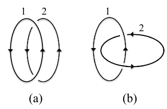
Figure 1: Configurations of (a) zero linking number and (b) nonzero linking number of magnetic and vortex lines.

According to the conservation law in Eq. (34), $Q_{\rm chi}$ alone is not conserved, but what is conserved is the combination $Q_{\rm tot}$ in Eq. (35). This implies that $Q_{\rm chi}$ could be converted to $Q_{\rm mag}$, $Q_{\rm flu}$, and $Q_{\rm mix}$ by the hydrodynamic evolutions Avdoshkin:2014gpa . However, so far, only the physical mechanism that converts $Q_{\rm chi}$ to $Q_{\rm mag}$ is known as the CPI Joyce:1997uy ; Boyarsky:2011uy ; Akamatsu:2013pjd ; Akamatsu:2014yza . If physical processes for other helicity conversions really exist, it follows that, even for neutral chiral plasmas like neutrino gases, where $Q_{\rm mag}$ and $Q_{\rm mix}$ are absent, $Q_{\rm chi}$ can be converted to $Q_{\rm flu}$.

In the following, we explicitly show how the transfer from $Q_{\rm chi}$ to $Q_{\rm flu}$ can occur in the chiral hydrodynamics for neutrinos.

IV Neutrino hydrodynamics

Let us now consider the hydrodynamic regime of the neutrino gas at high density and/or temperature. Although neutrinos interact only very weakly with other particles and the mean free path of neutrinos, $l_{\rm mfp}$, is quite large in typical environments, one can consider the dynamics of the system at the length scale $L\gg l_{\rm mfp}$. In this regime, the neutrino medium can be described by the neutral chiral hydrodynamics. As we will review in Sec. VI.1, the matter density in core-collapse supernovae is so high (and $l_{\rm mfp}$ becomes so small) that the hydrodynamic description for neutrino gases is valid for a rather small length scale compared with astrophysical scales.

For the dense neutrino gas that does not couple to electromagnetic fields, the hydrodynamic equation (III.1) is

$$(\epsilon+P)(\partial_{t}+{\bm{v}}\cdot{\bm{\nabla}}){\bm{v}}=-{\bm{\nabla}}P+\nu{\bm{\nabla}}^{2}{\bm{v}}.$$ (37)

The current conservation is given by

$$\partial_{t}(n+\xi{\bm{v}}\cdot{\bm{\omega}})+{\bm{\nabla}}\cdot{\bm{j}}=0,\qquad{\bm{j}}=n{\bm{v}}+\xi{\bm{\omega}},$$ (38)

where $n$ is the neutrino density. (In this section, we suppress the index $\nu$ that stands for neutrinos for simplicity.) Note that the hydrodynamic equation (37) is the same as the usual one for neutral plasmas, but the current conservation law and the current in Eq. (38) have the corrections due to the CVE.

IV.1 Conservation law of helicity

In the neutrino hydrodynamics, the conservation of helicity is obtained by eliminating the electromagnetic fields in Eq. (34) as

$$\frac{d}{dt}\left(Q+\xi Q_{\rm flu}\right)=0\,,$$ (39)

where $Q$ is the total neutrino number. Note that the total neutrino number $Q$ itself is not conserved.

Usually, one might expect that $Q$ must be conserved, but this is not necessarily the case when one takes into account the quantum effects. The well-known example is the baryon and lepton number violations by the quantum anomalies in the standard model (see, e.g., Ref. Schwartz ). The nonconservation of $Q$ here is a consequence of the mixed gauge-gravitational anomaly in the hydrodynamics regime that appears even in a flat spacetime without gauge fields Landsteiner:2011cp ; Landsteiner:2012kd ; Golkar:2012kb ; Jensen:2012kj .

IV.2 Neutrino-induced fluid helicity (from $Q$ to $Q_{\rm flu}$)

Here we illustrate how the fluid helicity can be generated in the neutrino chiral hydrodynamics in a simple setup. With keeping the application to neutrino gases in core-collapse supernovae in mind, we assume that $\mu\gg T$. Using the thermodynamic relation, $\epsilon+P=\mu n+Ts\simeq\mu n$, the transport coefficient $\xi$ in Eq. (23) reduces to

$$\xi\simeq-\frac{\mu^{2}}{24\pi^{2}}\,,$$ (40)

where we used $C=-1/(4\pi^{2})$ for left-handed neutrinos.

As shown in Fig. 2, we consider an infinitesimal cubic volume element $\Delta V=\Delta x\Delta y\Delta z$ in a vorticity in the positive $z$ direction, ${\bm{\omega}}=\omega\hat{\bm{z}}$. (Note that there is no fluid velocity ${\bm{v}}$ in the $z$ direction in this volume element at the beginning.) In general, the neutrino chemical potential depends on the position, $\mu({\bm{x}})$, and the chemical potential inside this volume element can be slightly different from that outside this region. We denote this difference by $\Delta\mu\equiv\mu_{\rm in}-\mu_{\rm out}$. Assuming $\Delta\mu>0$, the magnitude of the transport coefficient $\xi$ in Eq. (40) is larger inside the volume element by

$$|\Delta\xi|\simeq\frac{\mu}{12\pi^{2}}\Delta\mu\,,$$ (41)

to the order of $O(\Delta\mu)$, where $\mu\equiv\mu_{\rm out}$. Because of the difference $\Delta\xi$ between the inside and the outside, there is an additional chiral vortical current in the negative $z$ direction,

$$\Delta j^{z}_{\rm CVE}=-\frac{\mu\omega}{12\pi^{2}}\Delta\mu\,.$$ (42)

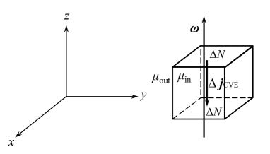
Figure 2: Generation of $Q_{\rm flu}$ in the neutrino hydrodynamics in a vorticity ${\bm{\omega}}$. See the text for further detail.

After an infinitesimally small time interval $\Delta t$, this additional current leads to the accumulation of neutrinos in the lower plane and the depletion in the upper plane, whose number is expressed by $\Delta N=|\Delta j^{z}_{\rm CVE}|\Delta S\Delta t$ with $\Delta S=\Delta x\Delta y$. The difference of neutrino numbers between the upper and lower planes generates the gradient of the pressure, $\partial_{z}P(z)<0$, in the $z$ direction in this volume element. From the hydrodynamic equation (37), this gives rise to the local fluid velocity in the positive $z$ direction,

$$\Delta v_{z}=-\frac{\partial_{z}P}{\epsilon+P}\Delta t\,,$$ (43)

to the order of $O(v)$. As a result of this process, the nonzero fluid helicity is generated in this volume element as

$$\Delta Q_{\rm flu}=\omega\Delta v_{z}\Delta V.$$ (44)

The variations of the neutrino density and/or temperature and the local vorticity can occur in every part of the system, and generates a global fluid helicity $Q_{\rm flu}$ in total. Then, according to Eq. (39), the total neutrino number $Q$ also changes so that the total helicity of the system is conserved. Note here that the parity-violating transport (CVE) is essential to generate the parity-odd $Q_{\rm flu}$; this process is specific for the neutrino chiral hydrodynamics, and it does not occur in the usual hydrodynamics.

V Helical magnetohydrodynamics

We now consider a plasma which includes not only hot and/or dense neutrinos, but also charged electrons. We assume that the momentum exchange between neutrinos and electrons is sufficiently rapid, so that the fluid dynamics is described by the single fluid velocity ${\bm{v}}$ in the hydrodynamic regime of the system. Since the fluid helicity can be generated through the CVE for neutrinos as we have seen above, the system of interest is described by the MHD with finite fluid helicity—helical magnetohydrodynamics.

For simplicity, we assume that the chiral chemical potential for electrons, $\mu_{5}\equiv({\mu_{\rm R}}-{\mu_{\rm L}})/2$, is much smaller than the vector chemical potential, $\mu_{e}\equiv({\mu_{\rm R}}+{\mu_{\rm L}})/2$. (The extension of the following discussion to large $\mu_{5}$ should be straightforward.)

Taking the summation and subtraction of Eq. (34) for right- and left-handed fermions (electrons and neutrinos), we obtain the following relations concerning $Q\equiv Q_{e}^{\rm R}+Q_{e}^{\rm L}+Q_{\nu}^{\rm L}$ and $Q_{5}\equiv Q_{e}^{\rm R}-Q_{e}^{\rm L}-Q_{\nu}^{\rm L}$:

$$\frac{d}{dt}Q =-\frac{d}{dt}(\xi_{\nu}Q_{\rm flu})\,,$$ (45)

$$\frac{d}{dt}\tilde{Q}_{5} =0\,,$$ (46)

where

$$\tilde{Q}_{5}\equiv Q_{5}+\frac{1}{4\pi^{2}}Q_{\rm mag}+(\xi_{e}-\xi_{\nu})Q_{\rm flu}+\xi_{e}^{B}Q_{\rm mix}\,,$$ (47)

with

$$\xi_{e}=\frac{\mu_{e}^{2}}{4\pi^{2}}\left(1-\frac{1}{3}\frac{n_{e}\mu_{e}}{\epsilon+P}\right)+\frac{T^{2}}{12}\left(1-\frac{n_{e}\mu_{e}}{\epsilon+P}\right)\,,$$ (48)

$$\xi_{\nu}=-\frac{\mu_{\nu}^{2}}{8\pi^{2}}\left(1-\frac{2}{3}\frac{n_{\nu}\mu_{\nu}}{\epsilon+P}\right)-\frac{T^{2}}{24}\left(1-\frac{2n_{\nu}\mu_{\nu}}{\epsilon+P}\right)\,,$$ (49)

$$\xi_{e}^{B}=\frac{\mu_{e}}{2\pi^{2}}\left(1-\frac{1}{4}\frac{n_{e}\mu_{e}}{\epsilon+P}\right)-\frac{1}{24}\frac{n_{e}T^{2}}{\epsilon+P}\,.$$ (50)

Equations (45) and (46) represent the violation of the lepton number and the conservation of total helicity, respectively. Both the violation of the lepton number and the modifications of the axial charge originate from the quantum anomalies in the hydrodynamic regime. Note that, even for finite $\nu$ and $\eta$, the contribution of the dissipative terms to these relations is negligibly small when $\mu_{5}\ll\mu_{e},T$.

V.1 Helical magnetic effect

When the nonzero global fluid helicity $Q_{\rm flu}$ is generated from the neutrino medium, it necessarily implies a nonvanishing local fluid helicity $n_{\rm flu}({\bm{x}})\equiv{\bm{v}}\cdot{\bm{\omega}}$ in some region. Then, $n_{\rm flu}$ effectively acts as a chiral chemical potential $\mu_{5}$ for the other charged particles. In fact, $n_{\rm flu}$ has the same mass dimension and the same quantum numbers as $\mu_{5}$, and the following current as a response to $n_{\rm flu}$ and ${\bm{B}}$ is generally allowed to emerge in terms of ${\cal C}$, ${\cal P}$, and ${\cal T}$ symmetries:

$${\bm{j}}_{\rm HME}=\kappa_{B}n_{\rm flu}{\bm{B}}.$$ (51)

Compared with the expression of the CME for Dirac particles, ${\bm{j}_{\rm CME}}\propto\mu_{5}{\bm{B}}$ Vilenkin:1980fu ; Nielsen:1983rb ; Alekseev:1998ds ; Fukushima:2008xe , the coefficient $\mu_{5}$ is replaced by $n_{\rm flu}$ with some proportionality constant $\kappa_{B}$ of order $1$. We refer to it as the “helical magnetic effect” (HME).

A similar effect is known as the $\alpha$-effect in plasma physics Davidson , where $\langle n_{\rm flu}({\bm{x}})\rangle$ with the mean value averaged over the turbulent fluctuations is considered to arise by helical turbulence. However, it is not clear, as a matter of principle, how a parity-odd fluid helicity can be created globally (i.e., $Q_{\rm flu}=\int d^{3}{\bm{x}}\langle n_{\rm flu}\rangle\neq 0$) in the evolutions of conventional parity-preserving hydrodynamic equations. In contrast, in our argument, the parity symmetry is broken by the chirality of neutrinos and the global fluid helicity can be generated naturally.

V.2 Helical plasma instability (from $Q_{\rm flu}$ to $Q_{\rm mag}$)

When electromagnetic fields evolve dynamically in the presence of the HME in Eq. (51), an instability similar to the CPI develops. (For the physical picture of the CPI, see Ref. Akamatsu:2014yza .) We will call it the “helical plasma instability” (HPI). Here we provide a derivation of the HPI in an analytically tractable setup.

We consider the region where $n_{\rm flu}({\bm{x}})\neq 0$ and $n_{\rm mix}({\bm{x}})=0$, and assume that the variation of the fluid helicity is much smaller than its magnitude, $|{\bm{\nabla}}n_{\rm flu}/n_{\rm flu}|\ll|n_{\rm flu}|$. The equation for ${\bm{B}}$ is obtained by replacing the chiral magnetic current $\xi_{B}{\bm{B}}$ by the helical magnetic current $\kappa_{B}n_{\rm flu}{\bm{B}}$ and by turning off the chiral vortical current $\xi{\bm{\omega}}$ in Eq. (III.2) as

$$\partial_{t}{\bm{B}}={\bm{\nabla}}\times({\bm{v}}\times{\bm{B}})+\eta({\bm{\nabla}}^{2}{\bm{B}}+\kappa_{B}n_{\rm flu}{\bm{\nabla}}\times{\bm{B}}).$$ (52)

Here we concentrated on the magnetic field with the momentum $k\sim n_{\rm flu}$, and dropped the term ${\bm{\nabla}}n_{\rm flu}\times{\bm{B}}$. As we will show in Eq. (55) below, the typical momentum scale of the HPI is actually the magnitude of the local fluid helicity $n_{\rm flu}$.

Equation (52) has unstable modes. To see this, we take $v_{x}=v_{y}=0$, $v_{z}\neq 0$ with $\partial_{y}v_{x}=-\partial_{x}v_{y}\neq 0$ (and we set all the other components zero) so that $n_{\rm flu}=v_{z}\omega_{z}\neq 0$ in this region. We consider a perturbation of the magnetic field of the form,

$${\bm{B}}_{\pm}=({\bm{e}}_{x}\pm i{\bm{e}}_{y})e^{-i\omega t+ikz},$$ (53)

where the subscript $\pm$ denotes the state with helicity $\pm 1$ for positive $k$. Substituting it into Eq. (52), we get the dispersion relation,

$$\omega=\mp\partial_{y}v_{x}+kv_{z}-i\eta k(k\mp\kappa_{B}n_{\rm flu}).$$ (54)

The imaginary part of $\omega$ becomes maximal when

$$k_{\rm inst}=\pm\kappa_{B}n_{\rm flu}/2,$$ (55)

for which $\omega$ has the positive imaginary part. At $k=k_{\rm inst}$, the magnetic field grows exponentially (at least initially) as

$$|B(t)|=|B(0)|e^{\eta(\kappa_{B}n_{\rm flu})^{2}t/4}.$$ (56)

This is the HPI. The resulting magnetic field acquires a nonzero magnetic helicity, similarly to the CPI Joyce:1997uy ; Boyarsky:2011uy ; Akamatsu:2013pjd ; Akamatsu:2014yza . In the present case, however, the change of the magnetic helicity is accompanied by the change of the fluid helicity due to the conservation of total helicity [see Eqs. (46) and (47)], but not that of $\mu_{5}$ as in Refs. Joyce:1997uy ; Boyarsky:2011uy ; Akamatsu:2013pjd ; Akamatsu:2014yza .

V.3 Helical vortical effect

As we will see in Sec. V.4, the fluid helicity $Q_{\rm flu}$ can also be converted to the cross helicity $Q_{\rm mix}$ by the helical hydrodynamic evolution. Here, notice that the local cross helicity $n_{\rm mix}={\bm{v}}\cdot{\bm{B}}$ has the same mass dimension and the same quantum numbers as $\mu_{e}\mu_{5}$ (but not $\mu_{5}$ itself). Hence, similarly to the CVE for Dirac particles, ${\bm{j}}_{\rm CVE}\propto\mu_{e}\mu_{5}{\bm{\omega}}$ Vilenkin:1979ui ; Son:2009tf ; Landsteiner:2011cp , $n_{\rm mix}$ can induce a current in a vorticity,

$${\bm{j}}_{\rm HVE}=\kappa n_{\rm mix}{\bm{\omega}},$$ (57)

with some constant $\kappa$ of order $1$. We call it as the “helical vortical effect” (HVE).

One might expect that ${\bm{j}}\sim n_{\rm mag}{\bm{B}}$, with $n_{\rm mag}={\bm{A}}\cdot{\bm{B}}$ being the local “magnetic helicity,” should exist as well, since this relation is consistent with ${\cal C}$, ${\cal P}$, and ${\cal T}$ symmetries. However, $n_{\rm mag}$ is not gauge invariant and does not make sense locally, unlike the global magnetic helicity $Q_{\rm mag}$ which is gauge invariant under the appropriate boundary conditions (e.g., ${\bm{B}}\rightarrow{\bm{0}}$ at infinity). Therefore, we do not consider the current of the form ${\bm{j}}\sim n_{\rm mag}{\bm{B}}$.

V.4 From $Q_{\rm flu}$ to $Q_{\rm mix}$ and vice versa

We now show, from the argument parallel to the one in Sec. IV.2, that the cross helicity $Q_{\rm mix}$ can be generated from the fluid helicity $Q_{\rm flu}$ through the HME, and that $Q_{\rm flu}$ can be generated from $Q_{\rm mix}$ through the HVE. For the later purpose, we set $\alpha\equiv\kappa_{B}n_{\rm flu}$ and $\beta\equiv\kappa n_{\rm mix}$.

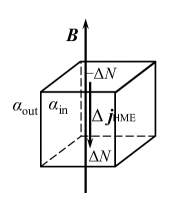
Figure 3: Generation of $Q_{\rm mix}$ from $Q_{\rm flu}$ in the MHD. See the text for further detail.

We consider an infinitesimal cubic volume element $\Delta V$ in a magnetic field, ${\bm{B}}=B\hat{\bm{z}}$, as shown in Fig. 3. We assume that $\alpha_{\rm in}$ inside this volume element is smaller than $\alpha_{\rm out}$ outside the region, and we denote this difference by $\Delta\alpha\equiv\alpha_{\rm in}-\alpha_{\rm out}<0$. This difference leads to an additional helical magnetic current in the negative $z$ direction,

$$\Delta j^{z}_{\rm HME}=B\Delta\alpha.$$ (58)

After a time $\Delta t$, this additional current leads to the increase of the charged particles in the lower plane by $\Delta N=\Delta j^{z}_{\rm HME}\Delta S\Delta t$ and the decrease in the upper plane by $\Delta N$. Analogously to Eq. (43), this yields $v_{z}>0$, and consequently, the nonzero cross helicity is generated in this volume element as

$$\Delta Q_{\rm mix}=B\Delta v_{z}\Delta V.$$ (59)

Note that the presence of $Q_{\rm flu}$ is essential in this process to produce $Q_{\rm mix}$.

The generation of $Q_{\rm flu}$ from $Q_{\rm mix}$ can be understood in a similar manner. With $\Delta\beta\equiv\beta_{\rm in}-\beta_{\rm out}<0$ in a vorticity ${\bm{\omega}}=\omega\hat{\bm{z}}$, we have the additional helical cortical current in the volume element,

$$\Delta j^{z}_{\rm HVE}=\omega\Delta\beta.$$ (60)

This current leads to $v_{z}>0$, which then provides the nonzero fluid helicity,

$$\Delta Q_{\rm flu}=\omega\Delta v_{z}\Delta V.$$ (61)

V.5 Towards saturation

We have seen above that different types of helicity can be converted to each other by the evolutions in helical MHD: conversion from $Q_{\rm flu}$ to $Q_{\rm mix}$ and $Q_{\rm mag}$, and conversion from $Q_{\rm mix}$ to $Q_{\rm flu}$ and $Q_{\rm mag}$. (Here conversion from $Q_{\rm mix}$ to $Q_{\rm mag}$ occurs, at least, by combining two processes from $Q_{\rm mix}$ to $Q_{\rm flu}$ and from $Q_{\rm flu}$ to $Q_{\rm mag}$.)

We note that our argument here provides an explicit realization of the possible new “instability” suggested in Ref. Avdoshkin:2014gpa . This is a kind of extension of the CPI in kinetic theory Akamatsu:2013pjd to the hydrodynamic regime, where chiral charge of fermions is transferred not only to $Q_{\rm mag}$, but also to $Q_{\rm flu}$ and $Q_{\rm mix}$. As far as we know, however, we do not find any exponentially growing mode concerning the helicity conversion from the chiral charge to $Q_{\rm flu}$ and $Q_{\rm mix}$ unlike the CPI Joyce:1997uy ; Boyarsky:2011uy ; Akamatsu:2013pjd ; Akamatsu:2014yza or HPI. So we regard this mechanism as a “helicity transmutation” rather than the “instability” at this moment.

How the system saturates after the helicity transmutation depends on the details of the system, and its quantitative understanding requires 3D helical MHD simulations with the appropriate initial conditions. It is plausible to expect that, if the conversion efficiency of the helicity is sufficient, the magnitude of each term in Eq. (47) should be of the same order after the saturation.

VI Application to core-collapse supernovae

We now apply our mechanism above to core-collapse supernovae, where left-handed neutrinos are abundantly produced by the electron capture $p+e^{-}\rightarrow n+\nu_{e}$ and form a Fermi degenerate matter Kotake:2005zn ; Shapiro . The key point that has not been appreciated so far, to our knowledge, is that the neutrino matter here is a chiral liquid. Below we will concentrate on electron neutrinos (which we will denote as $\nu$), since only they are numerously generated in this process during the core collapse. To illustrate the new chiral effects of neutrinos, we ignore the general relativistic corrections.

VI.1 Applicability of neutrino hydrodynamics

Let us first discuss the applicability of the neutrino hydrodynamics at the core of the supernova. For this purpose, recall the expression for the mean free path of neutrinos due to the coherent scattering with nuclei Kotake:2005zn ,

$$l_{\rm mfp}\sim 10^{7}\ {\rm cm}\left(\frac{\rho}{10^{10}\ {\rm g}/{\rm cm}^{3}}\right)^{\!-\frac{5}{3}}\left(\frac{A}{56}\right)^{\!-1}\left(\frac{Y_{e}}{26/56}\right)^{\!-\frac{2}{3}}\,,$$

where $\rho$ is the mass density of nuclear matter, $A$ is the atomic mass number, and $Y_{e}$ is the electron fraction. Equation (VI.1) can be understood from the expression of the mean free path, $l_{\rm mfp}=(\sigma_{A}n_{A})^{-1}$, where $\sigma_{A}$ is the cross section and $n_{A}$ is the number density of nuclei. By using $\sigma_{A}\sim G_{\rm F}^{2}E_{\nu}^{2}A^{2}$ Tubbs:1975jx and $n_{A}=\rho/(Am_{N})$, where $G_{\rm F}$ is the Fermi constant, $E_{\nu}\simeq\mu_{e}=(3\pi^{2}\rho Y_{e}/m_{N})^{1/3}$ is the neutrino energy, and $m_{N}$ is the nucleon mass, one arrives at Eq. (VI.1).

Substituting the typical magnitudes of the quantities appearing in Eq. (VI.1) at the core, $\rho\gtrsim 10^{13}\ {\rm g}/{\rm cm}^{3}$, $A\simeq 56$, and $Y_{e}\sim 0.1$, we have $l_{\rm mfp}\lesssim 1\ {\rm m}$. (For the highest density $\rho\sim 10^{15}\ {\rm g}/{\rm cm}^{3}$, we have even $l_{\rm mfp}\sim 1\ {\rm cm}$.) Therefore, the hydrodynamic description for dense neutrino gases should be valid at the astrophysical length scale $L\gg l_{\rm mfp}$, at least at the core of the supernova. (Recall that the typical radius of the core is of order $100$ km.) In the lower density region where hydrodynamics for neutrinos becomes invalid, one needs to use the chiral kinetic theory for neutrino gases instead (see Sec. II), which is beyond the scope of the present paper.

VI.2 Estimate of magnetic fields

From now on, we provide a simple estimate of the maximum magnetic field that can be generated by our mechanism. Our estimate below should be regarded as schematic.

The highest temperature is $T\sim 10$ MeV and the maximum neutrino and electron chemical potentials at the core are on the order of the nuclear scale, $\mu_{\nu}\sim\mu_{e}\sim\Lambda$, where $\Lambda\equiv 200$ MeV. The latter fact may be understood from the near $\beta$ equilibrium condition, charge neutrality, and the typical lepton fraction: $\mu_{n}+\mu_{\nu}\simeq\mu_{p}+\mu_{e}$, $n_{p}=n_{e}$, and $Y_{l}\equiv(n_{e}+n_{\nu})/(n_{n}+n_{p})\sim 0.1$. Here $\mu_{n}$ and $\mu_{p}$ are the neutron and proton chemical potentials, and $n_{n}$ and $n_{p}$ are the neutron and proton densities, all of which are set by the nuclear scale.

As the time scale of the core collapse, $t_{\rm coll}\sim 1$ s, is much larger than the time scale corresponding to the typical energy scale in the chiral hydrodynamics, $\Lambda^{-1}\sim 10^{-23}$ s, there must be sufficient time for the saturation of the helicity transmutation to be achieved. Hence, assuming the sufficient conversion efficiency of the helicity, we expect that (see Sec. V.5)

$$Q_{\rm mag}\sim\mu_{\nu}^{2}Q_{\rm flu}\sim Q_{\nu}^{0}\sim V\Lambda^{3},$$ (63)

after the saturation for $\mu_{\nu}\gg T$, where $Q_{\nu}^{0}$ is the initial neutrino number at the core and $V$ is the volume of the core. Then, the typical magnitude of the local fluid helicity $n_{\rm flu}\sim Q_{\rm flu}/V$ is of order $\Lambda$, and so is the typical momentum scale of the HPI from Eq. (55), $k_{\rm inst}\sim\Lambda$. Considering $Q_{\rm mag}\sim VB_{\rm core}^{2}/k_{\rm inst}$, we obtain

$$B_{\rm core}\sim\Lambda^{2}\sim 10^{18}\ {\rm Gauss}.$$ (64)

Hence, the maximum magnetic field generated by this mechanism is set by the nuclear scale.

VI.3 Discussion

Finally, we discuss several important effects concerning our mechanism that we have ignored so far.

VI.3.1 Helical turbulence and inverse cascade

At first sight, the typical length scale of the magnetic field, $k_{\rm inst}^{-1}\sim\Lambda^{-1}\sim 10^{-15}\ {\rm m}$, generated just after the HPI is too small compared with astrophysical scales. Yet, there exists a mechanism, called the inverse cascade, that enhances a wavelength of a magnetic field to a macroscopic length scale by a MHD turbulence Biskamp . The inverse cascade is known to take place in charged plasmas with nonzero magnetic helicity Biskamp , which is the case for electromagnetic plasmas coupled with neutrinos in Sec. V. The possible inverse cascade in the 3D helical MHD also gives rise to a large-scale coherent fluid motion, which is favorable for the supernova explosion itself. This should be contrasted with the direct cascade observed in the conventional 3D neutrino-radiation hydrodynamics that tends to make the explosion rather difficult Hanke:2011jf . To what extent the inverse cascade is efficient in the present case should be checked in the future 3D helical MHD simulations.

VI.3.2 Chirality flipping

We then consider the effects of chirality flipping by fermion masses. Since chirality flipping from left-handed neutrinos to right-handed ones is negligible, the generation of fluid helicity in the neutrino hydrodynamics in Sec. IV.2 should not be prevented by the fermion mass. On the other hand, chirality flipping by the electron mass can decrease the chiral charge of electrons, $Q_{5}$, even if it is generated in the weak process Ohnishi:2014uea or by the inverse process from $Q_{\rm mag}$, $Q_{\rm flu}$, or $Q_{\rm mix}$. Although such an inverse process is generally allowed, we expect it to cease after the saturation of the helicity transmutation, as we argued in Sec. V.5. Then, $Q_{\rm mag}$, $Q_{\rm flu}$, and $Q_{\rm mix}$, which are not affected by the nonzero electron mass, remain nonzero after the saturation, while $Q_{5}$ is damped. The resulting $Q_{\rm mag}$, $Q_{\rm flu}$, and $Q_{\rm mix}$ can play important roles in the subsequent evolutions of the stars and, especially, $Q_{\rm mag}$ possibly accounts for the origin of magnetars. Whether this expectation is correct or not needs to be tested in the helical MHD simulations as well.

VI.3.3 Profiles of proto-neutron stars

One might wonder if all the newly born neutron stars just after supernova explosions become magnetars by this mechanism. Note that our estimate here provides a maximum magnetic field assuming the sufficient conversion efficiency of the helicity of neutrinos into that of electromagnetic fields. To clarify this point, it is also important to understand the realistic conversion efficiency that should depend on individual profiles of proto-neutron stars, such as the initial rotation and magnetic field.

VII Outlook

In this paper, we pointed out that the chirality (or the left-handedness) of neutrinos leads to a number of new phenomenological consequences in a hot and dense neutrino medium and charged plasmas coupled with it. In particular, we found that the neutrino density can be converted to the fluid helicity of the neutrino medium. The resulting fluid helicity effectively acts as a chiral chemical potential for other charged particles, and induces various helical effects, such as the helical magnetic effect, helical vortical effect, and helical plasma instability. Through these helical effects, the fluid helicity can also be converted to the magnetic helicity and cross helicity.

In the context of core-collapse supernovae, this provides a new mechanism for converting the gravitational energy released by the core collapse to the fluid energy and the electromagnetic energy, which may explain the possible origin of magnetars. Since our mechanism modifies the structure and evolution of the fluid motion and those of electromagnetic fields, this is relevant to the question of the supernova explosion itself.

There are several future directions of our work. Among others, our new mechanism should be numerically checked in the 3D chiral neutrino-radiation hydrodynamics. It would be important to see if and how the conventional picture of the supernova explosion is modified quantitatively or even qualitatively. It would also be interesting to study the possible impacts of new collective modes specific for neutrino gases due to the chiral effects, such as the analogue of the chiral Alfvén wave in a rotation Yamamoto:2015ria , chiral vortical wave Jiang:2015cva , and chiral heat wave Chernodub:2015gxa .

Our primary interest in this paper has been focused on the dense neutrino medium in core-collapse supernovae. However, the mechanism of the helicity transmutation itself is general and is applicable to other chiral matter as well, such as the electroweak plasma in the early Universe Joyce:1997uy ; Boyarsky:2011uy , quark-gluon plasmas created in heavy ion collisions Kharzeev:2007jp ; Fukushima:2008xe (see also Ref. Kharzeev:2015znc for a recent review), and Weyl semimetals Vishwanath ; BurkovBalents ; Xu-chern . One may also consider the possible generation of lepton number from the fluid helicity in the cosmology. We defer these questions to future work.

- (1) K. Kotake, K. Sato, and K. Takahashi, Rept. Prog. Phys. 69, 971 (2006).
- (2) H. T. Janka, Ann. Rev. Nucl. Part. Sci. 62, 407 (2012).
- (3) T. Takiwaki, K. Kotake, and Y. Suwa, Astrophys. J. 786, 83 (2014).
- (4) T. Melson, H. T. Janka, and A. Marek, Astrophys. J. 801, L24 (2015).
- (5) B. Müller, Mon. Not. Roy. Astron. Soc. 453, 287 (2015).
- (6) D. T. Son and N. Yamamoto, Phys. Rev. Lett. 109, 181602 (2012).
- (7) M. A. Stephanov and Y. Yin, Phys. Rev. Lett. 109, 162001 (2012).
- (8) D. T. Son and N. Yamamoto, Phys. Rev. D 87, 085016 (2013).
- (9) J.-W. Chen, S. Pu, Q. Wang, and X.-N. Wang, Phys. Rev. Lett. 110, 262301 (2013).
- (10) C. Manuel and J. M. Torres-Rincon, Phys. Rev. D 89, 096002 (2014).
- (11) C. Manuel and J. M. Torres-Rincon, Phys. Rev. D 90, 076007 (2014).
- (12) J. Y. Chen, D. T. Son, M. A. Stephanov, H. U. Yee, and Y. Yin, Phys. Rev. Lett. 113, 182302 (2014).
- (13) J. Y. Chen, D. T. Son, and M. A. Stephanov, Phys. Rev. Lett. 115, 021601 (2015).
- (14) D. T. Son and P. Surówka, Phys. Rev. Lett. 103, 191601 (2009).
- (15) S. Adler, Phys. Rev. 177, 2426 (1969).
- (16) J. S. Bell and R. Jackiw, Nuovo Cimento 60A, 47 (1969).
- (17) A. Vilenkin, Phys. Rev. D 22, 3080 (1980).
- (18) H. B. Nielsen and M. Ninomiya, Phys. Lett. B 130, 389 (1983).
- (19) A. Y. Alekseev, V. V. Cheianov, and J. Frohlich, Phys. Rev. Lett. 81, 3503 (1998).
- (20) K. Fukushima, D. E. Kharzeev, and H. J. Warringa, Phys. Rev. D 78, 074033 (2008).
- (21) A. Vilenkin, Phys. Rev. D 20, 1807 (1979).
- (22) K. Landsteiner, E. Megias, and F. Pena-Benitez, Phys. Rev. Lett. 107, 021601 (2011).
- (23) K. Landsteiner, E. Megias, and F. Pena-Benitez, Lect. Notes Phys. 871, 433 (2013).
- (24) A. Ohnishi and N. Yamamoto, arXiv:1402.4760 [astro-ph.HE].
- (25) G. Sigl and N. Leite, JCAP 1601, 025 (2016).
- (26) J. Charbonneau and A. Zhitnitsky, JCAP 1008, 010 (2010).
- (27) M. Kaminski, C. F. Uhlemann, M. Bleicher, and J. Schaffner-Bielich, arXiv:1410.3833 [nucl-th].
- (28) E. Shaverin and A. Yarom, arXiv:1411.5581 [hep-th].
- (29) Y. Akamatsu and N. Yamamoto, Phys. Rev. Lett. 111, 052002 (2013).
- (30) Y. Akamatsu and N. Yamamoto, Phys. Rev. D 90, 125031 (2014).
- (31) M. Joyce and M. E. Shaposhnikov, Phys. Rev. Lett. 79, 1193 (1997).
- (32) A. Boyarsky, J. Frohlich, and O. Ruchayskiy, Phys. Rev. Lett. 108, 031301 (2012).
- (33) R. C. Duncun and C. Thompson, Astrophys. J. 392, L9 (1992).
- (34) D. Grabowska, D. B. Kaplan, and S. Reddy, Phys. Rev. D 91, 085035 (2015).
- (35) A. K. Harding and D. Lai, Rept. Prog. Phys. 69, 2631 (2006).
- (36) H. C. Spruit, AIP Conf. Proc. 983, 391 (2008).
- (37) D. H. Brownell and J. Callaway, Nuovo Cimento B 60, 169 (1969).
- (38) M. J. Rice, Phys. Lett. A 29, 637 (1969).
- (39) S. D. Silverstein, Phys. Rev. Lett. 23,139 (1969); Phys. Rev. Lett. 23, 453(E) (1969).
- (40) K. Makishima, Prog. Theor. Phys. Suppl. 151, 54 (2003).
- (41) T. Tatsumi, Phys. Lett. B 489, 280 (2000).
- (42) D. T. Son and M. A. Stephanov, Phys. Rev. D 77, 014021 (2008).
- (43) M. Eto, K. Hashimoto, and T. Hatsuda, Phys. Rev. D 88, 081701 (2013).
- (44) S. W. Bruenn, Astrophys. J. Suppl. 58, 771 (1985).
- (45) M. V. Berry, Proc. R. Soc. Lond. A 392, 45 (1984).
- (46) G. E. Volovik, The Universe in a Helium Droplet (Clarendon Press, Oxford, 2003).
- (47) G. Sundaram and Q. Niu, Phys. Rev. B 59, 14915 (1999).
- (48) D. Xiao, J. Shi, and Q. Niu, Phys. Rev. Lett. 95, 137204 (2005).
- (49) C. Duval, Z. Horváth, P. A. Horváthy, L. Martina, and P. Stichel, Mod. Phys. Lett. B 20, 373 (2006).
- (50) J. Erdmenger, M. Haack, M. Kaminski, and A. Yarom, JHEP 0901, 055 (2009).
- (51) N. Banerjee, J. Bhattacharya, S. Bhattacharyya, S. Dutta, R. Loganayagam, and P. Surówka, JHEP 1101, 094 (2011).
- (52) Y. Neiman and Y. Oz, JHEP 1103, 023 (2011).
- (53) S. Golkar and D. T. Son, JHEP 1502, 169 (2015).
- (54) K. Jensen, R. Loganayagam, and A. Yarom, JHEP 1302, 088 (2013).
- (55) R. Loganayagam and P. Surówka, JHEP 1204, 097 (2012).
- (56) J. H. Gao, Z. T. Liang, S. Pu, Q. Wang, and X. N. Wang, Phys. Rev. Lett. 109, 232301 (2012).
- (57) L. D. Landau and E. M. Lifshitz, Fluid Mechanics (Pergamon, New York, 1959).
- (58) Y. Minami and Y. Hidaka, Phys. Rev. E 87, 023007 (2013).
- (59) M. Liebendoerfer, M. Rampp, H.-T. Janka, and A. Mezzacappa, Astrophys. J. 620, 840 (2005).
- (60) R. Buras, H. T. Janka, M. Rampp, and K. Kifonidis, Astron. Astrophys. 457, 281 (2006).
- (61) P. A. Davidson, An Introduction to Magnetohydrodynamics (Cambridge University Press, Cambridge, England, 2001).
- (62) A. Avdoshkin, V. P. Kirilin, A. V. Sadofyev, and V. I. Zakharov, arXiv:1402.3587 [hep-th].
- (63) M. D. Schwartz, Quantum Field Theory and the Standard Model (Cambridge University Press, Cambridge, England, 2013).
- (64) S. L. Shapiro and S. A. Teukolsky, Black Holes, White Dwarfs, and Neutron Stars (Wiley, New York, 1983).
- (65) D. L. Tubbs and D. N. Schramm, Astrophys. J. 201, 467 (1975).
- (66) L. F. Roberts, Astrophys. J. 755, 126 (2012).
- (67) See, e.g., D. Biskamp, Nonlinear Magnetohydrodynamics (Cambridge University Press, Cambridge, England, 1993).
- (68) N. Yamamoto, in preparation.
- (69) Y. Hirono, D. Kharzeev, and Y. Yin, Phys. Rev. D 92, 125031 (2015).
- (70) F. Hanke, A. Marek, B. Muller, and H. T. Janka, Astrophys. J. 755, 138 (2012).
- (71) N. Yamamoto, Phys. Rev. Lett. 115, 141601 (2015).
- (72) Y. Jiang, X. G. Huang, and J. Liao, Phys. Rev. D 92, 071501 (2015).
- (73) M. N. Chernodub, arXiv:1509.01245 [hep-th].
- (74) D. E. Kharzeev, L. D. McLerran, and H. J. Warringa, Nucl. Phys. A 803, 227 (2008).
- (75) D. E. Kharzeev, J. Liao, S. A. Voloshin, and G. Wang, arXiv:1511.04050 [hep-ph].
- (76) X. Wan, A. M. Turner, A. Vishwanath, and S. Y. Savrasov, Phys. Rev. B 83, 205101 (2011).
- (77) A. A. Burkov and L. Balents, Phys. Rev. Lett. 107, 127205 (2011).
- (78) G. Xu, H. Weng, Z. Wang, X. Dai, and Z. Fang, Phys. Rev. Lett. 107, 186806 (2011).