Wigner Distributions and Orbital Angular Momentum of Quarks and Gluons

Abstract:

We present a recent calculation of the Wigner distributions of quarks and gluons in a perturbative model. We also present the results for the orbital angular momentum and the spin-orbit correlations.

1 Introduction

Recently the Wigner distributions of quarks and gluons inside the nucleon [1, 2] have been proposed as a tool to access the still unknown orbital angular momentum of quarks and gluons and its contribution to the nucleon spin. The ’nucleon spin problem’ is till now one of the most intriguing problems in hadron physics that has to be understood. It was found in the EMC experiment [3] that the quarks carry about 25 % of the nucleon spin, which suggested that a large fraction of the contributions come from the intrinsic spin of the quarks and gluons and their orbital angular momentum (OAM). There have been tremendous efforts and advances both in theoretical and experimental sides to unravel the different components and contributions to the proton spin. Most recently, a global analysis [4] including high statistics data from STAR and PHENIX collaborations at RHIC, BNL found that the gluon spin contribution may be about 35 % of the proton spin. This result has a lot of uncertainties in the small x region. In any case, quark and gluon OAM play a substantial role in building up the proton spin.

An issue that complicates the understanding of the nucleon spin in terms of its different components is gauge invariance. There are two main decomposition of nucleon spin. In the so-called canonical decomposition [5], one writes the nucleon helicity in terms of the intrinsic quark spin ($\Delta q$), intrinsic gluon spin ($\Delta g$) and quark and gluon OAM ($l_{q/g}$). Except for the quark spin, it has been shown that the other terms depend on the choice of the gauge. In the kinetic decomposition of the nucleon spin [6], one writes the nucleon helicity in terms of the intrinsic quark spin ($\Delta q$), quark OAM ($L^{q}$), and the total contribution of the gluon angular momentum ($J^{g}$). Wakamatsu [7] separated $J^{g}$ in the kinetic decomposition into an orbital part and an intrinsic part using a prescription similar to [8]. The kinetic and canonical OAM differ in the choice of Wilson line needed for the color gauge invariance. A physical interpretation of both types of OAM can be found in [9].

Wigner distributions, which are quasiprobabilistic distributions, are known in the context of quantum mechanics since a long time [10]. Because of Heisenberg uncertainty principle, a quantum phase space description is not possible for observables. Wigner distributions, which are joint position and momentum space distributions do not have probabilistic interpretation. Wigner distributions for the quarks and gluons in the nucleon are 6 dimensional objects, 3 positions and 3 momentum. By integrating out one or more variables, one obtains the reduced Wigner distributions. These can have probabilistic interpretation. Wigner distributions in the light-cone or infinite momentum frame were introduced in [11]. These are related to the generalized parton correlation functions (GPCFs), which are fully unintegrated off-forward parton correlators that contain maximum amount of information on the correlations of quarks and gluons inside the nucleon. Integrating the GPCFs over the light cone energy $k^{-}$ one gets the generalized transverse momentum dependent pdfs (GTMDs) [12]. These GTMDs can be expressed as Fourier transforms of the Wigner distributions. Integrating over more variables, one can connect the Wigner distributions to the generalized parton distribution (GPDs) and transverse momentum dependent distributions (TMDs), both of which are known to give important information on the momentum and angular momentum correlations of the quarks and gluons inside the nucleon. Thus these are called ’mother distributions’ containing maximum information on the internal structure of the nucleons.

Wigner distributions can be related to the OAM of the quarks and gluons as well as their spin-orbit correlations. In this way these can give informations beyond those that can be obtained from TMDs and GPDs. As the Wigner distributions themselves cannot be directly measured experimentally, informations about them can be obtained indirectly through the measurement of other observables. That is why model calculations of Wigner distributions are interesting as these give valuable insight into these objects. Models in which Wigner distributions have been investigated in the literature include constituent quark model and chiral quark soliton model [11]. Both of these are phenomenological models of the nucleon and they do not contain any gluonic degrees of freedom. We present a recent calculation of the Wigner distributions in a perturbative model with a gluonic degree of freedom, namely a quark dressed with a gluon [13, 14]. We use light-front Hamiltonian approach and express the Wigner distributions in terms of overlaps of light-front wave function (LFWFs). The state can be thought of as a spin 1/2 relativistic composite object. This approach gives an intuitive picture of deep inelastic processes; it is based on field theory but at the same time keeps close contact with the parton model ideas [15], the field theoretic partons have intrinsic transverse momenta and they interact. The advantage is that as there are gluonic degrees of freedom it is possible to investigate both quark and gluon Wigner distributions.

2 Wigner distributions for the quarks and gluons

The Wigner distribution of quarks can be defined as the two-dimensional Fourier transforms [11, 12]

$$\rho^{[\Gamma]}({b}_{\perp},{k}_{\perp},x,\sigma)=\int\frac{d^{2}\Delta_{\perp}}{(2\pi)^{2}}e^{-i\Delta_{\perp}.b_{\perp}}W^{[\Gamma]}(\Delta_{\perp},{k}_{\perp},x,\sigma);$$ (1)

where $\Delta_{\perp}$ is momentum transfer of the target in transverse direction and ${b}_{\perp}$ is the impact parameter conjugate to $\Delta_{\perp}$. $W^{[\Gamma]}$ is the quark-quark correlator:

$$W^{[\Gamma]}({\Delta}_{\perp},{k}_{\perp},x,\sigma)=\Big{\langle}p^{+},\frac{\Delta_{\perp}}{2},\sigma\Big{|}W^{[\Gamma]}(0_{\perp},k_{\perp},x)\Big{|}p^{+},-\frac{\Delta_{\perp}}{2},\sigma\Big{\rangle}$$

$$=\frac{1}{2}\int\frac{dz^{-}d^{2}z_{\perp}}{(2\pi)^{3}}e^{i(xp^{+}z^{-}/2-k_{\perp}.z_{\perp})}\Big{\langle}p^{+},\frac{\Delta_{\perp}}{2},\sigma\Big{|}\overline{\psi}(-\frac{z}{2})\Omega\Gamma\psi(\frac{z}{2})\Big{|}p^{+},-\frac{\Delta_{\perp}}{2},\sigma\Big{\rangle}\Big{|}_{z^{+}=0}.$$ (2)

We use the symmetric frame where $p^{+}$ and $\sigma$ define the longitudinal momentum of the target state and its helicity respectively. $x=k^{+}/p^{+}$ is the fraction of longitudinal momentum fraction carried by the active quark. $\Omega$ is the gauge link needed for color gauge invariance. In this work, we use the light-front gauge and take the gauge link to be unity. The symbol $\Gamma$ is the Dirac matrix defining the types of quark densities; we take $\Gamma=\gamma^{+}$ and $\gamma^{+}\gamma^{5}$ respectively.

We denote the different Wigner distributions by $\rho_{\lambda\lambda^{\prime}}$ [11], where $\lambda(\lambda^{\prime})$ is longitudinal polarization of target state(quark).

$$\rho_{UU}({b}_{\perp},{k}_{\perp},x)=\frac{1}{2}\Big{[}\rho^{[\gamma^{+}]}({b}_{\perp},{k}_{\perp},x,+{e}_{z})+\rho^{[\gamma^{+}]}({b}_{\perp},{k}_{\perp},x,-{e}_{z})\Big{]}$$ (3)

gives the Wigner distribution of unpolarized quarks in the unpolarized target state.

$$\rho_{LU}({b}_{\perp},{k}_{\perp},x)=\frac{1}{2}\Big{[}\rho^{[\gamma^{+}]}({b}_{\perp},{k}_{\perp},x,+{e}_{z})-\rho^{[\gamma^{+}]}({b}_{\perp},{k}_{\perp},x,-{e}_{z})\Big{]}$$ (4)

gives the distortion due to the longitudinal polarization of the target state.

$$\rho_{UL}({b}_{\perp},{k}_{\perp},x)=\frac{1}{2}\Big{[}\rho^{[\gamma^{+}\gamma_{5}]}({b}_{\perp},{k}_{\perp},x,+{e}_{z})+\rho^{[\gamma^{+}\gamma_{5}]}({b}_{\perp},{k}_{\perp},x,-{e}_{z})\Big{]}$$ (5)

represents the distortion due to the longitudinal polarization of quarks.

$$\rho_{LL}({b}_{\perp},{k}_{\perp},x)=\frac{1}{2}\Big{[}\rho^{[\gamma^{+}\gamma_{5}]}({b}_{\perp},{k}_{\perp},x,+{e}_{z})-\rho^{[\gamma^{+}\gamma_{5}]}({b}_{\perp},{k}_{\perp},x,-{e}_{z})\Big{]}$$ (6)

gives the distortion due to the correlation between the longitudinal polarized target state and quarks. ${e_{z}}$ correspond to helicity of the target state.

The Wigner distribution for the gluons can be defined as [16]

$$xW^{g}(x,\vec{k}_{\perp},\vec{b}_{\perp})=\int\frac{d^{2}\vec{\Delta}_{\perp}}{(2\pi)^{2}}e^{-i\vec{\Delta}_{\perp}.\vec{b}_{\perp}}\int\frac{dz^{-}d^{2}z_{\perp}}{2(2\pi)^{3}p^{+}}e^{ik.z}$$

$$\Big{\langle}p^{+},\frac{\vec{\Delta}_{\perp}}{2},\sigma\Big{|}\Gamma^{ij}F^{+i}\Big{(}-\frac{z}{2}\Big{)}F^{+j}\Big{(}\frac{z}{2}\Big{)}\Big{|}p^{+},-\frac{\vec{\Delta}_{\perp}}{2},\sigma\Big{\rangle}\Big{|}_{z^{+}=0};$$ (7)

We calculate Eq. (7) for $\Gamma^{ij}=\delta^{ij}$ ($W_{1}$) and $\Gamma^{ij}=-i\epsilon^{ij}_{\perp}$ ($W_{2}$). We choose the light-front gauge, and like in the quark case, take the gauge link to be unity.

We consider only longitudinally polarized target state and then we have four gluon Wigner distributions as follows, in a manner similar to quark Wigner distributions [11]

Wigner distribution of unpolarized gluon in unpolarized target state is defined as

$$W^{UU}=W^{\uparrow\uparrow}_{1}(x,k_{\perp},b_{\perp})+W^{\downarrow\downarrow}_{1}(x,k_{\perp},b_{\perp});$$ (8)

Wigner distribution corresponding to the distortion due to longitudinal polarization of the target:

$$W^{LU}=W^{\uparrow\uparrow}_{1}(x,k_{\perp},b_{\perp})-W^{\downarrow\downarrow}_{1}(x,k_{\perp},b_{\perp});$$ (9)

Wigner distribution for the distortion due to longitudinal polarization of the gluons is given by :

$$W^{UL}=W^{\uparrow\uparrow}_{2}(x,k_{\perp},b_{\perp})+W^{\downarrow\downarrow}_{2}(x,k_{\perp},b_{\perp});$$ (10)

and the Wigner distribution describing the correlation due to longitudinal polarization of the target state and the gluons

$$W^{LL}=W^{\uparrow\uparrow}_{2}(x,k_{\perp},b_{\perp})-W^{\downarrow\downarrow}_{2}(x,k_{\perp},b_{\perp}).$$ (11)

We present a calculation of the above Wigner distributions for a quark state dressed with a gluon, in a perturbative model. The quark state of momentum $p$ and helicity $\sigma$, can be expanded in Fock space in terms of multi-parton light-front wave functions (LFWFs) [15]

$$\Big{|}p^{+},p_{\perp},\sigma\Big{\rangle}=\Phi^{\sigma}(p)b^{\dagger}_{\sigma}(p)|0\rangle+\sum_{\sigma_{1}\sigma_{2}}\int[dp_{1}]\int[dp_{2}]\sqrt{16\pi^{3}p^{+}}\delta^{3}(p-p_{1}-p_{2})$$

$$\Phi^{\sigma}_{\sigma_{1}\sigma_{2}}(p;p_{1},p_{2})b^{\dagger}_{\sigma_{1}}(p_{1})a^{\dagger}_{\sigma_{2}}(p_{2})|0\rangle;$$ (12)

here $[dp]=\frac{dp^{+}d^{2}p_{\perp}}{\sqrt{16\pi^{3}p^{+}}}$. $\Phi^{\sigma}(p)$ and $\Phi^{\sigma}_{\sigma_{1}\sigma_{2}}$ are the single particle (quark) and two particle (quark-gluon) LFWFs, respectively; $\sigma_{1}$ and $\sigma_{2}$ are the helicities of the quark and gluon. $\Phi^{\sigma}(p)$ gives the normalization of he state. The two particle LFWF is related to the boost invariant LFWF; $\Psi^{\sigma}_{\sigma_{1}\sigma_{2}}(x,q_{\perp})=\Phi^{\sigma}_{\sigma_{1}\sigma_{2}}\sqrt{P^{+}}$. Here we have used the relation:

$$p_{i}^{+}=x_{i}p^{+},~{}~{}~{}~{}~{}~{}~{}~{}~{}~{}q_{i\perp}=k_{i\perp}+x_{i}p_{\perp}$$ (13)

and $\sum_{i}x_{i}=1,\sum_{i}q_{i\perp}=0$. These two-particle LFWFs be calculated perturbatively [15]. Using a particular representation of the $\gamma$ matrices, the LFWFs can be written in a two component formalism [17]. For a bound state, the bound state mass $M$ should be less than the sum of the masses of the constituents for stability. However, we use the same mass for the bare as well as the dressed quark [15]. As stated before, the single particle sector contributes through the normalization of the state, which is important to get the contribution at $x=1$. We restrict ourselves to the kinematic region $x<1$, and for our purpose the contribution from $\Phi^{\sigma}(p)$ can be taken to be $1$.

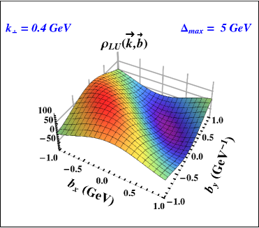
(a)    (b)

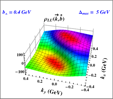
Figure 1: (Color online) 3D plots of the Wigner distributions $\rho_{LU}$. The plot (a) is in $b$ space with $k_{\perp}=0.4$ GeV. Plot (d) is in $k$ space with $b_{\perp}=0.4$ $GeV^{-1}$. We took $\Delta_{max}=5.0$ GeV. For all the plots we kept $m=0.33$ GeV, integrated out the $x$ variable and we took $\vec{k_{\perp}}=k\hat{j}$ and $\vec{b_{\perp}}=b\hat{j}$ [13].

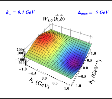
(a)    (b)

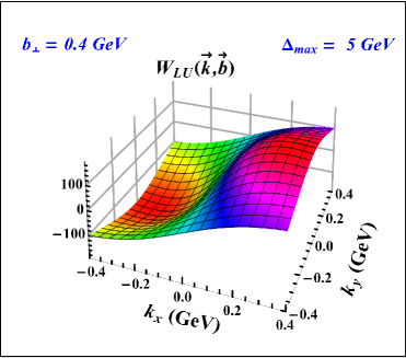
Figure 2: (Color online) 3D plots of the Wigner distributions $W^{LU}$. Plot (a) is in $b$ space with $k_{\perp}=0.4$ GeV. Plot (b) is in $k$ space with $b_{\perp}=0.4$ $\mathrm{GeV}^{-1}$. We have taken $\Delta_{max}=5.0$ GeV. For all the plots we kept $m=0.33$ GeV, integrated out the $x$ variable and we took $\vec{k_{\perp}}=k\hat{j}$ and $\vec{b_{\perp}}=b\hat{j}$ [14].

In Figs. 1 and 2, we have shown the 3D plots for the Wigner distributions $\rho_{LU}$ for the quarks and $W^{LU}$ for the gluons respectively in the impact parameter space ($b_{x}$-$b_{y}$) and in momentum space ($k_{x}$-$k_{y}$). The plots are taken from [13, 14]. Normally the upper limit of the Fourier transform should be infinite. But in our numerical calculation, we chose an upper limit of $\mid\Delta_{\perp}\mid$ called $\Delta_{max}$. The peak of the Wigner distribution increases in magnitude as $\Delta_{max}$ increases. For all the plots, we have taken mass of target state to be 0.33 GeV. Also we integrated over $x$ and divided by a normalization constant. $\rho_{LU}$ is the distortion of the Wigner distribution of unpolarized quarks due to the longitudinal polarization of the dressed quark. We observe a dipole structure in $b_{\perp}$ space, similar to that observed in other models. For the gluon distribution $W^{LU}$ we observe a similar behaviour.

3 Orbital angular momentum of quarks and gluons

The kinetic OAM for the quarks is given in terms of the GPDs [6] as :

$$L^{q}_{z}=\frac{1}{2}\int dx\{x[H^{q}(x,0,0)+E^{q}(x,0,0)]-\tilde{H^{q}}(x,0,0)\}.$$

The GPDs in the above equation are defined with the momentum transfer purely in the transverse direction. Using the GPDs in our model, we can calculate the kinetic quark OAM. The kinetic OAM is also related to the GTMDs [12] by the following relations:

$$H^{q}(x,0,t)=\int d^{2}k_{\perp}F_{11};$$ (14)

$$E^{q}(x,0,t)=\int d^{2}k_{\perp}\Big{[}-F_{11}+2\Big{(}\frac{k_{\perp}.\Delta_{\perp}}{\Delta_{\perp}^{2}}F_{12}+F_{13}\Big{)}\Big{]};$$ (15)

$$\tilde{H}^{q}(x,0,t)=\int d^{2}k_{\perp}G_{14}.$$ (16)

(a)    (b)

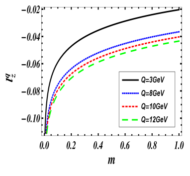
Figure 3: (Color online) Plots of quark OAM (a) kinetic and (b) canonical vs mass of the active quark (GeV). $Q$ is the upper limit of the transverse momentum in GeV [13]

The GTMD $F_{14}$ is related to the canonical OAM as shown in [11, 18, 19]:

$$l^{q}_{z}=-\int dxd^{2}k_{\perp}\frac{k_{\perp}^{2}}{m^{2}}F_{14}.$$ (17)

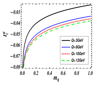
(a)    (b)

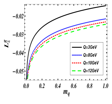
Figure 4: (Color online) Plots of gluon OAM (a) canonical and (b) kinetic vs mass of the active quark (GeV). $Q$ is the upper limit of the transverse momentum in GeV [14]

In order to calculate the gluon GTMDs we use the parametrization of in [20]. These can be related to the ones in [12]. Using this parametrization, one can relate the gluon GTMDs to the gluon kinetic and canonical OAM in the same way as for the quarks. In our model, the quark and gluon OAM can be calculated directly from the results for the Wigner distributions, as these are related to the GTMDs [13, 14]. Our results agree with [15] in the massless limit of the quark. We also agree with [21] and [22]. In our model calculation we find that the GTMDs $F_{14}$ and $G_{11}$ exist and non-zero. The result is independent of the choice of the gauge link at this order [22]. In Fig.3 we have shown the orbital angular momentum of quarks as a function of the mass as calculated in this model. Fig. 3(a) is for the kinetic OAM and 3(b) for canonical OAM. $Q$ is the upper limit in the transverse momentum integration, which is the large momentum scale involved in the process. Similar qualitative behavior of $L^{q}_{z}$ and $l^{q}_{z}$ are seen, however, the magnitude of the two OAM differs, this is due to the gluonic degrees of freedom in the model. In Figs. 4(a) and 4(b) we show the canonical and the kinetic gluon OAM respectively as a function of the quark mass. As in the quark case, we see that the magnitude of both the OAM decreases with increasing mass of target state.

The correlation between the quark spin and its OAM is given by [11, 23],

$$C^{q}_{z}=\int dxd^{2}k_{\perp}\frac{k_{\perp}^{2}}{m^{2}}G_{11}.$$ (18)

In this model $F_{14}$=$-G_{11}$, the above correlation is the same as the canonical OAM for the quarks. The gluon spin-orbit correlations can be related to the gluon GTMDs in a way similar to the above. Unlike for the quarks, canonical gluon OAM and spin-orbit correlations are different in this model. Another point to note is that the spin-orbit correlation for the quark in the dressed quark is negative. This is opposite to what is observed in chiral quark-soliton model and constituent quark model, namely here the quark spin is anti-aligned with its OAM.

4 Conclusion

We presented a recent calculation of the Wigner distributions for quarks and gluons. We took a simple composite spin-1/2 system which has a gluonic degree of freedom, namely a quark dressed with a gluon. We calculated the Wigner distributions both for unpolarized and longitudinally polarized target and quarks and gluons and investigated the correlations in transverse momentum and position space. We compared and contrasted the results for the quark distributions with calculations in light cone constituent quark model and light-cone chiral quark soliton model. For the gluon Wigner distributions, ours [14] are the first results. We also calculated the kinetic and canonical quark and gluon OAM and the spin-orbit correlations.

5 Acknowledgement

This work has been done in collaboration with Sreeraj Nair and Vikash K. Ojha [13, 14]. We thank the organizers of the QCD Evolution Workshop, 2015 at Jefferson lab for the invitation and hospitality.

References

- [1] X. Ji, Phys. Rev. Lett. 91, 062001 (2003).
- [2] A. Belitsky, X. Ji, F. Yuan; Phys.Rev. D 69, 074014 (2004).
- [3] J. Ashman et al., Nucl. Phys. B328, 1 (1989).
- [4] D. de Florian, R. sassot, M. Stratmann, W. Vogelsang, Phy. Rev. Lett. 113, No. 1, 012001 (2014); E. R. Nocera et al., NNPDF Collaboration, Nucl. Phys. B 887, 276 (2014).
- [5] R.L. Jaffe, A. Manohar, Nucl. Phys. B, B337 509 (1990)
- [6] X. Ji, Phys. Rev. Lett. 78,610 (1997).
- [7] M. Wakamatsu, Phys. Rev. D 81, 114010 (2010), Phys. Rev. D 83, 014012 (2011).
- [8] X.S. Chen, W.M. Sun, X.F. Lu, F. Wang, T. Goldman Phys.Rev.Lett. 100, 232002 (2008); Phys.Rev.Lett. 103, 062001 (2009)
- [9] M. Burkardt, Phys. Rev. D 88, 014014 (2013).
- [10] E. P. Wigner, Phys.Rev. 40, 749 (1932).
- [11] C. Lorce, B.Pasquini, Phys. Rev. D84, 014015 (2011).
- [12] S.Meissner, A.Metz,and M. Schlegel, JHEP 08 (2009) 056; S.Meissner, A.Metz, M. Schlegel and K. Goeke, JHEP 08 (2008) 038.
- [13] A. Mukherjee, S. Nair, V. K. Ojha Phys. Rev. D 90, 014024 (2014).
- [14] A. Mukherjee, S. Nair, V. K. Ojha Phys. Rev. D 91, 054018 (2015).
- [15] A. Harindranath and R. Kundu, Phys. Rev. D59, 116013 (1999).
- [16] X. Ji, X.Xiong and F.Yuan, Phys. Rev. D88, 014041 (2013).
- [17] W-M. Zhang and Harindranath, Phys. Rev. D48, 4881 (1993).
- [18] Y. Hatta, Phys. Lett. B 708, 186 (2012).
- [19] C. Lorce, B. Pasquini, X. Xiong, F. Yuan, Phys. Rev. D 85, 114006 (2012).
- [20] C. Lorce, B. Pasquini, JHEP 09 138 (2013)
- [21] Hikmat BC, M. Burkardt, Few Body Syst. 52, 389 (2012).
- [22] K. Kanazawa, C. Lorce, A. Metz, B. Pasquini, M. Schlegel, Phys. Rev. D90, 014028 (2014).
- [23] C. Lorce, Phys. Lett. B 735, 344 (2014).