A model for the slow dynamics of the supercooled liquid is formulated in terms of the standard equations of fluctuating nonlinear hydrodynamics (FNH) with the inclusion of an extra diffusive mode for the collective density fluctuations. If the compressible nature of the liquid is completely ignored, this diffusive mode sets the longest relaxation times in the supercooled state and smooths off a possible sharp ergodicity-nonergodicity (ENE) transition predicted in a mode coupling theory. The scenario changes when the complete dynamics is considered with the inclusion of $1/\rho$ nonlinearities in the FNH equations, reflecting the compressible nature of the liquid. The latter primarily determines the extent of slowing down in the supercooled liquid. The presence of slow diffusive modes in the supercooled liquid do not give rise to very long relaxation times unless the role of couplings between density and currents in the compressible liquid is negligible.

Ergodicity and slow diffusion in a supercooled liquid

I Introduction

The Mode coupling theory(MCT) has been developed as a microscopic theory to understand the slow dynamics of a supercooled liquid. The basic mechanism that increases the viscosity was first identified leth ; beng ; sjo-beng from kinetic theory of dense fluids. Subsequently equations of fluctuating nonlinear hydrodynamics (FNH) have been used to derive mybook ; kawasaki-jsp ; upen-pre ; prl2 the MCT. Generally, the defining expressions for these correlation functions are expressed in terms of space and time dependent transport coefficients. In the FNH formulation of the MCT, it is assumed that the crystallization process tu-frz ; sjo-psica does not interrupt and the transport coefficients are renormalized due to nonlinearities in the equations of motion for the slow modes and they are expressed in terms of hydrodynamic correlation functions. Nonlinear equations for the dynamics of the correlation functions are obtained from such definitions combined with the self consistent expressions for the transport coefficients. This gives rise to a feedback mechanism beng for slow relaxation of correlations spd-dufty in the supercooled liquid. As a consequence, the mode coupling theory (in its simplest form) predicts an ergodicty-nonergodicity (ENE) transition at a critical density $n_{c}$. The correlation function $\phi(q,t)$ of collective density fluctuations at wave vector $q$ and time separation $t$ is $f(q)\neq{0}$ at the transition.

In Ref. DM analysis of the fluctuating hydrodynamic equations for the compressible liquid showed how ergodicity is restored in the long time dynamics. The role of the $1/\rho$ yeomaj nonlinearities in the generalized equation for the momentum fluctuations in the compressible fluid played the key role in producing the ergodicity restoring mechanism. In a subsequent work Schimitz, Dufty, and De sdd has also considered a self-consistent mode coupling theory for supercooled liquids. The analysis presented by these authors demonstrates the absence of sharp transition to an ideal glassy phase DM in the model. In both the versions of mode coupling theories, respectively described in Ref.DM and Ref. sdd , the density correlation has an asymptotic behavior given by the form $[z+i\gamma(q,z)]^{-1}$, where the kernel $\gamma(q,z)$ can be expressed self-consistently in terms of hydrodynamic correlation functions giving rise to a diffusive decay. Subsequent to these works several other phenomenological models tu-kzip for the structural relaxation in a deeply supercooled glassy liquid sjo-tu were developed. Models taking into account orientational degrees of freedom tu-sd1 ; tu-sd2 has been proposed. From a qualitative level the breaking of the cage formation in the dense liquid is manifested through the couplings of current and density fluctuations. This process influences the dynamics and in particular mass transport in important ways. Orientational degrees of freedom has been included in description of the supercooled liquid to describe the process of cage formation and freezing at a local scale. In some of the works such phenomenological considerations were used to construct model biman-wolynes ; oppenheim1 ; oppenheim2 ; bpeak-pla by extending the existing self-consistent formulation of the MCT. From a general viewpoint the effects of activated events in some of these models are incorporated in the dynamics by using the concepts from the random first order transition theory. The dynamic structure factor is modified by localized activated hopping gtze-sjoren events termed in some works as instantons. Thus if we denote the density correlation function which acts like an order parameter in the MCT, as $\phi_{\mathrm{MCT}}(q,t)$, by including the so called hopping rmp it was modified as

$$\phi(q,t)\approx\phi_{\mathrm{MCT}}\phi_{\mathrm{hopp}}$$ (1)

It is argued that close to the glass transition temperature, $T_{g}$, since the configurational entropy $S_{c}$ is diminishing, the activated process slows down leading to an arrest of the structural relaxation. Beyond the mode coupling transition temperature, $T_{c}$, the density correlation is assumed to decay via the hopping channel. Thus the longitudinal viscosity, which is otherwise divergent in the idealized MCT, remains finite.

In the present work we propose a model in which instead of making a modification of standard MCT at the level of correlation function biman-wolynes ; das-schilling , with a diffusive mode, we modify the equations of FNH with the same, which forms the basis of the MCT. We include an extra diffusive processes in the collective density fluctuations in addition to the standard MCT. If the extra diffusive mode is ignored then our model reduces to the standard extended MCT model. The latter refers to the full mode coupling model in which all the important nonlinearities of the original equations of FNH are present. These nonlinearities include those which gives rise to an ergodicity-nonergodicity (ENE) transition at the simplest level, as well as the source of ergodicity restoring mechanism over longer time scales. The assumed diffusive mode is an additional mode in the system. Our analysis demonstrates the importance of the compressible nature of the liquid in determining the slow dynamics.

This basic model of extended MCT is obtained primarily from the conservation laws and the dynamics of the corresponding collective modes in the liquid. The Fluctuating Nonlinear Hydrodynamic modelsdd is formulated in terms of two fluctuating variables ${\bf g}$ and $\rho$ and without any $1/\rho$ nonlinearity present in the generalized equation for the momentum conservation. This involves simplifying the expression for the kinetic energy term $F_{K}$ of the driving free energy functional for the system which determines the equilibrium state of the liquid enz-tu . Making this change violates the Galilean invariance of the FNH equations. Since our focus here is primarily on the slow dynamics produced due to dominant density fluctuations we assume that this is not too important in the present analysis. The FNH equations studied in the present work are also based on a purely gaussian form of the driving free energy functional $F[\rho,g]$ like that of Ref. sdd and contains the same density and current coupling in the continuity equation as in Ref. sdd . In this model of extended MCT, the ENE transition is smeared off due to this density and current coupling appearing in the continuity equation. On ignoring this nonlinearity in the continuity equation, we get the basic MCT model which predicts an ENE transition at a critical density. As noted above additionally, we include here a diffusive mode as an extra slow process in the dense supercooled state of the liquid. With this the continuity equation is now modified and the corresponding current have contributions from the diffusive mode as well as the random noise. The form of a balance equation for the density variable is maintained. The dissipative term in the equation of motion for the collective density field $\rho({\bf x},t)$ is linear. If this diffusive mode and the related noise is ignored then our model reduces to the FNH model of Ref. sdd . The goal of the present analysis is to study how the simultaneous presence of the diffusive mode and $1/\rho$ nonlinearities affects the dynamics and determine their relative importance in producing the slow dynamics.

The paper is organized as follows. In the next section we discuss the construction of the basic equations of FNH using standard formalisms Oldbook but adopting a purely gaussian free energy functional. This is followed in section III by discussion of linearized dynamics and the noise averaged correlation functions. In the next section VI we construct the renormalized theory taking into account one loop expressions for the self energies renormalizing the transport coefficients. Section V discusses the numerical solution of the MCT equations and is followed by discussion section.

II Model studied

The basic equations of the model for the dynamics of a fluid is obtained using the standard techniquesOldbook ; tur1-hyd ; tur2-hyd of fluctuating nonlinear hydrodynamics (FNH). The equation of motion for the coarse grained density $\rho({\bf x},t)$ is a continuity equation with the momentum density ${\bf g}({\bf x},t)$ as the current which itself is a conserved property. The current ${\bf g}({\bf x},t)$ satisfies the momentum conservation equation. The latter constitutes the generalized Navier-Stokes equation. We include in the present work an additional dissipative term and a noise in the continuity equation. The two are related by a standard fluctuation-dissipation relation.

II.1 Generalized Langevin Equations

We begin with the coarse grained mass density ${\rho}({\bf x},t)$  and the momentum density  ${\bf g}_{i}({\bf x},t)$ constitute the set of slow variables for the liquid. In the standard formulation of Fluctuating nonlinear hydrodynamics these variables satisfy the Langevin dynamics with following the generalized formma-mazenko for the equation of motion,

$$\frac{\partial\psi_{i}}{\partial t}=V_{i}[\psi_{i}]-L^{0}_{ij}\frac{\delta{F}}{\delta\psi_{j}}+\theta_{i}~{}~{}.$$ (2)

In the above equation and throughout this paper we follow the notation that repeated indices are summed over. $V_{i}[\psi_{i}]$ is the ”streaming velocity” term representing the reversible part of the dynamics, and is obtained as

$$V_{i}({\bf x}) = Q_{ij}\frac{\delta{F}}{\delta{\psi_{j}}}$$

where $Q_{ij}{\equiv}\{\psi_{i},\psi_{j}\}$ is Poisson bracket between slow variables $\psi_{i}$ and $\psi_{j}$. The driving free energy is a functional of the slow modes in FNH description and is written as a sum of two parts here,

$$F[\psi]=F_{K}[\psi]+F_{U}[\psi]~{}~{}.$$ (3)

The kinetic partlanger and the potential part of free energy functional with the variables $\{\rho,{\bf g}\}$ are respectively given by

$$F_{K}[g] = \int d{\bf x}~{}~{}\left[\frac{g^{2}({\bf x})}{2\rho_{0}}\right]$$ (4)

$$F_{U}[\rho] = \frac{1}{2}\int d{\bf x}~{}\int d{\bf x}^{\prime}~{}\delta\rho({\bf x})\chi_{\rho\rho}^{-1}({\bf x}-{\bf x}^{\prime})\delta\rho({\bf x}^{\prime})~{}~{}.$$ (5)

$\chi^{-1}_{\rho\rho}$ denotes the inverse of the static (equal time) correlation function of density fluctuations and is related to the static structure factorhansen of the liquid. The above choice of the free energy functional is of a purely gaussian in both fields $\rho$ and ${\bf g}$. The formulation of the equations of fluctuating nonlinear hydrodynamics (FNH) is standard DM . We provide here a few details specific for the present model. With the choice (3)-(5) the streaming energy term for the FNH equations ( signifying reversible dynamics) for density $\rho$ and momentum density ${\bf g}$ are different from the standard results DM . Nonlinearities appear in the streaming term $V_{\rho}$ for the density equation, while gallelian invariance term in the corresponding $V_{g_{i}}$ for momentum density $g_{i}$ is different. The streaming velocities of  $\rho$ and ${\bf g}$  fields are obtained as:

$$V_{\rho}(\bf x) = -\nabla.\left[\frac{{\bf g}({\bf x})\rho(\bf x)}{\rho_{0}}\right]$$ (6)

$$V^{i}_{g}(\bf x) = -\rho({\bf x})\nabla_{\bf x}^{i}\frac{\delta{F_{U}}}{\delta\rho({\bf x})}-\nabla_{\bf x}^{j}\left[\frac{g_{i}({\bf x})g_{j}({\bf x})}{\rho_{0}}\right]-\nabla_{\bf x}^{i}\left(\frac{g^{2}({\bf x})}{2\rho_{0}}\right)$$

The standard form for the free energyDM is one in which the $1/\rho_{0}$ in the expression for $F_{K}$ is replaced by a $1/\rho$ term. The corresponding $F_{K}$ gives a continuity equation which is essential for the microscopic momentum conservation with the current density ${\bf g}$. This choice for $F_{K}$ also produces the proper nonlinear term in the momentum equation needed for maintaining the Galilean invariance in the FNH equations. The advantage of using the present form is that the free energy $F[g,\rho]$ remain gaussian. As a result the dissipative terms in the dynamical equations ( $\sim\delta{F}/\delta{\psi}$ ) are linear in the hydrodynamic variables.

The time reversal properties of dissipative terms are given by that of the corresponding transport coefficients,

$$L^{0}_{ij}(-t)=\epsilon_{i}\epsilon_{j}L^{0}_{ij}(t)~{}~{}.$$ (8)

Here $\psi_{i}(-t)=\epsilon_{i}\psi(t)$. Thus the dissipative terms like $L^{0}_{g\rho}$ are zero. We have $L^{0}_{\rho\rho}(-t)=L^{0}_{\rho\rho}(t)$ is nonzero. Similarly $L^{0}_{g_{i}g_{j}}$ is also survives the time reversal symmetry. In the present model dissipative terms are present in both the density and momentum equations. As a result, both equations have respective random noise components as well. These noises in the $\rho$ and ${\bf g}$ equations are respectively denoted as  $f$  and  $\theta$. The random part of the density equation is expressed in terms of a force vector ${\bf f}_{R}$ such that ${f}=\nabla.{\bf f}_{R}$. The corresponding noise correlation functions are given by the standard fluctuation dissipation relations.

$$\langle f_{R}^{i}({\bf x},t)~{}f_{R}^{j}({\bf x}^{\prime},t^{\prime})\rangle = 2k_{B}T~{}\delta_{ij}~{}L_{\rho}\delta({\bf x}-{\bf x}^{\prime})~{}\delta(t-t^{\prime})$$

$$\langle\theta_{i}({\bf x},t)~{}\theta_{j}({\bf x}^{\prime},t^{\prime})\rangle = 2k_{B}T~{}L^{0}_{ij}\delta({\bf x}-{\bf x}^{\prime})~{}\delta(t-t^{\prime})$$

where we have taken the dissipative coefficient in the density equation as in the equation as $L^{0}_{\rho\rho}={L_{\rho}}\nabla^{2}$.

Using the Poisson brackets between the slow variablesvolvick described in the appendix A, the generalized Langevin equation of motion for $\rho$  having both dissipative and random parts is obtained as

$$\frac{\partial\rho}{\partial t}+\nabla.\left({\bf g}({\bf x})\frac{\rho}{\rho_{0}}\right)-\gamma_{0}\nabla^{2}{\rho({\bf x})}=f~{}~{},$$ (9)

where $\gamma_{0}={L_{\rho}}\chi^{-1}_{\rho\rho}$. The above equation is written in the form of a continuity equation as

$$\frac{\partial\rho}{\partial t}+\nabla.\tilde{\bf g}=0~{}~{},$$ (10)

with the generalized current $\tilde{\bf g}(\bf x,t)$ obtained as

$$\tilde{\bf g}={\bf g}+\frac{\delta\rho}{\rho_{0}}{\bf g}-\gamma_{0}{\bf\nabla}\rho-{\bf f}_{R}~{}~{}.$$ (11)

which is different from ${\bf g}(\bf x,t)$ appearing in the first term on the right hand side. The field ${\bf g}$ is such that its dynamics is described by the generalized Langevin equation (2), and the reversible part of its dynamics being given in terms Poisson brackets for the microscopic field ${\bf g}$. The generalized Langevin equation of motion for ${\bf g}$  field is given as

$$\frac{\partial g_{i}}{\partial t}+\nabla_{j}\left[\frac{g_{i}g_{j}}{\rho_{0}}\right]+\nabla_{i}\left[\frac{g_{i}^{2}}{2\rho_{0}}\right]+\rho\nabla_{i}\frac{\delta F_{U}}{\delta\rho}+{\tilde{L}}^{0}_{ij}{g_{j}}=\theta_{i}~{}~{}.$$ (12)

In a normal fluid the diffusive mode is absent and the two quantities ${\bf g}$ and $\tilde{\bf g}$ are the same. We have defined the matrix of kinematic viscosity coefficients in terms of $\tilde{L}^{0}_{ij}=L^{0}_{ij}/{\rho_{0}}$ and the nonzero bare transport matrix elements are obtained as

$$L^{0}_{ij}=-\eta_{0}[\frac{1}{3}\nabla_{i}\nabla_{j}+\delta_{ij}\nabla^{2}]-\zeta_{0}\nabla_{i}\nabla_{j}~{}~{}.$$ (13)

$\zeta_{0}$ and $\eta_{0}$ respectively denotes the bulk and shear viscosities of the liquid. Equation (12) does not imply microscopic conservation for the total momentum current $\tilde{\bf g}$ appearing in the continuity equation.

As a result of using the purely gaussian free energy functional there are several changes in the equations of motion:

(a) The convective nonlinearity of the standard form $\nabla_{j}[g_{i}g_{j}/\rho]$ which is essential for Galilean invariance is now absent from the equation for the momentum density g;

(b) The equations of motion must have the Poission bracket between slow variables unchanged and the detailed balance condition $Q_{ij}=-Q_{ji}$ is not compromised.

As a result the continuity equation now contain extra density-momentum nonlinearities. These additional bi-linearities eliminate the structural arrest predicted by mode coupling theories with only density-density nonlinearities in the Pressure term das-PRL84 . Interestingly, the form of the cutoff function in this model, responsible for the removal of the sharp transition, is identical at the one loop order to the same quantity in the analysis presented in Ref. das-PRE96 . This holds even when the diffusive mode in collective density fluctuations is ignored. In the next section we consider the implications of the full nonlinear model with both the diffusive mode and density current nonlinearities being present.

The issue of the microscopic momentum conservation in the present model is special. The FNH equations considered here are plausible generalizations of the long time, long length scale hydrodynamics. The continuity equation is maintained in the present model at the microscopic level, i.e., with the microscopic definition of density $\hat{\rho}$ in terms of delta functions we obtain a continuity equation with a corresponding microscopic momentum density $\hat{\bf g}$. On averaging the microscopic continuity equation we obtain a similar equation (10) involving the coarse grained densities. The coarse grained current is $<\hat{\bf g}({\bf x},t)>{\equiv}\tilde{\bf g}({\bf x},t)$, defined in the Eqn. (11). Note that the current ${\bf g}({\bf x},t)$ which satisfies the balance Eqn. (12) is different from the coarse grained current $\tilde{\bf g}$. With this interpretation, the flux in the continuity equation for density $\rho({\bf x},t)$, i.e., $\tilde{\bf g}$ does not follow a balance equation and hence the momentum conservation is not preserved. On the other hand, if we take ${\bf g}$ as the coarse grained momentum density current, the continuity equation and Gallelian invariance are both violated. In systems with microscopic Brownian dynamics for which the mode coupling models, such as the present one, are often applied, momentum conservation is not satisfied though not implied in the strict microscopic sense. For the frozen amorphous state, the momentum fluctuations decay out much faster compared to the density fluctuations. Thus for the decay of density fluctuations approximations without strict momentum conservation is assumed. Works of Kawasakikawa-miya ; munakata obtaining the Dean-Kawasaki equationsdean using the so called adiabatic or over-damping approximation of the momentum equation are similar in this respect. Even in systems with Newtonian dynamics this approximation is applied for studying glassy behavior using density as the only relevant collective variable.

II.2 Correlation and Response functions

We use the standard field theoretic method of Martin-Siggia-Rose (MSR)msr ; jensen ; wagner ; hca1 ; hca2 ; hca3 in order to obtain the perturbative corrections due to the various nonlinearities. The full matrix ${\bf G}$ of correlation between the various fields, respectively at two different space time points (denoted as 1 and 2) includes the correlation functions and the response functions. These are respectively defined as

$$G_{\alpha\beta}(12) = \langle\psi_{\beta}(2)\psi_{\alpha}(1)\rangle$$ (14)

$$G_{\alpha\hat{\beta}}(12) = \langle\hat{\psi}_{\beta}(2)\psi_{\alpha}(1)\rangle$$ (15)

The Greek letter subscripts refer to the set of physical fields $\{\psi\}\equiv\{\rho,{\bf g}\}$ and their respective hatted counterparts $\hat{\psi}\equiv\{\hat{\rho},\hat{\bf g}\}$. The averages are functional integrals over all the fields weighted by $\exp[-{\cal A}]$ where the action functional ${\cal A}$ is obtainedDM as

$${\cal A}[\psi,\hat{\psi}]\equiv{\cal A}_{0}[\psi,\hat{\psi}]+{\cal A}_{I}[\psi,\hat{\psi}]$$ (16)

using the generalized Langevin equations. ${\cal A}_{0}$ and ${\cal A}_{I}$ denote the gaussian (quadratic in the fields) and nongaussian parts originating respectively from the linear and nonlinear parts of the equations of motion for $\{\rho,{\bf g}\}$. Using the equations of motion for the $\rho$ and ${\bf g}$ fields we obtain the MSR action functional involving the conjugate fields $\{\hat{\rho},\hat{\bf g}\}$ of the MSR approachmybook in the following form.

$${\cal A}[\psi,\hat{\psi}] = \int d1\Bigg{[}\beta^{-1}\Big{\{}\hat{\rho}(1)\gamma_{0}\chi_{\rho\rho}\nabla^{2}\hat{\rho}(1)+\hat{g}_{i}(1)L^{0}_{ij}(1)\hat{g}_{j}(1)\Big{\}}$$

$$+ i\hat{\rho}(1)\Big{\{}\Big{(}\frac{\partial\rho(1)}{\partial t}+\nabla.{\bf g}(1)-\gamma_{0}\nabla^{2}\rho(1)\Big{)}+\nabla.\Big{(}{\bf g}(1)\frac{\delta\rho(1)}{\rho_{0}}\Big{)}\Big{\}}$$

$$+i\hat{g}_{i}(1)\Big{\{}\frac{\partial g_{i}(1)}{\partial t} + \rho(1)\nabla_{i}\chi^{-1}_{\rho\rho}{\delta\rho(1)}+{\tilde{L}}^{0}_{ij}{g}_{j}(1)+\nabla_{j}\left[\frac{g_{i}(1)g_{j}(1)}{\rho_{0}}+\delta_{ij}\frac{g_{j}^{2}(1)}{2\rho_{0}}\right]\Big{\}}\Bigg{]}$$ (18)

$$\equiv {\cal A}_{0}[\psi,\hat{\psi}]+{\cal A}_{I}[\psi,\hat{\psi}]$$

In writing the above form of the action we have used the equation of motion (12) corresponding to the Gaussian form of the driving free energy functional (5). The inverse of zeroth order matrix  $G_{\alpha\beta}^{0}$  corresponding to the gaussian part ${\cal A}_{0}$ of the above action functional (II.2) is given in table 1.

II.3 Fluctuation-Dissipation Relations

The transformations which keep the MSR action invariant are written in terms of the field $\psi_{i}$ as

$$\psi_{i}({\bf x},-t) \rightarrow \epsilon_{i}\psi_{i}({\bf x},t)$$ (19)

$$\hat{\psi}_{i}({\bf x},-t) \rightarrow -\epsilon_{i}\left[\hat{\psi}_{i}({\bf x},t)-i\beta\frac{\delta F}{\delta\psi_{i}({\bf x},t)}\right],~{}~{}$$ (20)

For example, we use the above transformation to obtain the FDT’s. Using the transformation for the $\rho$ field

$$\rho({\bf x},-t) \rightarrow \rho({\bf x},t)$$ (21)

$$\hat{\rho}({\bf x},-t) \rightarrow -\left[\hat{\rho}({\bf x},t)-i\beta\frac{\delta F}{\delta\rho({\bf x},t)}\right]~{}~{}.$$ (22)

Using these time reversal invariance propertiesABL ; DM of the action ${\cal A}$, a set of fluctuation-dissipation relations (FDR) linking the correlation and response functions is obtained.

$$G_{g_{j}\beta}(q,\omega) = -2\beta^{-1}\rho_{0}{\rm Im}[G_{\hat{g}_{j}\beta}(q,\omega)]$$ (23)

$$G_{\rho\beta}(q,\omega) = -2\beta^{-1}\chi_{\rho\rho}{\rm Im}[G_{\hat{\rho}\beta}(q,\omega)]~{}~{},$$ (24)

where $\beta$ is an un-hatted variable. This model have a complete set of FDR linearly relating correlation and response functions. This is a consequence of having gaussian free energy functional ABL ; DM09 ; jsp2-ene . To summarize, using the time translational invariance properties of the action (II.2), the fluctuation dissipation relation between correlation and response functions involving the field $\hat{\psi}$ and $\varphi$ are obtained in the form :

$$G_{\zeta_{\psi}{\varphi}}({\bf q},\omega)=-2\beta^{-1}{\rm Im}G_{\hat{\psi}\varphi}({\bf q},\omega),$$ (25)

where $\zeta_{\psi}$ is expressed as a functional derivative of the free energy functional with the field $\psi$:

$$\zeta_{\psi}({\bf x})=\frac{\delta F}{\delta\psi({\bf x})}~{}~{}.$$ (26)

In the present case since $F$ is quadratic in the fields $\{\rho,{\bf g}\}$, the function $\zeta$ is linear in the fields. Hence the resulting FDT’s are therefore linearmazenko-book .

II.4 Renormalized Dynamics

In this section we discuss how the nonlinearities in the FNH equations renormalize the dynamics using standard field theoretic techniques. The role of the nonlinearities in the dynamics is expressed in terms of the self energy matrix $\Sigma$ defined through the Dyson equation

$${\bf G}^{-1}(1,2)={\bf G}^{-1}_{0}(1,2)-\Sigma(1,2),~{}~{}$$ (27)

where $G_{0}^{-1}$ and $G^{-1}$ respectively denote the inverse of the correlation matrices obtained with gaussian action ${\cal A}_{0}$ and full action ${\cal A}$. The key quantity which determined the renormalization of the correlation function matrix from ${\bf G}_{0}$ to ${\bf G}$, is the self energy matrix $\Sigma$.

In the Appendix A we give a brief description of the structure of the Green’s function matrix in this problem. We demonstrate that by inverting the matrix ${\bf G}^{-1}$, the correlation functions of collective modes are obtained in a form which is real by construction and involves the response type correlations between hatted and un-hatted fields. The renormalized correlation and response functions are now expressed in terms of renormalized transport coefficients as shown in Eqn. (A). The renormalization of the transport coefficients in the model due to the nonlinearities in the equations of motion for the collective modes is a key ingredient in the present analysis. We briefly outline the details of obtaining the expressions for correlation functions (44) and response functions (46) using the MSR formalism in the Appendix A. The renormalizability is demonstrated here in the hydrodynamic limit. To understand this we need to analyze the nature of the renormalized theory in the present case. We note the following points specific to the present model and essential for further analysis.

• The FDR relations between the correlation ($G_{\psi\psi}$) and response functions ($G_{\psi\hat{\psi}}$) of the MSR theory presented here are linear.

• The Dyson equation (27) links inverse of ${\bf G}$ and ${\bf G}_{0}$. Effects of nonlinearities are accounted for through the self energy matrix $\Sigma$. The elements of the zeroth order Green’s functions ${\bf G}^{-1}_{0}$ involve only the bare transport coefficients. The corresponding full ${\bf G}$ for the nonlinear dynamics involve the respective renormalized transport coefficients.

• The matrices ${\bf G}_{0}^{-1}$ and ${\bf G}^{-1}$ both have correlation ($\psi\psi$) and response ($\psi\hat{\psi}$) elements which are expressed in terms of transport coefficients. For ${\bf G}^{-1}_{0}$ it is only bare transport quantities. For ${\bf G}^{-1}$, the corresponding self energy elements appearing respectively in its correlation and response elements must be linked to each other ensure that the renormalized transport coefficients are unique. However the full $G^{-1}$ matrix is not simply obtained from the $G_{0}^{-1}$ with bare quantities being replaced by renormalized transport coefficients. Some of the elements of $\Sigma$ are nonzero though the corresponding element for ${\bf G}_{0}^{-1}$ matrix are zero. Thus for the full theory, a linear FDR between the elements of ${\bf G}$ does not translate in to a similar relation between the corresponding elements of $\Sigma$. Similar relations we have established here hold only in the hydrodynamic limit.

III Dynamics of Correlation functions

Using the linear FDR relactions (23)-(24) we obtain that the Laplace transformation of three correlation functions are

$${\cal D}\psi_{\rho\rho}(q,z) = {z+iq^{2}L(q,z)}$$ (28)

$${\cal D}\psi_{gg}(q,z) = {z+iq^{2}\gamma(q,z)}$$ (29)

$${\cal D}\psi_{\rho g}(q,z) = -iqc$$ (30)

where the denominator ${\cal D}$ has been defined in Eqn. (47) in the Appendix A. From the above relations we obtain the density correlation function as,

$$\frac{1-z\psi_{\rho\rho}}{\psi_{\rho\rho}}+\frac{q^{2}c^{2}}{z+iq^{2}L(q,z)}=iq^{2}\gamma(q,z)~{}~{}.$$ (31)

The term $\gamma$ appearing on the right hand side of the above equation is the sum of the contributions from the self energy $\gamma_{\hat{\rho}\rho}$ and the bare diffusion process $\gamma_{0}$ introduced here. The self energy contribution arises from the bilinear couplings of density and momentum in the continuity equation (10). In absence of this coupling, the self energy with $\gamma_{\hat{\rho}\rho}$ is zero. If both the bare diffusion and density-current couplings are absent, the continuity equation has the flux ${\bf g}$ and we obtain the standard form of the density correlation function.

$$\psi_{\rho\rho}(q,z) = \frac{z+iq^{2}L(q,z)}{z[z+iq^{2}L(q,z)]-q^{2}c^{2}}$$

$$\psi_{\rho{g}}(q,z) = \frac{-iqc}{z+iq^{2}L(q,z)}\psi_{\rho\rho}(q,z)$$ (32)

By doing an inverse Laplace transform of the Eqns. (28)-(30), a set of integro-differential equations for the time evolution of the correlation functions $\{\psi_{\rho\rho}(q,t),\psi_{\rho{g}}(q,t),\psi_{gg}(q,t)\}$ are obtained. A fully wave vector dependent solution of the problem is very involved. We focus here on the basic features of the mode coupling dynamics, suppressing all wave vector dependence. In the schematic form of the model, wave vector dependence of the correlation functions are dropped obtaining the following set of coupled equations for the time dependent correlation functions:

$$\ddot{\psi}_{\rho\rho}(t)+\kappa^{2}\Bigg{[}\psi_{\rho\rho}(t)+\gamma(t)+\int_{0}^{t}d\tau\left[L(t-\tau)+\gamma(t-\tau)\right]\dot{\psi}_{\rho\rho}(\tau)$$ (34)

$$+ \kappa^{2}\int_{0}^{t}d\tau\gamma(t-\tau)\int_{0}^{\tau}{d\tau^{\prime}}\Big{[}L(\tau-\tau^{\prime})\psi_{\rho\rho}(\tau^{\prime})\Big{]}\Bigg{]}=0~{}~{}$$

$$\dot{\psi}_{gg}(t)=\dot{\psi}_{\rho\rho}(t)-\kappa^{2}\int_{0}^{t}d\tau\left[L(t-\tau){\psi}_{gg}(\tau)-\gamma(t-\tau){\psi}_{\rho\rho}(\tau)\right]$$

$$\dot{\psi}_{\rho{g}}(t)=-\kappa~{}\psi_{\rho\rho}(t)-\kappa^{2}\int_{0}^{t}d\tau L(t-\tau){\psi}_{\rho{g}}(\tau)~{}~{}.$$

In the above equation we have denoted the wave vector $q$ scaled with an upper cutoff $\Lambda$ as $\kappa=q/\Lambda$. Time has been rescaled in units of $\tilde{L}_{0}/c^{2}$ involving the bare (kinematic) longitudinal viscosity $\tilde{L}_{0}=L_{0}/\rho_{0}$. Hence frequency is scaled in units of $c^{2}/\tilde{L}_{0}$. We also take the dimensionless quantity $(\Lambda\tilde{L}_{0}/c)=1$. Assuming wave vector independent structure function $\chi$ (say), the mode coupling integrals are expressed in terms of the dimensionless coupling constant $\lambda=\Lambda^{3}/(6\pi^{2}{c^{2}}\beta\rho_{0})$. In the schematic model all wave vector dependence of the theory is incorporated through the parameter $\lambda$. To properly account for the structural effect, this dependence should be replaced by that of the static (equal time) correlation functions. The latter depend on the thermodynamic parameters for the liquid state. The renormalized memory functions are obtained as a sum of the bare and mode coupling parts,

$$L(t) = \delta(t)+L^{mc}(t)$$ (35)

$$\gamma(t) = \Delta_{0}\delta(t)+\gamma^{mc}(t)~{}~{},$$ (36)

where the constant $\Delta_{0}$ is proportional to the diffusion constant $\gamma_{0}$ corresponding to the slow mode introduced in the continuity equation. In terms of the bare longitudinal viscosity $\tilde{L}_{0}$ of the liquid we define

$$\Delta_{0}=\frac{\gamma_{0}}{\tilde{L}_{0}}$$ (37)

$L^{mc}(t)$ and $\gamma^{mc}(t)$ are both nonlinear functional of $\psi_{\rho\rho}(t)$, ${\psi}_{\rho{g}}(t)$, and ${\psi}_{gg}(t)$. At one loop level we obtain these quantities from a diagrammatic calculation of the memory functions, dropping all wave vector dependence. The corresponding one loop diagrams for the self energies $\gamma_{\hat{g}\hat{g}}$ and $\gamma_{\hat{\rho}\hat{\rho}}$ respectively representing the renormalization of the viscosity and the ergodicity restoring mechanisms, are shown in Fig. 1-2. The memory functions $L^{mc}$ and $\gamma^{mc}$ are respectively obtained as

$$L^{mc}(t) = \lambda\psi_{\rho\rho}^{2}(t)$$ (38)

$$\gamma^{mc}(t) = \frac{\lambda}{3}~{}\Big{[}\psi_{\rho\rho}(t)\psi_{gg}(t)+\psi_{\rho{g}}(t)\psi_{g\rho}(t)\Big{]}~{}~{}.$$ (39)

The definitions (38)-(39) form a closed set of nonlinear equations (34)-(34) for the correlation function. If we set the extra diffusive mode of $\gamma_{0}$ to be zero then this model is same as what was proposed in Ref. sdd . We refer this as SDD model and the corresponding $\gamma^{mc}$ as $\gamma_{SDD}$.

$$\gamma(t)=\gamma^{mc}(t)=\gamma_{SDD}~{}~{}.$$ (40)

In the following we also consider the case in which we obtain $\gamma^{mc}$ to leading order in $\lambda$ or the density-momentum nonlinearity of the continuity equation. In this approach, we replace the correlation function $\psi_{\rho{g}}$ and $\psi_{gg}$ in terms of derivatives of density correlation function $\psi_{\rho\rho}$ at lowest order in the perturbation theory ( in terms of the ${\bf g}\delta\rho$ coupling). This will be the one loop approximation for the function $\gamma^{mc}(t)$. In presence of the intrinsic diffusive mode $\Delta_{0}$ the $\gamma$ denoted as $\gamma_{DM}$.

$$\gamma^{mc}(t){\equiv}=\gamma_{DM}={2\lambda}\Big{[}\dot{\psi}_{\rho\rho}^{2}(t)-\frac{2\Delta_{0}}{3}\dot{\psi}_{\rho\rho}(t)\psi(t)-\frac{\Delta^{2}_{0}}{5}\psi_{\rho\rho}^{2}(t)\Big{]}{\equiv}\gamma_{DM}.$$ (41)

$\dot{\psi}_{\rho\rho}(t)$ above refers to derivative with respect to time and so on. The decay of the correlation functions with both $\gamma_{DM}$ and $\gamma_{SDD}$ will be presented in the following section.

IV Numerical Results

In order to analyze the implications on the ENE transition we focus on the above integro differential equation (34)-(34). Numerical solution of the above set of schematic equations for the correlation function provides insight in to the nature of the dynamics under various circumstances. In the extended mode coupling model considered here there are clearly two mechanisms competing with each other in eliminating the sharp ENE transition. These are

A. The bilinear couplings of density and current ( ${\bf g}\delta\rho$) in the compressible liquid present in the continuity equation similar to Ref. sdd . This is represented by the ${\bf\nabla}\cdot[({\bf g}/\rho)\delta\rho]$ term in the continuity equation (10).

B. The presence of the slow mode with diffusion constant $\gamma_{0}$ for density fluctuations.

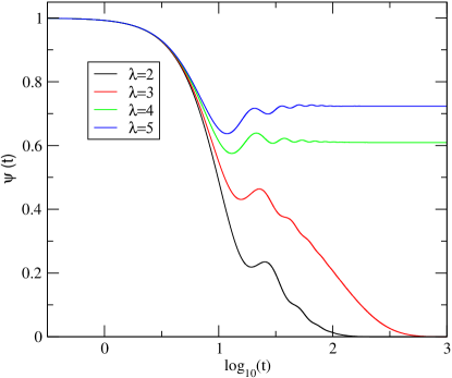
Figure 3: The density correlation function $\psi(t)$ Vs. log(t) for different values of the thermodynamic parameter $\lambda$ (see text) with a sharp ENE transition at $\lambda=4$. Here all ergodicity restoring process have been ignored

If we remove both processes A and B, by ignoring the density momentum coupling int the continuity equation and setting $\gamma_{0}=0$, then the model is the simple MCT model leth with an ideal transition. In Fig. 3 the results for the density correlation function $\psi_{\rho\rho}(t)$ for this simple case is shown for different values of the parameter $\lambda$. The liquid undergoes an ideal ENE transition at the point $\lambda=\lambda_{c}=4$ in the model. With increasing $\lambda$ the density correlation function relaxes slower and eventually freezes at a nonzero value beyond $\lambda=4$.

IV.1 Dynamics of SDD Model

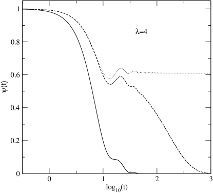
Figure 4: The density correlation function $\psi(t)$ Vs. log(t) for the thermodynamic parameter $\lambda=4$ and $\gamma_{0}=0$. With the cutoff function $\gamma^{mc}$(see text) set to a) zero(dotted), b) $\gamma_{SDD}$(solid), and c) $\gamma_{DM}$ (dashed).

To consider the extended model without the ENE transition we first take the case in which process A is included while the diffusive process of B is absent. With this choice ($\Delta_{0}=0$) the present model becomes identical to what was earlier considered in Ref. sdd . It is well knownsdd ; das-PRE96 that the inclusion of bilinear couplings in the density and momentum in the continuity equation produce the cut off mechanism responsible for the restoration of the ergodicity in this model. The corresponding cut off function $\gamma^{mc}(t)$ is now obtained either in the form $\gamma_{SDD}$ or $\gamma_{DM}$ stated above. The mode coupling effects are considered in the expressions (40) and (41) at the one loop level. In both cases due to contributions coming from the density and current couplings, ergodicity is restored in the final decay of the correlation function. In terms of the density dependent parameter $\lambda$ we obtain the decay of the correlation functions. In Fig 4-6, we show the density correlations respectively for the parameter values $\lambda=4,$ $6$, and $8$. In each of these figures, we display the correlation functions obtained corresponding to different choices for the cut off function $\gamma^{mc}$ : set equal to a) zero (dotted), b) $\gamma_{SDD}$ (solid), and c) $\gamma_{DM}$ (dashed).

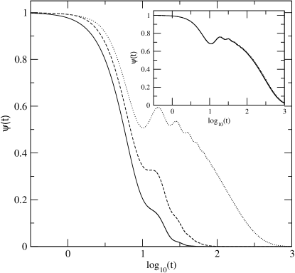
Figure 7: The density correlation function $\psi(t)$ Vs. log(t) for the thermodynamic parameter $\lambda=4$ and $\Delta_{0}=0$. With the cutoff function $\gamma_{SDD}$ set to start from a time $t_{0}=0$(solid), $1$(dashed), and $2$(dotted). Inset shows the same results with the corresponding cutoff function as $\gamma_{DM}$

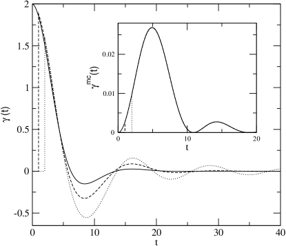
Figure 8: The cutoff function $\gamma^{mc}(t)$ Vs. $t$ for the results shown in Fig 7 in the main and inset respectively.

Another approach to understanding slow dynamics involves assuming that the ergodicity restoring mechanisms are effective beyond an initial time. The idea is to introduce a lower cutoff time $t_{0}$ from when the cutoff process is assumed to become effective henk-t0 ; jcp-t0 . The role of $t_{0}$ on the dynamics of the density correlation function is explored in Fig. 7. The main figure shows the results for $\psi_{\rho\rho}(t)$ vs. $t$ with $\gamma^{mc}{\equiv}\gamma_{SDD}$ for three different choices of $t_{0}=0,1,$ and $2$. With $\gamma^{mc}$ being determined from $\gamma_{DM}$ the effect of $t_{0}$ is less on the long time dynamics of $\psi_{\rho\rho}(t)$ as shown in the Inset of Fig. 7. The corresponding cutoff functions $\gamma_{SDD}(t)$ and $\gamma_{DM}(t)$ are displayed in Fig. 8.

IV.2 Inclusion of a diffusive mode

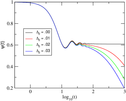
Figure 9: The density correlation function $\psi(t)$ Vs. log(t) for different diffusion coefficients $\Delta_{0}$. The density-current coupling of Ref. sdd is absent here and $\lambda=4$.

Next, we consider the case in which the process A is excluded but the diffusive mode of B is present. This means that the bilinear density and momentum coupling in the continuity equation is ignored but the extra diffusive mode is included in the theory taking $\gamma_{0}$ nonzero. The result of this model is shown in Fig. 9. We plot density correlation function $\psi_{\rho\rho}$ vs. $t$ for different choices of the relative bare diffusion coefficients $\Delta_{0}$ (defined in Eqn. (37). With increase of $\Delta_{0}$, the density correlation function decays faster. The value of $\lambda$ used in this figure is kept constant at $\lambda_{c}=4$.

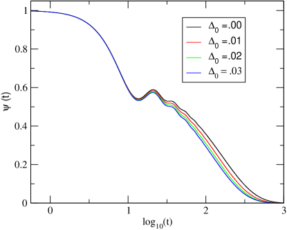
Figure 10: The density correlation function $\psi(t)$ Vs. log(t) for different diffusion coefficients $\Delta_{0}$ together with the density-current coupling of Ref sdd being present. $\lambda=4$.

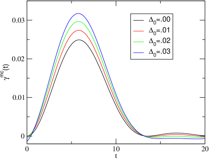
Figure 11: The cutoff function $\gamma^{mc}(t)$ Vs. $t$ for the results shown in Fig 10.

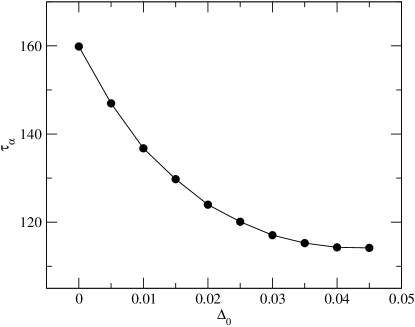
Figure 12: The relaxation time $\tau_{\alpha}$ (see text) for the density correlation function shown in Fig 10 vs. diffusion constant $\Delta_{0}$.

Finally we take the case in which both processes A and B are included. Our primary observation here is that the scenario of producing extremely slow dynamics due to an extra diffusive mode $\Delta_{0}$ (or equivalently $\gamma_{0}$) for the collective density becomes ineffective when we take in to account all the relevant nonlinearities present in the FNH equations. Here roles of a) the bilinear coupling of ${\bf g}$-$\delta\rho$ in the continuity equation (10), and b) the pressure nonlinearity of density fluctuations in Eqn. (12) are taken in to account in the theoretical analysis. It is well known that b), the pressure non linearities give rise to the ENE transition of the MCT. The time evolution of density correlation function in this case is shown Fig. 10. The results shown here correspond to different values of the diffusion constant $\Delta_{0}$ while the density dependent parameter $\lambda$ is kept fixed at $\lambda=4$. On comparing Fig. 10 with Fig. 9, it is clear that in presence of ${\bf g}\delta\rho$ coupling in the continuity equation, the diffusive mode $\gamma_{0}$ doesn’t influence final time scales of density correlation function much. The corresponding cutoff function $\gamma^{mc}$ with the time is shown for different $\Delta_{0}$ in Fig. 11. With increasing $\Delta_{0}$, for larger diffusion constants for the extra decay mode for the density fluctuations, the cutoff of the ENE transition becomes larger. As a result of this the correlation function decays faster on increasing $\Delta_{0}$. The relaxation times $\tau_{\alpha}$ corresponding to the final decay of the density correlation function for different $\Delta_{0}$ values are shown in Fig. 12. The nature of dependence of $\tau_{\alpha}$ on $\Delta_{0}$ also agreed with the argument that the role of diffusion coefficient on slow dynamics process is very feeble.

We consider here also the situation in which diffusion coefficient $\gamma_{0}$ for the extra decay mode of density is dependent on the parameter $\lambda$, i.e., on the thermodynamic state of the liquid. $\gamma_{0}$ or $\Delta_{0}$ is chosen the form of $\Delta_{0}$

$$\Delta_{0}(\lambda)=.01~{}\exp(-(.01)\lambda)$$ (42)

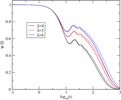
Figure 13: The density correlation function $\psi(t)$ vs. log(t) with the density-current coupling of Ref. sdd being present and $\lambda=4$. Solid line for $\Delta_{0}$ treated as a function of $\lambda$ and dashed line for $\Delta_{0}=0$.

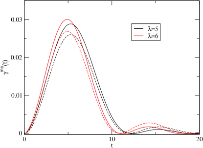
Figure 14: The cutoff function $\gamma^{mc}(t)$ vs. $t$ corresponding to results of Fig. 13. Solid and dashed lines refer to the corresponding cases of Fig. 14.

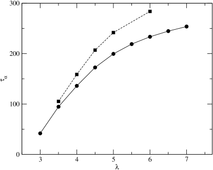
Figure 15: The relaxation time $\tau_{\alpha}$ (see text) for the density correlation function shown in Fig 13 vs. the coupling constant $\lambda$.

We present here the numerical results with $\Delta_{0}$ taken as a function of $\lambda$. Fig. 13 shows the behavior of density correlation function with time for different values of $\lambda=4$, $5$ and $6$. Solid lines. The dashed line in each case respectively represent the corresponding correlation function obtained by solving Eqn. (34) with $\Delta_{0}=0$ in Eqn. (41). Similar to Fig. 11, we plot in Fig. 14 the dependence of the cutoff functions $\gamma^{mc}$ on the parameter $\lambda$ for both of the above two cases. Solid and dashed lines show the results for $\Delta_{0}$ being given by Eqn. (42) and set to zero respectively . The correlation function relaxes slower with increasing $\lambda$. The variation of relaxation time $\tau_{\alpha}$ with the respective $\lambda$ are shown in Fig. 15 for the respective cases.

V Discussion

The slow dynamics of a deeply supercooled liquid has been studied in the past by various authors with models of generalized hydrodynamics. These models, formulated in terms coupling of slow modes in a dense liquid, are generally termed as mode coupling theory (MCT). They can be broadly divided in the following three groups.

A. The simple MCT in which an ideal ergodicity to non-ergodicity (ENE) transition is predicted. The origin of the ENE transition in basic MCT is the nonlinear coupling of density fluctuations in the pressure term of the generalized Navier-Stokes equation (12). In a simple schematic form of this model, beyond a critical value of the density dependent parameter $\lambda\geq\lambda_{c}$, the liquid undergoes a transition from the ergodic to non-ergodic state. The long time limit of the density correlation function $\psi_{\rho\rho}(t)$ is an order parameter for this ENE transition and jumps to a nonzero value beyond the transition gtze85 ; scal-jcp . This model, in various forms have been studied extensively in the literature for explaining data on glassy dynamics rmp , in particular at the initial stage of supercooling near melting point.

B. Models DM ; sdd ; gmct which takes in to account wider set of nonlinear couplings of standard hydrodynamic modes like density and currents. These nonlinearities follow from plausible generalizations of equations of hydrodynamics to short length scales. In these models the sharp ENE transition referred to in type A models is smoothed off due to mechanisms which go beyond the simple MCT. It is generally agreed that the transition of simple MCT is cut off due to such extended MCT models. It is the initial stage of viscous slow down in which types of model A are more relevant. It is also knowndas1990 that in its present form, the fully self consistent models of type B do not make the cutoff mechanism weak enough to cause large increase of time scales as seen in glassy relaxation data.

C. Extension of the simple MCT with presence of extra slow modes which are introduced from phenomenological considerations das-schilling ; yeomaj ; oppenheim1 ; biman-wolynes . The time scale of the structural relaxation in the supercooled state is linked to that of the extra slow mode which assumed to be long. Thus development of long time scales in a supercooled liquid in these models is more built in to the formulation than spontaneously coming out of the model. Both models B and C has the similarity that they reduce to model A of simple MCT when the extra couplings among hydrodynamic modes or the presence of extra slow modes are respectively ignored.

With the above background, understanding the basic mechanism of drastic slow down in structural glasses starting from the liquid side has remained a challenge. In the present work we extend the mathematical analysis of type B Models to combine with it the models of types C. First, as a test, we ignore the extra nonlinearities of type B models and consider only the pressure nonlinearity of simple MCT together with an extra slow model like that of type C models. The presence of slow diffusive process removes the ENE transition and effectively determines the final decay in the supercooled liquid as expected. The density correlation $\psi_{\rho\rho}(t)$ decays to zero. From the Fig.3 it is clear that this decay occurs increasingly slowly with decreasing $\gamma_{0}$. Second, we study the case in which the extra diffusive process is ignored i.e., $\gamma_{0}=0$. Now the results of Ref. sdd model are reproduced from our model. The present work therefore also offers a detailed mathematical deduction of models of Ref. sdd . Finally, we study the combined model of B and C. Our main finding is that in this case the decay of the density correlation is not critically controlled by the presence of the slow diffusive mode. It is the density current nonlinearities in the equations of generalized hydrodynamics which produce the dominant effect on the final decay process. The latter is determined self consistently in terms of the correlation functions and their time derivatives tran-d . We ignore transverse momentum correlations contribution to the cut off functions for simplicity and assume that they decay much faster. The dynamics is generally slower with the $\gamma_{DM}$ as compared to that with $\gamma_{SDD}$. In both case however we note that, (for the schematic cases with all wave vector dependence dropped) the ergodicity-restoring term completely wash out the slow dynamics. This means that the latter is not small enough to entail very slow dynamics.

The simple MCT predicts a ENE transition and in the so called extended MCT, the role of the nonlinearities going beyond simple coupling of density fluctuations smooths off the dynamic transition. The key factor for producing very slow dynamics lies in how the ergodicity restoring mechanism due to the the current-density couplings ($1/\rho$ nonlinearity in Eqn. (10) for ${\bf g}$) are getting suppressed. From a physical point of view, in the supercooled state the effects of currents density couplings should change in a manner so as to enhance the cage effect in the dense liquid. Whatever we call this process, be it hopping or $1/\rho$ nonlinearities, it is indeed true that the effect of this cutoff mechanism must be reduced to explain structural arrest from the liquid side within MCT. The present work in fact puts a constraint of similar nature on the phenomenological models that have been proposed in recent literature to serve this. Going beyond MCT, various scenarios have been proposed in this respect, including spontaneous breakdown of ergodicity remi and Random first order transition wolynes-rfot to explain this structural arrest along the lines of Adam and Gibbs classic papers. However coming from the liquid side, using a microscopic approach like MCT, this still remains an open problem.

Appendix A Renormalization

The key quantity which determined the renormalization of the correlation function matrix from ${\bf G}_{0}$ to ${\bf G}$, is the self energy matrix $\Sigma$. This is expressed in the Dyson equation (27). There are primarily two types of elements $\Sigma_{\psi\hat{\psi}}$ and $\Sigma_{\hat{\psi}\hat{\psi}}$ respectively referred to as response and correlation type matrix elements. Let us first consider the Dyson equation for the case in which both indices in the matrix Eqn. (27) correspond to the un-hatted fields. In this case, we have for the two respective terms on the right hand side,

• $[{\bf G_{0}}^{-1}]_{\alpha\beta}=0$ which follows from the action (II.2) obtained in the MSR field theory.

• ${\bf\Sigma}_{\alpha\beta}=0$ which follows from causal nature of the response functions in MSR field theory.

We therefore obtain that the elements of the ${\bf G}^{-1}$ matrix corresponding to the un-hatted fields, ${\left[{\bf G}^{-1}\right]}_{\alpha\beta}=0$. The inverse of the green function matrix ${\bf G}$ is obtained in the following block diagonal form

$${\bf G}^{-1}=\left[\begin{array}[]{cc}\bigcirc&{\cal R}^{{\dagger}}\\ {\cal R}&{\cal C}\\ \end{array}\right]$$ (43)

The renormalized for of the matrix ${\cal R}$ and ${\cal C}$ are obtained in terms of the elements of the self energy matrix $\Sigma$ introduced in the Dyson equation (27). Here the symbol ${\cal R}^{{\dagger}}$ denotes the hermitian conjugate of ${\cal R}$. By taking out the leading order wave number dependence of the respective correlation and response self energies, we define the various elements of $\gamma_{\psi\hat{\psi}}$ where $\psi{\in}\{\rho,{\bf g}\}$. The renormalized elements of the matrix ${\cal R}$ and ${\cal C}$ are respectively listed in table 2 and 3 . The above matrix elements for ${\bf G}^{-1}$ are obtained from renormalizing the corresponding zeroth order contributions in ${\bf G}_{0}^{-1}$ with the appropriate self energies. The $c$, $\gamma$ and ${L}$ respectively denote the renormalized quantities for the sound speed $c_{0}$, the diffusion constant $\gamma_{0}$, and the longitudinal viscosity $\tilde{L}_{ij}^{0}$.

$$c^{2}(q,\omega) = c_{0}^{2}+\gamma_{\hat{g}\rho}({\bf q},\omega)$$

$$\gamma({\bf q},\omega) = \gamma_{0}+i{\gamma_{\hat{\rho}\rho}({\bf q},\omega)}$$

$$L_{ij}({\bf q},\omega) = \tilde{L}_{ij}^{0}+i\Sigma_{\hat{g}_{i}{g}_{j}}({\bf q},\omega)~{}~{}.$$

The contribution to $\gamma_{\hat{\rho}{g}}$ is taken at the lowest order $O(q^{2})$. Inverting the matrix ${\bf G}^{-1}$ having the above structure (43), we obtain for the correlation functions of the physical, un-hatted field variables

$$G_{\alpha\beta}=-\sum_{\mu\nu}G_{\alpha\hat{\mu}}C_{\hat{\mu}\hat{\nu}}G_{\hat{\nu}\beta}$$ (44)

where Greek letter subscripts take values $\rho,{\bf g}$, and the self energy matrix $\Sigma_{\hat{\mu}\hat{\nu}}$ determine the corresponding elements of the matrix ${\cal C}$. From the set of equations denoted by (27) we also obtain that the response functions $G_{\alpha\hat{\mu}}$. Here we make use of the functional identity,

$$\int D(\psi)\frac{\delta}{\delta\psi_{\hat{\alpha}}(1)}\left[\psi_{\beta}(2){e}^{-{\cal A}[\psi]}\right]=0\$$

where $D(\psi)$ denotes the functional integral with the fields $\{\psi\}$ and ${\cal A}$ is the MSR action ( for example see Eqn. II.2) ) with respect to which averaged are obtained. Using this identity we obtain

$$\left[(G_{0}^{-1})_{\hat{\alpha}\mu}(13)-\Sigma_{\hat{\alpha}\mu}(13)\right]G_{\mu\hat{\beta}}(32)=\delta(12)\delta_{\hat{\alpha}\hat{\beta}}~{}~{}.$$ (45)

The self energies $\Sigma_{\hat{\alpha}\mu}$ are expressed in a perturbation theory in terms of the two-point correlation and response functions. Now inverting the matrix ${\cal R}$ given in table 2, we obtain the response function in the following form.

$$G_{\alpha\hat{\mu}}=\frac{N_{\alpha\hat{\mu}}}{\cal D}$$ (46)

where the matrix $N$ is given in table 4. The determinant ${\cal D}$ in the denominator of Eqn. (46) is given by.

$${\cal D}=(\omega+iq^{2}\gamma)~{}(\omega+iq^{2}{L})-q^{2}c^{2}~{}~{}.$$ (47)

$L(q,\omega)$ is the renormalized longitudinal viscosity obtained in terms of the self energy matrix:

$$L({\bf q},\omega)=\tilde{L}_{0}+i\gamma_{\hat{g}{g}}({\bf q},\omega)~{}~{}.$$

The bare longitudinal viscosity is obtained as $L_{0}=(\zeta_{0}+4\eta_{0}/3)$ and the corresponding kinematic viscosity $\tilde{L}_{0}$ in Eqn. (A) is denoted as $\tilde{L}_{0}=L_{0}/\rho_{0}$.

The symmetries of the vector field ${\bf g}$ and the scaler field $\rho$ require that the vertices having the corresponding MSR hatted field $\hat{g}_{i}$ or $\hat{\rho}$ are associated with a factor of $q$, due to the total derivatives present in the nonlinearities in the respective FNH equations. Using this, we first estimate the leading order wave vector dependence of the various self energy functions. The correlation self energy, elements between two hatted fields are obtained as

$$\Sigma_{\hat{g}_{i}\hat{g}_{j}}({\bf q},\omega) = -q^{2}\gamma_{\hat{g}_{i}\hat{g}_{j}}(0,\omega)$$ (48)

$$\Sigma_{\hat{\rho}\hat{\rho}}({\bf q},\omega) = -q^{2}\gamma_{\hat{\rho}\hat{\rho}}(0,\omega)$$ (49)

$$\Sigma_{\hat{\rho}\hat{g}_{i}}({\bf q},\omega) = -q^{3}\gamma_{\hat{\rho}\hat{g}_{i}}(0,\omega)$$ (50)

On the other hand the response self energy elements between hatted and un-hatted fields $\Sigma_{\psi\hat{\psi}}$ generally satisfies the condition

$$\Sigma_{\psi\hat{\psi}}({\bf q},\omega)=-\Sigma^{*}_{\hat{\psi}{\psi}}({\bf q},\omega)$$ (51)

The leading order behavior of the response self energy elements are obtained as

$$\Sigma_{\hat{g}_{i}{g}_{j}}({\bf q},\omega) = -iq^{2}\gamma_{\hat{g}_{i}{g}_{j}}(0,\omega)$$ (52)

$$\Sigma_{\hat{\rho}\rho}({\bf q},\omega) = -iq^{2}\gamma_{\hat{\rho}\rho}(0,\omega)$$ (53)

$$\Sigma_{\hat{g}_{i}\rho}({\bf q},\omega) = -iq^{3}\gamma_{\hat{g}_{i}\rho}(0,\omega)$$ (54)

$$\Sigma_{\hat{\rho}{g}_{i}}({\bf q},\omega) = -iq^{3}\gamma_{\hat{\rho}{g}_{i}}(0,\omega)$$ (55)

We find that at the one loop order, for the self energies on the right hand side of Eqns. (54)-(55), the $O(q)$ contribution is vanishing. In a similar way the total contribution to the self energy $\gamma_{\hat{\rho}{g}}$ from the one loop diagrams involving the nonlinearity in the continuity equation is of $O(q^{2})$. The latter therefore is ignored compared to 1 in the matrix element $N_{\rho\hat{g}}$ shown in table 4. These diagrams are explicitly shown at the end of this section. Using the above forms for the self energies in the fluctuation dissipation relations (23)-(24) and doing a leading order analysis in the hydrodynamic limit, we obtain a set of useful relations between the correlation and response self energies. These relations are essential in demonstrating that the theory is renormalizable in terms of a redefined quantities presented in Eqns. (A)-(A), in terms of the self energy functions. Doing a standard analysis DM of the expression (44) for the correlation functions, the following self-energy relations are obtained in the hydrodynamic limit

$$\gamma_{\hat{g}\hat{g}} = 2~{}\beta^{-1}\rho_{0}\gamma^{\prime}_{\hat{g}g}$$ (56)

$$\gamma_{\hat{\rho}\hat{\rho}} = -2~{}\beta^{-1}\frac{\rho_{0}}{c^{2}_{0}}\gamma^{{}^{\prime}}_{\hat{\rho}\rho}~{}~{}.,$$ (57)

where the prime indicates the real part of the corresponding self energy element. The renormalized viscosity is given by either in terms of the response or the correlation self energies. We write

$$L=L_{0}+\frac{\beta}{2}\gamma_{\hat{g}\hat{g}}~{}~{}.$$ (58)

Similarly the renormalized diffusion coefficient is given by

$$\gamma=\gamma_{0}+\frac{\beta}{2}\frac{c^{2}_{0}}{\rho_{0}}\gamma_{\hat{\rho}\hat{\rho}}$$ (59)

A.1 One loop contribution for $\Sigma_{\hat{\rho}g}$

The contribution to the first diagram ( see Fig. 16 ) for $\Sigma_{\hat{\rho}{g}}$ as shown in Fig. 16 is obtained as

$$\Sigma_{\hat{\rho}g}^{(1)}(q,t)=\frac{q}{\rho_{0}^{2}}\int\frac{d{\bf k}}{(2\pi)^{3}}u(q-uk)~{}G_{\rho\hat{\rho}}(q-k,t)~{}G_{g\rho}(k,t)~{}~{}.$$ (60)

$u$ is the cosine of the angle between ${\bf q}$ and ${\bf k}$. For the second diagram shown in the same figure we obtain

$$\Sigma_{\hat{\rho}{g}}^{(2)}(q,t)=\frac{q}{\rho_{0}^{2}}\int\frac{d{\bf k}}{(2\pi)^{3}}u^{2}k~{}G_{\rho\rho}(q-k,t)~{}G_{g\hat{\rho}}(k,t).$$ (61)

We use the Fluctuation-dissipation relation

$$i\Theta(t)G_{\beta\rho}(q,t)=\beta^{-1}\chi_{\rho\rho}G_{\beta\hat{\rho}}(q,t),$$ (62)

where $\Theta(t)$ is the Heaveside step function. We obtain for the total contribution from the sum of the two diagrams as,

$$\Sigma_{\hat{\rho}{g}}(q,t) = \Sigma_{\hat{\rho}g}^{(1)}(q,t)+\Sigma_{\hat{\rho}g}^{(2)}(q,t)$$ (63)

$$= i\Theta(t)~{}q^{2}\frac{\beta c^{2}}{\rho_{0}^{2}}\int\frac{d{\bf k}}{(2\pi)^{3}}\Big{(}u~{}G_{\rho\rho}(q-k,t)~{}G_{g\rho}(k,t)\Big{)}~{}~{}.$$

Figure 1: One loop contributions to $\Sigma_{{\hat{g}}_{i}{\hat{g}}_{j}}$.

Figure 2: One loop contributions to $\Sigma_{\hat{\rho}\hat{\rho}}$.

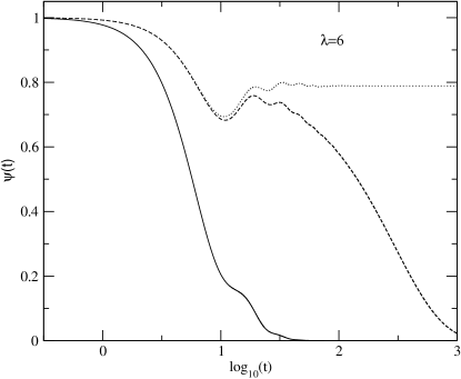
Figure 5: The density correlation function $\psi(t)$ Vs. log(t) for the thermodynamic parameter $\lambda=6$ and $\Delta_{0}=0$. With the cutoff function $\gamma^{mc}$(see text) set to a) zero(dotted), b) $\gamma_{SDD}$(solid), and c) $\gamma_{DM}$ (dashed).

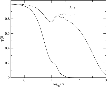
Figure 6: The density correlation function $\psi(t)$ Vs. log(t) for the thermodynamic parameter $\lambda=8$ and $\Delta_{0}=0$. With the cutoff function $\gamma^{mc}$(see text) set to a) zero(dotted), b) $\gamma_{SDD}$(solid), and c) $\gamma_{DM}$ (dashed).

Figure 16: One loop contributions to $\Sigma_{\hat{\rho}g}$.

References

- (1) E. Leutheusser, Phys. Rev. A, 29, 2765 (1984).
- (2) U. Bengtzelius, W. Gőtze, and A. Sjőlander, J. Phys. C 17, 5915 (1984).
- (3) U. Bengtzelius, and A. Sjőlander, Annals of New York Acad. of Sc. 484, 229 (1986).
- (4) S. P. Das, Statistical Physics of Liquids at Freezing and Beyond (Cambridge University Press, NewYork, 2011).
- (5) K. Kawasaki, J. Stat. Phys. 110, 1249 (2003).
- (6) U. Harbola and S. P. Das, Physical Review E 65, 036138 (2003).
- (7) C. Kaur, and S.P. Das, Physical Review Letters 89, 085701 (2002).
- (8) L. A. Turski, Physica Scripta T 13, 259 (1986).
- (9) A. Sjőlander, Physica Scripta 32, 314 (1985).
- (10) S. P. Das, and J. W. Dufty Physical Review 46, 6371 (1992).
- (11) S. P. Das and G.F. Mazenko, Phys. Rev. A 34, 2265 (1986).
- (12) G. F. Mazenko, and J. Yeo, J. Statist. Phys. 74, 1017 (1994).
- (13) R. Schimitz, J. W. Dufty, and P. De, Phys. Rev. Lett.71, 2066 (1993).
- (14) R. Kree and A. Zippelius L. A. Turski, Phys. Rev. Lett. 58, 1656 (1987).
- (15) A. Sjőlander, L. A. Turski, J. Phys. C (Solid State) 11,1973 (1978).
- (16) S. Dattagupta, and L. A. Turski, Phys. Rev. Lett. 54, 2359 (1985).
- (17) S. Dattagupta, and L. A. Turski, Phys. Rev.E 47, 1222 (1993).
- (18) S. M. Bhattacharyya, B. Bagchi, and P. G. Wolynes, Phys. Rev. E 72, 031509 (2005).
- (19) C. Z. Liu, and I. Oppenheim, 1997, Physica A 235, 369 (1997).
- (20) M. Manno, and I. Oppenheim, Physica A 265, 520 (1999).
- (21) S. Srivastava, and S. P. Das Physics Letters A 286, 76 (2001).
- (22) W. Gőtze, and L. Sjőgren, Transp. Theory Stat. Phys. 24, 801 (1995).
- (23) S. P. Das, Rev. Mod. Phys. 76, 785 (2004).
- (24) S. P. Das, and R. Schilling, Phys. Rev. E 50, 1265 (1994).
- (25) C. P. Enz, L. A. Turski, Physica A 96, 369 (1979).
- (26) A. Thellung, Physica 19, 217, (1953).
- (27) L. A. Turski, Physica A 57 432 (1972).
- (28) L. A. Turski, Phys. Rev. A 30, 2779 (1984)
- (29) S. K. Ma, and G. F. Mazenko, Phys. Rev. B 11, 4077 (1975).
- (30) J. S. Langer, and L. Turski, Phys. Rev. A 8, 3230 (1973).
- (31) J.-P. Hansen, and I. R. McDonald, Theory of Simple Liquids, New York: Academic Press, 1986.
- (32) I. Dzyaloshinskii, and G. Volovick, Ann. Phys. (N.Y.) 125, 67 (1980).
- (33) S. P. Das, G. F. Mazenko, S. Ramaswamy, and J. Toner, Phys. Rev. Lett. 54, 118(1985).
- (34) S. P. Das, Phys. Rev. E 54, 1715 (1996).
- (35) K. Kawasaki and S. Miyazima, Z. Phys. B, Condensed Matter, 103, 423 (1997).
- (36) T. Munakata, Aust. J. Phys. 49, 25 (1996).
- (37) D. S. Dean, J Phys. A : Math. Gen. 29 L613 (1996).
- (38) P. C. Martin, E. D. Siggia, and H. A. Rose, Phys. Rev. A 8,423 (1973).
- (39) R. V. Jensen, J. Statist. Phys. 25, 183 (1981).
- (40) R. Bausch, H. Janssen, and H. Wagner, Z. Phys. B 24, 113 (1976).
- (41) H. C. Andersen, J. Phys. Chem. B 106, 8326 (2002).
- (42) H. C. Andersen, J. Phys. Chem. B 107, 10226 (2003).
- (43) H. C. Andersen, J. Phys. Chem. B 107, 10234 (2003).
- (44) A. Andreanov, G. Biroli, and A. Lefevre, J. Stat. Mech, P07008 (2006).
- (45) S. P. Das and G. F. Mazenko, Phys. Rev. E. 79, 021504 (2009).
- (46) S. P. Das and G. F. Mazenko, Journal of Statistical Physics 152, 159 (2013).
- (47) G. F. Mazenko, Nonequilibrium Statistical Mechanics, New York: Wiley-VCH, 2006
- (48) I. de Schepper, A. F. E. M. Haffmans, and H. van Beijeren, Phys. Rev. Lett. 57, 1715 (1986)
- (49) S. P. Das, The Journal of chemical physics 105, 8822 (1996).
- (50) W. Gőtze, Z. Phys. B: Condens. Matter 60, 195 (1985).
- (51) S. P. Das, The Journal of chemical physics 98, 3328 (1993).
- (52) G. Biroli, J. Bouchard, K.Miyazaki, and D. R. Reichman, Phys. Rev. Lett. 97, 195701 (2006).
- (53) S. P. Das, Phys. Rev. A 36, 211 (1987); ibid, Phys. Rev. A 42, 6116 (1990).
- (54) Ideal MCT shows that the transverse current correlation changes from diffusive to propagating modes representing shear waves in an amorphous solid. In some works, hydrodynamic description of the glassy systems is extended to include this property even at the linear order fluctuations assuming that fluid particles freeze over an amorphous lattice. However, glassy states are not with long range order and strictly there is no new Goldstone mode in the system. Nevertheless such models with transverse sound modes have been used in studying glassy dynamics. It is important to note our reference to longitudinal current coupling in the cut off mechanism is beyond simple MCT. Our analysis shows that correlation of longitudinal current in a compressible liquid couples to density correlation plays a key role in deciding the strength of the cutoff mechanism.
- (55) R. Monasson, Phys. Rev. Lett. 75, 2847 (1995).
- (56) T. R. Kirkpatrick, D. Thirumalai, and P. G.Wolynes, Phys. Rev. A 40, 1045 (1989).