Far-Infrared Dust Temperatures and Column Densities of the MALT90 Molecular Clump Sample

Abstract

We present dust column densities and dust temperatures for $\sim 3000$ young high-mass molecular clumps from the Millimetre Astronomy Legacy Team 90 GHz (MALT90) survey, derived from adjusting single temperature dust emission models to the far-infrared intensity maps measured between 160 and 870 µm from the Herschel/Hi-Gal and APEX/ATLASGAL surveys. We discuss the methodology employed in analyzing the data, calculating physical parameters, and estimating their uncertainties. The population average dust temperature of the clumps are: $16.8\pm 0.2$ K for the clumps that do not exhibit mid-infrared signatures of star formation (Quiescent clumps), $18.6\pm 0.2$ K for the clumps that display mid-infrared signatures of ongoing star formation but have not yet developed an Hii region (Protostellar clumps), and $23.7\pm 0.2$ and $28.1\pm 0.3$ K for clumps associated with Hii and photo-dissociation regions, respectively. These four groups exhibit large overlaps in their temperature distributions, with dispersions ranging between 4 and 6 K. The median of the peak column densities of the Protostellar clump population is $0.20\pm 0.02$ gr cm^-2, which is about 50% higher compared to the median of the peak column densities associated with clumps in the other evolutionary stages. We compare the dust temperatures and column densities measured toward the center of the clumps with the mean values of each clump. We find that in the Quiescent clumps the dust temperature increases toward the outer regions and that they are associated with the shallowest column density profiles. In contrast, molecular clumps in the Protostellar or Hii region phase have dust temperature gradients more consistent with internal heating and are associated with steeper column density profiles compared with the Quiescent clumps.

1 INTRODUCTION

Most of the star formation in the Galaxy occurs in clusters associated with at least one high-mass star (Adams, 2010). An understanding of star formation on global galactic and extra-galactic scales therefore entails the study of the early evolution of high-mass stars and how they impact their molecular environment.

The physical characterization of the places where high-mass stars form is an important observational achievement of the far-infrared (far-IR) and submillimeter astronomy of the last decades. High-mass stars form in massive molecular clumps of sizes $\lesssim 1$ pc, column densities $\gtrsim 0.1$ gr cm^-2, densities $n_{\rm H_{2}}\gtrsim 10^{4}$ cm^-3, and masses $>200$  $M_{\odot}$ (Tan et al., 2014), with temperatures depending on their evolutionary stage. Determining the evolutionary sequence of these massive molecular clumps and their properties is currently an active field of study. We can define a schematic timeline that comprises four major observational stages (Jackson et al., 2013; Chambers et al., 2009):

1. Quiescent and prestellar sources, that is, molecular clumps in the earliest phase with no embedded high-mass young stellar objects (HMYSOs). Some of these clumps are called infrared dark clumps (IRDCs) because they appear in absorption against the bright mid-IR background associated with the Galactic plane.

2. Protostellar clumps are those associated with signs of star formation such as outflows and HMYSOs, but where Hii regions have not developed. We expect the embedded young high-mass stars to accrete at a high rate ($\geq 10^{-4}$  $M_{\odot}$ yr^-1, e.g., McKee & Tan, 2003; Keto & Wood, 2006; Tan et al., 2014) and to reach the main sequence in typically $\lesssim 10^{5}$ yr (Behrend & Maeder, 2001; Molinari et al., 2008). Based on the Kelvin-Helmholtz contraction timescale, high-mass young stars will be likely on the main sequence while still accreting.

3. Molecular clumps associated with compact Hii regions. The young high-mass stars in these clumps have probably finished their main accretion phase and have reached their final masses. Strong UV radiation from the newly born high-mass stars start to ionize the surrounding cocoon.

4. Clumps in a late evolutionary stage, where the ionizing radiation, winds and outflows feedback, and the expansion of the ionized gas finally disrupt the molecular envelope, marking the transition to an observational stage characterized by an extended classical Hii region and a photodissociation region (PDR).

Studying the dust continuum emission in the mid-IR, far-IR, and submillimeter range is one of the most reliable ways to determine the evolutionary phase of molecular clumps. Dust emission in the submillimeter is usually optically thin and traces both cold and warm environments. By combining large infrared Galactic plane surveys like Hi-GAL (Herschel Infrared Galactic plane survey, Molinari et al., 2010), ATLASGAL (APEX Telescope Large Area Survey of the Galaxy, Schuller et al., 2009), GLIMPSE (Galactic Legacy Infrared Midplane Survey Extraordinaire, Benjamin et al., 2003), and MIPSGAL (Carey, 2008), we can determine the evolutionary state and calculate basic physical parameters of a large sample of molecular clumps.

With this prospect in mind, the Millimeter Astronomy Legacy Team 90 GHz (MALT90) survey (Rathborne et al. in preparation; Jackson et al., 2013; Foster et al., 2011, 2013) has studied 3246 molecular clumps identified using SExtractor (Bertin & Arnouts, 1996) from the ATLASGAL data at 870$\mu$m (Contreras et al., 2013; Urquhart et al., 2014a). MALT90 has mapped these clumps in 15 molecular and one hydrogen recombination line located in the 90 GHz atmospheric band using the 22 m Mopra telescope. The objective is to determine the main physical and chemical characteristics of a statistically relevant sample of high-mass molecular clumps over a wide range of evolutionary stages. Approximately 80% of the MALT90 sources exhibit mid-IR characteristics that allow us to classify them into one of the four preceding evolutionary stages: Quiescent, Protostellar, Hii region, or PDR. This classification of the sources was done by visual inspection of Spitzer images at 3.6, 4.5, 8.0, and 24 µm, as described in Hoq et al. (2013) (see also Foster et al., 2011). By combining the MALT90 dataset with far-IR continuum and molecular line data, we can characterize quantitatively their temperatures, column densities, volume densities, distances, masses, physical sizes, kinematics, luminosity, and chemistry of the clumps.

In this paper, we focus on the dust continuum emission of the MALT90 molecular clump sample. We model the far-IR and submillimeter emission to derive physical parameters which, to a first approximation, are distance independent such as the dust temperature and the column density. Forthcoming publications by Whitaker et al. (in preparation) and Contreras et al. (in preparation) will present kinematic distances and analyze the clumps’ masses, sizes, volume densities, and luminosities. Preliminary analysis of the molecular emission indicates that the relative abundances, line opacities (Rathborne et al., in preparation, see also Hoq et al., 2013), and infall signatures (Jackson et al., in preparation) are consistent with the mid-IR classification acting as a proxy for clump evolution. The MALT90 data have been already used in several other studies of high-mass star formation, either based on a small ($<10$) set of relevant sources (Rathborne et al., 2014; Stephens et al., 2015; Walker et al., 2015; Deharveng et al., 2015) or using a statistical approach on a larger sample ($>30$, Hoq et al., 2013; Miettinen, 2014; Yu & Wang, 2015; He et al., 2015). In these studies with large samples (with the exception of Hoq et al., 2013), the dust temperature and column density of the clumps have not been simultaneously derived from a model of the far-infrared spectral energy distribution (SED). This paper aims to complement future high-mass star formation studies based on the MALT90 sample by supplying robust measurements of these physical properties and their uncertainties.

Section 2 of this work presents the main characteristics of the data set and its reduction. Section 3 describes the methods used for analyzing the data, the modeling of the dust emission, and uncertainty and degeneracy estimations. Section 4 discusses possible interpretations of the statistical results of the dust parameters and, specially, how the clump evolutionary stages correlate with the dust derived physical parameters. Section 5 summarizes the main results of this work.

2 OBSERVATIONS

The analysis presented in this work is based on data taken with the Herschel Space Observatory (HSO, Pilbratt et al., 2010) and with the APEX telescope (Güsten et al., 2006).

2.1 Processing of Public HSO Hi-GAL Data

We use public HSO data from the Herschel Infrared Galactic Plane Survey key-project (Hi-GAL, Molinari et al., 2010) observed between January of 2010 and November of 2012 and obtained from the Herschel Science Archive. The observations were made using the parallel, fast-scanning mode, in which five wavebands were observed simultaneously using the PACS (Poglitsch et al., 2010) and the SPIRE (Griffin et al., 2010) bolometer arrays. The data version obtained from the Herschel Science Archive corresponds to the Standard Product Generation version 9.2.0.

Columns 1 to 4 of Table 1 list the instrument, the representative wavelength in microns of each observed band, the angular resolution represented by the FWHM of the point spread function (Olmi et al., 2013), and the estimated point source sensitivity ($\sigma_{p}$), respectively. The point source sensitivity, assuming Gaussian beams, is given by $\sigma_{\rm rms}\Omega_{b}\left(\Omega_{b}/2\Omega_{\rm pix}\right)^{-1/2}$, where $\sigma_{\rm rms}$ is the rms variations in intensity units, $\Omega_{b}$ is the beam solid angle, and $\Omega_{\rm pix}$ is the pixel solid angle. The fifth column gives the noise level of the convolved and re-gridded maps (see Sections 3.1 and 3.2) and the sixth column lists the observatory where the data were taken. Throughout this work, we will refer to the data related to a specific waveband by their representative wavelength in micrometers. The position uncertainty of the Hi-GAL maps is $\sim$3″.

The generation of maps that combine the two orthogonal scan directions was done using the Herschel Interactive Processing Environment (HIPE) versions 9.2 and 10. Cross-scan combination and destriping were performed over 42 Hi-GAL fields of approximately $2\fdg 2\times 2\fdg 2$ using the standard tools available in HIPE. Columns 1 to 4 of Table 2 give the target name, the ID of the observation, the observing mode, and the observation dates, respectively. For the SPIRE maps, we applied the extended source calibration procedure (Section 5.2.5 from the SPIRE Handbook) since most of MALT90 sources correspond to dense clumps that are comparable to or larger than the largest SPIRE beam size. The saturation limit of the nominal mode for SPIRE (Section 4.1.1 from the SPIRE Handbook) is approximately 200 Jy beam^-1. To prevent saturation, fields with longitudes $|l|\leq 5$° were observed with SPIRE using the bright observing mode instead of the nominal observing mode.

2.2 Other HSO Data

In addition to Hi-GAL data, we used data from three observations made using the SPIRE bright mode by the HOBYS key project (Herschel Imaging Survey of OB YSOs, Motte et al., 2010). Table 2 lists these observations’ IDs. They were directed toward the NGC 6334 ridge and the central part of M17, areas which are heavily saturated in the Hi-GAL data.

2.3 ATLASGAL Archival Data

Data at 870 $\mu$m were taken between 2007 and 2010 using the bolometer LABOCA (Siringo et al., 2009) installed on the APEX telescope located in Chajnantor valley, Chile, as part of the ATLASGAL key project (Schuller et al., 2009). Calibrated and reduced fits images were obtained from the data public releases made by Contreras et al. (2013) and Urquhart et al. (2014a). Table 1 displays the angular resolution, the point source sensitivity calculated as in Section 2.1 using $\sigma_{\rm rms}=60$ mJy beam^-1 and $\Omega_{b}/\Omega_{\rm pix}=11.6$ (Contreras et al., 2013), and the typical noise of the convolved and re-gridded ATLASGAL maps. In addition to this noise, we assume a 10% uncertainty in the absolute calibration.

3 ANALYSIS

The following sections describe the methods used in the model fitting and uncertainty estimations. There are 2573 ATLASGAL sources observed by MALT90 classified according to their mid-IR appearance as Quiescent, Protostellar, Hii region, or PDR. The remaining sources (673) exhibit no clear mid-IR features that allow us to classify them unambiguously in these evolutionary stages. We refer to these sources as “Uncertain.” The MALT90 catalog includes 3557 entries, of which 2935 sources are associated with molecular emission detected at a single V_LSR. MALT90 also detected molecular emission arising at two V_LSR toward 311 ATLASGAL sources, which correspond to 622 entries in the MALT90 catalog. The continuum emission from these sources comes from two or more clumps located at different distances, complicating the interpretation. We have calculated column densities and temperatures toward these blended sources, but we have excluded them from the discussion of Section 4.

3.1 Noise Estimation of the HSO Data

To a first approximation, the intensity assigned to each pixel is given by the average of the bolometer readings that covers that pixel position. The spatial sampling of the maps, on the other hand, includes $\sim$3 pixels per beamwidth. Observed astronomical signals vary spatially on angular scales $\gtrsim$ 1 beamsize. Therefore, in the large fraction of the map area that is away from very strong sources, we expect that the differences between adjacent pixels are dominated by instrumental noise. In order to estimate this noise, we use the high-pass filter defined by Rank et al. (1999) to determine the distribution of pixel-to-pixel variations and filter out astronomical emission. The width of this distribution determines the typical noise through the relation $2.36\sigma=\text{FWHM}$. The advantage of this method is that it gives us an extra and relatively simple way to estimate the noise of the final maps. The noise estimation is similar to that obtained from jackknife maps, produced by taking the difference between maps generated by the two halves of the bolometer array (see Nguyen et al., 2010, for an analogous procedure).

The 1-$\sigma$ point source sensitivities derived from the high-pass filter method described above are typically 18 and 24 mJy for the two PACS bands at 70 and 160 µm, and 12 mJy for the three SPIRE bands at 250, 350, and 500 µm. These derived sensitivities are in good agreement with the ones expected for the Hi-GAL survey (Molinari et al., 2010) and in reasonable agreement with the sensitivities expected for the parallel mode, with the possible exception of the 160 $\mu$m band where we estimate about half of the expected noise. The noise value derived at 250 $\mu$m is comparable with the noise component derived by Martin et al. (2010) also from Hi-GAL data, indicating that our estimation effectively filters most of the sky emission variations, including the cirrus noise. Finally, and as expected, we find that the noise in fields observed in the SPIRE bright mode is $\sim$4 times larger compared to that in fields observed in nominal mode. For subsequent analyses, we consider an additional independent calibration uncertainty of 10% whenever we compare data among different bands, as for example, in the SED fitting. This 10% represents a conservative approximation of the combined calibration uncertainty of the SPIRE photometers (5.5%) and the beam solid angle (4%, see Section 5.2.13 of the SPIRE Handbook).

3.2 Convolution to a Common Resolution and Foreground/Background Filtering

Multi-wavelength studies of extended astronomical objects, such as star-forming clumps and IRDCs, often combine data taken with different angular resolutions. Therefore, to make an adequate comparison of the observed intensities, it is necessary to transform the images to a common angular resolution. We accomplish this by convolving the images to the lowest available resolution, given by the 500 µm SPIRE instrument, using the convolution kernels of Aniano et al. (2011) in the case of HSO data. The ATLASGAL data were convolved by a two-dimensional Gaussian with FWHM equal to $\sqrt{35\farcs 0^{2}-19\farcs 2^{2}}\approx 29\farcs 3$, under the assumption that the point spread functions of the ATLASGAL and the 500 µm data are Gaussians. In addition, to compare the intensity of the HSO images with that of the APEX telescope, we need to remove from the HSO data the low spatial frequency emission that has been filtered from the ATLASGAL images. The ATLASGAL spatial filtering is performed during the data reduction, and is a by-product of the atmospheric subtraction method which removes correlated signal between the bolometers (Siringo et al., 2009). As a consequence, any uniform astronomical signal covering spatial scales larger than 2$\farcm$5 is lost (Schuller et al., 2009).

We filter the HSO data in a similar way by subtracting a background image from each field and at each band. We assume that this background is a smooth additive component that arises from diffuse emission either behind or in front of the clump. In addition to filtering the HSO data in order to combine it with ATLASGAL, the background subtraction serves two more purposes: it separates the Galactic cirrus emission from the molecular clouds (e.g., Battersby et al., 2011), and it corrects for the unknown zero level of the HSO photometric scale. Our background model consists of a lower-envelope of the original data under two constrains: its value at each pixel has to be less than in the image, within a 2-$\sigma$ tolerance, and it has to vary by less than 10% over 2$\farcm$5, which corresponds to the ATLASGAL filter angular scale.

We construct a background image for each Hi-GAL field following a slight modification of the CUPID-findback algorithm of the Starlink suite (Berry et al., 2013). The iterative algorithm used to construct the background starts with the original image. Then, we calculate a smoothed image by setting to zero (in the Fourier transform plane) the spatial frequencies corresponding to flux variations on angular scales $<2\farcm 5$. For each pixel in this smoothed image with a value larger than the corresponding pixel in the original image plus $2\sigma$, the pixel value from the smoothed image is replaced by the one in the original image, where $\sigma$ is the uncertainty of the map. The remaining pixels in the smoothed image are kept unchanged. The resultant map is the first iteration of the algorithm. This first iteration replaces the starting image and the cycle repeats, generating further iterations, until the change between two consecutive iterations is less than 5% in all pixels.

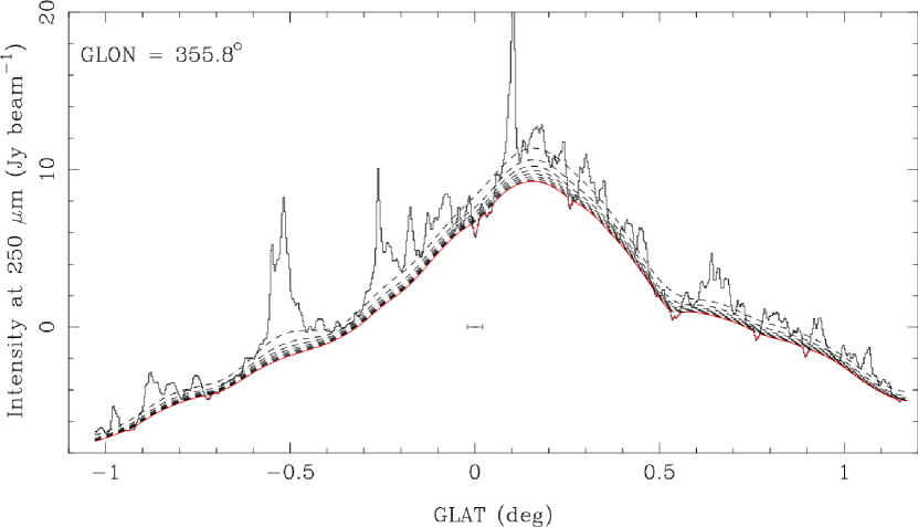
Figure 1: 250 $\mu$m intensity measured across the Galactic plane at longitude $l=355\fdg 8$. The dashed lines show the intermediate iterations of the background subtraction algorithm and the red line the final adopted background, which is a smooth lower envelope of the original data. The bar located at $b=0\arcdeg$ and Intensity$=0$ Jy beam^-1 marks the shortest angular scale filtered by the background, that is, 2$\farcm$5. Note the negative values of the intensity are due to the arbitrary zero-level of the HSO photometry scale.

Figure 1 shows an example of this process, which converges to a smooth lower-envelope of the original image. The solid black line shows a cut along $l=355\fdg 8$ of the intensity measured at 250 $\mu$m. Negative intensity values away from the Galactic plane are a consequence of the arbitrary zero-level of the HSO photometry scale. Dashed lines show different iterations of the algorithm and the final adopted background is marked in red. The error bar at the center of the plot measures 2$\farcm$5, that is, the shortest angular scale filtered by the background. Note that Figure 1 shows a cut across latitude at a fixed longitude, but the algorithm works on the two-dimensional image, not assuming any particular preferred direction.

3.3 Single Temperature Grey-Body Model

We interpret the observed intensities as arising from a single temperature grey-body dust emission model. The monochromatic intensity at a frequency $\nu$ is given by

$$I_{\nu}(T_{d},N_{g})=B_{\nu}(T_{d})\left(1-e^{-\tau_{\nu}}\right)~{}~{},$$ (1)

where $B_{\nu}(T_{d})$ is the Planck function at a dust temperature $T_{d}$ and

$$\tau_{\nu} =N_{\rm dust}\kappa_{\nu}~{}~{},$$ (2)

$$={\rm GDR}\times N_{g}\kappa_{\nu}~{}~{},$$ (3)

where $\tau_{\nu}$ is the dust optical depth, $N_{\rm dust}$ is the dust column density, and $\kappa_{\nu}$ is the dust absorption coefficient. The relation between the dust and gas ($N_{g}$) column densities is determined by the gas-to-dust mass ratio (GDR), which we assume is equal to $100$. We also define the particle column density by $N_{p}:=N_{g}/(\mu m_{\rm H})$, where $\mu=2.3$. The number column density of molecular hydrogen ($N_{\rm H_{2}}$) is obtained in the same way but using $\mu=2.8$ (Kauffmann et al., 2008), under the assumption that all the hydrogen is in molecular form. We assume throughout this work that $N_{g}$ is measured in gr cm^-2 and $N_{\rm H_{2}}$ and $N_{p}$ in cm^-2. To compare the dust emission model to the data, we weight the intensity given by Equation (1) by the spectral response function of the specific waveband, in order to avoid post-fitting color corrections (see for example, Smith et al., 2012).

We exclude the 70 µm intensity from the single $T_{d}$ fitting since this emission cannot be adequately reproduced by Equation (1) (see Section 3.4). This problem has been noted by several authors (e.g., Elia et al., 2010; Smith et al., 2012; Battersby et al., 2011; Russeil et al., 2013), who have provided at least three possible reasons:

1. emission at this wavelength comes from a warmer component,

2. cold and dense IRDCs are seen in absorption against the Galactic plane at 70 $\mu$m rather than emission,

3. a large fraction of the 70 $\mu$m emission comes from very small grains, where the assumption of a single equilibrium temperature is not valid.

For each pixel and given the observed background-subtracted intensities $I_{\rm\nu,obs}$, we minimize the squared difference function,

$$\chi^{2}(T_{d},N_{g})=\sum_{\rm\nu}\frac{(I_{\rm\nu,obs}-\tilde{I}_{\nu})^{2}}{\sigma_{\nu}^{2}}~{}~{},$$ (4)

where the sum is taken over the observed frequencies (i.e., 5 bands) and $\tilde{I}_{\nu}$ is the intensity spectrum predicted by the model weighted by the respective bandpass. The best-fit dust temperature, $T_{d}$, and gas column density, $N_{g}$, minimize the $\chi^{2}$ value. The variance $\sigma_{\nu}^{2}$ is equal to the sum in quadrature of the noise (taken from Table 1) plus 10% of the background-subtracted intensity. We fit the model described in Equation (1) for all the pixels with intensities larger than $2\sigma_{\nu}$ in all bands.

The reduced $\chi^{2}$, defined as $\chi^{2}_{r}:=\chi_{\rm min}^{2}/(m-p)$ (Bevington & Robinson, 2003), is a simple measure of the quality of the model. Here, $\chi^{2}_{\rm min}$ is the minimized $\chi^{2}$ of Equation (4), $m$ is the number of data-points, and $p$ is the number of fitted parameters. In our case, we fit the dust temperature and the logarithm of the gas column density, so $p=2$. Under the hypothesis that the data are affected by ideal, normally distributed noise, $\chi_{r}^{2}$ has a mean value of 1 and a variance of $2/(m-p)$.

Figure 2 shows the $\chi^{2}_{r}$ cumulative distribution function (CDF), calculated using all the pixels for which we fit the SED. The median $\chi^{2}_{r}$ value is 1.6. This value is less than $1+\sqrt{2/3}\approx 1.8$, which is the expected value plus 1-$\sigma$ under the assumption of normal errors for any particular fit. We conclude that the SED model is in most cases adequate, or equivalently, the limited amount of photometric data does not justify a more complicated model. Note that, although the distribution of $\chi^{2}_{r}$ has a reasonable mean and median, it has a large tail: the 95% quantile is located at $\chi^{2}_{r}\approx 9.6$. This value represents a poor fit to the model, which can be usually attributed to a single discordant data-point. Generally, this point corresponds to the 870 µm intensity, which illustrates the difficulties of trying to match the spatial filtering of the HSO with ATLASGAL data, despite the background correction and common resolution convolution. We re-examine the fitting when the $\chi^{2}_{r}$ value is larger than 10 and remove from the fitting at most one data point only if its removal decreases the $\chi^{2}_{r}$ value by a factor of 10 or more.

3.3.1 Spectral Index of the Dust Absorption Coefficient

At frequencies $\nu<1$ THz, the dust absorption coefficient curve $\kappa_{\nu}$ is well approximated by a power law dependence on frequency with spectral index $\beta$ (Hildebrand, 1983), that is,

$$\kappa_{\nu}=\kappa_{0}(\nu/\nu_{0})^{\beta}~{}~{}.$$ (5)

In principle, it is possible to quantify $\beta$ toward regions where the emission is optically thin and the temperature is high enough such that the Rayleigh-Jeans (R-J) approximation is valid. In this case, from Equations (1) and (5) we deduce that

$$I_{\nu_{1}}/I_{\nu_{2}}=(\nu_{1}/\nu_{2})^{\beta+2}~{}~{},$$ (6)

which is independent of temperature.

We estimate $\beta$ through Equation (6) using low frequency ($<600$ GHz) data taken towards warm ($>30$ K) sources to ensure that the R-J and the dust absorption coefficient power-law approximations are valid. Using this value of $\beta$ we will be able to justify better the selection of a dust opacity law among the different theoretical models (e.g., Ormel et al., 2011). In order to ensure that the sources used to estimate $\beta$ are warm enough for Equation (6) to be valid, we select IRAS sources that are part of the 1.1 mm Bolocam Galactic Plane Survey (BGPS, Rosolowsky et al., 2010; Ginsburg et al., 2013) and the ATLASGAL catalog at 870 µm. We also require that they fulfill $S_{60}/S_{100}>0.5$, where $S_{60}$ and $S_{100}$ are their fluxes at 60 and 100 $\mu$m, respectively. In addition, we select sources with $|l|>10\arcdeg$ in order to avoid possible confusion that may arise in the crowded regions around the Galactic center. We find 14 IRAS sources fulfilling these requirements: 18079$-$1756, 18089$-$1837, 18114$-$1825, 18132$-$1638, 18145$-$1557, 18159$-$1550, 18162$-$1612, 18196$-$1331, 18197$-$1351, 18223$-$1243, 18228$-$1312, 18236$-$1241, 18247$-$1147, and 18248$-$1158.

The average $\beta$ calculated for these sources using Equation (6) is 1.6, but with a dispersion of 0.5 among the sources. This dispersion is large, but it is compatible with a 15% uncertainty in the fluxes. The spectral index is in agreement with the absorption coefficient law of silicate-graphite grains, with $3\times 10^{4}$ yr of coagulation, and without ice coatings according to the dust models from Ormel et al. (2011). For the rest of this work, we use this model of dust for the SED fitting. The tables compiled by Ormel et al. (2011) also sample the frequency range of interest for this work in more detail than the frequently used dust models of Ossenkopf & Henning (1994). We refrain from fitting $\beta$ together with the SED for two reasons: i) we lack the adequate data to effectively break the degeneracy between $\beta$ and $T_{d}$, that is, good spectral sampling of highly sensitive data below $500$ GHz; and ii) the range of dust models explored by fitting $\beta$ includes only power-laws instead of using more physically motivated tabulated dust models.

To compare our results with previous studies, which may have derived temperatures and column densities using different hypotheses, we review how different assumptions on $\beta$ affect the best-fit estimation of $T_{d}$. Several studies (e.g., Shetty et al., 2009a, b; Juvela & Ysard, 2012) have discussed this problem in association with least-squares SED fitting in the presence of noise. They find that $\beta$ and $T_{d}$ are somewhat degenerate and associated with elongated (sometimes described as banana-shaped) best-fit uncertainty regions in the $\beta$-$T_{d}$ plane. In this work, we stress one aspect that has not been sufficiently emphasized: there are two behaviors of the $\beta$-$T_{d}$ degeneracy: one is evident when the data cover the SED peak, and the other when the data only cover the R-J part of the spectrum. In the first case the degeneracy is well described by the modified Wien displacement law

$$\frac{h\nu_{\rm peak}}{kT_{d}}\approx(\beta+3)~{}~{},$$ (7)

that is, the uncertainty region of $T_{d}$ and $\beta$ is elongated along the curve defined by Equation (7). In Equation (7), $\nu_{\rm peak}$ represents the frequency where the SED takes its maximum value, which under optically thin conditions is proportional to the temperature. The proportionality constant depends on $\beta$ in a complicated way, but the approximation of Equation (7) is correct within a 10% for $\beta>1$ and within a 20% for all $\beta\geq 0$. Note that by assuming a value of $\beta$ and determining $\nu_{\rm peak}$ observationally we can estimate $T_{d}$ using Equation (7) in a simple way. Sadavoy et al. (2013) and Shetty et al. (2009a, their 20 K case) show examples of uncertainty regions given by the iso-contours of the $\chi^{2}$ function which are elongated along the curve defined in Equation (7). On the other hand, if the spectral range of the data does not cover the observed peak of the SED and covers only the R-J region, the degeneracy between $\beta$ and $T_{d}$ is better described by the following relation,

$$\beta-\frac{h\nu_{m}}{2kT_{d}}={\rm constant}~{}~{},$$ (8)

where $\nu_{m}$ is the highest observed frequency. This relation describes well the degeneracy of the high temperature curves (60 and 100 K) shown in Shetty et al. (2009a). The constant in the right hand side of Equation (8) is approximately

$$2+\frac{d\ln S_{\nu_{m}}}{d\ln\nu}~{}~{},$$

that is, 2 plus the logarithmic derivative (or spectral index) of the spectrum evaluated in the highest observed frequency. In practice, the exact value of the constants in the right hand side of Equations (7) and (8) can be determined from the best-fit solutions. In this work, the HSO bands usually cover the peak of the SED so Equation (7) is more pertinent. Depending on the spectral sampling, we can use Equation (7) or (8) to compare temperatures between studies that assume different values of $\beta$. For example, the emission in the HSO bands from a cloud of $T_{d}=15$ K with a $\beta=1.0$ dust absorption law is also consistent, by Equation 7 and assuming 10% uncertainty, with the emission coming from a cloud of $T_{d}=12$ K and $\beta=2$. In each case, the HSO bands cover the peak of the SED. We use this method to re-scale and compare best-fit temperatures obtained from the literature in Section 4.

3.4 Model Uncertainties

We estimate the best-fit parameter uncertainties using the projection of the 1-$\sigma$ contour of the function $\Delta\chi^{2}:=\chi^{2}-\chi^{2}_{\rm min}$ (Lampton et al., 1976). In the case of 2 fitted parameters, the 1-$\sigma$ uncertainty region is enclosed by the $\Delta\chi^{2}=2.3$ contour. The parameter uncertainties for the SED fitting are given by the projections of these uncertainty regions onto the $T_{d}$ and $\log N_{g}$ axes. For pixels in images observed using the nominal observing mode, the projections are well described by the following equations

$$\delta T^{-} =\eta_{10}\left(0.3-0.4~{}T_{10}+0.4~{}T_{10}^{2}\right)~{}~{},$$ (9)

$$\delta T^{+} =\eta_{10}\left(1.1-1.3~{}T_{10}+0.7~{}T_{10}^{2}\right)~{}~{},$$

$$\delta\log N_{g} =\eta_{10}\left(0.03-0.03\log N_{g}\right)~{}~{},$$

where $T_{10}=T_{d}/(10~{}{\rm K})$, $N_{g}$ is in gr cm^-2, and $\eta_{10}$ is the flux calibration uncertainty in units of 10%. The best fit temperature and log-column density with their 1-$\sigma$ uncertainties are given by ${T_{d}}^{+\delta T^{+}}_{-\delta T^{-}}$ and $\log N_{g}\pm\delta\log N_{g}$, respectively. For pixels in images observed using the bright observing mode, the projections are well described by

$$\delta T^{-} =\eta_{10}\left(0.7-0.71~{}T_{10}+0.53~{}T_{10}^{2}\right)~{}~{},$$ (10)

$$\delta T^{+} =\eta_{10}\left(1.1-1.3~{}T_{10}+0.74~{}T_{10}^{2}\right)~{}~{},$$

$$\delta\log N_{g} =\eta_{10}\left(0.05-0.03\log N_{g}\right)~{}~{}.$$

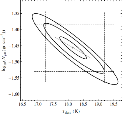
Figure 3: Contour map of $\Delta\chi^{2}=\chi^{2}-\chi^{2}_{\rm min}$ for an arbitrary pixel around $\Delta\chi^{2}=0$. Contour levels are 0.45, 2.3, and 4.61, corresponding to 0.25, 1.0, and 1.6 $\sigma$, respectively. Dashed lines display the predictions of Equations (9) which approximate the 1-$\sigma$ contour projection onto the axes. The thin gray line that crosses the best fit point has the direction of the curve $N_{g}T_{d}=\text{constant}$.

Equations (9) and (10) were derived by fitting the upper and lower limits of $T_{d}$ and $\log N_{g}$ projections of the uncertainty region. These approximations for the uncertainty are valid for $T_{d}$ between 7 and 40 K, for $\log N_{g}$ between $-3.4$ and $1.1$ (equivalent to $\log N_{\rm H_{2}}$ between 19.9 and 24.4), and for values of $\eta_{10}$ between 1 and 2, which correspond to 10% and 20% calibration errors, respectively. Figure 3 shows an example of the prediction of Equations (9) compared to the $\Delta\chi^{2}$ contours. Within their range of validity and for data taken in the nominal mode, the intervals $\left[T_{d}-\delta T^{-},T_{d}+\delta T^{+}\right]$ and $\left[\log N_{g}-\delta\log N_{g},\log N_{g}+\delta\log N_{g}\right]$ correspond to the projections of the uncertainty ellipse onto the $T_{d}$ and $\log N_{g}$ axes within 0.2 K and 0.02 dex, respectively.

Equations (9) also indicate that, while the confidence interval of $\log N_{p}$ is symmetric and roughly constant, the temperature uncertainties grow rapidly above 25 K and they are skewed towards the higher value (Hoq et al., 2013). This is produced mainly because of the absence of data at wavelengths shorter than 160 $\mu$m. As explained in Section 3.3, we do not use the 70 µm data in our model. Including the 70 $\mu$m data increases the median of the $\chi^{2}_{r}$ distribution to $\sim 3.5$. The temperature and log-column density uncertainties are also correlated along the approximate direction where the product $T_{d}\times N_{g}$ is constant, indicated in Figure 3. The better the R-J approximation is for the SED, the better will be the alignment of the major axis of the ellipse with the line $T_{d}\times N_{g}=\text{constant}$.

3.5 Saturated Sources

The HSO detectors in SPIRE and PACS have saturation limits that depend on the observing mode. The saturation intensities for the nominal observing mode are 220 and 1125 Jy beam^-1 for the 70 and 160 $\mu$m PACS bands, respectively, and 200 Jy beam^-1 for SPIRE. Saturation is most problematic in the 250 $\mu$m SPIRE band.

There are 46 MALT90 sources whose Hi-GAL data are affected by saturation. Of these, six are covered by HOBYS observations made by using the bright mode (Section 2.2) that gives reliable 250 $\mu$m intensities. For the remaining 40 sources, we replace the saturated pixels with the saturation limits given above, and we fit the SED taking these values as lower bounds.

3.6 The 70 $\mu$m Appearance of the Quiescent Clumps

MALT90 and other previous studies (e.g., Molinari et al., 2008; López-Sepulcre et al., 2010; Sanhueza et al., 2012; Sánchez-Monge et al., 2013; Giannetti et al., 2013; Csengeri et al., 2014) use mid-IR observations as a probe of star formation activity. However, deeply embedded, early star formation activity could be undetected at mid-IR yet be conspicuous at far-IR. Quantitatively, we expect that the 24 to 70 $\mu$m flux density ratio of HMYSOs to vary between $10^{-6}$ and 1 for a wide range of molecular core masses (60 to 240  $M_{\odot}$) and central star masses over 1  $M_{\odot}$ (Zhang et al., 2014). Therefore, despite MIPSGAL having $\sim 50$ times better point source sensitivity at 24 µm than that of Hi-GAL at 70 µm, it is possible to detect embedded protostars in 70 $\mu$m images that would otherwise appear dark at 24 $\mu$m and would be classified as Quiescent. The 70 $\mu$m data thus allow us to further refine the MALT90 classification since a truly Quiescent clump should lack 70 $\mu$m compact sources (e.g., Sanhueza et al., 2013; Beuther et al., 2013; Tan et al., 2013).

We examined the Hi-GAL 70 $\mu$m images of the 616 Quiescent sources and found 91 (15%) that show compact emission at 70 $\mu$m within 38″ – or one Mopra telescope beamsize – of the nominal MALT90 source position. Hereafter, we consider these sources as part of the Protostellar sub-sample. We also found 83 sources that appear in absorption at 70 $\mu$m against the diffuse Galactic emission. We refer to these clumps as far-IR dark clumps (far-IRDCs). The remaining 442 Quiescent sources are either associated with diffuse emission not useful for tracing embedded star formation, or they are confused with the 70 $\mu$m diffuse emission from the Galactic plane.

4 DISCUSSION

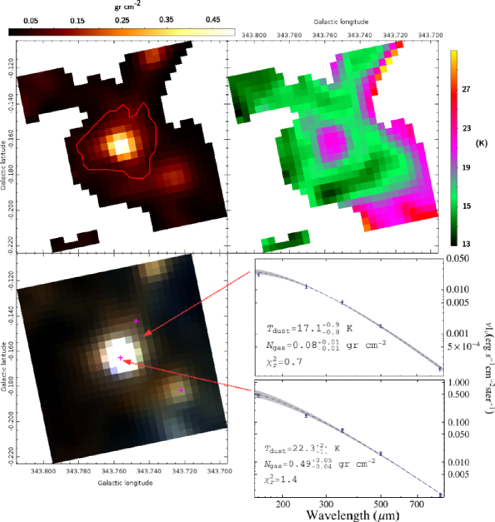
Figure 4: Parameters and data around AGAL343.756$-$00.164. Bottom panels show a three color image (500, 250, and 160 $\mu$m for red, green, and blue, respectively) centered on AGAL343.756$-$00.164 and two SED fittings performed over the intensities measured toward two positions, marked by red arrows: one located toward the center of the MALT90 source and the other toward its periphery. The three crosses mark the position of adjacent MALT90 sources. The top-left panel shows the best-fit column density map. The red contour marks the area that defines the AGAL343.756$-$00.164 clump. Blanked pixels do not have intensities larger than $2\sigma$ in at least one of the bands (see Section 3.3). The top-right panel shows the best-fit dust temperature map.

Figure 4 shows the dust temperature and column density obtained for each pixel around the source AGAL343.756$-$00.164, which is taken as a typical example. Best-fit dust temperatures, column densities, and their uncertainties are calculated pixel by pixel. The two plots located in the lower-right corner of Figure 4 show the SED measured in two directions (center and periphery) toward AGAL343.756$-$00.164. The blue dashed line in each of these plots is the curve given by Equation (1) evaluated in the best fit solution. The shaded region around the curve is the locus covered by the model when the best-fit parameters vary within the 1-$\sigma$ confidence interval. As explained in Section 3.3, the $\chi^{2}$ is calculated by comparing the measured intensities at each band with the SED model weighted by the respective bandpasses.

Table 3 gives the derived dust temperatures and log-column densities of 3218 MALT90 sources. This correspond to a 99.1% of the 3246 ATLASGAL sources observed by MALT90. The remaining 28 sources are either not covered by HSO observations (24 sources) or they are too faint to reliably estimate the dust parameters (4 sources). Column 1 indicates the ATLASGAL name of the source. We include 311 entries which correspond to multiple sources blended along the same line of sight, indicated with an “m” superscript. Column 2 gives the effective angular radius of the source in arcsec, defined as $\theta_{\rm eff}=\sqrt{\Omega_{s}/\pi}$, where $\Omega_{s}$ is the effective angular area occupied by the MALT90 source. This area corresponds to the intersection between the region enclosing the source where the column density is greater than 0.01 gr cm^-2 ($>2.0\times 10^{21}$ cm^-2 in H₂ column density) and the 870 $\mu$m ATLASGAL mask (see Contreras et al., 2013 and Urquhart et al., 2014b). Figure 4 shows an example of one of these areas (red contour in top left image). Column 3 of Table 3 gives the mean dust temperature averaged over the area of each source ($\bar{{T_{d}}}$). Columns 4 and 5 list the lower and upper uncertainty of $\bar{T_{d}}$, respectively. Columns 6, 7, and 8 give the dust temperature at the position of the 870 $\mu$m peak intensity ($T_{d,{\rm P}}$) and its lower and upper uncertainties, respectively. Columns 9, 10, and 11 list the average column density ($\bar{N_{g}}$), its logarithm, and the uncertainty of the latter, respectively. Columns 12 gives the peak column density ($N_{g,{\rm P}}$), derived using the 870 $\mu$m peak intensity and $T_{d,{\rm P}}$ (in Equations (1), (2) and (3)). Columns 13 and 14 give $\log N_{g,{\rm P}}$ and its uncertainty, respectively. Finally, column 15 gives the mid-IR classification of the MALT90 source, as Quiescent (616 clumps), Protostellar (749 clumps), Hii region (844 clumps), PDR (343 clumps), or Uncertain (666 clumps). Note that these numbers describe the statistics of Table 3, that is, of the 3218 sources for which we have dust column density and temperature estimations. For the Quiescent sources, we indicate with a superscript “C” or “D” whether the source is associated with 70 $\mu$m compact emission or if it is a far-IRDC, respectively (see Section 3.6). No superscript means that neither of these features appears related to the clump.

Previous studies of massive molecular clumps have relied on samples obtained from the IRAS catalog and fit SEDs to obtain dust temperatures and masses. We find a total of 116 matches between MALT90 and those samples as analyzed by Faúndez et al. (2004, 94 matching sources) and Giannetti et al. (2013, 22 matches). Other studies, such as Sridharan et al. (2002) and Williams et al. (2005), have targeted the northern sky and they do not overlap significantly with MALT90 (1 source in common each). From all these sources, 63 are classified as Hii region, 44 as Protostellar, 3 as PDR, 6 as Quiescent, and 2 as Uncertain. From the relative fraction of Quiescent sources in the MALT90 sample, we would expect 13 or more of the 118 to be Quiescent with a 99% probability, assuming that they are randomly sampled. Since there are only 6 Quiescent matches, we conclude that previous surveys were biased toward more evolved stages, illustrating how MALT90 helps to fill in the gap in the study of cold clumps.

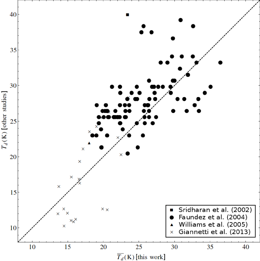
Figure 5: Comparison between the dust temperatures obtained in the present work and the dust temperatures obtained from Sridharan et al. (2002), Faúndez et al. (2004), Williams et al. (2005), and Giannetti et al. (2013). The dust temperatures of Faúndez et al. (2004) and Giannetti et al. (2013) have been re-scaled according to the assumed value of $\beta$ using Equation (7). The dashed line shows the identity line.

Figure 5 shows the dust temperature calculated by previous studies versus the dust temperatures given in this work. We calculate a Spearman correlation coefficient (Wall & Jenkins, 2012, Section 4.2.3) of 0.75 with a 95% confidence interval between 0.68 and 0.83, indicating a positive correlation between our temperature estimations and those from the literature. Faúndez et al. (2004) assume a dust absorption spectral index $\beta=1$, while our dust model is characterized by $\beta\approx 1.7$. Therefore, we correct their temperatures according to Equation (7) by multiplying them by $(3+1)/(3+1.7)\approx 0.85$. The correction decreases the mean of the differences between the dust temperatures obtained by Faúndez et al. (2004) and the temperatures obtained by us from $+7$ K (uncorrected) to $+2$ K. We apply the same correction to the temperatures given by Giannetti et al. (2013) using their reported best-fit $\beta$ values. Figure 5 shows that temperatures estimated using data from mid- and far-IR bands below 100 $\mu$m are more often higher than the dust temperatures derived in this work. In consequence, the slope of a linear regression performed in the data shown in Figure 5 is slightly larger than unity ($1.13\pm 0.09$). This is somewhat expected since our own single temperature SED model underestimates the 70 $\mu$m intensity (see Section 3.3). The most plausible reason is that in these sources there is a warmer dust component better traced by IR data below 100 $\mu$m.

Dust temperatures and column densities of a preliminary MALT90 subsample consisting of 323 sources were presented by Hoq et al. (2013). They also use the Hi-GAL data (without ATLASGAL) and they employ a similar data processing and SED fitting procedure compared to that used in this work. Hoq et al. (2013) report dust temperatures which are consistent within 13% compared to the ones given in Table 3. However, we obtain average column densities that are smaller by about 20%. The differences are due to our source sizes being larger than the ones assumed by Hoq et al. (2013). They use a fixed size equal to one Mopra telescope beam, while we define the size of the source based on its extension in the column density map.

When there is more than one source in the same line of sight, the continuum emission blends two or more clumps located at different distances. This makes uncertain the interpretation of the temperature, column density, and evolutionary stage classification. Therefore, for further analysis we remove these sources from the MALT90 sample, leaving 2907 sources. This number breaks down in the following way (see Table 4): there are 464 sources considered as Quiescent (single V_LSR, without a compact 70 $\mu$m source), 788 considered Protostellar (including Quiescents with a 70 $\mu$m compact source), 767 Hii regions, and 326 PDRs. The remaining sources (562) have an Uncertain classification. This selection and reclassification of sources, as we show in Appendix A, does not affect the conclusions presented in the following sections.

4.1 Dust Temperature versus Gas Temperature

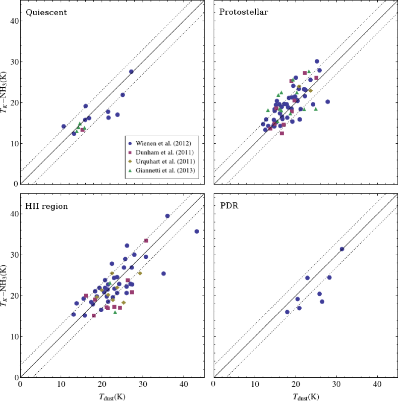
Figure 6: From left to right and top to bottom: dust temperature versus kinetic ammonia temperature of 15 Quiescent, 69 Protostellar, 58 Hii region, and 8 PDR MALT90 sources. Ammonia temperatures were obtained from Wienen et al. (2012), Dunham et al. (2011), Urquhart et al. (2011), and Giannetti et al. (2013). The continuous and both dotted lines in each panel display the identity and the identity $\pm 3$ K relations, respectively.

The dust temperature is fixed by the balance between heating and radiative cooling of the grain population. If the density in a molecular cloud is greater than $5\times 10^{4}$ cm^-3 (Goldsmith, 2001; Galli et al., 2002), we expect the dust temperature to be coupled to the gas temperature. We test this hypothesis by comparing the average dust temperatures with the gas kinetic temperatures determined from ammonia observations. Figure 6 shows the ammonia temperature derived by Dunham et al. (2011, 23 matching sources), Urquhart et al. (2011, 10 matching sources), Wienen et al. (2012, 106 matching sources), and Giannetti et al. (2013, 19 sources) versus the dust temperature, separated by evolutionary stage. Dunham et al. (2011) and Urquhart et al. (2011) performed the NH₃ observations using the Green Bank Telescope at 33″ angular resolution. Wienen et al. (2012) used the Effelsberg Radiotelescope at 40″ angular resolution. These are comparable to the resolution of our dust temperature maps (35″). On the other hand, Giannetti et al. (2013) used NH₃ data obtained from ATCA with an angular resolution of $\sim 20\arcsec$. In this last case, we compare their ammonia temperatures with $T_{d,{\rm P}}$ instead of $\bar{T_{d}}$.

All but eight MALT90 sources with ammonia temperature estimation are classified in one of the four evolutionary stages. The Spearman correlation coefficient of the entire sample (158 sources, including these eight with Uncertain mid-IR classification) is 0.7, with a 95% confidence interval between 0.6 and 0.8, indicating a positive correlation between both temperature estimators. The scatter of the relation is larger than the typical temperature uncertainty, and it grows with the temperature of the source. For sources below 22 K, ammonia and dust temperatures agree within $\pm 3$ K. Above 22 K, the uncertainties of both temperature estimators become larger (see Equations (9) and, for example, Walmsley & Ungerechts, 1983), consistent with the observed increase of the scattering. In addition, higher temperature clumps are likely being heated from inside and therefore associated with more variations in the dust temperatures along the line of sight, making the single temperature approximation less reliable. The slopes of the linear regressions performed in the data are $0.7\pm 0.1$, $0.8\pm 0.1$, $0.7\pm 0.1$, and $0.9\pm 0.3$ for the Quiescent, Protostellar, Hii region, and PDR samples, respectively. The ammonia and dust temperatures relation agrees in general with that found by Battersby et al. (2014), except that we do not find a systematically worse agreement on Quiescent sources compared with the other evolutionary stages.

4.2 Temperature and Column Density Statistics

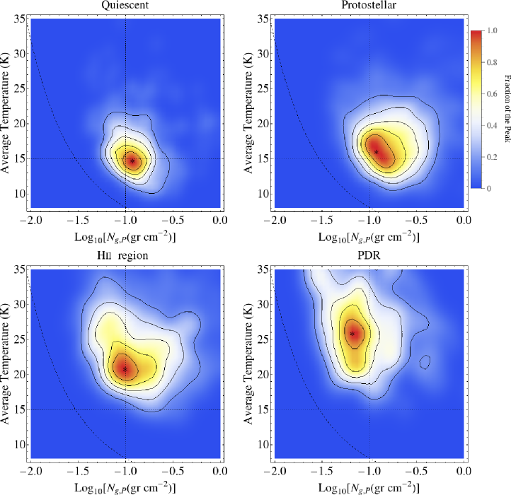
Figure 7: Color map of smoothed 2-D histograms of the distributions of temperature and log peak column density for each evolutionary stage. The smoothing was implemented using a Gaussian kernel with a standard deviation of 25% of the observed dispersion in each direction. The color scale indicates the fraction of the peak according to the colorbar. Five contours are taken from one to five sixths of the peak. An asterisk shows the position of the peak of each distribution. The dashed line indicates the 0.5 Jy level at 870 $\mu$m (assuming the dust model described in Section 3.3), which is roughly the completeness limit of MALT90 (Jackson et al., 2013). The two dotted lines drawn at $\log(N_{g,{\rm P}})=-1.0$ and $\bar{T_{d}}=15$ K are fiducial values used to facilitate the comparison among the different panels.

Figure 7 shows maps of smoothed 2-D histograms of the distributions of $\bar{T_{d}}$ and $\log N_{g,{\rm P}}$ of the MALT90 clumps for each mid-IR classification. In the following analysis we focus on these two quantities and their relation with the evolutionary stage. We use $N_{g,{\rm P}}$ instead of $\bar{N_{g}}$ because $N_{g,{\rm P}}$ is independent of the specific criterion used to define the extension of the clump and because the column density profiles are often steep ($\propto s^{-0.8}$, where $s$ is the plane-of-the-sky distance to the clump center, Garay et al., 2007), making the average $\bar{N_{g}}$ less representative of the clump column density values. On the other hand, dust temperature gradients are shallower ($\propto r^{-0.4}$, where $r$ is the distance to the clump center, see van der Tak et al., 2000) and $\bar{T_{d}}$ has less uncertainty compared with the temperature calculated toward a single point. We include in the Protostellar group those sources that are associated with a compact source at 70 $\mu$m (Section 3.6). The most conspicuous differences between the evolutionary stages are evident between the Quiescent/Protostellar and the Hii region/PDR populations (Hoq et al., 2013). The main difference between these groups is the temperature distribution. Most of the sources in the Quiescent/Protostellar stage have temperatures below 19 K, while most Hii region/PDR sources have temperatures above 19 K. We also note that the Quiescent, Protostellar, and Hii region populations have peak column densities $\gtrsim 0.1$ gr cm^-2, equivalent to $2.13\times 10^{22}$ H₂ molecules per cm², while the PDR population has peak column densities of typically half of this value.

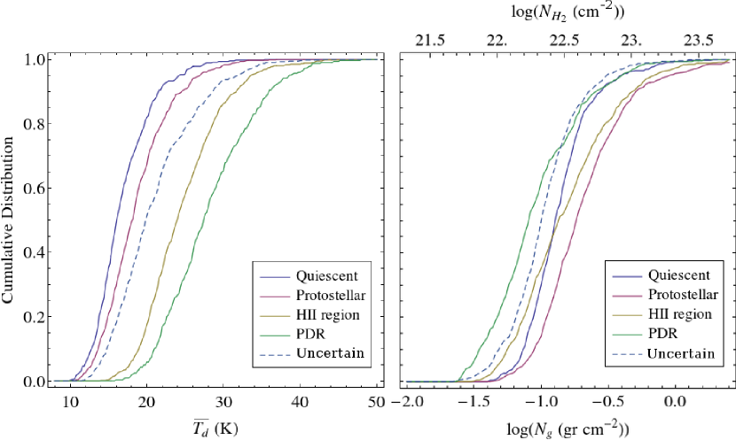
Figure 8: The empirical cumulative distribution functions of $\bar{T_{d}}$ (left panel) and $\log N_{g,{\rm P}}$ (right panel) for each evolutionary stage (continuous lines) and the Uncertain group (dashed lines). The upper axis labeling of the right panel shows the equivalent logarithm of the H₂ column density ($\log N_{\rm H_{2}}$).

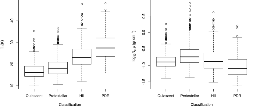
Figure 9: Box-plots of the marginalized temperature and log-peak column density distributions. The thick line indicates the median, the boxes enclose the interquartile range (50% of the total population), and the error bars indicate the minimum and maximum data points that are within $1.5$ times the inter-quartile distance from the boxes’ limits. The remaining points are individually marked with circles as outliers.

These differences are also apparent in Figure 8, where solid lines display the marginalized CDFs of $\bar{T_{d}}$ and $\log N_{g,{\rm P}}$ for each evolutionary stage. The dashed lines show the distributions of the Uncertain group. It is clear from these plots that the median temperature increases monotonically with evolutionary stage, and that the Protostellar and PDR clumps are the stages associated with the largest and smallest column densities, respectively. Figure 9 shows Tukey box plots (Feigelson & Babu, 2012, Section 5.9) of the marginalized distributions of $\bar{T_{d}}$ and $\log N_{g,{\rm P}}$ separated by evolutionary stage. In these plots, the boxes indicate the interquartile range (half of the population), the thick horizontal line inside each box indicates the median, and the error bars encompass the data that are within 1.5 times the inter-quartile distance from the box limits. The remaining points, in all cases less than 4% of the sample, are plotted individually with small circles and we refer to them formally as outliers. Figure 9 shows that the $\bar{T_{d}}$ and $\log N_{g,{\rm P}}$ interquartile range shifts with evolutionary stage. This is evidence of systematic differences between the different populations, despite the large overlaps. In practice, the overlap between populations implies that it is unfeasible to construct sensible predictive criteria that could determine the evolutionary stage of a specific source based on its temperature and peak column density and it also reflects that star formation is a continuous process that cannot be precisely separated into distinct stages. Nevertheless, the fact that the proposed evolutionary stages show a monotonic increase in mean temperature demonstrates that the classification scheme has a legitimate physical basis.

In the following, we focus our analysis on the Quiescent and Protostellar populations. Figures 7 to 9 show that these two samples are similarly distributed and they exhibit the most important overlap. We test the statistical significance of the Quiescent and Protostellar differences in $\bar{T_{d}}$ and $\log N_{g,{\rm P}}$ by comparing these differences with their uncertainties. Table 4 shows the medians, means, and r.m.s. deviations of $\bar{T_{d}}$, $T_{d,{\rm P}}$, $\log\bar{N_{g}}$, and $\log N_{g,{\rm P}}$ for each population. In general, these dispersions are larger than the uncertainties of the individual values, indicating that the dispersions are intrinsic to each population and not due to the fitting uncertainties. The means $\bar{T_{d}}$ for the Quiescent and Protostellar populations are $16.8$ and $18.6$ K, respectively. The Protostellar population has a mean $\bar{T_{d}}$ larger by $+1.8$ K compared with the Quiescent population. We can estimate the expected uncertainty of this mean difference using the dispersion and size of each population, which gives $\sqrt{\left(3.8^{2}/464\right)+\left(4.4^{2}/788\right)}\approx 0.24$ K. Therefore, the difference is more than seven times the expected uncertainty. On the other hand, the difference of the means of $\log N_{g,{\rm P}}$ is $+0.17$ in favor of the Protostellar population. The expected uncertainty in this case is $\sqrt{\left(0.25^{2}/464\right)+\left(0.34^{2}/788\right)}=0.017$, that is, ten times smaller than the observed difference. We conclude that the observed differences of the Quiescent and Protostellar populations are statistically significant. Furthermore, the differences in temperature and column density are orthogonal to the expected uncertainty correlation (Figure 3), giving us more confidence that we are observing a real effect in both parameters. We confirm the significance of the difference using more sophisticated statistical tests in Appendix A. Note that either the temperature or the column density difference between other population pairs are larger than those between the Quiescent and Protostellar.

Are these statistical differences evident when comparing the $\bar{N_{g}}$ and $T_{d,{\rm P}}$? On one hand, the difference between the mean $T_{d,{\rm P}}$ of the Protostellar and Quiescent samples is 2.6 K, while the expected uncertainty of this difference is 0.2 K. Therefore, despite the larger fitting uncertainties of $T_{d,{\rm P}}$ (see Table 3), we still detect a statistically significant difference between both populations when comparing only their central temperatures. On the other hand, the difference between the means of $\log\bar{N_{g}}$ is $0.04$ over an expected uncertainty of $0.02$, that is, the difference is only 2 times the uncertainty. The latter is not highly significant, which is somehow expected because of the reasons explained at the beginning of this section. It is also expected from previous studies that indicate that neither the mass of the clumps (Hoq et al., 2013) nor their radii (Urquhart et al., 2014b) change conspicuously with evolutionary stage. This in turn implies that the average column density should remain approximately unchanged.

Within the Quiescent sample, we identified in Section 3.6 a population of 83 clumps that appear as far-IRDCs at 70 $\mu$m. Of these, there are 77 associated with a single source along the line of sight. This sample has a mean and median $\bar{T_{d}}$ of $14.9$ and $14.7$ K, respectively. The remaining Quiescent population has mean and median $\bar{T_{d}}$ equal to $17.2$ and $16.4$ K, respectively. Based on a Wilcoxon non-parametric test (Wall & Jenkins, 2012, Section 5.4) we obtain a p-value of $4\times 10^{-7}$ under the null hypothesis that these distributions are the same. Therefore, the temperature differences between the far-IRDCs and the rest of the Quiescent clumps are significant. The column densities of the far-IRDC subsample are also larger compared to those of the rest of the Quiescent sample. The far-IRDC $\log N_{g,{\rm P}}$ mean and median are $-0.76$ and $-0.78$, respectively, while for the remaining Quiescent clumps they are $-0.88$ and $-0.91$, respectively. Again, we reject the null hypothesis (Wilcoxon p-value of $\sim 10^{-5}$) and conclude that the far-IRDC sample is a colder and denser subsample of the Quiescent population.

Finally, the Uncertain group (that is, MALT90 sources that could not be classified into any evolutionary stage) seems to be a mixture of sources in the four evolutionary classes, but associated with lower column densities (median $\log N_{g,{\rm P}}\sim 0.1$ gr cm^-2). Figure 8 shows that the $\bar{T_{d}}$ values of the Uncertain group distribute almost exactly in between the other evolutionary stages. Neither a Wilcoxon nor a Kolmogorov-Smirnov test can distinguish the $\bar{T_{d}}$ distributions of the Uncertain sample from the remainder of the MALT90 sources combined with a significance better than 5%. Figure 8 also shows that the column densities of the Uncertain group are in general lower compared with those of any evolutionary stage except the PDRs. Molecular clumps with low peak column density may be more difficult to classify in the mid-IR, since they are probably unrelated to high-mass star formation. It is also possible that a significant fraction of these sources are located behind the Galactic plane cirrus emission and possibly on the far-side of the distance ambiguity, making the mid-IR classification more difficult and decreasing the observed peak column density because of beam dilution.

4.2.1 Column Density and Temperature Evolution in Previous Studies

Since the discovery of IRDCs (typically dark at mid-IR wavelengths, see Egan et al., 1998; Carey et al., 1998) it has been pointed out that they likely consist of cold ($<20$ K) molecular gas. This has been confirmed by several studies of molecular gas (Pillai et al., 2006; Sakai et al., 2008; Chira et al., 2013) and dust (e.g., Rathborne et al., 2010).

Systematic H₂ column density differences between IR dark, quiescent, and star-forming clumps have been more difficult to establish. Some authors have found no significant column density differences between these groups (Rathborne et al., 2010; López-Sepulcre et al., 2010; Sánchez-Monge et al., 2013). However, most studies based on large samples agree that star forming clumps have larger molecular column densities compared to the quiescent ones (Dunham et al., 2011; Giannetti et al., 2013; Hoq et al., 2013; Csengeri et al., 2014; Urquhart et al., 2014b; He et al., 2015). Furthermore, Beuther et al. (2002), Williams et al. (2005), and Urquhart et al. (2014b) found evidence that molecular clumps which display star formation activity have a more concentrated density profile.

Urquhart et al. (2014b), based on ATLASGAL and the Red MSX Source (RMS) survey (Lumsden et al., 2013), analyze a large ($\sim 1300$) number of molecular clumps with signs of high-mass star formation. High-mass star formation activity was determined from associations with the MSX point source catalog (Egan et al., 2003), methanol masers (Urquhart et al., 2013a), and Hii regions detected using centimeter wavelength radio emission (Urquhart et al., 2007, 2009, 2013b). In Urquhart et al. (2014b), ATLASGAL clumps associated with WISE sources (Wright et al., 2010) are called massive star-forming (MSF) clumps and all the rest are otherwise “quiescent.” Urquhart et al. (2014b) find that MSF clumps have larger column densities than their “quiescent” clumps by a factor of $\sim 3$.

Urquhart et al. (2014b) and He et al. (2015) also report that clumps associated with Hii regions have larger column densities than the remainder of the star forming clumps. This result contradicts our finding that Hii region sources have typically lower column densities compared with the Protostellar sample (see Table 4 and Figure 8). To examine this disagreement in more detail, we analyze the intersection between the MSF and the MALT90 samples. There are 515 MSF clumps in common with the MALT90 sample that are covered by Hi-GAL: 285 classified as Hii regions, 204 as Protostellar, 22 as PDR, and 4 as Quiescent. We calculate that these 515 sources have a mean average temperature of 24 K and a mean log-peak column density of $-0.63$. The temperature is consistent with the Hii region sample of MALT90, but the column densities are much higher. Within these 515 sources we find that, in agreement with Urquhart et al. (2014b), those with centimeter wavelength emission have significantly higher column densities ($\log N_{g,{\rm P}}=-0.59$) and temperatures ($26$ K) compared with the rest ($\log N_{g,{\rm P}}=-0.67$ and $\bar{T_{d}}=22$ K).

The reason for Urquhart et al. (2014b) finding that sources associated with Hii regions are associated with the largest column densities, in disagreement with our results, arises most likely from differences in the classification criteria. Urquhart et al. (2014b) report centimeter radio emission arising from ionized gas toward 45 out of the 204 common sources we classify as Protostellar, and 94 out of the 285 clumps we classify as Hii regions were observed by the CORNISH survey at 5 GHz ($\sim 2$ mJy sensitivity, Hoare et al., 2012) and were not detected. These are relatively few sources and exchanging their classification (Protostellar by Hii region and vice-versa) does not modify the trends described in the previous section. However, if they reflect an underlying fraction of misclassified sources between the Protostellar and Hii region groups, they might change the statistics.

Conversely, we detect embedded HMYSOs in 641 ATLASGAL sources that are treated as “quiescent” in Urquhart et al. (2014b), in part due to the better sensitivity and angular resolution of MIPS compared to MSX and WISE. It is likely that the “quiescent” sample of Urquhart et al. (2014b) does not contain currently young high-mass stars, but does contain a large fraction of intermediate mass star formation activity, and some of these sources are also associated with PDRs. In summary, we expect that the Quiescent sample from MALT90 to be more truly devoid of star formation than the non-MSF ATLASGAL clumps, while at the same time, several of our Protostellar clumps are probably associated with Hii regions, which are more efficiently detected using radio centimeter observations.

4.2.2 Temperature and Column Density Contrasts

We analyze spatial variations of $T_{d}$ and $N_{g}$ by comparing their values at the peak intensity position with the average value in the clump. For each MALT90 clump, we define the temperature contrast and log-column density contrast as $\Delta T=\bar{T_{d}}-T_{d,{\rm P}}$ and $\Delta\log N_{g}=\log\left(\bar{N_{g}}/N_{g,{\rm P}}\right)$, respectively.

Table 5 lists the means and medians of the temperature and log-column density contrasts. Table 5 also gives 95% confidence intervals (CIs) for the medians of $\Delta T$ and $\Delta\log N_{g}$ per evolutionary stage, determined using the sign test (Ross, 2004, Section 12.2). They were calculated using the task SIGN.test from the R statistical suite (version 3.1.1). The sign test is not very sensitive but it has the advantage that it is non-parametric and, in contrast to the Wilcoxon test (for example), it does not assume that the distributions have the same shape.

A negative $\Delta\log N_{g}$ indicates that the clump has a centrally peaked column density profile with the absolute value of $\Delta\log N_{g}$ being a measure of its steepness. As a reference, a critical Bonnor-Ebert sphere is characterized by $\Delta\log N_{g}=-0.5515$. Perhaps not very surprisingly, the $\Delta\log N_{g}$ means, medians, and CIs are always negative, indicating that most of the clumps are centrally peaked. We find that the medians are significatively different between evolutionary stages, with no overlap in the CIs. The Hii region clumps are those associated with the steepest column density profiles, followed by the Protostellar and the PDR clumps. Clumps in the Quiescent evolutionary stage are associated with the smoothest column density profiles.

The temperature contrasts are also distinct for different evolutionary stages. A positive $\Delta T$ indicates that the dust temperature increases away from the clump center, that is, dust temperature at the peak column density position ($T_{d,{\rm P}}$) being lower than the average temperature ($\bar{T_{d}}$). On the other hand, $\Delta T$ is negative for decreasing temperature profiles. $\Delta T$ is positive for Quiescent clumps and PDRs, it is consistent with zero for the Protostellar sources (temperature at peak similar to average temperature), and positive (peak column density warmer than average temperature) for the Hii region sample.

4.3 Mid-IR Classification versus $T_{d}$, $N_{g}$, $\Delta T_{d}$, and $\Delta\log N_{g}$

The previous sections have presented the differences between the temperature and column densities of the MALT90 groups. These differences are qualitatively consistent with the evolutionary sequence sketched in Jackson et al. (2013) that starts with the Quiescent, and proceeds through the Protostellar, Hii region, and PDR evolutionary stages. As Figure 9 shows, Quiescent clumps are the coldest, in agreement with the expectation that these clumps are starless and there are no embedded young high-mass stars. The far-IRDC subsample of the Quiescent population is colder and denser on average compared to the rest of the Quiescent clumps, and they might represent a late pre-stellar phase just before the onset of star-formation. The mean temperature and $\log N_{g,{\rm P}}$ of the far-IRDC subsample are $\sim 15$ K and $-0.78$, respectively.

To establish what fraction of the Quiescent clumps might evolve to form high-mass stars, we use for now criteria defined by previous authors based on distance independent information, such as the column density; a more complete analysis will be done in Contreras et al. (in preparation). Lada et al. (2010) and Heiderman et al. (2010) propose that the star formation rate in a molecular cloud is proportional to the mass of gas with column densities in excess of $\sim$120  $M_{\odot}$ pc^-2 ($\sim 2.43\times 10^{-2}$ gr cm^-2). Since there is considerable overlap in column density between MALT90 clumps that have different levels of star formation activity, we start by assuming that this relation gives the average star formation rate over the timescale of 2 Myr adopted by Lada et al. (2010) and Heiderman et al. (2010). We find that 98% of the Quiescent clumps have $\bar{N_{g}}>120$  $M_{\odot}$ pc^-2, including all of the far-IRDCs, which suggest that most of these clumps will support some level of star formation activity in the future. Urquhart et al. (2014b) propose a column density threshold of $0.05$ gr cm^-2 for what they denominate “effective” high-mass star formation. This same threshold was recently proposed by He et al. (2015) based on a study of $405$ ATLASGAL sources. Of the Quiescent sample, 78% of the clumps have an average column density above this threshold, with the percentage increasing to 92% for the far-IRDCs. Based on these criteria, we conclude that virtually all Quiescent clumps will develop at least low-mass star formation activity and that a large fraction ($>70\%$) will form high-mass stars. On the other hand, López-Sepulcre et al. (2010) suggest a third column density threshold based on the observed increase of molecular outflows for clumps with column densities in excess of $0.3$ gr cm^-2. This column density is significatively larger than the previous thresholds, and only 3% and 6% of the Quiescent and far-IRDCs populations, respectively, have larger average column densities. However, half of the clump sample of López-Sepulcre et al. (2010) have diameters $<35\arcsec$ (the beam size of our column density maps) and more than a third have masses $<200\mbox{\,$M_{\odot}$}$, which indicates that the $0.3$ gr cm^-2 threshold may be pertinent for more compact structures than the clumps considered in this work.

The temperature and temperature contrast of the Quiescent clumps are qualitatively consistent with equilibrium between the interstellar radiation field and dust and gas cooling (Bergin & Tafalla, 2007). We find that Quiescent clumps are the coldest among the evolutionary stages, but they are typically warmer ($\sim 17$ K) than expected from thermal equilibrium between dust cooling and cosmic ray heating alone ($T_{d}\sim 10$ K). We also find that the central regions of the Quiescent clumps are in general colder than their external layers ($\Delta T$ negative). These characteristics are consistent with Quiescent clumps being heated by a combination of external radiation and cosmic-rays. The Quiescent sources also have the flattest density structure, with the largest $\Delta\log N_{g}$ among all the other evolutionary stages. This is similar to the behavior found by Beuther et al. (2002), that is, the earliest stages of high-mass star formation are characterized by flat density profiles that become steeper as they collapse and star formation ensues.

The Protostellar clump sample can be distinguished from Quiescent clumps based on their column density and dust temperature. Protostellar clumps have larger column densities ($\sim 0.2$ gr cm^-2) and are slightly warmer ($\sim 19$ K). The central temperatures of the Protostellar clumps also increase and become comparable to the temperature in their outer regions ($\Delta T\cong 0$). These characteristics indicate that Protostellar clumps have an internal energy source provided by the HMYSOs. According to the results presented by Hoq et al. (2013), there is no significative difference in the distribution of masses between the Quiescent and Protostellar population. If we assume that this is also the case for the sample presented in this work (which will be confirmed in upcoming publications, see also He et al., 2015), then the most likely reason for the larger column densities of the Protostellar sample compared with the Quiescent sample is gravitational contraction. Because contraction develops faster on the densest, central regions, we expect the column density profiles to become steeper at the center of the clump. This is consistent with the observed decrease of $\Delta\log N_{g}$ for the Protostellar clumps compared with the Quiescent clumps.

The Hii region sample is associated with the most negative temperature and column density contrasts (median of $\Delta T=-0.33$ K and $\Delta\log N_{g}=-0.42$) compared with any other population, which indicates that Hii region clumps are very concentrated and they have a strong central heating source. This picture is consistent with the presence of a young high-mass star in the center of the clump. The slight decrease of the peak column density compared with the Protostellar phase could be explained because of the expansion induced by the development of the Hii region and the fraction of gas mass that has been locked into newly formed stars.

Finally, PDR clumps have the lowest column densities and largest temperatures among the four evolutionary stages. They are also associated with having colder temperatures toward the center compared to their outer regions. PDR clumps are possibly the remnants of molecular clumps that have already been disrupted by the high-mass stars’ winds, strong UV radiation field, and the expansion of Hii regions. These molecular remnants are being illuminated and heated from the outside by the newly formed stellar population, but probably are neither dense nor massive enough to be able to sustain further high-mass star formation.

5 SUMMARY

We determined dust temperature and column density maps toward 3218 molecular clumps. This number corresponds to more than 99% of the ATLASGAL sources that form the MALT90 sample. We fit greybody models to far-IR images taken at 160, 250, 350, 500, and 870 $\mu$m. This catalog represents the largest sample of high-mass clumps for which both dust temperature and column density have been simultaneously estimated. We summarize the main results and conclusions as follows.

1. The average dust temperature increases monotonically along the proposed evolutionary sequence, with median temperatures ranging from $16.1$ K for the Quiescent clumps to $27.4$ K for the clumps associated with PDRs. This confirms that the MALT90 mid-IR classification broadly captures the physical state of the molecular clumps.

2. The highest column densities are associated with the Protostellar clumps, that is, those that show mid-IR signs of star formation activity preceding the development of an Hii region. The average peak column density of the Protostellar clumps is 0.2 gr cm^-2, which is about 50% higher than the peak column densities of clumps in the other evolutionary stages. We interpret this as evidence of gravitational contraction or possibly that Protostellar clumps are more massive. The latter possibility will be analyzed in future work (Contreras et al., in preparation).

3. The radial temperature gradients within the clumps decrease from positive (higher temperatures in the outer layers of the clump), to null (no dust temperature gradient), and to negative (higher temperatures toward the center of the clump) values associated with the Quiescent, Protostellar, and Hii region clumps, respectively. Quantitatively, the mean difference between the average ($\bar{T_{d}}$) and the central ($T_{d,{\rm P}}$) clump temperatures range between $+0.7$, $-0.1$, and $-0.6$ K for the Quiescent, Protostellar, and Hii region samples, respectively. This confirms that Quiescent clumps are being externally heated and Protostellar and Hii region clumps have an internal embedded energy source.

4. The ratio between the peak and average column density for each clump category ranges between 1.8 and 2.6. The flattest column density profiles are associated with the Quiescent population, becoming steeper for the Protostellar and Hii region clumps. This is qualitatively consistent with the hypothesis of evolution through gravitational contraction, in which the contrast is a measure of evolutionary progress.

5. The PDR clump population is characterized by low column densities ($\sim 0.09$ gr cm^-2), high temperatures ($27$ K), and a positive radial temperature gradient (colder inner regions toward warmer dust on the outside). We interpret this as evidence that these sources are the externally illuminated remnants of molecular clumps already disrupted by high-mass star formation feedback.

6. We identify $83$ far-IR dark clouds, that is, Quiescent clumps that appear in absorption at 70 $\mu$m against the Galactic background. These clumps are cooler and they have higher column densities compared to the remainder of the Quiescent population. Therefore, they are likely in the latest stage of pre-stellar contraction or they may represent a more massive subsample of the Quiescent clumps.

Appendix A Significance Tests on the Difference between the Quiescent and Protostellar Populations

We analyze the statistical significance of the difference between the Quiescent and Protostellar populations using two non-parametric tests: the sign test (Ross, 2004, Section 12.2) and the Kolmogorov-Smirnov (K-S) two sample test (Wall & Jenkins, 2012, Section 5.4). We implement them using the R statistical suite (version 3.1.1) through the tasks SIGN.test and ks.test.

We apply the sign test to evaluate whether the medians of the $\bar{T_{d}}$ and $\log{N_{g,{\rm P}}}$ distributions of the Quiescent and Protostellar samples are significativelly different. Because these two samples are the most similarly distributed, we can conclude that the four evolutionary stages can be distinguish based on their $\bar{T_{d}}$ or $\log{N_{g,{\rm P}}}$ distributions if we can show it for the Quiescent and Protostellar samples.

The median 95% CIs of $\bar{T_{d}}$ and of $\log{N_{g,{\rm P}}}$ are given in Table 6, which shows that the CIs of the Quiescent and Protostellar populations do not overlap. This means that there is no value that is simultaneously consistent (at 5% significance level) with it being the median of the Quiescent and of the Protostellar populations. We call the Original sample (first row of Table 6) that of MALT90 sources analyzed by default throughout this work, that is, the Quiescent and Protostellar sources which are not blended along the same line of sight with another MALT90 source, and with the Quiescent sources associated with compact 70 $\mu$m emission re-classified as Protostellar (see Section 3.6). The second row of Table 6 gives the CIs without applying this re-classification based on the 70 $\mu$m images. The third row shows the CIs associated with the samples from where we have removed the outliers displayed in Figure 9. Finally, the sample of the fourth row takes all MALT90 sources in each category regardless of being multiple sources across the same line of sight. In all cases, we see that the CIs do not overlap. We conclude that the $\bar{T_{d}}$ or $\log{N_{g,{\rm P}}}$ medians are significantly different between the samples and that these differences do not depend critically on the censoring or re-classifications applied in this work.

Table 7 shows the results of the K-S test p-values associated with the null hypothesis that the distributions are the same. We conclude that the probability of the observed data assuming that both samples are drawn from the same distribution is $<10^{-10}$ in all cases. Therefore, we reject the null hypothesis in each case, and conclude that the statistical evidence does not support that the Quiescent and Protostellar samples come from the same underlying distribution. We conclude that the differences between these two evolutionary stages are significant and robust, i.e., they are independent of possibly misclassified sources or outliers.

Table 1: Observational Characteristics of the Data

Instrument	Band	FWHM	$\sigma_{p}$	$\sigma$	Telescope
	($\mu$m)	(″)	(mJy)	(MJy sr-1)
PACS	70	9.2	18	1.1	HSO
PACS	160	12.0	24	1.5	HSO
SPIRE	250	17.0	12	0.7	HSO
SPIRE	350	24.0	12	0.7	HSO
SPIRE	500	35.0	12	0.7	HSO
LABOCA	870	19.2	25	1.5	APEX

Note. — The noise displayed for the SPIRE data is taken in nominal mode. Noise associated with data taken in bright mode is $\sim$4 times higher.

Table 2: HSO Observations

Target	Obs. ID	Obs. Mode	Obs. Date
Field-000_0	1342204102/3	PB	2010-09-07
Field-002_0	1342204104/5	PB	2010-09-07
Field-004_0	1342214761/2	PB	2011-02-24
Field-006_0	1342214763/4	PN	2011-02-24
Field-008_0	1342218963/4	PN	2011-04-09
Field-011_0	1342218965/6	PN	2011-04-09
Field-013_0	1342218999/0	PN	2011-04-10
Field-015_0	1342218997/8	PN	2011-04-10
Field-017_0	1342218995/6	PN	2011-04-10
Field-019_0	1342218644/5	PN	2011-04-15
Field-022_0	1342218642/3	PN	2011-04-15
Field-283_0	1342255009/0	PN	2012-11-14
Field-286_0	1342255011/060	PN	2012-11-14
Field-288_0	1342255061/2	PN	2012-11-15
Field-299_0	1342183075/6	PN	2009-09-03
Field-301_0	1342203083/4	PN	2010-08-15
Field-303_0	1342189081/2	PN	2010-01-08
Field-305_0	1342189083/4	PN	2010-01-08
Field-308_0	1342203085/6	PN	2010-08-16
Field-310_0	1342203278/9	PN	2010-08-20
Field-312_0	1342189109/0	PN	2010-01-09
Field-314_0	1342203280/1	PN	2010-08-21
Field-316_0	1342203282/3	PN	2010-08-21
Field-319_0	1342203289/0	PN	2010-08-21
Field-321_0	1342203291/2	PN	2010-08-21
Field-323_0	1342189878/9	PN	2010-01-29
Field-325_0	1342203293/4	PN	2010-08-22
Field-327_0	1342204042/3	PN	2010-09-03
Field-330_0	1342204044/5	PN	2010-09-04
Field-332_0	1342204046/7	PN	2010-09-04
Field-334_0	1342204054/5	PN	2010-09-04
Field-336_0	1342204056/7	PN	2010-09-05
Field-338_0	1342204058/9	PN	2010-09-05
Field-341_0	1342204094/5	PN	2010-09-06
Field-343_0	1342204092/3	PN	2010-09-06
Field-345_0	1342204090/1	PN	2010-09-06
Field-347_0	1342204100/1	PN	2010-09-06
Field-349_0	1342214510/1	PN	2011-02-20
Field-352_0	1342214575/6	PN	2011-02-20
Field-354_0	1342214713/4	PN	2011-02-24
Field-356_0	1342204368/9	PB	2010-09-12
Field-358_0	1342204366/7	PB	2010-09-12
NGC6334-S	1342239908	SB	2012-03-01
NGC6334-N	1342239909	SB	2012-03-01
M17-S	1342241160	SB	2012-03-04

Table 3: Temperature and Dust Column Density of MALT90 Sources

Source	Effective	Average			Temperature			Average Column			Peak Column			Mid-IR
	Radius	Temperature			at Peak			Density			Density			Classification
	(″)	(K)			(K)			(gr cm-2)			(gr cm-2)
		$\bar{T_{d}}$	$\sigma^{-}$	$\sigma^{+}$	$T_{d,{\rm P}}$	$\sigma^{-}$	$\sigma^{+}$	$\bar{N_{g}}$	$\log\bar{N_{g}}$	$\sigma$	$N_{g,{\rm P}}$	$\log N_{g,{\rm P}}$	$\sigma$
(1)	(2)	(3)	(4)	(5)	(6)	(7)	(8)	(9)	(10)	(11)	(12)	(13)	(14)	(15)
$\cdots$
AGAL000.254$-$00.496	26.2	19.3	0.4	0.4	20.	1.	1.	0.052	$-$1.28	0.02	0.074	$-$1.13	0.04	QuiescentC
AGAL000.259$+$00.017	87.6	20.8	0.1	0.1	19.	1.	1.	0.506	$-$0.296	0.004	0.977	$-$0.01	0.03	Quiescent
AGAL000.264$+$00.032	43.0	20.5	0.3	0.3	19.	1.	1.	0.493	$-$0.307	0.009	0.832	$-$0.08	0.03	Quiescent
AGAL000.268$-$00.084m	44.5	25.2	0.4	0.4	23.	2.	2.	0.056	$-$1.25	0.01	0.115	$-$0.94	0.04	QuiescentD
AGAL000.273$-$00.064m	59.2	26.7	0.3	0.4	25.	2.	2.	0.093	$-$1.031	0.009	0.195	$-$0.71	0.04	Uncertain
AGAL000.274$-$00.501	36.3	25.9	0.5	0.6	27.	3.	3.	0.037	$-$1.43	0.02	0.06	$-$1.22	0.05	PDR
AGAL000.281$-$00.482	58.3	21.2	0.2	0.2	27.	3.	3.	0.093	$-$1.03	0.01	0.186	$-$0.73	0.05	Hii region
$\cdots$

Note. — Parameters and uncertainties are given by $\bar{T_{\!d}}^{\,\sigma^{+}}_{\,\sigma_{-}}$ and $\log(N_{g})\pm\sigma$.

The logarithm of the mass column density is related to the logarithm of the number column density of molecules and H₂ through: $\log N_{g}(\text{gr cm${}^{-2}$})=-23.4146+\log N_{p}(\text{cm${}^{-2}$})=-23.3291+\log N_{\rm H_{2}}(\text{cm${}^{-2}$})$.

Table 4: Average and Dispersion of Dust Temperature and Log-Column Density Distributions

Classification	Number	$\bar{T_{d}}$			$T_{d,{\rm P}}$			$\log\bar{N_{g}}$			$\log N_{g,{\rm P}}$
		Median	Mean	Dev.	Median	Mean	Dev.	Median	Mean	Dev.	Median	Mean	Dev.
		(K)						$\log(\textrm{gr~{}cm}^{-2})$
Quiescent	464	16.1	16.8	3.8	15.6	16.1	3.4	$-1.11$	$-1.11$	0.27	$-0.90$	$-0.86$	0.25
Protostellar	788	18.1	18.6	4.4	18.1	18.7	4.4	$-1.10$	$-1.07$	0.31	$-0.74$	$-0.69$	0.34
Hii region	767	23.0	23.7	5.2	23.6	24.3	5.4	$-1.29$	$-1.24$	0.33	$-0.88$	$-0.82$	0.35
PDR	326	27.4	28.1	5.9	26.4	27.3	5.8	$-1.44$	$-1.40$	0.30	$-1.10$	$-1.04$	0.34
Uncertain	562	19.8	20.9	5.4	19.5	20.2	5.1	$-1.26$	$-1.26$	0.30	$-1.00$	$-0.98$	0.27

Note. — Dev. represents root mean square deviation.

Table 5: Temperature and Log-Column Density Contrasts

Classification	$\Delta T$			$\Delta\log N_{g}$
	Mean	Median	95% CI	Mean	Median	95% CI
Quiescent	+$0.69$	+$0.46$	$[$+$0.39,$+$0.54]$	$-0.24$	$-0.23$	$[-0.24,-0.22]$
Protostellar	$-0.09$	$0.04$	$[-0.03,$+$0.10]$	$-0.38$	$-0.37$	$[-0.39,-0.36]$
Hii region	$-0.58$	$-0.33$	$[-0.43,-0.22]$	$-0.42$	$-0.42$	$[-0.43,-0.40]$
PDR	+$0.79$	+$0.54$	$[$+$0.40,$+$0.75]$	$-0.36$	$-0.34$	$[-0.37,-0.33]$

Note. — $\Delta\log N_{g}=\log\left(\bar{N_{g}}/N_{g,{\rm P}}\right)$ and $\Delta T=\bar{T_{d}}-T_{d,{\rm P}}$ (Section 4.2.2). For values inside the CIs we cannot reject the hypothesis that they are the median with a significance better than 5% using the sign test.

Table 6: Robustness of the Quiescent/Protostellar Differences: Sign Test

Sample	Temperature 95% CI (K)		$\log{(N_{g,{\rm P}})}$ 95% CI
	Quiescent	Protostellar	Quiescent	Protostellar
Original	$[15.7,16.4]$	$[17.6,18.4]$	$[-0.91,-0.86]$	$[-0.76,-0.72]$
No 70 $\mu$m re-classification	$[16.0,16.6]$	$[17.6,18.4]$	$[-0.91,-0.86]$	$[-0.74,-0.69]$
No outliers	$[15.6,16.3]$	$[17.5,18.3]$	$[-0.92,-0.88]$	$[-0.77,-0.73]$
With multiple sources	$[16.0,16.7]$	$[17.7,18.4]$	$[-0.91,-0.87]$	$[-0.76,-0.72]$

Table 7: Robustness of the Quiescent/Protostellar Differences: K-S test

	p-values
Sample	$\bar{T_{d}}$	$\log{N_{g,{\rm P}}}$
Original	$4\times 10^{-12}$	$<2.2\times 10^{-16}$
No 70 $\mu$m re-classification	$2\times 10^{-10}$	$<2.2\times 10^{-16}$
No outliers	$3\times 10^{-12}$	$<2.2\times 10^{-16}$
With multiple sources	$5\times 10^{-11}$	$<2.2\times 10^{-16}$

Figure 2: CDFs of the $\chi^{2}_{r}$. The continuum and dashed curves indicate, respectively, the $\chi^{2}_{r}$ CDFs before and after the removal of a discordant data point (see Section 3.4). The intersection of the horizontal lines with the CDFs mark 0.5 (median) and 0.95 quantiles.

References

- Adams (2010) Adams, F. C. 2010, ARA&A, 48, 47
- Aniano et al. (2011) Aniano, G., Draine, B. T., Gordon, K. D., & Sandstrom, K. 2011, PASP, 123, 1218
- Battersby et al. (2014) Battersby, C., Bally, J., Dunham, M., et al. 2014, ApJ, 786, 116
- Battersby et al. (2011) Battersby, C., Bally, J., Ginsburg, A., et al. 2011, A&A, 535, A128
- Behrend & Maeder (2001) Behrend, R., & Maeder, A. 2001, A&A, 373, 190
- Benjamin et al. (2003) Benjamin, R. A., Churchwell, E., Babler, B. L., et al. 2003, PASP, 115, 953
- Bergin & Tafalla (2007) Bergin, E. A., & Tafalla, M. 2007, ARA&A, 45, 339
- Berry et al. (2013) Berry, D., Currie, M., Jenness, T., et al. 2013, in Astronomical Society of the Pacific Conference Series, Vol. 475, Astronomical Data Analysis Software and Systems XXII, ed. D. N. Friedel, 247
- Bertin & Arnouts (1996) Bertin, E., & Arnouts, S. 1996, A&AS, 117, 393
- Beuther et al. (2002) Beuther, H., Schilke, P., Menten, K. M., et al. 2002, ApJ, 566, 945
- Beuther et al. (2013) Beuther, H., Linz, H., Tackenberg, J., et al. 2013, A&A, 553, A115
- Bevington & Robinson (2003) Bevington, P. R., & Robinson, D. K. 2003, Data reduction and error analysis for the physical sciences (McGraw-Hill)
- Carey (2008) Carey, S. J. 2008, in Bulletin of the American Astronomical Society, Vol. 40, American Astronomical Society Meeting Abstracts #212, 255
- Carey et al. (1998) Carey, S. J., Clark, F. O., Egan, M. P., et al. 1998, ApJ, 508, 721
- Chambers et al. (2009) Chambers, E. T., Jackson, J. M., Rathborne, J. M., & Simon, R. 2009, ApJS, 181, 360
- Chira et al. (2013) Chira, R.-A., Beuther, H., Linz, H., et al. 2013, A&A, 552, A40
- Contreras et al. (2013) Contreras, Y., Schuller, F., Urquhart, J. S., et al. 2013, A&A, 549, A45
- Csengeri et al. (2014) Csengeri, T., Urquhart, J. S., Schuller, F., et al. 2014, A&A, 565, A75
- Deharveng et al. (2015) Deharveng, L., Zavagno, A., Samal, M. R., et al. 2015, A&A, 582, A1
- Dunham et al. (2011) Dunham, M. K., Rosolowsky, E., Evans, II, N. J., Cyganowski, C., & Urquhart, J. S. 2011, ApJ, 741, 110
- Egan et al. (1998) Egan, M. P., Shipman, R. F., Price, S. D., et al. 1998, ApJ, 494, L199
- Egan et al. (2003) Egan, M. P., Price, S. D., Kraemer, K. E., et al. 2003, VizieR Online Data Catalog, 5114, 0
- Elia et al. (2010) Elia, D., Schisano, E., Molinari, S., et al. 2010, A&A, 518, L97
- Faúndez et al. (2004) Faúndez, S., Bronfman, L., Garay, G., et al. 2004, A&A, 426, 97
- Feigelson & Babu (2012) Feigelson, E., & Babu, G. 2012, Modern Statistical Methods for Astronomy: With R Applications (Cambridge University Press, Cambridge)
- Foster et al. (2011) Foster, J. B., Jackson, J. M., Barnes, P. J., et al. 2011, ApJS, 197, 25
- Foster et al. (2013) Foster, J. B., Rathborne, J. M., Sanhueza, P., et al. 2013, PASA, 30, 38
- Galli et al. (2002) Galli, D., Walmsley, M., & Gonçalves, J. 2002, A&A, 394, 275
- Garay et al. (2007) Garay, G., Mardones, D., Brooks, K. J., Videla, L., & Contreras, Y. 2007, ApJ, 666, 309
- Giannetti et al. (2013) Giannetti, A., Brand, J., Sánchez-Monge, Á., et al. 2013, A&A, 556, A16
- Ginsburg et al. (2013) Ginsburg, A., Glenn, J., Rosolowsky, E., et al. 2013, ApJS, 208, 14
- Goldsmith (2001) Goldsmith, P. F. 2001, ApJ, 557, 736
- Griffin et al. (2010) Griffin, M. J., Abergel, A., Abreu, A., et al. 2010, A&A, 518, L3
- Güsten et al. (2006) Güsten, R., Nyman, L. Å., Schilke, P., et al. 2006, A&A, 454, L13
- He et al. (2015) He, Y.-X., Zhou, J.-J., Esimbek, J., et al. 2015, MNRAS, 450, 1926
- Heiderman et al. (2010) Heiderman, A., Evans, II, N. J., Allen, L. E., Huard, T., & Heyer, M. 2010, ApJ, 723, 1019
- Hildebrand (1983) Hildebrand, R. H. 1983, QJRAS, 24, 267
- Hoare et al. (2012) Hoare, M. G., Purcell, C. R., Churchwell, E. B., et al. 2012, PASP, 124, 939
- Hoq et al. (2013) Hoq, S., Jackson, J. M., Foster, J. B., et al. 2013, ApJ, 777, 157
- Jackson et al. (2013) Jackson, J. M., Rathborne, J. M., Foster, J. B., et al. 2013, PASA, 30, 57
- Juvela & Ysard (2012) Juvela, M., & Ysard, N. 2012, A&A, 541, A33
- Kauffmann et al. (2008) Kauffmann, J., Bertoldi, F., Bourke, T. L., Evans, II, N. J., & Lee, C. W. 2008, A&A, 487, 993
- Keto & Wood (2006) Keto, E., & Wood, K. 2006, ApJ, 637, 850
- Lada et al. (2010) Lada, C. J., Lombardi, M., & Alves, J. F. 2010, ApJ, 724, 687
- Lampton et al. (1976) Lampton, M., Margon, B., & Bowyer, S. 1976, ApJ, 208, 177
- López-Sepulcre et al. (2010) López-Sepulcre, A., Cesaroni, R., & Walmsley, C. M. 2010, A&A, 517, A66
- Lumsden et al. (2013) Lumsden, S. L., Hoare, M. G., Urquhart, J. S., et al. 2013, ApJS, 208, 11
- Martin et al. (2010) Martin, P. G., Miville-Deschênes, M.-A., Roy, A., et al. 2010, A&A, 518, L105
- McKee & Tan (2003) McKee, C. F., & Tan, J. C. 2003, ApJ, 585, 850
- Miettinen (2014) Miettinen, O. 2014, A&A, 562, A3
- Molinari et al. (2008) Molinari, S., Pezzuto, S., Cesaroni, R., et al. 2008, A&A, 481, 345
- Molinari et al. (2010) Molinari, S., Swinyard, B., Bally, J., et al. 2010, PASP, 122, 314
- Motte et al. (2010) Motte, F., Zavagno, A., Bontemps, S., et al. 2010, A&A, 518, L77
- Nguyen et al. (2010) Nguyen, H. T., Schulz, B., Levenson, L., et al. 2010, A&A, 518, L5
- Olmi et al. (2013) Olmi, L., Anglés-Alcázar, D., Elia, D., et al. 2013, A&A, 551, A111
- Ormel et al. (2011) Ormel, C. W., Min, M., Tielens, A. G. G. M., Dominik, C., & Paszun, D. 2011, A&A, 532, A43
- Ossenkopf & Henning (1994) Ossenkopf, V., & Henning, T. 1994, A&A, 291, 943
- Pilbratt et al. (2010) Pilbratt, G. L., Riedinger, J. R., Passvogel, T., et al. 2010, A&A, 518, L1
- Pillai et al. (2006) Pillai, T., Wyrowski, F., Carey, S. J., & Menten, K. M. 2006, A&A, 450, 569
- Poglitsch et al. (2010) Poglitsch, A., Waelkens, C., Geis, N., et al. 2010, A&A, 518, L2
- Rank et al. (1999) Rank, K., Lendl, M., & Unbehauen, R. 1999, Vision, Image and Signal Processing, IEE Proceedings, 146, 80
- Rathborne et al. (2010) Rathborne, J. M., Jackson, J. M., Chambers, E. T., et al. 2010, ApJ, 715, 310
- Rathborne et al. (2014) Rathborne, J. M., Longmore, S. N., Jackson, J. M., et al. 2014, ApJ, 786, 140
- Rosolowsky et al. (2010) Rosolowsky, E., Dunham, M. K., Ginsburg, A., et al. 2010, ApJS, 188, 123
- Ross (2004) Ross, S. 2004, Introduction to Probability and Statistics for Engineers and Scientists, 3rd edn. (Elsevier Academic Press)
- Russeil et al. (2013) Russeil, D., Schneider, N., Anderson, L. D., et al. 2013, A&A, 554, A42
- Sadavoy et al. (2013) Sadavoy, S. I., Di Francesco, J., Johnstone, D., et al. 2013, ApJ, 767, 126
- Sakai et al. (2008) Sakai, T., Sakai, N., Kamegai, K., et al. 2008, ApJ, 678, 1049
- Sánchez-Monge et al. (2013) Sánchez-Monge, Á., Palau, A., Fontani, F., et al. 2013, MNRAS, 432, 3288
- Sanhueza et al. (2012) Sanhueza, P., Jackson, J. M., Foster, J. B., et al. 2012, ApJ, 756, 60
- Sanhueza et al. (2013) —. 2013, ApJ, 773, 123
- Schuller et al. (2009) Schuller, F., Menten, K. M., Contreras, Y., et al. 2009, A&A, 504, 415
- Shetty et al. (2009a) Shetty, R., Kauffmann, J., Schnee, S., & Goodman, A. A. 2009a, ApJ, 696, 676
- Shetty et al. (2009b) Shetty, R., Kauffmann, J., Schnee, S., Goodman, A. A., & Ercolano, B. 2009b, ApJ, 696, 2234
- Siringo et al. (2009) Siringo, G., Kreysa, E., Kovács, A., et al. 2009, A&A, 497, 945
- Smith et al. (2012) Smith, M. W. L., Eales, S. A., Gomez, H. L., et al. 2012, ApJ, 756, 40
- Sridharan et al. (2002) Sridharan, T. K., Beuther, H., Schilke, P., Menten, K. M., & Wyrowski, F. 2002, ApJ, 566, 931
- Stephens et al. (2015) Stephens, I. W., Jackson, J. M., Sanhueza, P., et al. 2015, ApJ, 802, 6
- Tan et al. (2014) Tan, J. C., Beltrán, M. T., Caselli, P., et al. 2014, Protostars and Planets VI, 149
- Tan et al. (2013) Tan, J. C., Kong, S., Butler, M. J., Caselli, P., & Fontani, F. 2013, ApJ, 779, 96
- Urquhart et al. (2007) Urquhart, J. S., Busfield, A. L., Hoare, M. G., et al. 2007, A&A, 461, 11
- Urquhart et al. (2009) Urquhart, J. S., Hoare, M. G., Purcell, C. R., et al. 2009, A&A, 501, 539
- Urquhart et al. (2011) Urquhart, J. S., Morgan, L. K., Figura, C. C., et al. 2011, MNRAS, 418, 1689
- Urquhart et al. (2013a) Urquhart, J. S., Moore, T. J. T., Schuller, F., et al. 2013a, MNRAS, 431, 1752
- Urquhart et al. (2013b) Urquhart, J. S., Thompson, M. A., Moore, T. J. T., et al. 2013b, MNRAS, 435, 400
- Urquhart et al. (2014a) Urquhart, J. S., Csengeri, T., Wyrowski, F., et al. 2014a, A&A, 568, A41
- Urquhart et al. (2014b) Urquhart, J. S., Moore, T. J. T., Csengeri, T., et al. 2014b, MNRAS, 443, 1555
- van der Tak et al. (2000) van der Tak, F. F. S., van Dishoeck, E. F., Evans, II, N. J., & Blake, G. A. 2000, ApJ, 537, 283
- Walker et al. (2015) Walker, D. L., Longmore, S. N., Bastian, N., et al. 2015, MNRAS, 449, 715
- Wall & Jenkins (2012) Wall, J., & Jenkins, C. 2012, Practical Statistics for Astronomers (Cambridge University Press, New York)
- Walmsley & Ungerechts (1983) Walmsley, C. M., & Ungerechts, H. 1983, A&A, 122, 164
- Wienen et al. (2012) Wienen, M., Wyrowski, F., Schuller, F., et al. 2012, A&A, 544, A146
- Williams et al. (2005) Williams, S. J., Fuller, G. A., & Sridharan, T. K. 2005, A&A, 434, 257
- Wright et al. (2010) Wright, E. L., Eisenhardt, P. R. M., Mainzer, A. K., et al. 2010, AJ, 140, 1868
- Yu & Wang (2015) Yu, N., & Wang, J.-J. 2015, MNRAS, 451, 2507
- Zhang et al. (2014) Zhang, Y., Tan, J. C., & Hosokawa, T. 2014, ApJ, 788, 166