Properties of bosons in a one-dimensional bichromatic optical lattice in the regime of the Sine-Gordon transition: a Worm Algorithm Monte Carlo study

Abstract

The sensitivity of the Sine-Gordon (SG) transition of strongly interacting bosons confined in a shallow, one-dimensional (1D), periodic optical lattice (OL), is examined against perturbations of the OL. The SG transition has been recently realized experimentally by Haller et al. [Nature $\mathbf{466}$, 597 (2010)] and is the exact opposite of the superfluid (SF) to Mott insulator (MI) transition in a deep OL with weakly interacting bosons. The continuous-space worm algorithm (WA) Monte Carlo method [Boninsegni et al., Phys. Rev. E $\mathbf{74}$, 036701 (2006)] is applied for the present examination. It is found that the WA is able to reproduce the SG transition which is another manifestation of the power of continuous-space WA methods in capturing the physics of phase transitions. In order to examine the sensitivity of the SG transition, it is tweaked by the addition of the secondary OL. The resulting bichromatic optical lattice (BCOL) is considered with a rational ratio of the constituting wavelengths $\lambda_{1}$ and $\lambda_{2}$ in contrast to the commonly used irrational ratio. For a weak BCOL, it is chiefly demonstrated that this transition is robust against the introduction of a weaker, secondary OL. The system is explored numerically by scanning its properties in a range of the Lieb-Liniger interaction parameter $\gamma$ in the regime of the SG transition. It is argued that there should not be much difference in the results between those due to an irrational ratio $\lambda_{1}/\lambda_{2}$ and due to a rational approximation of the latter, bringing this in line with a recent statement by Bo$\acute{e}$ris et al. [Phys. Rev. A 93, 011601(R) (2016)]. The correlation function, Matsubara Green’s function (MGF), and the single-particle density matrix do not respond to changes in the depth of the secondary OL $V_{1}$. For a stronger BCOL, however, a response is observed because of changes in $V_{1}$. In the regime where the bosons are fermionized, the MGF reveals that hole excitations are favored over particle excitatons manifesting that holes in the SG regime play an important role in the response of properties to changes in $\gamma$.

I Introduction

It is known that weakly interacting bosons confined by a deep periodic one-dimensional (1D) optical lattice (OL) undergo a transition from a superfluid to a Mott insulator (MI) P. Sengupta, M. Rigol, G. G. Batrouni, P. J. H. Denteneer, and R. T. Scalettar (2005); Xia-Ji Liu, Peter D. Drummond, and Hui Hu (2005); S. R. Clark and D. Jaksch (2004); S. Ramanan, T. Mishra, M. S. Luthra, R. V. Pai, and B. P. Das (2009) when the strength of the OL is increased. The opposite situation of getting another kind of SF to MI transition in a shallow 1D OL occupied by strongly interacting bosons Elmar Haller, Russel Hart, Manfred J. Mark, Johann G. Danzl, Lukas Reichsöllner, Mattias Gustavsson, Marcello Dalmonte, Guido Pupillo, and Hanns-Christoph Nägerl (2010); H. P. Büchler, G. Blatter, and W. Zwerger (2003) is known as the Sine-Gordon (SG) transition, where the bosons are “pinned” just by subjecting them to a very weak periodic OL. Indeed, the SG transition has been just recently realized experimentally Elmar Haller, Russel Hart, Manfred J. Mark, Johann G. Danzl, Lukas Reichsöllner, Mattias Gustavsson, Marcello Dalmonte, Guido Pupillo, and Hanns-Christoph Nägerl (2010), although its concept has been communicated and examined earlier T. Giamarchi (2003); H. P. Büchler, G. Blatter, and W. Zwerger (2003) even in a hollow-core 1D fibre Ming-Xia Huo and Dimitris G. Angelakis (2012). In the phase diagram Fig.4 of Haller et al. Elmar Haller, Russel Hart, Manfred J. Mark, Johann G. Danzl, Lukas Reichsöllner, Mattias Gustavsson, Marcello Dalmonte, Guido Pupillo, and Hanns-Christoph Nägerl (2010), the SG regime exists for interactions $\gamma\geq\gamma_{c}=3.5$ and a vanishingly shallow 1D OL of depth $V_{0}<E_{R}$ where $E_{R}$ is the recoil energy and $\gamma$ ($\gamma_{c}$) the Lieb-Liniger (critical) interaction parameter E. H. Lieb and W. Liniger (1963).

The main goal of this article is the examination of the sensitivity of this pinning transition against perturbations. In that sense, we tweak the SG transition by the addition of a second disordering OL component; a method that has been used elsewhere Guidoni et al. (1997); Nicolas Nessi and Anibal Iucci (2011); M. C. Gordillo, C. Carbonell-Coronado, and F. De Soto (2015). Since the latter transition has been observed in a periodic OL Elmar Haller, Russel Hart, Manfred J. Mark, Johann G. Danzl, Lukas Reichsöllner, Mattias Gustavsson, Marcello Dalmonte, Guido Pupillo, and Hanns-Christoph Nägerl (2010), it is justified to explore its stability under a perturbation of the latter OL. In fact the chief result of this work is that the SG transition is robust against the latter perturbations. This result may turn out to be important in the research on hollow-core 1D fibres filled with ultracold atoms, where photons have been pinned by a shallow effective polaritonic potential just like atoms Ming-Xia Huo and Dimitris G. Angelakis (2012) and the quantum transport of strongly interacting photons Mohammad Hafezi, Darrick E. Chang, Vladimir Gritsev, Eugene Demler, and Mikhail D. Lukin (2012).

Another goal is the examination of the properties of the bosons as measured by the pair correlation function $g_{2}(r)$ and one-body density matrix (OBDM) $g_{1}(r)$ (with $r$ the distance between a pair of particles), the Matsubara Green’s function (MGF) $G(p=0;\tau)$, and superfluid fraction $\rho_{s}/\rho$ in the regime of this transition. Both of $g_{2}(r)$ and $g_{1}(r)$ are spatially averaged quantities as given below by Eqs.(9) and (15), respectively. It must be emphasized that in this work the $g_{2}(r)$ of the homogeneous Bose gas has been intentionally applied to the bosons in a 1D bichromatic optical lattice (BCOL), for mathematical convenience, to account for the density-density correlations under the effect of a BCOL. The pair correlations are inherently related to, and give an account of, the density-density correlations Pethick and Smith (2002); Maciej Lewenstein, Anna Sanpera, and Ver$\acute{o}$nica Ahufinger (2012). On the other hand for inhomogeneous systems, the pair correlation function and OBDM are normalized by convolutions of the spatially varying density instead of the average linear density (a constant). These are given by what is equal to $h_{2}(r)=g_{2}(r)n_{0}^{2}/\rho_{c}(r)$ and $h_{1}(r)=g_{1}(r)n_{0}/\rho_{c,\frac{1}{2}}(r)$ in Eqs.(14) and (16), respectively. Here $\rho_{c}(r)$ and $\rho_{c,\frac{1}{2}}(r)$ are defined by Eqs.(13) and (17), respectively, and $n_{0}$ is the average linear density. It is found that one can obain from $g_{2}(r)$ appreciable signals arising from a strong response to changes in the primary OL and interactions. Further, $g_{1}(r)$ applied to the BCOL system displays almost the same behavior as $h_{1}(r)$, except for some small differences. In $h_{2}(r)$, the normalization by $\rho_{c}(r)$ is found to weaken these signals substantially. A key result is that for a shallow 1D OL, the above properties are not influenced by perturbations of the OL, bringing this in line with a recent examination G. Bo$\acute{e}$ris, L. Gori, M. D. Hoogerland, A. Kumar, E. Lucioni, L. Tanzi, M. Inguscio, T. Giamarchi, C. D’Errico, G. Carleo, G. Modugno, and L. Sanchez-Palencia (2016). We particularly focus on $g_{2}(r)$ because it is important to examine it with regards to this and other kinds of phase transitions. For example the pair correlation function for a 1D uniform Bose gas has been used as the ratio between the photoassociation rates of Rb⁸⁷ atoms in 1D and 3D Toshiya Kinoshita, Trevor Wenger, and David S. Weiss (2005). Although we examine it only briefly, the $g_{1}(r)$ is also not any less important; for example Deissler et al. B. Deissler, E. Lucioni, M. Modugno, G. Roati, L. Tanzi, M. Zaccanti, M. Inguscio, and G. Modugno (2011) presented the first experimental analysis of a spatially averaged $g_{1}(r)$, similar to ours, in a quasiperiodic optical lattice (QPOL).

Remaining within the regime of the SG–transition, we explore it in a BCOL instead of a 1D OL to study its sensitivity –in addition to that of the associated properties– to changes in the BCOL. Indeed the role of a 1D OL, such as the BCOL Guidoni et al. (1997); Nicolas Nessi and Anibal Iucci (2011), and in conjunction with atom-atom interactions in defining the properties of confined bosons lies at the heart of many investigations today M. C. Gordillo, C. Carbonell-Coronado, and F. De Soto (2015); Toshiya Kinoshita, Trevor Wenger, and David S. Weiss (2005); G. Roux, T. Barthel, I. P. McCulloch, C. Kollath, U. Schollwöck, and T. Giamarchi (2008); Tommaso Roscilde (2008); M. Larcher, M. Modugno, and F. Dalfovo (2011); Michele Modugno (2009); R. Roth and K. Burnett (2003). So far, the BCOL has been mostly applied to introduce quasidisorder in a “common experimental route” M. C. Gordillo, C. Carbonell-Coronado, and F. De Soto (2015). This is usually achieved by superimposing two OL wavelengths whose ratio $\lambda_{1}/\lambda_{2}$ yields an irrational number Michele Modugno (2009); G. Roux, T. Barthel, I. P. McCulloch, C. Kollath, U. Schollwöck, and T. Giamarchi (2008); M. Larcher, M. Modugno, and F. Dalfovo (2011). However, the lattice setup with a rational number $\lambda_{1}/\lambda_{2}$ is not very common and deserves therefore an investigation, particularly due to the likelihood that there may be not much difference between the use of a rational and irrational $\lambda_{1}/\lambda_{2}$. The same argument has been made recently by Boeris et al. G. Bo$\acute{e}$ris, L. Gori, M. D. Hoogerland, A. Kumar, E. Lucioni, L. Tanzi, M. Inguscio, T. Giamarchi, C. D’Errico, G. Carleo, G. Modugno, and L. Sanchez-Palencia (2016) who stated (quoting them): “… it is not necessary to implement truly irrational numbers with mathematical (i.e., unattainable) precision; after all, on a finite lattice one can “resolve” only a finite number of digits.” In fact, real disorder can only be achieved by a speckle potential and the investigation of bosons in this kind of potential, and add to this a quasidisordered one, has been going on intensively in the last few years Nicolas Nessi and Anibal Iucci (2011); S. Pilati, S. Giorgini, M. Modugno, and N. Prokof’ev (2010); I. L. Aleiner, B. L. Altshuler, and G. V. Shlyapnikov (2010); B. Deissler, E. Lucioni, M. Modugno, G. Roati, L. Tanzi, M. Zaccanti, M. Inguscio, and G. Modugno (2011); P. Lugan, A. Aspect, L. Sanchez-Palencia, D. Delande, B. Gr$\acute{e}$maud, C. A. Müller, and C. Miniatura (2009); M. White, M. Pasienski, D. McKay, S. Q. Zhou, D. Ceperley, and B. DeMarco (2009); L. Fallani, J. E. Lye, V. Guarrera, C. Fort, and M. Inguscio (2007); Tommaso Roscilde (2008); B. Deissler, M. Zaccanti, G. Roati, C. DÉrrico, M. Fattori, M. Modugno, G. Modugno, and M. Inguscio (2010); Giacomo Roati, Chiara DÉrrico, Leonardo Fallani, Marco Fattori, Chiara Fort, Matteo Zaccanti, Giovanni Modugno, Michele Modugno, and Massimo Inguscio (2008); Juliette Billy, Vincent Josse, Zhanchun Zuo, Alain Bernard, Ben Hambrecht, Pierre Lugan, David Cl$\acute{e}$ment, Laurent Sanchez-Palencia, Philippe Bouyer, and Alain Aspect (2008); Yong P. Chen, J. Hitchcock, D. Dries, M. Junker, C. Welford, and R. G. Hulet (2008); Matthew P. A. Fisher, Peter B. Weichman, G. Grinstein, and Daniel S. Fisher (1989); Jacques Bossy, Jonathan V. Pearce, Helmut Schober, and Henry R. Glyde (2008); S. Palpacelli and S. Succi (2008); D. Cl$\acute{e}$ment, A. F. Var$\acute{o}$n, J. A. Retter, L. Sanchez-Palencia, A. Aspect, and P. Bouyer (2006); Deng et al. (2013); Pollet et al. (2013); Ristivojevic et al. (2012); Shankar Iyer, David Pekker, and Gil Rafael (2013); Basko and Hekking (2013); Schulte et al. (2005); Paul et al. (2007); Sanchez-Palencia et al. (2007); Lugan et al. (2007); Paul et al. (2009); Radić et al. (2010); Cestari et al. (2010); S. Iyer, D. Pekker, and G. Rafael (2012); C. Aulbach, A. Wobst, G. L. Ingold, P. Hänggi and I. Varga (2004); D. J. Boers, B. Goedeke, D. Hinrichs and M. Holthaus (2007); Michele Modugno (2009); Xiaolong Deng and Luis Santos (2014). The minor side issue on the difference between the results due to rational and irrational ratios $\lambda_{1}/\lambda_{2}$ will be discussed briefly in a section later on here, where results are given showing that it makes no difference.

An investigation that is very relevant to the present work is that by Gordillo et al. M. C. Gordillo, C. Carbonell-Coronado, and F. De Soto (2015) who calculated the phase diagram of a continuous system of bosons in a BCOL. By keeping the interaction strength fixed, the superfluid fraction has been examined as a function of the secondary-OL depth for several values of the primary-OL depth within a range of amplitudes which is larger than ours. It must be emphasized that these authors used a rational approximation to an irrational ratio of $\lambda_{1}$ and $\lambda_{2}$ and it has been argued that this is “common practice” R. Roth and K. Burnett (2003); Tommaso Roscilde (2008). Among their findings, it has been demonstrated that changes in the secondary OL influence the properties and that an MI can be realized. In contrast, the present work conducts a similar investigation chiefly by varying the interaction strength in a shallow BCOL with a rational $\lambda_{1}/\lambda_{2}$ in a regime of interactions near the SG transition, although it is argued that this ratio can also arise from an approximation to the irrational one. It has been found that under these conditions, the properties of bosons are not influenced by changes in the intensity of the secondary OL. Our studies therefore complement the work of Gordillo et al., and are further substantiated with the examination of the SG transition. Moreover, for a strong BCOL additionally considered, changes in the properties can be observed as one varies the intensity of the secondary OL bringing this is in line with the results of Gordillo et al. M. C. Gordillo, C. Carbonell-Coronado, and F. De Soto (2015).

The bosons in the BCOL are simulated using the continuous$-$space worm algorithm (WA) quantum Monte Carlo approach M. Boninsegni, N. V. Prokof’ev, and B. V. Svistunov (2006). It is found that WA reproduces the SG transition accurately and that the interplay of BCOL and interactions has little effect on changing the critical interaction at which this transition occurs. In fact, it shall be reasoned below that the same result could have been obtained by using irrational ratios close to the rational ones. In other results (1) the OBDM of the system displays substantial depletion of the superfluid as it passes through the SG transition; (2) the MGF shows signals for fermionization detected via the correlation function at the origin, $g_{2}(0)$, when the total interaction energy goes to zero demonstrating perfect antibunching A. G. Sykes, D. M. Gangardt, M. J. Davis, K. Viering, M. G. Raizen, and K.V. Kheruntsyan (2008); (3) the secondary OL has been found not to play a role in aiding or preventing the fermionization.

This work provides more clarification for the interplay between interactions and disorder for repulsive bosons in a quasidisordered OL as has been given earlier by Deissler et al. B. Deissler, M. Zaccanti, G. Roati, C. DÉrrico, M. Fattori, M. Modugno, G. Modugno, and M. Inguscio (2010). It is believed that this research will be an important contribution to the field of disordered bosons in 1D.

The organization of the present paper is as follows. In Sec. II the method is presented. In Sec. III the WA code is tested for accuracy as applied to the present system. In Sec. IV the results are presented. In Sec. V the issue of a rational and irrational ratio of the BCOL wavelengths is discussed. In Sec.VI the paper concludes with some closing remarks. In Appendix A the WA is briefly described. In Appendices B, C, and D, the $h_{2}(r)$, $h_{1}(r)$, and $h_{2}(r=0)$, given by Eqs.(14) and (16) below, are reexamined for the same systems in Figs. 4, 6, and 7 that display $g_{2}(r)$, $g_{1}(r)$ and $g_{2}(0)$, respectively, given by Eqs.(9) and (15).

II Method

A brief description of the WA applied to the present system is relegated to Appendix A. The simulations have been conducted on the excellent computational cluster of the Max Planck Institute for Physics of Complex Systems in Dresden, Germany. In essence, the present work has been a heavy-computational project with each simulation taking about a week of CPU time to finish.

II.1 Optical lattice

In order to introduce disorder into the present system, the WA code Pro –originally designed for a homogeneous Bose gas– has been modified by including a BCOL potential of the form

$$V_{OL}(x)\,=\,V_{0}\cos^{2}(\alpha\pi x)\,+\,V_{1}\cos^{2}(\beta\pi x),$$ (1)

where $V_{0}$ and $V_{1}$ are the primary and secondary OL depths, respectively, and we always consider $V_{1}<V_{0}$. The parameters $\alpha=2/\lambda_{1}$ and $\beta=2/\lambda_{2}$, with $\lambda_{1}$ and $\lambda_{2}$ the wavelengths, determine the periodicity of the BCOL and such a type of lattice was shown to realize disorder L. Fallani, J. E. Lye, V. Guarrera, C. Fort, and M. Inguscio (2007); Nicolas Nessi and Anibal Iucci (2011). $\alpha$ and $\beta$ were set to 0.4 and 1.0, respectively, for a QPOL, and 0.4 and 1.39 for a quasidisordered optical lattice (QDOL).

A measure for the the strength of the BCOL quasidisorder is its standard deviation $\delta V$ given by

$$\delta V\,=\,\sqrt{\langle V^{2}\rangle\,-\,\langle V\rangle^{2}},$$ (2)

with

$$\langle V\rangle\,=\,\frac{1}{L}\,\int_{0}^{L}V_{OL}(x)dx,$$ (3)

and

$$\langle V^{2}\rangle\,=\,\frac{1}{L}\,\int_{0}^{L}V_{OL}^{2}(x)dx.$$ (4)

According to Deissler et al. B. Deissler, E. Lucioni, M. Modugno, G. Roati, L. Tanzi, M. Zaccanti, M. Inguscio, and G. Modugno (2011), another measure for the disorder strength is given by

$$\Delta\,=\,0.5V_{1}\epsilon^{2}\exp(-2.18/V_{0}^{0.6}),$$ (5)

and considering the tunneling amplitude between adjacent lattice sites

$$J\,=\,1.43V_{0}^{0.98}\exp(-2.07\sqrt{V_{0}}),$$ (6)

this allows one to evaluate $\Delta/J$. In (5) and (6), $V_{0}$ and $V_{1}$ are in units of $E_{R}$ (see Sec.II.5), and $\epsilon=\beta/\alpha$ is the ratio between the wavelengths of the BCOL.

II.2 Interactions

The interactions between the bosons are accounted for by the exact two-particle density matrix given by (see e.g. Feynman Feynman (1998))

$$\rho(x_{1}-x_{2})\,=\,$$

$$1\,-\,\sqrt{\frac{\tau}{4ma_{s}^{2}}}\,\exp\left\{\frac{m}{4\tau}(x_{1}-x_{2})^{2}\,+\,\frac{|x_{1}|+|x_{2}|}{a_{1D}}\,+\,\right.$$

$$\left.\frac{\tau}{ma_{1D}^{2}}\right\},$$ (7)

where $\tau=\beta/M$ is the “time step”, with $\beta=1/(\widetilde{T}T_{d})$, $\widetilde{T}$ being the temperature in units of the degeneracy temperature $T_{d}$, $k_{B}=1$ Boltzmann’s constant, and $m=0.5$ is the boson mass. Eq.(7) appears in the worm-update probabilities as a multiplicative factor. The interactions are then essentially described by a delta function $g_{1D}\delta(x_{1}-x_{2})$, where $g_{1D}$ is the interaction parameter.

In Astrakharchik et al. G. E. Astrakharchik, J. Boronat, J. Casulleras, and S. Giorgini (2005), $g_{1D}$ is given by

$$g_{1D}\,=\,-\frac{2\hbar^{2}}{ma_{1D}},$$ (8)

where $\hbar$ is Planck’s constant and $a_{1D}$ the scattering length. Note that although $g_{1D}$ is negative, it does not indicate attraction which in itself is counterintuitive. Essentially, the absolute value of $g_{1D}$ is considered in the present calculations. From Haller et al. Elmar Haller, Russel Hart, Manfred J. Mark, Johann G. Danzl, Lukas Reichsöllner, Mattias Gustavsson, Marcello Dalmonte, Guido Pupillo, and Hanns-Christoph Nägerl (2010), the Lieb-Liniger parameter is given by $\gamma=mg_{1D}/(\hbar^{2}n_{0})$, and therefore from Eq.(8) one gets $\gamma\,=\,-2/(a_{1D}n_{0})$. Here $n_{0}=\langle N\rangle/L$ is the average linear density of the system with $\langle N\rangle$ the thermodynamic average of the particle number and $L$ the length of the system.

II.3 Pair correlation function

The spatially-averaged pair correlation function (SAPCF) for the 1D homogeneous Bose gas is given by

$$g_{2}(r)\,=\,\frac{1}{L\,n_{0}^{2}}\int_{0}^{L}dx\,\langle\hat{\psi}^{\dagger}(x+r)\hat{\psi}^{\dagger}(x)\hat{\psi}(x)\hat{\psi}(x+r)\rangle.$$ (9)

where $r$ is the distance between any two particles along the system and $\hat{\psi}(x)$ [$\hat{\psi}^{\dagger}(x)$] the field operator annihilating [creating] a boson at position $x$. It can account for the spatially averaged density-density correlation function, given by

$$n_{c}(r)\,=\,\frac{1}{L}\int_{0}^{L}dx\,\langle\hat{n}(x+r)\hat{n}(x)\rangle$$ (10)

where $\hat{n}(x)=\hat{\psi}^{\dagger}(x)\hat{\psi}(x)$ is the density operator. This is because the pair correlations $\langle\hat{\psi}^{\dagger}(x+r)\hat{\psi}^{\dagger}(x)\hat{\psi}(x)\hat{\psi}(x+r)\rangle$ are obtainable from the density-density correlations $\langle\hat{n}(x+r)\hat{n}(x)\rangle$ via the commutator $[\hat{\psi}(x),\hat{\psi}^{\dagger}(x^{\prime})]\,=\,\delta^{(3)}(x-x^{\prime})$ Pet

$$\langle\hat{\psi}^{\dagger}(x+r)\hat{\psi}(x+r)\hat{\psi}^{\dagger}(x)\hat{\psi}(x)\rangle\,=\,$$

$$\langle\hat{\psi}^{\dagger}(x+r)\hat{\psi}^{\dagger}(x)\hat{\psi}(x+r)\hat{\psi}(x)\rangle\,+\,\langle\hat{\psi}^{\dagger}(x+r)\hat{\psi}(x)\rangle\delta^{(3)}(r)$$

(11)

so that

$$n_{c}(r)\,=\,g_{2}(r)n_{0}^{2}+\frac{1}{L}\delta^{(3)}(r)\,\int_{0}^{L}dx\langle\hat{\psi}^{\dagger}(x+r)\hat{\psi}(x)\rangle.$$ (12)

It must be noted that for a translationally invariant system, Eq.(9) reduces effectively to $\langle\hat{\psi}^{\dagger}(x+r)\hat{\psi}^{\dagger}(x)\hat{\psi}(x)\hat{\psi}(x+r)\rangle/n_{0}^{2}$ and is the same for all $x$. Therefore by integrating over all $x$ for a translationally invariant system, we average the latter over all the variations with $x$. On the other hand, when $g_{2}(r)$ is normalized by the convolution of two spatially-varying densites, $\rho(x)$ and $\rho(x+r)$, that is

$$\rho_{c}(r)\,=\,\frac{1}{L}\int_{0}^{L}dx\rho(x+r)\rho(x)$$ (13)

instead of $n_{0}^{2}$, where $\rho(x)=\langle\hat{\psi}^{\dagger}(x)\hat{\psi}(x)\rangle$, one gets the SAPCF for an inhomogeneous BEC given by foo ; M. Naraschewski and R. J. Glauber (1999)

$$h_{2}(r)\,=\,\frac{\displaystyle\int_{0}^{L}dx\,\langle\hat{\psi}^{\dagger}(x+r)\hat{\psi}^{\dagger}(x)\hat{\psi}(x)\hat{\psi}(x+r)\rangle}{\displaystyle\int_{0}^{L}dx\,\rho(x+r)\rho(x)}.$$ (14)

The examination of $h_{2}(r)$ is relegated to Appendix B.

II.4 One-body density matrix

The spatially-averaged one-body density matrix (SA-OBDM) for the 1D homogeneous Bose gas is defined as

$$g_{1}(r)\,=\,\frac{1}{L\,n_{0}}\displaystyle\int_{0}^{L}dx\,\langle\hat{\psi}^{\dagger}(x+r)\hat{\psi}(x)\rangle,$$ (15)

and again for the inhomogeneous case M. Naraschewski and R. J. Glauber (1999)

$$h_{1}(r)\,=\,\frac{\displaystyle\int_{0}^{L}dx\,\langle\hat{\psi}^{\dagger}(x+r)\hat{\psi}(x)\rangle}{\rho_{c,\frac{1}{2}}(r)}.$$ (16)

where

$$\rho_{c,\frac{1}{2}}(r)\,=\,\frac{1}{L}\displaystyle\int_{0}^{L}dx\sqrt{\rho(x+r)\rho(x)}$$ (17)

Eq.(15) is used with the same purpose of comparison as in Sec.(II.3). The examination of $h_{1}(r)$ is also relegated to Appendix C. $\rho_{c}(r)$ and $\rho_{c,\frac{1}{2}}(r)$ will be from now on referred to as the “convoluted densities”. In passing, it must be noted that the normalization by $n_{0}^{2}$ in $g_{2}(r)$, and by $\rho_{c}(r)$ in $h_{2}(r)$, just remains a matter of convenience regarding what purpose each one would achieve. For $g_{2}(r)$ this simply entails information about the density-density correlations and stronger signals than $h_{2}(r)$. For $g_{1}(r)$ and $h_{1}(r)$ it turns out that the normalization by $n_{0}$ and $\rho_{c,\frac{1}{2}}(r)$, respectively, doesn’t make much difference. It must be added that experimentally one favors measuring the spatially-integrated correlation functions, Eqs.(9) and (15), because otherwise it requires a lot of data to determine the dependence of the correlations on two coordinates, a fact that has been stated earlier by Naraschewski et al. M. Naraschewski and R. J. Glauber (1999).

II.5 Units and parameters

The degeneracy temperature is given by $T_{d}\,=\,2\pi\hbar^{2}n_{0}^{2}/m$, and the photon recoil energy by $E_{R}\,=\,h^{2}/(2m\lambda^{2})$; their ratio is always $T_{d}/E_{R}\,=\,4/\pi$. Here $\lambda$ is the wavelength of the laser beams creating the OL where $\lambda=2d$ is twice the lattice period $d$ [$=1/\alpha$; cf. Eq.(1)] and $n_{0}=2/\lambda$ is the average linear density. Hence, an OL depth like, e.g., 1.0 in units of $E_{R}$ corresponds to $V_{0}\,=\,1.0\,E_{R}/T_{d}\,=\,1.0\times\pi/4\,=\,0.785$ in units of $T_{d}$. Now in the WA code the mass is $m=0.5$, $\hbar=1$, $\lambda/L=0.01$, and $n_{0}\lambda=2.0$, and therefore $T_{d}\,=\,4\pi n_{0}^{2}\,=\,0.64\pi$ and $E_{R}\,=\,4\pi^{2}\hbar^{2}/(2m\lambda^{2})\,=\,0.16\pi^{2}$. It should be emphasized that $T_{d}$ is computed from an initial density parameter $n_{0}$ that is only used to fix the size of the system and that is not updated during the simulations. That is, the final density of the system $n$ can be different from the initial $n_{0}$. However, in the present simulations $n_{0}$ is equal to $n$ and the temperature is set to $\widetilde{T}=T/T_{d}=0.001$ to allow a significant value of $\rho_{s}/\rho$.

The length of the system is such that $2L/\lambda\,=\,200$ lattice sites and is at almost perfect commensurate filling. For purposes of comparison, the value of the wavelength is the same as that used by Haller et al. Elmar Haller, Russel Hart, Manfred J. Mark, Johann G. Danzl, Lukas Reichsöllner, Mattias Gustavsson, Marcello Dalmonte, Guido Pupillo, and Hanns-Christoph Nägerl (2010), namely $\lambda=1064.5\,\hbox{nm}$ and the values for the OL depth $V_{0}$ are of the same order of magnitude as in Haller et al. Elmar Haller, Russel Hart, Manfred J. Mark, Johann G. Danzl, Lukas Reichsöllner, Mattias Gustavsson, Marcello Dalmonte, Guido Pupillo, and Hanns-Christoph Nägerl (2010) and Gordillo et al. M. C. Gordillo, C. Carbonell-Coronado, and F. De Soto (2015). In M. C. Gordillo, C. Carbonell-Coronado, and F. De Soto (2015), the wavelength of the laser beams generating the OL was $\lambda=830\,\hbox{nm}$ and considering that the 3D scattering length of Rb⁸⁷ is almost $100a_{0}$, the 1D Lieb-Liniger interaction parameter becomes $\gamma=1.770$. The values of $\gamma$ used in the present work are in general larger than in Ref. M. C. Gordillo, C. Carbonell-Coronado, and F. De Soto (2015) as they extend into the strongly interacting SG regime.

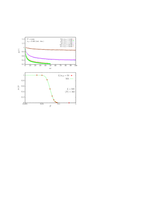
Figure 1: (Color online) Upper frame: WA first order correlation function $g_{1}(r)$ (one-body density matrix) as a function of $nr$ for several parameters $n|a_{1D}|$ compared to results from Astrakharchik and Giorgini (AG) G. E. Astrakharchik, J. Boronat, J. Casulleras, and S. Giorgini (2005) for values of $n|a_{1D}|$ which are almost identical to the WA ones. The system is a 1D homogeneous Bose gas at a temperature of $\widetilde{T}=0.001$. Here $n$ is the average linear density and $a_{1D}$ the 1D scattering length. For the WA we have: $n|a_{1D}|=0.303$ (open circles), 1.003 (open up triangles), and 29.320 (stars), respectively. The corresponding data from AG are for almost the same $n|a_{1D}|$: 0.300 (solid circles), 1.000 (solid up triangles), and 30.000 solid down triangles, respectively. $\widetilde{T}$ is in units of the transition temperature $T_{d}$ and the initial density of the simulation is $n_{0}=0.4$. Lower frame: Superfluid fraction $\rho_{s}/\rho$ as a function of temperature $\widetilde{T}$. The system is again a 1D homogeneous gas of Bosons. The scattering length is $a_{1D}/L=1/50$, the length of the system is $L/a_{1D}=50$ and the thermodynamic average of the number of particles is $\langle N\rangle=302$. The solid circles are the WA results whereas the solid line is an analytical calculation using Eq.(18) of Del Maestro and Affleck Adrian Del Maestro and Ian Affleck (2010) with the same parameters as ours (see text).

III Tests of the WA code

In this section the WA code Pro is tested on a uniform interacting Bose gas in the absence of any trapping potential. First, it is verified that the code produces the OBDM properly via a comparison with previous results. Second, it is confirmed that for suitably chosen parameters, the temperature of the simulations is low enough to obtain a significant superfluid fraction $\rho_{s}/\rho$. In this respect, WA results for $\rho_{s}/\rho$ as a function of $\widetilde{T}$ were found to exactly match an analytical calculation. In another decisive program check, although this is implied in the subsequent Sec. IV.1, the SG transition originally observed by Haller et al. Elmar Haller, Russel Hart, Manfred J. Mark, Johann G. Danzl, Lukas Reichsöllner, Mattias Gustavsson, Marcello Dalmonte, Guido Pupillo, and Hanns-Christoph Nägerl (2010) was reproduced by adding a shallow periodic 1D OL to the homogeneous Bose-gas system.

III.1 One-body density matrix

The upper frame of Fig. 1 displays the OBDM $g_{1}(r)$ as a function of $nr$ at various $n|a_{1D}|$ obtained from WA simulations for three of the homogeneous Bose-gas cases already considered by Astrakharchik and Giorgini (AG) G. E. Astrakharchik, J. Boronat, J. Casulleras, and S. Giorgini (2005). The values of $n|a_{1D}|$ range from the strongly to the weakly-interacting regime as $n|a_{1D}|$ is increased. One can see that the agreement is excellent.

III.2 Superfluid fraction

The lower frame of Fig. 1 displays a comparison between the superfluid fraction $\rho_{s}/\rho$ obtained by WA and that by the equation

$$\rho_{s}/\rho\,=\,1\,-\,u\left|\frac{\theta_{3}^{\prime\prime}(0,e^{-2\pi u})}{\theta_{3}(0,e^{-2\pi u})}\right|$$ (18)

that is the same as Eq.(16) of Ref.Adrian Del Maestro and Ian Affleck (2010); except that it is rescaled to our units. Here $u=1/(2\widetilde{T}\langle N\rangle)$, with $\widetilde{T}=T/T_{d}$, $\langle N\rangle\,=\,302$, and $L/a_{1D}=50$. $\theta_{3}$ is the Jacobi Theta function of the third kind given by

$$\theta_{3}(z,q)\,=\,\sum_{n=-\infty}^{+\infty}q^{n^{2}}\exp(i2nz),$$ (19)

and can be evaluated using WOLFRAM MATHEMATICA${}^{\textsuperscript{\textregistered}}$. The system is a weakly interacting, dilute, and uniform 1D Bose gas whose initial density was set to $n_{0}=0.2$ so that $T_{d}=0.5027$. The WA results match exactly those of the analytical Eq.(18) casting away all doubts about the accuracy of the WA code. Further, $\widetilde{T}=0.001$ is low enough to allow a significant value for $\rho_{s}/\rho$. The reader must be alerted, that the parameters used in this section and the previous one are only for the purpose of making the comparisons in Fig. 1. The rest of this paper uses the parameters of Sec. II.5 above.

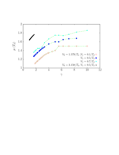
Figure 2: (Color online) Calibrated chemical potential $\mu$ as a function of $\gamma$ for the commensurate filling of a number of BCOLs with $\alpha=0.4$ and $\beta=1.0$ at $N=200\pm\delta$ particles, where $\delta$ is a small error. The figure displays the case for $V_{0}=1.579/T_{d}$ and $V_{1}=0.1/T_{d}$ (open circles); $0.5/T_{d}$ (solid circles); $0.7/T_{d}$ (solid up triangles); and then the case for $V_{0}=3.158/T_{d}$ and $V_{1}=0.5/T_{d}$ (solid down triangles). $\mu$ is in units of $T_{d}$ and $\gamma$ is unitless.

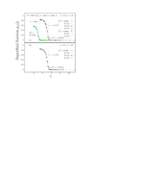
Figure 3: (Color online) WA superfluid fraction $\rho_{s}/\rho$ versus the Lieb-Liniger parameter $\gamma$ for an interacting Bose gas in several realizations of the BCOL. The figure demonstrates primarily the WA numerical reproduction of the Sine-Gordon transition observed experimentally in Ref.Elmar Haller, Russel Hart, Manfred J. Mark, Johann G. Danzl, Lukas Reichsöllner, Mattias Gustavsson, Marcello Dalmonte, Guido Pupillo, and Hanns-Christoph Nägerl (2010). The temperature of the system is $\widetilde{T}=0.001$, its length $L$ is such that $2L/\lambda=200$, and the number of particles $N$ is very close to 200 with a small error $\delta$ that is within the range $\pm 1$. Two primary OL depths $V_{0}^{(a)}=1.579/T_{d}$ and $V_{0}^{(b)}=3.158/T_{d}$ are considered with different associated depths $V_{1}^{(a)}$ and $V_{1}^{(b)}$ of the superimposed secondary OLs, respectively. Each of the primary OLs has exactly 200 sites with an occupancy of one particle per site in the SG regime. Upper frame ($a$) is for a QPOL with $\alpha=0.4$ and $\beta=1.0$. Open circles: $V_{1}^{(a)}=0.000$ (purely periodic OL); open up triangles: $0.1/T_{d}$; solid down triangles: $0.5/T_{d}$; and solid diamonds: $0.7/T_{d}$. Solid squares: $V_{1}^{(b)}=0.000$; stars: $0.5/T_{d}$; and crosses: $0.7/T_{d}$. Lower frame ($b$) is for a quasidisordered OL with $V_{0}^{(c)}=1.579/T_{d}$, the same $\alpha$, but a different $\beta=1.39$. The labels for $V_{1}^{(c)}$ are the same as for $V_{1}^{(a)}$. The vertical dashed lines show the SG transition points $\gamma=3.175$ for $V_{0}^{(a)}=V_{0}^{(c)}=1.579/T_{d}$, and $1.506$ for $V_{0}^{(b)}=3.158/T_{d}$ which are very close to the ones found on the phase diagram Fig.3 of Haller et al. Elmar Haller, Russel Hart, Manfred J. Mark, Johann G. Danzl, Lukas Reichsöllner, Mattias Gustavsson, Marcello Dalmonte, Guido Pupillo, and Hanns-Christoph Nägerl (2010). $V_{0}$, $V_{1}$, and $\widetilde{T}$ are in units of $T_{d}$ and $\gamma$ is unitless.

III.3 Chemical potential and interactions

In the simulations below, the number of particles $N$ for each $\gamma$ was fixed extremely close to 200 by a careful tuning of the chemical potential $\mu$ from a calibration curve, i.e., a plot of $N$ versus $\mu$ for each interaction strength $\gamma$. The error bars $\delta$ in $N$ were within $\pm 1.0$ and this error is unavoidable as one is dealing with a continuous-space Monte Carlo simulation. Fig. 2 displays a plot of the calibrated $\mu$ versus $\gamma$ for a number of BCOL realizations. The $\mu$ rises in general with $\gamma$ until it begins to stabilize in the strongly-interacting SG regime.

IV Results

IV.1 Sine-Gordon transition

An important result of this work is that the WA is able to reproduce the SG transition Elmar Haller, Russel Hart, Manfred J. Mark, Johann G. Danzl, Lukas Reichsöllner, Mattias Gustavsson, Marcello Dalmonte, Guido Pupillo, and Hanns-Christoph Nägerl (2010) in a primary 1D shallow periodic OL. It is found that the latter transition is robust against perturbations arising from the addition of a weaker secondary OL. The critical value $\gamma_{c}$ at which the transition occurs in a BCOL (1) remains exactly the same as compared to a periodic OL with the same $V_{0}$, unaffected by the latter perturbations. This is the chief result of this paper and is demonstrated by the behavior of $\rho_{s}/\rho$ as a function of $\gamma$ for a Bose gas in various realizations of a 1D BCOL (1). Fig. 3 demonstrates this finding for two values of the primary depth $V_{0}^{(a)}$ and $V_{0}^{(b)}$ and different strengths of the associated secondary OL, $V_{1}^{(a)}$ and $V_{1}^{(b)}$, respectively. Here, $\rho_{s}/\rho$ displays a steep decline towards the critical $\gamma_{c}$ beyond which it remains zero deep into the SG regime $\gamma\gg\gamma_{c}$. The value of $\gamma_{c}$ indicated by a vertical dashed line is obtained by fitting a function of the form $f(\gamma)\,=\,A(\gamma-\gamma_{c})^{s}$ to the data of $\rho_{s}/\rho$ in a narrow range of $\gamma$ where $\rho_{s}/\rho$ comes close to zero. Here $A$, $\gamma_{c}$, and $s$ are fitting parameters. We shall return to this issue in a future publication where a comparison between WA numerical and experimental results is required in order to explore the validity of the SG theory Grigory E. Astrakharchik, Konstantin V. Krutitsky, Maciej Lewenstein, and Ferran Mazzanti . The addition of a secondary OL does not alter the behavior of $\rho_{s}/\rho$ from the one observed for $V_{1}^{(a,b,c)}=0$, the purely periodic OL. For $V_{0}^{(c)}\,=\,1.579/T_{d}$, the behavior of $\rho_{s}/\rho$ in frame ($b$) with $\beta/\alpha=3.475$ is exactly the same as in frame ($a$) with $\beta/\alpha=2.5$ and the same $V_{0}^{(a)}\,=\,1.579/T_{d}$. This is a rather peculiar result showing that an increased quasidisorder [cf. Eq.(5) with $\epsilon=\beta/\alpha$] in a shallow BCOL does not alter the behavior of $\rho_{s}/\rho$. The values of $\gamma_{c}$ at which the transitions occur for both values of $V_{0}$ are very close to the ones obtained from the phase diagram in Fig. 3 of Haller et al. Elmar Haller, Russel Hart, Manfred J. Mark, Johann G. Danzl, Lukas Reichsöllner, Mattias Gustavsson, Marcello Dalmonte, Guido Pupillo, and Hanns-Christoph Nägerl (2010). This is again a striking demonstration of the fact that the WA is a powerful method enabling an accurate simulation of the behavior of lattice bosons in continuous space.

The robustness of $\rho_{s}/\rho$ against the secondary-OL perturbations arises because the particles always seek the lowest energy states of the BCOL, i.e., those of the primary OLs. Further, in the strongly-interacting regime $\gamma>1$, the interactions override the effects introduced by $V_{1}$ as the behavior of bosons is chiefly dictated by the commensurate filling of the primary OL. This finding is brought in line with that of Boeris et al. G. Bo$\acute{e}$ris, L. Gori, M. D. Hoogerland, A. Kumar, E. Lucioni, L. Tanzi, M. Inguscio, T. Giamarchi, C. D’Errico, G. Carleo, G. Modugno, and L. Sanchez-Palencia (2016), who argued that in the limit of a shallow periodic potential the optical depth becomes subrelevant when the Mott transition is only controlled by interactions.

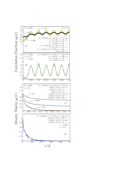
Figure 4: (Color online) Effect of secondary optical lattice on the spatially-averaged correlation function $g_{2}(r)$ [Eq.(9)] and the spatially-averaged density matrix $g_{1}(r)$ [Eq.(15)] of the systems in Fig. 3. Here $r$ is the distance between any pair of particles along the lattice and all frames share the same $x-$axis label. Frame ($A$) shows $g_{2}(r)$ for $\alpha=0.4$ at different interaction strengths and for various BCOL realizations. For $\gamma=2.500$, $V_{0}=1.579/T_{d}$, and $\beta=1$, the figure displays the cases for: $V_{1}=0.1/T_{d}$ (solid line); $0.5/T_{d}$ (long-dashed line); $0.7/T_{d}$ (short-dashed line); $1.0/T_{d}$ (fine-dotted line). (It is difficult to plot these lines so that all symbols can be distinguished from each other because they’re exactly overlapping. The same applies to the rest of the plots.) For $\gamma=1.724$, $V_{0}=3.158/T_{d}$, and the same $\beta$, the figure shows the cases for $V_{1}=0.0$ (solid circles) and $0.5/T_{d}$ (dashed-dotted line). The last set of data is for $\gamma=0.5$, $V_{0}=1.579/T_{d}$ but with $\beta=1.39$ and: $V_{1}=0.5/T_{d}$ (double-dotted line) and $1.0/T_{d}$ (open circles). Frame ($B$) is as in ($A$); except for $V_{0}=6.316/T_{d}$, $\gamma=0.833$, and: $V_{1}=1.0/T_{d}$ with $\beta=1.39$ (dashed double-dotted line); $3.0/T_{d}$ with 1.39 (long-dashed line); $1.0/T_{d}$ with 1.0 (short-dashed line); and $3.0/T_{d}$ with 1.0 (fine-dotted line). Going over to $g_{1}(r)$, frame ($C$) displays it for $\gamma=2.500$, $V_{0}=1.579/T_{d}$, and: $V_{1}=0.1/T_{d}$ with $\beta=1.0$ (solid line); $0.5/T_{d}$ and 1.0 (dashed line); $1.0/T_{d}$ and 1.0 (dotted line). The following set of data is for $\gamma=1.724$, $V_{0}=3.158/T_{d}$ and: $V_{1}=0.000$ with $\beta=1.0$ (fine-dotted line); $0.5/T_{d}$ with $\beta=1.0$ (dashed double-dotted line). Next comes $V_{0}=1.579/T_{d}$, $\gamma=0.5$, and $V_{1}=0.5/T_{d}$ with $\beta=1.39$ (dashed-dotted line); $1.0/T_{d}$ and 1.39 (double-dotted line). Finally, frame ($D$) is as in ($C$); except for $V_{0}=6.316/T_{d}$, $\gamma=0.833$, and: $V_{1}=1.0/T_{d}$ with $\beta=1.39$ (dashed double-dotted line); $3.0/T_{d}$ and 1.39 (dashed line); $1.0/T_{d}$ and 1.0 (solid line); $3.0/T_{d}$ and 1.0 (dashed-dotted line). The $r$ is in units of $L$, $\widetilde{T}$ is in units of $T_{d}$, and $\gamma$ is unitless.

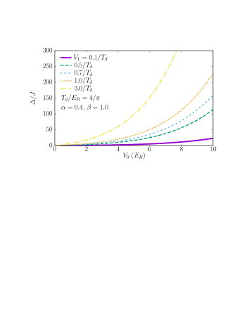
Figure 5: (Color online) $\Delta/J$ [given by Eqs.(5) and (6)] as a function of the primary OL depth $V_{0}$ for various values of $V_{1}$: $0.1/T_{d}$ (solid line); $0.5/T_{d}$ (long-dashed line); $0.7/T_{d}$ (short-dashed line); $1.0/T_{d}$ (dotted line); and $3.0/T_{d}$ (dashed double-dotted line). The conversion factor from units of $T_{d}$ to $E_{R}$ is $T_{d}/E_{R}=4/\pi$, $V_{0}$ is in units of $E_{R}$, and $\Delta/J$ is unitless.

Table 1: Ratio between the disorder strength $\Delta$ [Eq.(5)] and the tunneling amplitude $J$ [Eq.(6)] for various realizations of the BCOL. The table lists from left to right the primary OL depth $V_{0}$, the secondary one $V_{1}$, the parameters determining the periodicity of the BCOL (1), $\alpha$ and $\beta$, the parameters $\Delta$ and $J$, and then $\Delta/J$. The OL depths are in units of $T_{d}$, whereas $\Delta$ and $J$ are in units of $E_{R}$.

$V_{0}$	$V_{1}$	$\alpha$	$\beta$	$\Delta$	$J$	$\Delta/J$
($T_{d}$)	($T_{d}$)			($E_{R}$)	($E_{R}$)
1.579	0.1	0.4	1.0	0.0224	0.1804	0.1240
	0.5			0.1119	0.1804	0.6200
	0.7			0.1566	0.1804	0.8679
	0.1		1.39	0.0432	0.1804	0.2395
	0.5			0.2161	0.1804	1.1977
	0.7			0.3026	0.1804	1.6768
3.158	0.5		1.0	0.2349	0.1510	1.5553
	0.7			0.3288	0.1510	2.1775
6.316	1.0			0.7662	0.0886	8.6495
	3.0			2.2987	0.0886	25.948
	1.0		1.39	1.4805	0.0886	16.712
	3.0			4.4414	0.0886	50.135

IV.2 Effect of secondary lattice

Figure 4 shows the influence of $V_{1}$ on the spatial behavior of $g_{1}(r)$ and $g_{2}(r)$, particularly the amplitudes of the $g_{2}(r)-$oscillations, for various realizations of the BCOL. A significant feature is that $g_{2}(r)$ reveals a spatial oscillatory structure whose origin can be traced back to the primary OL. On the other hand, $g_{1}(r)$ in ($C$) displays a structure similar to $g_{1}(r)$ of the 1D homogeneous Bose gas in Fig. 1 without any spatial oscillations.

As $V_{0}$ is increased, so do the oscillatory amplitudes of $g_{2}(r)$ in ($B$) displaying its deep connection to the OL. An enhanced spatial decay rate of $g_{1}(r)$ at larger $V_{0}$ in ($C$) indicates a reduction of the superfluid fraction. The spatial frequency of the $g_{2}(r)-$oscillations neither changes with $V_{0}$ nor with $V_{1}$, and is largely governed by the lattice parameter of the primary OL. When $V_{0}$ and $V_{1}$ are small, e.g. $\sim 1.5/T_{d}$ in frames (A) and (C), a change of $V_{1}$ does not alter the spatial behavior. Remarkably, the secondary OL is practically not “seen” by the bosons in this case. The $g_{1}(r)$ and $g_{2}(r)$ for bosons in a QPOL ($\beta=1.0$) do not differ from those in a QDOL ($\beta=1.39$). However, when $V_{0}$ is increased to larger values $\sim 6/T_{d}$ as in ($B$) and ($D$), a change in the band structure of the BCOL via $V_{1}$ and $\beta$ begins to assert itself in $g_{2}(r)$ and $g_{1}(r)$. Further, at larger $V_{0}=6.316/T_{d}$, the change in the oscillatory amplitude of $g_{2}(r)$ with $V_{1}$ is more pronounced for a QPOL than for a QDOL indicating that an increased disorder does not necessary yield a stronger response to $V_{1}$. The same argument can be applied to $g_{1}(r)$ in frame (D). The secondary OL begins to influence the properties only in conjunction with a larger $V_{0}$ at which the BCOL begins to compete with the boson-boson interactions. Indeed, the difference in $\beta/\alpha$ introduces a difference between the band structures of the QPOL and the QDOL and therefore the corresponding $g_{2}(r)$.

One can also explain the stronger response to $V_{1}$ by examining $\Delta/J$ for a noninteracting Bose gas in a BCOL. A plot of $\Delta/J$ [cf. Eqs.(5) and (6)] as a function of $V_{0}$, shows that $\Delta/J$ increases significantly at the larger $V_{1}$. Naturally, according to Eq.(5), $\Delta$ rises with $\epsilon$ and $V_{1}$. Fig. 5 demonstrates these facts for a number of $V_{1}$ values and for $\alpha=0.4$ and $\beta=1.0$ only. In addition, Table 1 lists $\Delta/J$ for the various realizations of the BCOL in the present work. It can be seen for example that for $V_{0}=6.316/T_{d}$ and $\beta=1.39$, $\Delta/J$ begins to attain values that are much larger than for the rest of the BCOL parameters. As such, the properties of the system should begin to change significantly at this $V_{0}-$height. For the other OL depths and $\beta-$values, $\Delta/J$ has relatively small values of the order of $\sim 1$, and therefore, the secondary OL is unable to cause any changes in the properties.

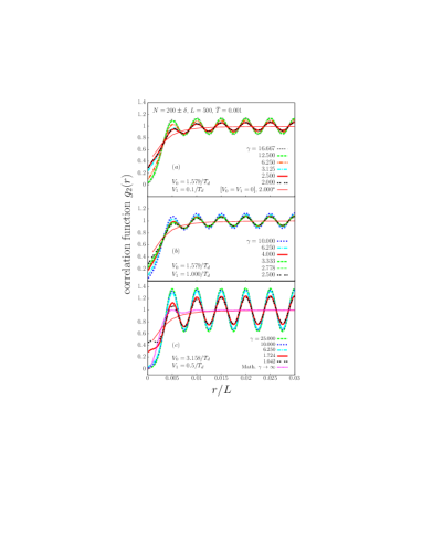
Figure 6: (Color online) WA pair correlation function $g_{2}(r)$ [Eq.(9)] at various interactions $\gamma$ for the systems of Fig. 3($a$) and three realizations of the BCOL with $\alpha=0.4$ and $\beta=1.0$. Frame ($a$) is for the BCOL of primary depth $V_{0}=1.579/T_{d}$ and a secondary depth $V_{1}=0.1/T_{d}$ at $\gamma=16.667$ (dotted line); 12.500 (dashed line); 6.250 (dashed triple-dotted line); 3.125 (dashed-dotted line); 2.500 (thick solid line); and 2.000 (double-dotted line). For additional comparison, the thin solid line is exceptionally displayed for a homogeneous Bose gas without an OL [$V_{0}=V_{1}=0$] at $\gamma=2.000$ and the same parameters as in Fig. 3($a$). It is also displayed in frames ($b$) and ($c$). Frame ($b$) is as in ($a$); but for $V_{1}=1.0/T_{d}$ and $\gamma=10.000$ (dotted line); 6.250 (dashed-dotted line); 4.000 (thick-solid line); 3.333 (dashed line); 2.778 (thin-dashed line); 2.500 (double dotted line). Frame ($c$) is for $V_{0}=3.158/T_{d}$, $V_{1}=0.5/T_{d}$, and: $\gamma=25.000$ (dashed line); 10.000 (dotted line); 6.250 (dashed-dotted line); 1.724 (thick solid line); 1.042 (double-dotted line). The fine-dotted line shows the pair correlation function. The thin-dashed and thin-dashed-dotted lines show the analytic results $g_{2}^{(per)}(z,1/\gamma)$ with $z=n\pi r$ [Eq.(22)] at $\gamma=10$ and $g_{2}^{(per)}(r,\sqrt{\gamma})$ [Eq.(23)] at $\gamma=0.1$ from Ref.A. G. Sykes, D. M. Gangardt, M. J. Davis, K. Viering, M. G. Raizen, and K.V. Kheruntsyan (2008). The plot for these functions was generated by Mathematica^®. There is almost perfect commensurate filling with $N=200\pm\delta$ particles, where $\delta$ is a small error in the range $\pm 1$. $V_{0}$, $V_{1}$, and $\widetilde{T}$ are in units of $T_{d}$, and $\gamma$ is unitless.

IV.3 Effect of interactions on the correlations

Fig. 6 demonstrates the effect of interactions on $g_{2}(r)$ for all realizations of the BCOL. The qualitative pattern of these oscillations hardly changes with $\gamma$ (and $V_{1}$), even on going through the SG transition. Quantitatively, however, the amplitude of these oscillations rises in general in response to an increase of $\gamma$ (and $V_{0}$). [Compare frame $(c)$ with both $(a)$ and $(b)$.] The latter manifests an increase in the interplay between the interactions and the BCOL that in turn enhances the boson-boson (i.e., density-density $n_{c}(r)$) correlations. It must be emphasized that the rise in the amplitude of $g_{2}(r)-$oscillations is particularly significant beyond $\gamma_{c}$ reaching deep into the SG regime where the bosons are pinned. This is therefore indicative of a Mott insulator (MI) state which is not inert. An examination of the MGF $G(p=0,\tau)$ in Sec. IV.7 and by making connections to $g_{2}(r)$, it is inferred that holes, arising from particle-hole (p$-$h) excitations, play an important role in the enhancement of $g_{2}(r)$.

On the one hand, the response of $g_{2}(r)$ to $\gamma$ can be further clarified by other arguments. First, it is known that $g_{2}(r)$ [Eq.(9)] describes the probability of finding two particles at a separation $r$. Hence, as the bosons become more localized with increasing $\gamma$, the probability –i.e., the amplitude of $g_{2}(r)-$oscillations– rises. Second, when the interactions are large, higher harmonics in the density operator $\widetilde{\rho}(x)$ from Ref.T. Giamarchi (2003) become excited that play a role in intensifying $g_{2}(r)$. Here, $\psi(x)=\sqrt{\widetilde{\rho}(x)}\exp(i\varphi(x))$ is a field operator with $\varphi(x)$ a phase and T. Giamarchi (2003); G. Roux, T. Barthel, I. P. McCulloch, C. Kollath, U. Schollwöck, and T. Giamarchi (2008)

$$\widetilde{\rho}(x)~{}=~{}$$

$$\left\{n^{2}+\frac{1}{\pi^{2}}[\nabla\phi(x)]^{2}+n^{2}\sum_{p>1}\cos(2\pi nx-2p\phi(x))\right\}^{1/2}$$

(20)

where $\phi(x)$ is a boson field operator and $n$ the average density. On the other hand, the rise in the amplitude with $V_{0}$ can be related to the amplitude of the Wannier state in each OL well. For sufficiently deep OLs, the Wannier state can be approximated by a harmonic oscillator ground state D. J. Boers, B. Goedeke, D. Hinrichs and M. Holthaus (2007)

$$W(x)~{}=~{}\frac{k^{1/2}}{\pi^{1/4}}\left(\frac{V_{0}}{E_{r}}\right)^{1/8}\exp\left[-\frac{1}{2}\left(\frac{V_{0}}{E_{r}}\right)^{1/2}k^{2}x^{2}\right]$$ (21)

where $k$ is the primary lattice wavevector. The amplitude of $W(x)$ rises with $V_{0}$ at each lattice site and consequently the amplitude of $g_{2}(r)$. Moreover, it has been found Alexander Yu. Cherny and Joachim Brand (2009), that correlations arise from the interplay of quantum statisics, interactions, thermal, and quantum fluctuations, the last of which can be related to the higher harmonics in Eq.(20).

IV.4 Another test of the WA for $g_{2}(r)$

For the homogeneous Bose gas, we display in Fig. 6($c$) the analytic result for $g_{2}(r)$ perturbative in $1/\gamma$ A. G. Sykes, D. M. Gangardt, M. J. Davis, K. Viering, M. G. Raizen, and K.V. Kheruntsyan (2008)

$$g_{2}^{(per)}(z,1/\gamma)=1-\frac{\sin^{2}z}{z^{2}}-\frac{4}{\gamma}\frac{\sin^{2}z}{z^{2}}-\frac{2\pi}{\gamma}\frac{\partial}{\partial z}\frac{\sin^{2}z}{z^{2}}+$$

$$\frac{2}{\gamma}\frac{\partial}{\partial z}\left[\frac{\sin^{2}z}{z^{2}}\int_{-1}^{1}dt\,\sin(zt){\rm ln}\frac{1+t}{1-t}\right]$$ (22)

where $z=n\pi r$ and the one perturbative in $\gamma$

$$g_{2}^{(per)}(r,\sqrt{\gamma})=1-\sqrt{\gamma}\left[{\rm L}_{-1}\left(2\sqrt{\gamma}nr\right)-{\rm I}_{1}\left(2\sqrt{\gamma}nr\right)\right],$$ (23)

where, ${\rm L_{-1}}(x)$ and ${\rm I}_{1}(x)$ are the Struve and Bessel functions, respectively. Eq.(22) is plotted with $\gamma=10$ for the strongly, whereas (23) with $\gamma=0.1$ for the weakly interacting regime. The goal is to check the WA $g_{2}(r)$ [e.g. for $\gamma=2.000$] without an OL against analytic calculations, and one can see that the WA result lies largely intermediate between these analytic results. This shows again that WA is reliable in calculating these properties.

IV.5 Origin of oscillations

Despite the fact that (22) diplays weak oscillations, these are substantially enhanced in the WA $g_{2}(r)$ by the addition of an OL. The WA $g_{2}(r)$ for the Bose gas without an OL does not show any oscillations whatsoever [e.g. for $\gamma=2.000$ and no OL in Fig. 6]. It is known that strongly-repulsive bosons in 1D without an OL arrange themselves in a periodic structure as if they were ordered inside an OL, but still the $g_{2}(r)$ reveals no spatial oscillations. Fact is, that the OL introduces a different energy level structure that reshapes the wavefunction into a spatially oscillatory form.

Let us here only mention briefly the results of the appendices and the reader is referred to the them for more information. In Appendix B, the SAPCF $h_{2}(r)$ [Eq.(14)] and the SA-OBDM $h_{1}(r)$ [Eq.(16)] are displayed in Figs. 9 and 10 (for the same systems of Figs. 4 and 6, respectively). The goal is to reveal the effects introduced into the correlations when instead of $n_{0}^{2}$ and $n_{0}$, the $g_{2}(r)$ and $g_{1}(r)$ are normalized by $\rho_{c}(r)$ and $\rho_{c,\frac{1}{2}}(r)$ [Eq.(13) and (17)], respectively. [That is $g_{1}(r)\rightarrow h_{1}(r)=g_{1}(r)n_{0}/\rho_{c,\frac{1}{2}}(r)$ and $g_{2}(r)\rightarrow h_{2}(r)=g_{2}(r)n_{0}^{2}/\rho_{c}(r)$.] The result is that in general –for a shallow BCOL– $h_{2}(r)$ displays oscillations with a (much) smaller amplitude than $g_{2}(r)$. In fact for a shallow BCOL, $h_{2}(r)$ is seen to approach the behavior of $g_{2}(r)$ for a homogeneous Bose gas! It can therefore be concluded, that in this case the origin of the $g_{2}(r)-$oscillations is the oscillations in the spatial density whose structure is determined by the OL. In Appendix B, except for small oscillations, $h_{1}(r)$ shows generally the same qualitative behavior as $g_{1}(r)$.

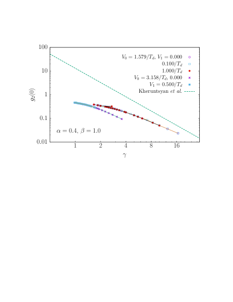
Figure 7: (Color online) Spatially-averaged WA local pair correlation function $g_{2}(r=0)$ [Eq.(9)] as a function of $\gamma$ for the systems of Fig. 6 in comparison to $g^{(2)}(\gamma)$ of Kheruntysan et al. K. V. Kheruntsyan, D. M. Gangardt, P. D. Drummond, and G. V. Shlyapnikov (2003) (dashed line) for the homogeneous Bose gas in the strongly interacting regime $\gamma>1$. Here, the QPOL is with $\alpha=0.4$ and $\beta=1.0$. The figure displays $g_{2}(0)$ for $V_{0}=1.579/T_{d}$ with $V_{1}=0$ (open circles); with $V_{1}=0.100/T_{d}$ (open squares); and with $V_{1}=1.000/T_{d}$ (solid circles). The stars are for $V_{0}=3.158/T_{d}$ with $V_{1}=0.000$ and with $V_{1}=0.5/T_{d}$ (solid squares).

IV.6 Interaction energy and local $g_{2}(0$)

According to Astrakharchik et al. G. E. Astrakharchik, J. Boronat, J. Casulleras, and S. Giorgini (2005), the total interaction energy $E_{int}$ can be computed from $g_{2}(r)$ at $r=0$ using

$$\frac{E_{int}}{\langle N\rangle T_{d}}\,=\,\frac{1}{2}g_{1D}ng_{2}(0).$$ (24)

Now $E_{int}$ goes to zero as $\gamma$ is increased to large values beyond $\gamma_{c}$ because $g_{2}(0)\rightarrow 0$. This can be seen in Fig. 6 for $\gamma>6.250$ in all frames and is a stark indication to fermionization of the bosons K. V. Kheruntsyan, D. M. Gangardt, P. D. Drummond, and G. V. Shlyapnikov (2003) and demonstrates perfect antibunching A. G. Sykes, D. M. Gangardt, M. J. Davis, K. Viering, M. G. Raizen, and K.V. Kheruntsyan (2008). In frame ($c$), fermionization is reached at $\gamma=10$ whereas in frames ($a$) and ($b$) it requires $\gamma>10$. Therefore, a larger $V_{0}$ aids the fermionization process of bosons since there is an enhanced effective interaction arising from the interplay between the BCOL and the repulsive forces that reduces the value of $\gamma$ required for fermionization. The added secondary OL does not play a role in this regard.

In Fig. 7, $g_{2}(0)$ is plotted as a function of $\gamma$ for the two BCOLs with $V_{0}=1.579/T_{d}$ and $3.158/T_{d}$ and some values of $V_{1}$. For comparison, the analytical result for the homogeneous Bose gas of Ref.K. V. Kheruntsyan, D. M. Gangardt, P. D. Drummond, and G. V. Shlyapnikov (2003),

$$g^{(2)}(\gamma)=\frac{4}{3}\frac{\pi^{2}}{\gamma^{2}}\left[1+\frac{t^{2}}{4\pi^{2}}\right],$$ (25)

with $t=T/T_{d}$ is displayed by the linear dashed line. It is immediately observed that, whereas on the one hand the introduction of an OL to a homogeneous Bose gas reduces $E_{int}$ via a significant reduction of $g_{2}(0)$, the addition of a secondary weaker OL does not play much of a role in changing the behavior of $g_{2}(0)$ for the same $V_{0}$. The interaction in the system is therefore not influenced by a perturbation of the primary OL. The effect of $\gamma$ on $g_{1}(r)$ shall be explored in a future publication in connection to the change of its behavior across the SG transition.

In Appendix D, $h_{2}(0)$ vs $\gamma$ is displayed in Fig. 11 for the same systems of Fig. 7. Peculiarly, $h_{2}(0)$ shows qualitatively the same behavior of $g_{2}(0)$.

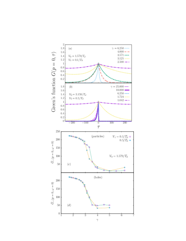
Figure 8: (Color online) WA Matsubara Green’s function $G(p=0,\tau)$ and weights of particle and hole (p-h) excitations $\widetilde{G}_{+}(p=0,\omega=0)$ and $\widetilde{G}_{-}(p=0,\omega=0)$ [Eq.(LABEL:eq:FTG+G-)], respectively, for the systems of Fig. 3. Upper figure displays $G$ as a function of $\tau$ for some values of $\gamma$, and the lower $\widetilde{G}_{\pm}$ as a function of $\gamma$ –all for different values of $V_{1}$. Frame ($a$) displays $G$ for $V_{0}=1.579/T_{d}$ and $V_{1}=0.100/T_{d}$ with: $\gamma=6.250$ (dotted line); 4.000 (double-dotted line); 3.571 (dashed line); 3.125 (fine-dotted line); 2.500 (dashed triple-dotted line). Frame ($b$) is as in ($a$); but with $V_{0}=3.158/T_{d}$, $V_{1}=0.5/T_{d}$ and: $\gamma=25.000$ (dotted line); 10.000 (solid line); 6.250 (dashed line); 1.724 (fine-dotted line); 1.042 (dashed triple-dotted line). Frame ($c$) shows $\widetilde{G}_{+}$ for $V_{0}=1.579/T_{d}$ and $V_{1}=0.1/T_{d}$ (open circles); $0.5/T_{d}$ (solid circles). Frame ($d$) is as in ($c$) with the same labels; but for $\widetilde{G}_{-}$. $T$ and $\mu$ are in units of $T_{d}$ and $\gamma$ is unitless.

IV.7 Matsubara Green’s function

The MGF $G(p=0,\tau)$ displays (1) the presence of a gas of particle-hole (p-h) pairs revealing that the insulating state obtained following the SG transition is not inert similar to an MI Stefan S. Natu and Erich J. Mueller (2013) and (2) that the weight of p-h excitations declines with increasing $\gamma$. This is shown in Fig. 8 frames ($a$) and ($b$), where $G(p=0,\tau)$ decays at a faster rate with $|\tau|$ as $\gamma$ is increased for any realization of the BCOL (we show here only two cases). In the limit when $\tau\rightarrow\pm\infty$, one can approximate $G(p=0,\tau)$ by Maciej Lewenstein, Anna Sanpera, and Ver$\acute{o}$nica Ahufinger (2012)

$$G(p=0,\tau)\sim\left\{\begin{array}[]{l @{\quad;\quad} r}e^{-E_{P}t}&\tau\rightarrow+\infty\\ e^{+E_{H}t}&\tau\rightarrow-\infty\end{array}\right.$$ (26)

where $E_{P}$ and $E_{H}$ are the single-particle and single-hole excitation energies, and $\tau=it$ is imaginary time. $G(p=0,\tau)$ reveals that for larger $\gamma$ and $\tau$ higher values of $E_{P}$ and $E_{H}$ are required to induce p-h excitations. The life-time of the p-h excitations $\sim\hbar/E_{P}$ or $\sim\hbar/E_{H}$, respectively, declines therefore with increasing $\gamma$ as well. This demonstrates that because of the high repulsion the bosons become locked in their positions unable to move unless excited by a strong external perturbation. But even after they are excited, they are deexcited after a short time as they return to the OL. Moreover, $G(p=0,\tau)$ is asymmetric about the origin $\tau=0$, and particularly beyond the SG transition point $\gamma_{c}$, $G(p=0,\tau)$ displays higher probability for hole excitations than particles.

One can obtain a weight for the particle (hole) excitations from an integration of the area under $G(p=0,\tau)$ in the range $[0,\tau_{max}]$ ($[-\tau_{max},0]$), where $\tau_{max}=250$ is the maximum value of $\tau$. In fact, an integration from $-\tau_{max}$ to $+\tau_{max}$ would be approximately equivalent to the Fourier transform of $G(p=0,\tau)$ at a frequency of excitation $\omega=0$. We therefore consider for the present purpose

$$\widetilde{G}(p=0,\omega)\,\sim\,\int_{-\tau_{max}}^{+\tau_{max}}G(p=0,\tau)e^{-i\omega\tau}d\tau.$$ (27)

and separate it into two terms

$$\widetilde{G}(p=0,\omega)\,=\,\widetilde{G}_{+}(p=0,\omega)\,+\,\widetilde{G}_{-}(p=0,\omega),$$ (28)

where

$$\widetilde{G}_{+}(p=0,\omega)\, \sim \,\int_{0}^{\tau_{max}}G(p=0,\tau)e^{-i\omega\tau}d\tau,$$

$$\widetilde{G}_{-}(p=0,\omega)\, \sim \,\int_{-\tau_{max}}^{0}G(p=0,\tau)e^{-i\omega\tau}d\tau.$$

One can then define $\widetilde{G}_{+}(p=0,\omega=0)$ and $\widetilde{G}_{-}(p=0,\omega=0)$ as the weights of particle and hole excitations, respectively. $\omega=0$ is chosen because there is no excitation agent in our simulations.

Table 2: Standard deviation of the BCOL $\delta V$ [Eq.(2)] and $\Delta/J$ [cf. Eqs.(5) and (6)] for various realizations of the BCOL (1). From left to right the table lists the primary OL depth $V_{0}$, the secondary depth $V_{1}$, the standard deviation $\delta V$ for $\alpha=0.4$ and $\beta=1.39$, $\delta V$ for $\widetilde{\alpha}=0.401248...$ and $\widetilde{\beta}=1.389964...$, $\Delta/J$ for ($\alpha$,$\beta$), and finally $\Delta/J$ for ($\widetilde{\alpha}$,$\widetilde{\beta}$), respectively. $V_{0}$, $V_{1}$, $\delta V$ are in units of ($T_{d}$), and $\Delta/J$ is unitless.

$V_{0}$	$V_{1}$	$\delta V$ ($\alpha$,$\beta$)	$\delta V$ ($\widetilde{\alpha}$,$\widetilde{\beta}$)	$\Delta/J$	$\Delta/J$
($T_{d}$)	($T_{d}$)	($T_{d}$)	($T_{d}$)	($\alpha$,$\beta$)	($\widetilde{\alpha}$,$\widetilde{\beta}$)
1.579	0.1	0.5594	0.5595	0.2395	0.2380
	0.5	0.5856	0.5857	1.1977	1.1900
	0.7	0.6107	0.6108	1.6768	1.6600
6.316	1.0	2.2609	2.2613	16.712	16.6032
	3.0	2.4721	2.4726	50.138	49.8094

Frames ($c$) and ($d$) display $\widetilde{G}_{+}(0,0)$ and $\widetilde{G}_{-}(0,0)$ as functions of $\gamma$, for $V_{0}=1.579/T_{d}$ and some values of $V_{1}$. Obviously, $\widetilde{G}_{\pm}$ decline with increasing $\gamma$ and, moreover, both frames show an apparent change in the curvature of $\widetilde{G}_{\pm}$ close to the critical $\gamma_{c}$ at which the SG transition occurs. Therefore, the change in the sign of $\partial^{2}\widetilde{G}_{\pm}(0,0)/\partial\gamma^{2}$ is a signal for the SG transition, and $\partial^{2}\widetilde{G}_{\pm}(0,0)/\partial\gamma^{2}=0$ near $\gamma=\gamma_{c}$.

V Rational vs irrational $\lambda_{1}/\lambda_{2}$

Whereas the ratio $\beta/\alpha\,=\,\lambda_{1}/\lambda_{2}$ is clearly rational for both pairs of $(\alpha,\beta)=(0.4,1.0)$ and $(0.4,1.39)$, it could be argued that had one used for example the irrational values $\widetilde{\alpha}\,=\,\sqrt{0.161}\,=\,0.401248\cdots$ which is very close to 0.4, or $\widetilde{\beta}\,=\,\sqrt{1.9320}\,=\,1.389964\cdots$ close to 1.39, the same results would be gotten as for $(0.4,1.39)$. Within this context, Table 2 lists $\delta V$ [Eq.(2)] and $\Delta/J$ [Eqs.(5) and (6)] for various realizations of the BCOL at ($\widetilde{\alpha}$,$\widetilde{\beta}$) and the rational approximation ($\alpha$,$\beta$). It can be seen that the results of $\delta V$ and $\Delta/J$ for ($\alpha$,$\beta$) differ only slightly from that for ($\widetilde{\alpha}$,$\widetilde{\beta}$) by an order of magnitude $\stackrel{{\scriptstyle<}}{{\sim}}1\%$. In that sense, there should not be much difference in the results because of rational and irrational $\lambda_{1}/\lambda_{2}$.

VI Conclusion

In summary then, the properties of bosons in a shallow 1D bichromatic optical lattice (BCOL), with a rational ratio $\lambda_{1}/\lambda_{2}$ of its wavelengths, have been examined by scanning the system along a range of the Lieb-Liniger parameter $\gamma$ in the regime of the Sine-Gordon (SG) transition Elmar Haller, Russel Hart, Manfred J. Mark, Johann G. Danzl, Lukas Reichsöllner, Mattias Gustavsson, Marcello Dalmonte, Guido Pupillo, and Hanns-Christoph Nägerl (2010) at commensurate filling of the primary OL.

The chief result is that this transition in a primary OL of depth $V_{0}\sim 1.5/T_{d}$ is robust against the perturbations by a secondary OL of depth $V_{1}<V_{0}$. The critical interaction strength $\gamma_{c}$ at which the transition occurs remains the same as for the periodic OL. The corresponding behavior of the superfluid fraction $\rho_{s}/\rho$ vs $\gamma$ reveals absolutely no response to changes in $V_{1}$; this is quite the same for other properties such as the correlation function $g_{2}(r)$ and the one-body density matrix $g_{1}(r)$. In contrast, changes in the latter observables arise with $V_{1}$ for larger values of $V_{0}\sim 6/T_{d}$ at which the lattice-band structure of the primary OL begins to be influenced by the secondary OL.

However, for $V_{0}\sim 1.5/T_{d}$ the properties are significantly affected by changes in $\gamma$. In this regard, $g_{2}(r)$ demonstrates an oscillatory structure whose amplitude rises with $\gamma$ and $V_{0}$, manifestating an increase in the interplay between BCOL and interactions that yield the excitation of higher harmonics in the density operator. The origin of these oscillations lies chiefly in the primary OL. The latter changes are particularly significant beyond $\gamma_{c}$ reaching deep into the SG regime signalling the presence of a non-inert Mott insulator in the form of a particle-hole gas of bosons. At very large $\gamma$ beyond the critical $\gamma_{c}$, $g_{2}(0)\rightarrow 0$ signals fermionization and entrance to the Tonks-Girardeau regime. The fermionization process is aided by the primary OL and is unaffected by the secondary OL. Since $g_{2}(r)$ has been measured experimentally Toshiya Kinoshita, Trevor Wenger, and David S. Weiss (2005) over a broad range of the coupling strengths, our work should then motivate a future experimental measurement of $g_{2}(0)$ in a BCOL.

Although a division of $g_{2}(r)n_{0}^{2}$ and $g_{1}(r)n_{0}$ by the convoluted densities $\rho_{c}(r)$ and $\rho_{c,\frac{1}{2}}(r)$, respectively, yields qualitatively the same results as far as the sensitivity to changes in the BCOL is concerned, the response of $h_{2}(r)=g_{2}(r)n_{0}^{2}/\rho_{c}(r)$ to changes in $V_{0}$ and $\gamma$ is in general significantly weakened. Hence, $g_{2}(r)$ is more adequate for obtaining stronger signals of changes. The $g_{2}(r)$ displays oscillations arising from oscillations in the spatial density that account for the same behavior in the density-density correlations.

The MGF $G(p=0,\tau)$ displays a declining weight for the particle-hole excitations with rising $\gamma$ attributed to an increased localization of the bosons. Moreover, it has been found that the system favors hole excitations at strong interactions leading us to conclude that deep in the SG regime holes play a chief role in the response of $g_{1}(r)$ and $g_{2}(r)$ to $\gamma$. In addition, a change in the curvature of the Fourier transform of the MGF $G(p=0,\omega=0)$ as a function of $\gamma$ for either particles or holes, is a signal for the SG transition.

It has been particularly argued, that there shouldn’t be much difference between the results obtained by using an irrational $\lambda_{1}/\lambda_{2}$ and a rational approximation to the same $\lambda_{1}/\lambda_{2}$ basing on the fact that the disorder strength of a BCOL changes only by small percentages if one uses a rational approximation to, instead of an irrational, $\lambda_{1}/\lambda_{2}$.

Finally, it must be emphasized that the WA applied here has been tested for accuracy. By making comparions with previous results, it has been shown that the WA code works correctly and is therefore reliable. For example, our results for $g_{1}(r)$ are in very good agreement with those computed by Astrakharchik and Giorgini G. E. Astrakharchik, J. Boronat, J. Casulleras, and S. Giorgini (2005). Moreover, the superfluid behavior with temperature matches exactly an analytical calculation from Ref.Adrian Del Maestro and Ian Affleck (2010). Most importantly, the WA code was able to reproduce the SG transition observed earlier by Haller et al. Elmar Haller, Russel Hart, Manfred J. Mark, Johann G. Danzl, Lukas Reichsöllner, Mattias Gustavsson, Marcello Dalmonte, Guido Pupillo, and Hanns-Christoph Nägerl (2010). The current results are also in line with Edwards et al. E. E. Edwards, M. Beeler, Tao Hong, and S. L. Rolston (2008) who demonstrated that the effects of weak perturbations to a primary 1D OL disappear as interactions get stronger and we are in the strongly interacting regime. During the preparation of this paper, we learnt of an investigation bearing similarities to ours by Bo$\acute{e}$ris et al. G. Bo$\acute{e}$ris, L. Gori, M. D. Hoogerland, A. Kumar, E. Lucioni, L. Tanzi, M. Inguscio, T. Giamarchi, C. D’Errico, G. Carleo, G. Modugno, and L. Sanchez-Palencia (2016) where, among other issues, the WA has been applied to reproduce the SG transition, except that they only use a periodic OL with a different procedure than ours here.

Appendix A Worm Algorithm

Specifically, a WA code is applied which has been written by Nikolay Prokofev Pro originally for the simulation of 1D soft-core bosons without any trapping potential. A 3D version of this code, although for ⁴He on graphite, has been described earlier M. Boninsegni, N. V. Prokof’ev, and B. V. Svistunov (2006). WA is a path-integral Monte Carlo technique whose configurational space is extended to include what one calls “worms”. In this method, particles are described by Feynman’s path-integral formulation as closed trajectories in space-time (diagonal configurations). Each trajectory is a closed chain of “beads” and each “bead” is a pair of positions of the same particle separated by a time $\tau$ along the imaginary-time axis in space-time. In a closed trajectory, the initial and final positions of the path are the same along the space axis. The method considers imaginary “time” as inverse temperature G. D. Mahan (1990), i.e., $it/\hbar\leftrightarrow 1/(k_{B}T)$, where $\hbar$ is Planck’s constant, $k_{B}$ Boltzmann’s constant, and $T$ the temperature. The configuration of the system is updated by adding or removing open trajectories in space-time called “worms” (off-diagonal configurations) which are paths in space-time whose initial and final positions along the space axis are not the same. Therefore, the configuration of the system is divided into two sectors: the $Z-$sector containing all the closed trajectories and the $G-$sector containing one open trajectory, or worm. The code is designed to perform various updates on these worms via certain acceptance and rejection probabilities that are carefully weighted functions of, and including, the factors $\exp[-(\mathbf{r}_{\ell}\,-\,\mathbf{r}_{\ell-1})^{2}/(4\lambda\tau)]$ and $\exp[-\tau V(\mathbf{r}_{\ell})]$. Here $\lambda\,=\,\hbar^{2}/(2m)$ with $m$ the mass of a boson, $\tau\rightarrow 1/(Mk_{B}T)$ is the imaginary time step with $M$ the total number of beads constituting the particle’s trajectory along the imaginary time axis, $\mathbf{r}_{\ell}$ is the position of the $\ell^{th}$ bead along the space axis, and $V(\mathbf{r}_{\ell})$ is the potential energy of bead $\ell$. The above factors included in a worm-update probability are integrated along the time axis over the length of the worm being updated. The beginning and end of the worm are termed MASHA and IRA, respectively, where MASHA precedes IRA along the imaginary time axis. There are various types of updates: (1) INSERT or REMOVE in which a worm is created and added to, or annihilated from, the configuration, respectively; (2) MOVE FORWARD or MOVE BACKWARD that change the length of the worm in space-time along the imaginary time axis; (3) RECONNECT in which a worm is connected to a closed trajectory after opening it resulting in an exchange of particles (permutation); (4) CUT or GLUE where a closed trajectory is cut open by removing, or an open trajectory is closed by adding, a short chain of beads, respectively. All these updates are described in more detail by the inventors of the technique M. Boninsegni, N. V. Prokof’ev, and B. V. Svistunov (2006).

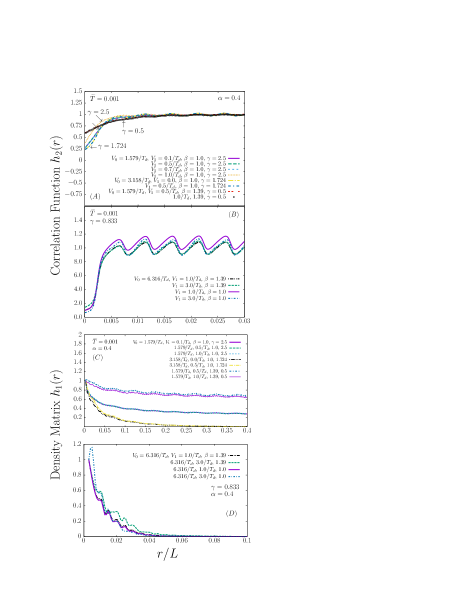
Figure 9: (Color online) As in Fig. 6; but for $h_{2}(r)$. Upper frame ($A$): at $\gamma=2.5$ and $V_{0}=1.579/T_{d}$ the figure displays the results for: $V_{1}=0.1/T_{d}$, $\beta=1.0$ (thick solid line); 0.5, 1.0 (thick-dashed line); 0.7, 1.0 (short-dashed line); 1.0, 1.0 (fine-dotted line). Then at $\gamma=1.724$ and $V_{0}=3.158/T_{d}$ the results for: 0.0, 1.0 (long-dashed dotted line); 0.5, 1.0 (short-dashed dotted line). At $\gamma=0.5$ and $V_{0}=1.579/T_{d}$ again the results are shown for: $V_{1}=0.5/T_{d}$, $\beta=1.39$ (double-dotted dotted line); 1.0, 1.39 (open circles). Upper frame ($B$) is for $V_{0}=6.316/T_{d}$, $\gamma=0.833$, and: $V_{1}=1.0/T_{d}$, $\beta=1.39$ (long-dashed double-dotted line); $3.0/T_{d}$, 1.39 (thick-dashed line); $1.0/T_{d}$, 1.0 (thin-dashed line); $3.0/T_{d}$, 1.0 (dashed-dotted line). Lower frame ($C$) is for the same system in ($A$); but for $h_{1}(r)$ with $V_{0}=1.579/T_{d}$ and: $V_{1}=0.1/T_{d}$, $\beta=1.0$, $\gamma=2.5$ (thick solid line); $0.5/T_{d}$, 1.0, 2.5 (thick-dashed line); $1.0/T_{d}$, 1.0, 2.5 (thin-dashed line). Then one has for $V_{0}=3.158/T_{d}$: $0.0/T_{d}$, 1.0, 1.724 (long-dashed double-dotted line); $0.5/T_{d}$, 1.0, 1.724 (dashed-dotted line). Next one has for $V_{0}=1.579/T_{d}$: $0.5/T_{d}$, 1.39, 0.5 (short-dashed dotted line); $1.0/T_{d}$, 1.39, 0.5 (thin solid line). Finally frame ($D$) is for the same system in ($B$); but for $h_{1}(r)$: dashed double-dotted line: $V_{1}=1.0/T_{d}$, $\beta=1.39$; dashed line: $3.0/T_{d}$, 1.0; thick solid line: $1.0/T_{d}$, 1.0; dashed-dotted line: $3.0/T_{d}$, 1.0.

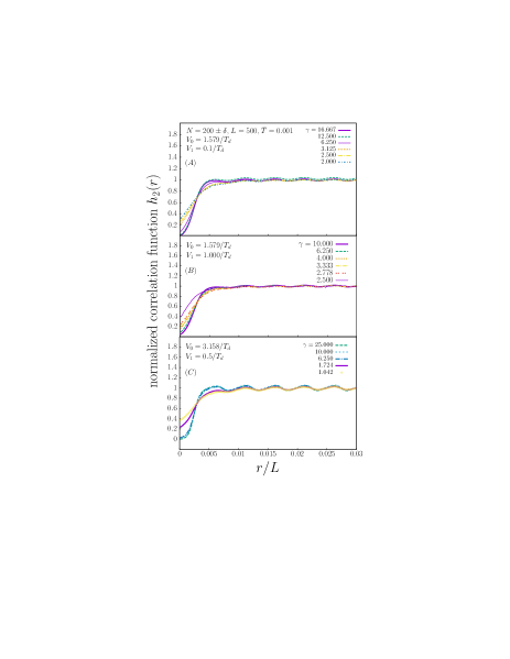
Figure 10: As in Fig. 6; but for $h_{2}(r)$. Frame ($A$): $V_{0}=1.579/T_{d}$, $V_{1}=0.1/T_{d}$ and: $\gamma=16.667$ (thick-solid line); 12.500 (dashed line); 6.250 (thin solid line); 3.125 (fine-dotted line); 2.500 (long-dashed dotted line); 2.000 (short-dashed dotted line). Frame ($B$) is for $V_{0}=1.579/T_{d}$, $V_{1}=1.000/T_{d}$ and: $\gamma=10.000$ (solid line); 6.250 (dashed line); 4.000 (fine-dotted line); 3.333 (dashed-dotted line); 2.778 (double-dotted line); 2.500 (thin solid line). Frame ($C$): $V_{0}=3.158$, $V_{1}=0.5/T_{d}$, and: $\gamma=25.000$ (thick-dashed line); 10.000 (thin-dashed line); 6.250 (dashed-dotted line); 1.724 (thick-solid line); 1.042 (circles).

Appendix B Pair correlation function for inhomogeneous 1D Bose gases

Fig. 9 is as in Fig. 4; but for $h_{2}(r)$ given by Eq.(14). In frame $(A)$ for low $V_{0}$, the amplitude of the spatial oscillations in $h_{2}(r)$ is substantially reduced compared to the corresponding $g_{2}(r)$. Although the $h_{2}(r)-$oscillations do not vanish completely, their amplitude does not change with $V_{1}$ that is the same for $g_{2}(r)$ in Fig. 4($A$). Indeed, the $g_{2}(r)-$oscillations are caused by the oscillations in the convoluted density $\rho_{c}(r)$ [Eq.(13)], and a division of $g_{2}(r)n_{0}^{2}$ by $\rho_{c}(r)$ [to get $h_{2}(r)$] almost flattens $h_{2}(r)$ at larger $r$ so that it oscillates close to 1. Any changes in the structure of $h_{2}(r)$ with $V_{1}$ are not detected. There is a weak role of the band structure of the BCOL and its disorder at low $V_{0}$ which is consistent with Fig. 5.

As one increases $V_{0}$ in Fig. 9($B$), the amplitude of oscillations in $h_{2}(r)$ rises similarly to $g_{2}(r)$. This time the normalization by $\rho_{c}(r)$ does not yield a significant suppression of the oscillations as it occurs in frame ($A$). Therefore, at larger $V_{0}$ the origin of these oscillations may not be anymore chiefly the oscillations in the spatial density; rather they largely arise from an increased effect of the band structure of the BCOL and the disorder; the latter is again consistent with the increase of disorder with $V_{0}$ in Fig. 5. Qualitatively nevertheless, Fig. 9 shows the same effects as Fig. 4, that is to say, that by either $g_{2}(r)$ or $h_{2}(r)$, one reaches qualitatively the same conclusions about the effect of $V_{1}$ on the strength of the correlations, namely that there is none at low $V_{0}$.

Fig. 10 is the same as Fig. 6; but for $h_{2}(r)$. Here, the effect of interactions $\gamma$ at $r\stackrel{{\scriptstyle>}}{{~{}}}0.00025$ is substantially weakened in by the division of $g_{2}(r)n_{0}^{2}$ by $\rho_{c}(r)$, but remains quite pronounced towards $r\rightarrow 0$. The effect of $\gamma$ at larger $r$ cannot therefore be significantly detected by $h_{2}(r)$ because the effect of interactions is absorbed by the normalization process. At $r=0$, $h_{2}(r)$ displays a reduction with $\gamma$ similar to Fig. 6 and shows the same decline as in Fig. 7 (see Sec.D below).

Appendix C One-body density matrix for inhomogeneous 1D Bose gases

The SA-OBDM $h_{1}(r)$ [Eq.(16)] in frames ($C$) and ($D$) of Fig. 9 displays qualitatively the same behavior as the corresponding $g_{1}(r)$, except for small oscillations that are a result of normalizing by $\rho_{c,\frac{1}{2}}(r)$. In fact, at larger $V_{0}$, there is really not much difference in the qualitative structure of $h_{1}(r)$ and $g_{1}(r)$ in frames ($D$) of Figs. 9 and 4, respectively $-$both of them display small oscillations. Therefore for larger $V_{0}$, $h_{1}(r)$ and $g_{1}(r)$ can both be applied on the same footage to draw conclusions about the superfluid depletion and role of the BCOL.

Appendix D Local correlation function for inhomogeneous 1D Bose gases

The SAPCF at $r=0$, i.e. $h_{2}(0)$, displays in Fig. 11 a drop with increasing $\gamma$ and shows almost the same behavior as $g_{2}(0)$ in Fig. 7. Again, changes in $V_{1}$ for the same $V_{0}$ have no effect on $h_{2}(0)$.

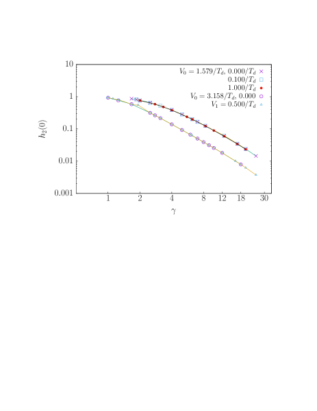
Figure 11: As in Fig. 7; but for $h_{2}(0)$ with $V_{0}=1.579/T_{d}$ and: $V_{1}=0$ (times); $0.1/T_{d}$ (open square); $1.0/T_{d}$ (solid circles). Next data is for $V_{0}=3.158$ and: $V_{1}=0$ (open circles) and $0.5/T_{d}$ (open triangles).

References

- P. Sengupta, M. Rigol, G. G. Batrouni, P. J. H. Denteneer, and R. T. Scalettar (2005) P. Sengupta, M. Rigol, G. G. Batrouni, P. J. H. Denteneer, and R. T. Scalettar, Phys. Rev. Lett. 95, 220402 (2005).
- Xia-Ji Liu, Peter D. Drummond, and Hui Hu (2005) Xia-Ji Liu, Peter D. Drummond, and Hui Hu, Phys. Rev. Lett. 94, 136406 (2005).
- S. R. Clark and D. Jaksch (2004) S. R. Clark and D. Jaksch, Phys. Rev. A 70, 043612 (2004).
- S. Ramanan, T. Mishra, M. S. Luthra, R. V. Pai, and B. P. Das (2009) S. Ramanan, T. Mishra, M. S. Luthra, R. V. Pai, and B. P. Das, Phys. Rev. A 79, 013625 (2009).
- Elmar Haller, Russel Hart, Manfred J. Mark, Johann G. Danzl, Lukas Reichsöllner, Mattias Gustavsson, Marcello Dalmonte, Guido Pupillo, and Hanns-Christoph Nägerl (2010) Elmar Haller, Russel Hart, Manfred J. Mark, Johann G. Danzl, Lukas Reichsöllner, Mattias Gustavsson, Marcello Dalmonte, Guido Pupillo, and Hanns-Christoph Nägerl, Nature 466, 597 (2010).
- H. P. Büchler, G. Blatter, and W. Zwerger (2003) H. P. Büchler, G. Blatter, and W. Zwerger, Phys. Rev. Lett. 90, 130401 (2003).
- T. Giamarchi (2003) T. Giamarchi, Quantum Physics in One Dimension (Oxford Univ. Press, 2003), 1st ed.
- Ming-Xia Huo and Dimitris G. Angelakis (2012) Ming-Xia Huo and Dimitris G. Angelakis, Phys. Rev. A 85, 023821 (2012).
- E. H. Lieb and W. Liniger (1963) E. H. Lieb and W. Liniger, Phys. Rev. 130, 1605 (1963).
- Guidoni et al. (1997) L. Guidoni, C. Triché, P. Verkerk, and G. Grynberg, Phys. Rev. Lett. 79, 3363 (1997).
- Nicolas Nessi and Anibal Iucci (2011) Nicolas Nessi and Anibal Iucci, Phys. Rev. A 84, 063614 (2011).
- M. C. Gordillo, C. Carbonell-Coronado, and F. De Soto (2015) M. C. Gordillo, C. Carbonell-Coronado, and F. De Soto, Phys. Rev. A 91, 043618 (2015).
- Mohammad Hafezi, Darrick E. Chang, Vladimir Gritsev, Eugene Demler, and Mikhail D. Lukin (2012) Mohammad Hafezi, Darrick E. Chang, Vladimir Gritsev, Eugene Demler, and Mikhail D. Lukin, Phys. Rev. A 85, 013822 (2012).
- Pethick and Smith (2002) C. J. Pethick and H. Smith, Bose-Einstein Condensation in Dilute Gases (Cambridge University Press, Cambridge UK, 2002), 1st ed.
- Maciej Lewenstein, Anna Sanpera, and Vernica Ahufinger (2012) Maciej Lewenstein, Anna Sanpera, and Vernica Ahufinger, Ultracold Atoms in Optical Lattices: Simulating Quantum Many-Body Systems (Oxford University Press, United Kingdom, 2012).
- G. Boris, L. Gori, M. D. Hoogerland, A. Kumar, E. Lucioni, L. Tanzi, M. Inguscio, T. Giamarchi, C. D’Errico, G. Carleo, G. Modugno, and L. Sanchez-Palencia (2016) G. Boris, L. Gori, M. D. Hoogerland, A. Kumar, E. Lucioni, L. Tanzi, M. Inguscio, T. Giamarchi, C. D’Errico, G. Carleo, G. Modugno, and L. Sanchez-Palencia, Phys. Rev. A 93, 011601(R) (2016).
- Toshiya Kinoshita, Trevor Wenger, and David S. Weiss (2005) Toshiya Kinoshita, Trevor Wenger, and David S. Weiss, Phys. Rev. Lett. 95, 190406 (2005).
- B. Deissler, E. Lucioni, M. Modugno, G. Roati, L. Tanzi, M. Zaccanti, M. Inguscio, and G. Modugno (2011) B. Deissler, E. Lucioni, M. Modugno, G. Roati, L. Tanzi, M. Zaccanti, M. Inguscio, and G. Modugno, New J. Phys. 13, 023020 (2011).
- G. Roux, T. Barthel, I. P. McCulloch, C. Kollath, U. Schollwöck, and T. Giamarchi (2008) G. Roux, T. Barthel, I. P. McCulloch, C. Kollath, U. Schollwöck, and T. Giamarchi, Phys. Rev. A 78, 023628 (2008).
- Tommaso Roscilde (2008) Tommaso Roscilde, Phys. Rev. A 77, 063605 (2008).
- M. Larcher, M. Modugno, and F. Dalfovo (2011) M. Larcher, M. Modugno, and F. Dalfovo, Phys. Rev. A 83, 013624 (2011).
- Michele Modugno (2009) Michele Modugno, New J. Phys. 11, 033023 (2009).
- R. Roth and K. Burnett (2003) R. Roth and K. Burnett, Phys. Rev. A 67, 031602(R) (2003).
- S. Pilati, S. Giorgini, M. Modugno, and N. Prokof’ev (2010) S. Pilati, S. Giorgini, M. Modugno, and N. Prokof’ev, New J. Phys. 12, 073003 (2010).
- I. L. Aleiner, B. L. Altshuler, and G. V. Shlyapnikov (2010) I. L. Aleiner, B. L. Altshuler, and G. V. Shlyapnikov, Nature Phys. 6, 900 (2010).
- P. Lugan, A. Aspect, L. Sanchez-Palencia, D. Delande, B. Grmaud, C. A. Müller, and C. Miniatura (2009) P. Lugan, A. Aspect, L. Sanchez-Palencia, D. Delande, B. Grmaud, C. A. Müller, and C. Miniatura, Phys. Rev. A 80, 023605 (2009).
- M. White, M. Pasienski, D. McKay, S. Q. Zhou, D. Ceperley, and B. DeMarco (2009) M. White, M. Pasienski, D. McKay, S. Q. Zhou, D. Ceperley, and B. DeMarco, Phys. Rev. Lett. 102, 055301 (2009).
- L. Fallani, J. E. Lye, V. Guarrera, C. Fort, and M. Inguscio (2007) L. Fallani, J. E. Lye, V. Guarrera, C. Fort, and M. Inguscio, Phys. Rev. Lett. 98, 130404 (2007).
- B. Deissler, M. Zaccanti, G. Roati, C. DÉrrico, M. Fattori, M. Modugno, G. Modugno, and M. Inguscio (2010) B. Deissler, M. Zaccanti, G. Roati, C. DÉrrico, M. Fattori, M. Modugno, G. Modugno, and M. Inguscio, Nature Phys. 6, 354 (2010).
- Giacomo Roati, Chiara DÉrrico, Leonardo Fallani, Marco Fattori, Chiara Fort, Matteo Zaccanti, Giovanni Modugno, Michele Modugno, and Massimo Inguscio (2008) Giacomo Roati, Chiara DÉrrico, Leonardo Fallani, Marco Fattori, Chiara Fort, Matteo Zaccanti, Giovanni Modugno, Michele Modugno, and Massimo Inguscio, Nature 453, 895 (2008).
- Juliette Billy, Vincent Josse, Zhanchun Zuo, Alain Bernard, Ben Hambrecht, Pierre Lugan, David Clment, Laurent Sanchez-Palencia, Philippe Bouyer, and Alain Aspect (2008) Juliette Billy, Vincent Josse, Zhanchun Zuo, Alain Bernard, Ben Hambrecht, Pierre Lugan, David Clment, Laurent Sanchez-Palencia, Philippe Bouyer, and Alain Aspect, Nature Phys. Lett. 453, 891 (2008).
- Yong P. Chen, J. Hitchcock, D. Dries, M. Junker, C. Welford, and R. G. Hulet (2008) Yong P. Chen, J. Hitchcock, D. Dries, M. Junker, C. Welford, and R. G. Hulet, Phys. Rev. A 77, 033632 (2008).
- Matthew P. A. Fisher, Peter B. Weichman, G. Grinstein, and Daniel S. Fisher (1989) Matthew P. A. Fisher, Peter B. Weichman, G. Grinstein, and Daniel S. Fisher, Phys. Rev. B 40, 546 (1989).
- Jacques Bossy, Jonathan V. Pearce, Helmut Schober, and Henry R. Glyde (2008) Jacques Bossy, Jonathan V. Pearce, Helmut Schober, and Henry R. Glyde, Phys. Rev. B 78, 224507 (2008).
- S. Palpacelli and S. Succi (2008) S. Palpacelli and S. Succi, Phys. Rev. E 77, 066708 (2008).
- D. Clment, A. F. Varn, J. A. Retter, L. Sanchez-Palencia, A. Aspect, and P. Bouyer (2006) D. Clment, A. F. Varn, J. A. Retter, L. Sanchez-Palencia, A. Aspect, and P. Bouyer, New J. Phys. 8, 165 (2006).
- Deng et al. (2013) X. Deng, R. Citro, E. Orignac, A. Minguzzi, and L. Santos, Phys. Rev. B 87, 195101 (2013).
- Pollet et al. (2013) L. Pollet, N. V. Prokof’ev, and B. V. Svistunov, Phys. Rev. B 87, 144203 (2013).
- Ristivojevic et al. (2012) Z. Ristivojevic, A. Petković, P. Le Doussal, and T. Giamarchi, Phys. Rev. Lett. 109, 026402 (2012).
- Shankar Iyer, David Pekker, and Gil Rafael (2013) Shankar Iyer, David Pekker, and Gil Rafael, Phys. Rev. B 88, 220501(R) (2013).
- Basko and Hekking (2013) D. M. Basko and F. W. J. Hekking, Phys. Rev. B 88, 094507 (2013).
- Schulte et al. (2005) T. Schulte, S. Drenkelforth, J. Kruse, W. Ertmer, J. Arlt, K. Sacha, J. Zakrzewski, and M. Lewenstein, Phys. Rev. Lett. 95, 170411 (2005).
- Paul et al. (2007) T. Paul, P. Schlagheck, P. Leboeuf, and N. Pavloff, Phys. Rev. Lett. 98, 210602 (2007).
- Sanchez-Palencia et al. (2007) L. Sanchez-Palencia, D. Clément, P. Lugan, P. Bouyer, G. V. Shlyapnikov, and A. Aspect, Phys. Rev. Lett. 98, 210401 (2007).
- Lugan et al. (2007) P. Lugan, D. Clément, P. Bouyer, A. Aspect, and L. Sanchez-Palencia, Phys. Rev. Lett. 99, 180402 (2007).
- Paul et al. (2009) T. Paul, M. Albert, P. Schlagheck, P. Leboeuf, and N. Pavloff, Phys. Rev. A 80, 033615 (2009).
- Radić et al. (2010) J. Radić, V. Bačić, D. Jukić, M. Segev, and H. Buljan, Phys. Rev. A 81, 063639 (2010).
- Cestari et al. (2010) J. C. C. Cestari, A. Foerster, and M. A. Gusmão, Phys. Rev. A 82, 063634 (2010).
- S. Iyer, D. Pekker, and G. Rafael (2012) S. Iyer, D. Pekker, and G. Rafael, Phys. Rev. B 85, 094202 (2012).
- C. Aulbach, A. Wobst, G. L. Ingold, P. Hänggi and I. Varga (2004) C. Aulbach, A. Wobst, G. L. Ingold, P. Hänggi and I. Varga, New J. Phys. 6, 70 (2004).
- D. J. Boers, B. Goedeke, D. Hinrichs and M. Holthaus (2007) D. J. Boers, B. Goedeke, D. Hinrichs and M. Holthaus, Phys. Rev. A 75, 063404 (2007).
- Xiaolong Deng and Luis Santos (2014) Xiaolong Deng and Luis Santos, Phys. Rev. A 89, 033632 (2014).
- M. Boninsegni, N. V. Prokof’ev, and B. V. Svistunov (2006) M. Boninsegni, N. V. Prokof’ev, and B. V. Svistunov, Phys. Rev. E 74, 036701 (2006).
- A. G. Sykes, D. M. Gangardt, M. J. Davis, K. Viering, M. G. Raizen, and K.V. Kheruntsyan (2008) A. G. Sykes, D. M. Gangardt, M. J. Davis, K. Viering, M. G. Raizen, and K.V. Kheruntsyan, Phys. Rev. Lett. 100, 160406 (2008).
- (55) Nikolay Prokofev, UMASS Amherst, Private Communication.
- Feynman (1998) R. P. Feynman, Statistical Mechanics (Westview Press, Advanced Book Program, Boulder, Colorado, 1998).
- G. E. Astrakharchik, J. Boronat, J. Casulleras, and S. Giorgini (2005) G. E. Astrakharchik, J. Boronat, J. Casulleras, and S. Giorgini, Phys. Rev. Lett. 95, 190407 (2005).
- (58) see Eq.(13.37) on page 349 in Ref.Pethick and Smith (2002).
-
(59)
The second-order correlation function for atoms in an OL is
given by Lewenstein et al. Maciej Lewenstein, Anna Sanpera, and
Vernica Ahufinger (2012) on page 419 and is
effectively the same as ours: