Can we distinguish early dark energy from a cosmological constant?

Abstract

Early dark energy (EDE) models are a class of quintessence dark energy with a dynamically evolving scalar field which display a small but non-negligible amount of dark energy at the epoch of matter-radiation equality. Compared with a cosmological constant, the presence of dark energy at early times changes the cosmic expansion history and consequently the shape of the linear theory power spectrum and potentially other observables. We constrain the cosmological parameters in the EDE cosmology using recent measurements of the cosmic microwave background and baryon acoustic oscillations. The best-fitting models favour no EDE; here we consider extreme examples which are in mild tension with current observations in order to explore the observational consequences of a maximally allowed amount of EDE. We study the non-linear evolution of cosmic structure in EDE cosmologies using large volume N-body simulations. Many large-scale structure statistics are found to be very similar between the $\Lambda$ cold dark matter ($\Lambda$CDM) and EDE models. We find that EDE cosmologies predict fewer massive halos in comparison to $\Lambda$CDM, particularly at high redshifts. The most promising way to distinguish EDE from $\Lambda$CDM is to measure the power spectrum on large scales, where differences of up to 15% are expected.

1 Introduction

One of the key objectives of future galaxy surveys is to determine the nature of the dark energy behind the accelerating cosmic expansion. In particular, does the dark energy take the form of a cosmological constant, which is hard to explain from a theoretical perspective, or is it a dynamical field, with a time dependent equation of state? What is the best way to distinguish between these scenarios for the dark energy? Here we demonstrate that this is a remarkably challenging problem, once the competing models have been set up to reproduce what we already know about the Universe.

The standard $\Lambda$ Cold Dark Matter ($\Lambda$CDM) cosmological model, in which dark energy is time independent, provides a good description of current data (e.g. Efstathiou et al., 2002; Sánchez et al., 2009, 2012; Planck Collaboration et al., 2014, 2015a). However, the cosmological constant lacks theoretical motivation and throws up issues such as the fine-tuning and the coincidence problems. Many alternatives have been proposed to alleviate these problems (e.g. the review by Copeland, Sami, & Tsujikawa, 2006). A number of these are based on time-evolving scalar fields, which are usually referred to as quintessence models (Ratra & Peebles, 1988; Wetterich, 1988; Caldwell, Dave, & Steinhardt, 1998; Ferreira & Joyce, 1998).

In $\Lambda$CDM, the impact of the cosmological constant on the cosmic expansion can be ignored once the energy density of the dark energy falls below $\sim 1\%$ of the critical density, which occurs above $z\sim 5$. In contrast, a class of quintessence models called early dark energy (EDE) display a small but non-negligible amount of dark energy at early times which can change the expansion rate appreciably, even as early as the epoch of matter-radiation equality. These models can be divided into two classes: the so called “tracker fields” (Steinhardt, Wang, & Zlatev, 1999) and “scaling solutions” (Halliwell, 1987; Wetterich, 1995).

Previous simulations of EDE cosmologies, such as those by Grossi & Springel (2009), Francis, Lewis, & Linder (2009) and Fontanot et al. (2012), focused on the impact on structure formation of the different expansion history with EDE compared with $\Lambda$CDM, whilst keeping the same linear theory power spectrum and background cosmological parameters as used in $\Lambda$CDM. However, to produce a fully self-consistent model two further steps are necessary in addition to changing the expansion history (Jennings et al., 2010). First, the best fitting cosmological parameters will be different in EDE cosmologies than they are in $\Lambda$CDM. Second, the input power spectrum used to set up the initial conditions for the N-body simulation should be different in EDE from that used in $\Lambda$CDM. The change in the expansion history alters the width of the break in the power spectrum around the scale of the horizon at matter - radiation equality (Jennings et al., 2010). This change in the power spectrum is compounded by the changes in the cosmological parameters between the best fitting EDE and $\Lambda$CDM models. If we are to compare models that satisfy the current observational constraints to look for measurable differences which can be probed by new observations, we need to take all three of these effects into account.

EDE models can be described in terms of a scalar field potential, with the dynamical properties obtained by minimizing the action that includes the scalar field potential. We take a more practical view and consider parametrizations of EDE models which allow us to explore the parameter space more efficiently. Corasaniti & Copeland (2003) presented four and six parameter models for the time dependence of the equation of state parameter of the dark energy, $w$, which give very accurate reproductions of the results of the full Lagrangian minimisation. However, with current data it is not feasible to constrain such a large number of additional parameters in addition to the standard cosmological parameters. Instead we investigate two parameter formulations of the dark energy.

We demonstrate that current observations of temperature fluctuations and the polarization of the cosmic microwave background (CMB) radiation and the apparent size of baryon acoustic oscillations (BAO) in the galaxy distribution already put tight constraints on EDE models. In fact, the best fitting models are consistent with no early dark energy, a conclusion that has been reached by other studies (Planck Collaboration et al., 2014, 2015b). Nevertheless, models with appreciable amounts of dark energy remain formally consistent with the current data. We consider two cases which have one and two percent of the critical density in dark energy back to the epoch of matter radiation equality.

In the standard lore, EDE models display a more rapid expansion at high redshift than $\Lambda$CDM and so, if they are normalised to have the same fluctuations on $8h^{-1}{\rm Mpc}$ today (ie the same value of $\sigma_{8}$), structures form earlier in these models. We find that this is not a generic feature of EDE. The EDE models we consider have growth rates that are very similar to that in $\Lambda$CDM, even lagging behind $\Lambda$CDM at intermediate redshifts. This results in these cosmologies actually displaying fewer massive haloes than $\Lambda$CDM at high redshifts.

This paper is organized as follows. In Section 2 we discuss the parametrization of EDE models (§ 2.1), the constraints derived on cosmological parameters using CMB and BAO data (§ 2.2), compare the rate at which fluctuations grow in EDE and $\Lambda$CDM (§ 2.3) and describe the N-body simulations carried out (§ 2.4). The simulation results, namely the matter power spectrum, distribution function of counts-in-cells and halo mass function are presented in Section 3. Finally, in Section 4, we give a summary of our results.

2 Theoretical background

In this section we explain the behaviour of EDE cosmologies and how this is parametrized (§ 2.1), and then present constraints on the cosmological parameters in EDE and $\Lambda$CDM (§ 2.2). The rate at which fluctuations grow in the different cosmologies is calculated in § 2.3. The numerical simulations used are described in § 2.4.

2.1 Early Dark Energy cosmologies

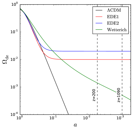
Figure 1: The dark energy density parameter, $\Omega_{\rm de}$, as a function of scale factor, $a$, for the two EDE models studied here, the EDE1 model (red line), EDE2 model (blue line), the Wetterich model (green line) and $\Lambda$CDM (black line). (See Table 1 for the model parameters.) The two black dashed lines indicate, as labelled, redshift 200 when our simulations are started and the CMB redshift, $z\sim$1090.

The dark energy equation of state, $w(z)=P/\rho$, where $P$ is pressure and $\rho$ is density, determines how dark energy influences the expansion of the universe. In the standard $\Lambda$CDM model, the equation of state of the dark energy is a constant, $w_{\Lambda}=-1$, and the dark energy density parameter $\Omega_{\rm de}(z)$ falls rapidly to zero with increasing redshift (see Fig. 1). The cosmological constant can be completely ignored beyond $z\sim 5$, once it accounts for less than $1\%$ of the critical density. However, if the dark energy equation of state is such that $w>-1$, $\Omega_{\rm de}$ will decrease more slowly and the consequences of dark energy will be felt earlier.

Quintessence originates from theoretical models which treat the dark energy as a slowly evolving scalar field. The scalar field can be described by potentials with different properties. Viable models share common features such as reproducing the observed magnitude of the present-day energy density and producing an accelerating expansion at late times. Due to the time-dependent scalar field, the dark energy equation of state evolves. The ratio of the energy density of dark energy to the critical density in quintessence models, $\Omega_{\rm de}$, will be different from that in the $\Lambda$CDM model. This affects the growth of structure (see Fig. 1 for a comparison between $\Omega_{\rm de}$ in $\Lambda$CDM and in the EDE models simulated here; the choice of EDE model is discussed later in § 2.2). Observations constrain the present-day dark energy equation of state to be $w_{0}<-0.8$ (Sánchez et al., 2012). So, EDE models which agree with this constraint should display a transition in $w$ from the present day value ($w\approx-1$) to the early-time value (usually close to zero). How and when this transition happens is the main difference between the various EDE models.

Ideally, the dark energy equation of state should be derived from the potential energy associated with a time dependent scalar field. However, the motivation behind the form of the potential is weak which means that a wide variety of cases have been considered (Corasaniti & Copeland, 2003). One way to carry out a systematic study of the EDE parameter space is to use a parametrization for the dark energy equation of state, $w$, or the dark energy density parameter, $\Omega_{\rm de}$. This approach offers a model-independent and efficient way to investigate the properties of EDE models which display similar behaviour for $w$.

The most commonly used and simplest parametrization to describe the evolution of the equation of state is the two-parameter equation, $w=w_{0}+(1-a)w_{a}$, where $a$ is the expansion parameter (Chevallier & Polarski, 2001; Linder, 2003). However, Bassett, Corasaniti, & Kunz (2004) have shown that a two-parameter equation is not sufficiently accurate to describe the equation of state of the scalar field to better than 5 per cent beyond $z\sim 1$. This problem is even worse when if a two-parameter model is to be used in an N-body simulation which might start at a very high redshift (e.g. $z\approx 100$). More complex parametrizations with more parameters have been proposed which can capture the behaviour seen in a wide range of quintessence models (Corasaniti & Copeland, 2003). However, the additional parameters are hard to constrain in practice given current observations.

Instead we investigate empirical parametrizations of EDE which have three parameters. One was introduced by Wetterich (2004) and is given in terms of the equation of state parameter,

$$w(a)=-\frac{w_{0}}{(1-b\ln(a))^{2}},$$ (1)

where

$$b=-\frac{3w_{0}}{\ln\left(\frac{1-\Omega_{\rm de,e}}{\Omega_{\rm de,e}}\right)+\ln\left(\frac{1-\Omega_{\rm m,0}}{\Omega_{\rm m,0}}\right)}.$$ (2)

Here $w_{0}$ is the dark energy equation of state today, $\Omega_{m,0}$ is the matter (i.e. baryons and cold dark matter) density parameter at $z=0$. $\Omega_{\rm de,0}$ and $\Omega_{\rm de,e}$ are, respectively, the dark energy density parameters today and as $z\to\infty$.

The other empirical parametrization we consider was proposed by Doran & Robbers (2006) and is written in terms of the time evolution of the dark energy density parameter

$$\Omega_{\rm de}(a)=\frac{\Omega_{\rm de,0}-\Omega_{\rm de,e}(1-a^{-3w_{0}})}{\Omega_{\rm de,0}+\Omega_{\rm m,0}a^{3w_{0}}}+\Omega_{\rm de,e}(1-a^{-3w_{0}}).$$ (3)

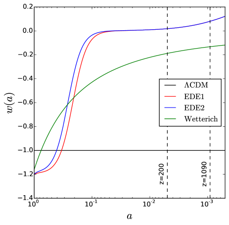
Figure 2: The dark energy equation of state, $w$, as a function of the scale factor, $a$, for the EDE1 model (red line), EDE2 model (blue line), a Wetterich model (green line) and $\Lambda$CDM (black line). (See Table 1.) The two black dashed lines indicate the redshift when the simulations are started ($z=200$) and the CMB redshift ($z\sim 1090$).

Both parametrizations mimic $\Lambda$CDM at low redshift and can provide non-negligible amounts of EDE at early times, depending upon the parameter values adopted. The Doran & Robbers parametrization allows rapid transitions in the dark energy equation of state. The variation of $w(a)$ in the Wetterich parametrization is more gradual as shown in Fig. 2. If we assume $\Omega_{\rm m}+\Omega_{\rm de}=1$ at $z=0$, the two parametrizations yield $\Lambda$CDM, $w(a)=w_{0}=-1$, in the limit when $\Omega_{\rm de,e}=0$.

2.2 Parameter fitting

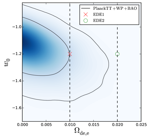
Figure 3: The 2D marginalized distribution in the present day equation of state parameter, $w_{0}$, and the critical density in dark energy at early times, $\Omega_{\rm de}$, using the Doran & Robbers EDE parametrization for the Planck TT, WMAP polarization and BAO data combination. The constraint is compatible with $\Lambda$CDM. The solid black lines show the 68% and 95% confidence intervals. The red cross and green circle indicate, respectively, the EDE1 and EDE2 models which are used in our simulations. The black dashed lines indicate the values of $\Omega_{\rm de}$ in these models.

Changing the equation of state, $w$, from a constant to being time-dependent will affect the evolution of the Universe. The cosmological distance-redshift relation also changes. Cosmological constraints derived for $\Lambda$CDM will not necessarily apply in an EDE universe. We need to re-fit the cosmological parameters for an EDE cosmology and use the best-fitting values in a simulation of such a model rather those derived for $\Lambda$CDM. Here we use observations of the CMB and BAO to find the best-fitting cosmological parameters for EDE models. Using the CMB and BAO data in this way not only allows us to determine the cosmological parameters we should use in simulations, but is also a preliminary test of the viability of EDE parametrization.

To derive the constraints on EDE parameters, we use the CMB measurement from the Planck 2013 data release (Planck Collaboration et al., 2014), which contains the Planck temperature angular power spectrum (TT) and WMAP9 polarization data (WP), in the form of likelihood software. We adapted the Markov Chain Monte-Carlo code, CosmoMC, to work for EDE cosmologies (Lewis & Bridle, 2002a). Some studies, such as Wang & Mukherjee (2006), use CMB distance priors which condense the full temperature fluctuation power spectrum into three quantities which depend on an assumed cosmological model to describe the peak positions and peak height ratios (Komatsu et al., 2009; Wang & Wang, 2013). Although this method is faster, we do not use it here because it results in weaker constraints than using the full data set.

We also use the BAO feature in the galaxy distribution which depends on the horizon scale at matter-radiation decoupling and angular diameter distance to a given redshift. The BAO measurements used are the $z=0.106$ result from the 6dF Galaxy Survey (6dFGS, Beutler et al., 2011), the $z=0.35$ measurement from Sloan Digital Sky Survey Data Release 7 (SDSS DR7, Percival et al., 2010) and the $z=0.57$ measurement from the Baryon Oscillation Spectroscopic Survey (BOSS, Sánchez et al., 2012).

Fig. 3 shows the 2D marginalized distribution for $w_{0}$ and $\Omega_{\rm de,e}$ using the Doran & Robbers parametrization of EDE. $\Lambda$CDM ($w_{0}=-1$,$\Omega_{\rm de,e}=0$) is within the 68% confidence level. The Doran & Robbers cosmologies with 1 and 2 percent EDE are respectively roughly 1 and 2 $\sigma$ away from the best-fitting value. In order to maximize the effects of EDE, here, we choose $w_{0}=-1.2$ and $\Omega_{\rm de,e}=0.01$ as the “EDE1” model, $\Omega_{\rm de,e}=0.02$ as the “EDE2” model rather than using the best fitting values and keep the other cosmological parameters the same between the two models. The EDE1 and EDE2 models are therefore somewhat in tension with the current observational constraints but are formally consistent with the data.

Table 1 summarizes the constraints for the $\Lambda$CDM and EDE cosmologies, assuming a flat universe. In the EDE models, the cosmological parameters show small departures from the best fitting $\Lambda$CDM values. The best fitting result obtained using the Wetterich parametrization gives a negligible amount of EDE, $\Omega_{\rm de,e}\sim 0$, corresponding to $\Lambda$CDM if we fix $w_{0}=-1$. The Wetterich parametrization does not yield any EDE when constrained using current observations. The Doran & Robbers parametrization can reproduce the step-like transition in the dark energy equation of state that results from solving the equations of motion for an EDE potential, so we focus on this parametrization from hereon.

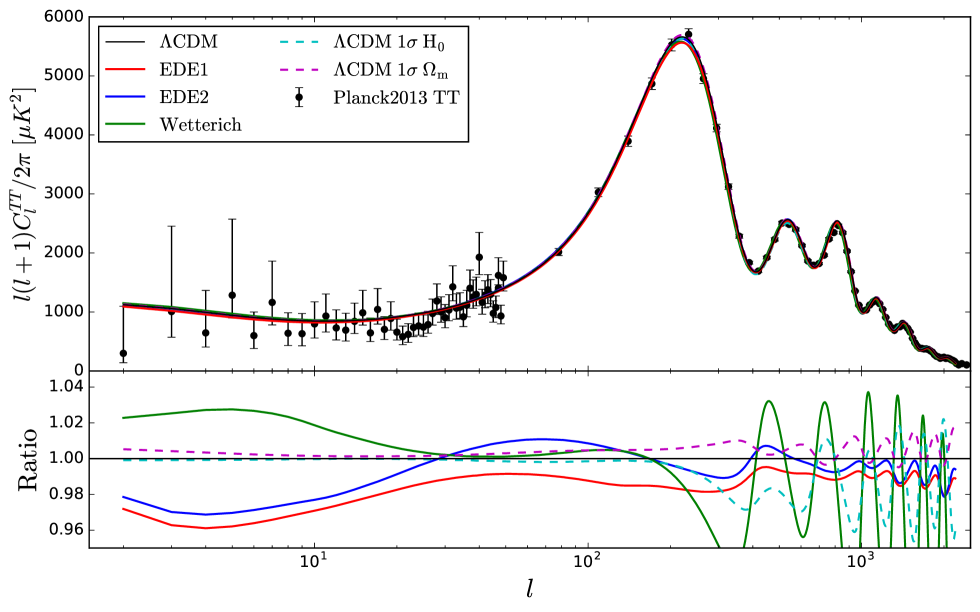
Figure 4: The upper panel shows the cosmic microwave background temperature fluctuation spectra of the EDE1, EDE2, $\Lambda$CDM and Wetterich models from Table 1 compared with the Planck 2013 data (Planck Collaboration et al., 2014) (see legend). Two variants of the $\Lambda$CDM model are also shown, which depart from the best fitting model by similar amounts to the EDE models. The lower panel shows the ratio of these models to $\Lambda$CDM.

Table 1: Summary of the best fitting values using CMB and BAO data for the dark energy parametrizations of Doran & Robbers (labelled EDE1 and EDE2) and Wetterich, along with $\Lambda$CDM. All models have $\sigma_{8}=0.8$.

Parameter	$\Lambda$CDM	EDE1	EDE2	Wetterich
$H_{0}$	67.7	71.9	71.9	70.7
$\Omega_{de}$	0.687	0.719	0.719	0.716
$\Omega_{b}$	0.0488	0.0424	0.0424	0.044
$w_{0}$	-1	-1.2	-1.2	-1.16
$\Omega_{de,e}$	-	0.01	0.02	$<10^{-7}$

Fig. 2 shows the dark energy equation of state as a function of scale factor for the EDE1 and EDE2 models, along with the $\Lambda$CDM model. The corresponding dark energy density parameter as a function of scale factor is shown in Fig. 1. Here, we plot the Wetterich model with $\Omega_{\rm de,e}=10^{-5}$, which is much larger than the value listed in Table 1, but retain the other best-fitting cosmological parameters for comparison. At late times the EDE1 and EDE2 models show very similar behaviour to $\Lambda$CDM, with a rapid transition to $w\approx 0$ at early times. The dark energy parameter remains nearly constant at early times ($z\gtrsim 9$). Even for the tiny amount of EDE considered, the Wetterich model deviates from $\Lambda$CDM from very low redshift. The BAO data probe low redshifts which is why the observational constraints do not allow Wetterich model to have non-negligible EDE.

Since the EDE1 and EDE2 models are not best-fitting models, in order evaluate the effect of the deviations before running simulations, we look at two variant $\Lambda$CDM models for comparison. One is a $\Lambda$CDM model with a value of $\Omega_{\rm m}$ which deviates by $1\sigma$ from the best-fitting value, labelled “$\Lambda$CDM $1\sigma\ \Omega_{\rm m}$”. The other one is a $\Lambda$CDM model with $H_{0}$ deviating by $1\sigma$ from the best-fitting value, named “$\Lambda$CDM $1\sigma\ H_{0}$”. We use the CAMB code (Lewis & Bridle, 2002b) to generate the CMB temperature spectra for those models. Fig. 4 shows the comparison between all the models and the Planck CMB data. It is clear that the CMB peaks of the Wetterich model are shifted to lower multipoles compared to $\Lambda$CDM. All the other models have similar CMB spectra and fit the Planck data reasonably well. At very low multipoles, $l<50$, the “$\Lambda$CDM $1\sigma\ \Omega_{\rm m}$” and “$\Lambda$CDM $1\sigma\ H_{0}$” models are almost the same as $\Lambda$CDM. However, the two Doran & Robbers models deviate from $\Lambda$CDM by up to 4 percent at these multipoles. Hence the differences between the EDE1 and EDE2 models and $\Lambda$CDM are not due to the fact that the EDE models are not formally the best fitting models but rather arise because of the different expansion histories. Fig. 4 also shows that the acoustic oscillations appear at slightly different $l$ in EDE1 and EDE2 than in $\Lambda$CDM, as shown by the oscillations in the ratio of power spectra shown in the lower panel.

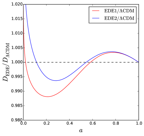
Figure 5: The ratio of the linear growth factor in the EDE models considered here compared to $\Lambda$CDM as labelled. The linear growth factor is normalized to unity at $z=0$ in all models.

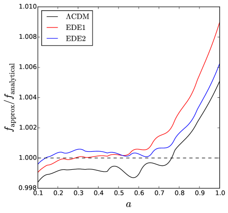
Figure 6: A comparison of growth rate obtained using an approximation, $f_{\rm approx}$, estimated from Eqn. 7 and the analytical value, $f_{\rm analytical}$ calculated using Eqn. 5 in the EDE and $\Lambda$CDM models as labelled.

2.3 Linear growth rate

The evolution of linear growth rate reflects the different growth histories of structure between the EDE and $\Lambda$CDM cosmologies. If we assume the dark matter perturbations are small, i.e., the density contrast $\ll 1$, the power spectrum, $P(k,t)$ can be written as a function of time,

$$P(k,t)=\frac{D(t)^{2}}{D(t_{0})^{2}}P(k,t_{0}).$$ (4)

Here, $D(t_{0})$ is the linear growth factor today and is obtained by solving the differential equation (Linder, 1998):

$$D^{\prime\prime}+\frac{2}{3}\left(1-\frac{w(a)}{1+X(a)}\right)\frac{D^{\prime}}{a}-\frac{3}{2}\frac{X(a)}{1+X(a)}\frac{D}{a^{2}}=0,$$ (5)

where

$$X(a)=\frac{\Omega_{\rm m}}{1-\Omega_{\rm m}}e^{-3\int_{a}^{1}d\ln a^{\prime}w(a^{\prime})}.$$ (6)

The linear growth rate is defined as $f=d\ln D/d\ln a$. Fig. 5 shows the ratio of the linear growth factor in the EDE1 and EDE2 models to that in $\Lambda$CDM. Before $z=10$, the growth factor is enhanced by a few percent in the EDE1 and EDE2 compared with $\Lambda$CDM, before showing a reduction for $z\sim 2$–$10$.

Although it is straightforward to obtain the linear growth factor by solving Eqn. 5, some parametrizations of linear growth rate have become popular. Peebles (1976) proposed a widely used parametrization, $f(z)\approx\Omega_{m}^{\gamma}$, where $\gamma=0.6$ is the growth index. Linder (2005) suggested the more accurate form

$$\gamma=0.55+0.05[1+w(z=1)],$$ (7)

which gives $f=\Omega_{m}^{0.55}$ for a $\Lambda$CDM cosmology.

In order test the accuracy of the Linder parametrization for the growth factor, we plot in Fig 6 the approximate growth rate, $f_{\rm approx}$, given by Eqn. 7 divided by the value $f_{\rm analytical}$ calculated from Eqn. 5. For the EDE1 and EDE2 models and $\Lambda$CDM, the approximation reproduces the linear growth rate to better than 1% over the redshift range from $z=0$ up to $z=10$. Nevertheless, at late times the inaccuracy in the growth rate obtained from Eqn. 7 is comparable to the magnitude of the departure from the $\Lambda$CDM growth rate, which means that the full calculation should be used.

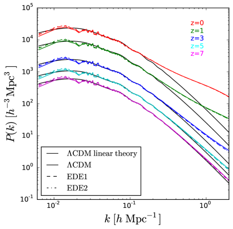
Figure 7: The matter power spectra measured in the EDE1, EDE2 and $\Lambda$CDM simulations. Different line styles refer to the results for different models and different colours show the measurements at different redshifts, as indicated by the key. The smooth black curves show the predictions of linear perturbation theory in $\Lambda$CDM. Differences between the EDE1 and EDE2 models and the $\Lambda$CDM results are apparent at very small and high wavenumbers.

2.4 N-body Simulations

We have carried out three large volume, moderate resolution N-body simulations for $\Lambda$CDM and the EDE1 and EDE2 cosmologies, using a memory-efficient version of the TreePM code GADGET-2(Springel, 2005), called L-GADGET2. The code was used in Jennings et al. (2010) and has been modified in order to allow a time dependent equation of state for dark energy. We assume a flat universe and use the cosmological parameters in Table 1. The simulations use grid initial conditions with $N=2048^{3}$ dark matter particles in a computational box of a comoving length of $1500\ h^{-1}{\rm Mpc}$. The particle mass is $3.413\times 10^{10}h^{-1}M_{\odot}$ for $\Lambda$CDM and $3.064\times 10^{10}h^{-1}M_{\odot}$ for the EDE1 and EDE2 models. The initial mean inter-particle separation is $0.732\ h^{-1}{\rm Mpc}$. We adopt a comoving softening length of $\epsilon=15\ h^{-1}\rm kpc$. The initial conditions were generated using the L-GENIC code (Springel et al., 2005), which has also been adapted to handle a time variable equation of state. A self-consistent linear theory power spectrum for each model is generated using CAMB (Lewis & Bridle, 2002b). The normalisation extrapolated to $z=0$ is $\sigma_{8}=0.8$ for all simulations. The starting redshift is $z=199$. We have tested that the results presented have converged for these choices of particle number, softening length and starting redshift. Here we are interested in large-scale structure, redshift space distortions and rare objects, which is why we chose a large simulation box.

3 Results

Here we present a range of results from our N-body simulations: the matter power spectrum in real and redshift space (§ 3.1), the dark matter halo mass function (§ 3.2), and the distribution of counts-in-cells (§ 3.3).

3.1 Matter power spectrum

The power spectrum of fluctuations in the matter distribution is a key statistic that encodes information about the cosmological parameters and is the starting point for determining many quantities, such as the clustering of galaxies and the weak gravitational lensing of faint galaxies. The presence of dark energy at early times in the EDE cosmologies can change the form of the matter power spectrum compared to that in $\Lambda$CDM and may allow us to distinguish between models. The use of N-body simulations allows this comparison to be extended into the nonlinear regime.

3.1.1 The power spectrum in real space

Fig. 7 shows the matter power spectra at redshifts $z=0,1,3,5,7$ measured from the $\Lambda$CDM, EDE1 and EDE2 simulations, together with the linear perturbation theory power spectra for $\Lambda$CDM. At $z=0$, the power spectra have very similar amplitudes at intermediate wavenumbers because the three models have been normalized to have the same value of $\sigma_{8}$ today ($\sigma_{8}=0.8$). The power spectra, however, are noticeably different at very small wavenumbers (large scales). There are also small differences apparent deep into the nonlinear regime at high wavenumbers (small scales).

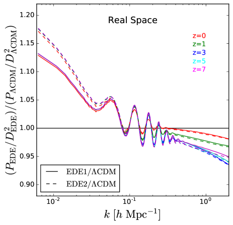
Figure 8: The ratio of matter power spectra measured in real space in the EDE1 and EDE2 simulations to those in $\Lambda$CDM. This ratio is plotted after taking into account differences in the linear growth factor at a fixed redshift between the models. The differences on large scales (small $k$) show that it is important to use a linear theory power spectrum in the simulations that is consistent with the expansion history and cosmological parameters in the EDE models.

The EDE models differ from $\Lambda$CDM on large scales at all plotted redshifts. This is due to the difference in the expansion histories in these models compared with that in $\Lambda$CDM. This changes the rate at which fluctuations grow, particularly around the transition from radiation to matter domination, which alters the shape of the turnover in the power spectrum (Jennings et al., 2010). To drill down further into the comparison between the power spectra in the models we now compare the simulation measurements after taking into account differences in the linear growth factor at a given redshift (as plotted in Fig. 5). Fig. 8 shows the ratio of matter power spectrum after dividing by the linear growth factor squared, $D(a)^{2}$, for each model. The EDE1 and EDE2 models differ from $\Lambda$CDM by up to 13% and 17% on large scales repectively, with the ratio showing a slight dependence on redshift. But the differences between the models on small scales (high $k$) are more modest, reaching at most around 5%. Using the linear growth factor in this way helps to isolate the impact of the different expansion histories in the models (see Jennings et al. 2010 for a more extended discussion of this comparison). When plotted in this way, the ratios of power spectra measured at different redshifts coincide. The residual differences at high wavenumbers are due to the different growth histories in the models.

The non-negligible difference in Fig. 8 illustrates the need to use a consistent linear theory power spectrum to generate the initial conditions in the N-body simulation rather than using a $\Lambda$CDM spectrum in all cases.

The conclusion of this subsection is that it should be possible to distinguish an EDE model from $\Lambda$CDM using the shape of power spectrum on large scales, well into the linear perturbation theory regime. The bulk of observational measurements of the power spectrum probe the clustering in ”redshift” space, so next we extend the comparison to include the contribution from gravitationally induced peculiar velocities.

3.1.2 The power spectrum in redshift space

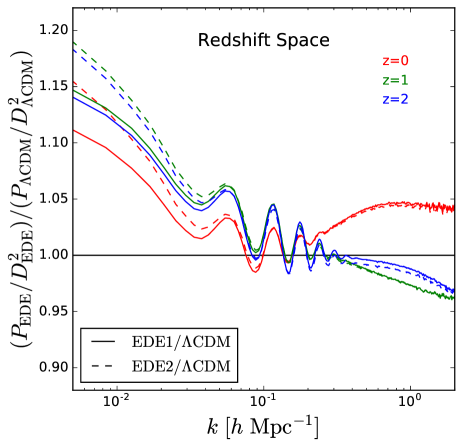
Figure 9: The ratio of redshift space power spectra measured in the EDE1 and EDE2 simulations after dividing by the square of the linear growth factor in each model at the redshift in question to that in $\Lambda$CDM as labelled (note that the range of redshifts compared in this plot is smaller than in Fig. 8).

We model clustering in redshift space using the distant observer approximation. We adopt one axis as the line of sight direction and displace the particles along this axis according to the component of their gravitationally induced peculiar velocity in this direction. Even though we use a large simulation volume, there is still appreciable scatter in the clustering when viewed in redshift space, so we repeat this procedure for each axis in turn and average the results to obtain our estimate of the matter power spectrum in redshift space.

Fig. 9 shows the ratio of the redshift space power spectra measured in the simulations after removing differences in the linear growth factors of the Doran & Robbers cosmologies to that in $\Lambda$CDM. On large scales, the EDE power spectra are 10% - 20% higher in amplitude than the $\Lambda$CDM power spectrum, which is similar to the result found in real space. On small scales, due to the nonlinear effects, there are clear differences in the $P(k)$, but these are smaller than 5 per cent. However, unlike the case of the real space power spectra, dividing by growth factor squared does not reduce the differences between the ratios measured at different redshifts. Instead, the difference between the rations measured between the redshift space power spectra in a given pair of models increases slightly on large scales. This is because the linear growth factor does not account for all of the linear theory differences between the power spectra in redshift space.

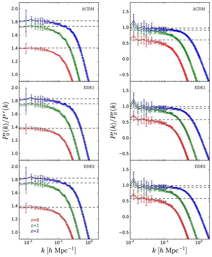
Figure 10: The distortion of clustering due to peculiar velocities. Left panel: the ratio of the monopole redshift power spectra to real space power spectra measured from the N-body simulations at $z=0,1$ and $2$. Different colours show the results for different redshifts as labelled. The dashed lines show the linear theory prediction. Right panel: the ratio of the quadrupole to monopole moments of the redshift power spectra measured from the simulations. Each panel shows the result for a different model as labeled. For comparison, the $\Lambda$CDM measurements are reproduced as grey lines in the EDE1 and EDE2 panels

To further investigate the contributions of the velocity dispersion and nonlinearities to the form of the redshift space power spectrum, we compare the ratio of the spherically averaged power spectra in redshift space and real space in left column of Fig. 10. The linear theory prediction, known as the “Kaiser formula” given by $P^{s}(k,\mu)=P^{r}(k)(1+\mu^{2}\beta)^{2}$, is plotted as black dashed lines in Fig. 10. Here $P_{r}(k)$ is the power spectrum in real-space, $\mu$ is the cosine of the angle between the line of sight and the peculiar motion of the dark matter particle and $\beta=f$ for the dark matter. The linear theory monopole ratio depends on redshift through the value of the matter density parameter. The value of linear growth rate is calculated using the parametrization $f(z)=\Omega^{\gamma}$, where $\gamma$ is given by Eqn. 7. The error bars illustrate the scatter in $P^{s}(k)$ obtained by using the x, y, z directions in turn as the line-of-sight direction. At $z=0$, the left panel of Fig. 10 shows that the Kaiser formula only fits the simulation results on very large scales, $k<0.03h\rm{Mpc^{-1}}$, as reported by Jennings et al. (2011). The departure from the linear theory prediction is due to a combination of nonlinearities and the damping effects of peculiar velocities, even though this is often modelled as arising solely due to damping. Nonlinear effects are important for $k>0.03h\rm{Mpc^{-1}}$ even though the linear regime is typically believed to hold out to $k\sim 0.1$ – $0.25h\rm{Mpc^{-1}}$. The Kaiser prediction agrees with the simulation results over a slightly wider range of scales at higher redshifts because the nonlinear effects are smaller than they are that at $z=0$. In the right panel of Fig. 10 we plot the ratio of the quadpole to monopole moments of the redshift space power spectrum, $P^{s}_{2}(k)/P^{s}_{0}(k)$, for each cosmology at $z=0$, $1$ and $2$. The Kaiser limit agrees with the simulation results for $k<0.05h\rm{Mpc^{-1}}$ at $z=0$ which is a slightly higher wavenumber than was the case for the monopole ratio. The departures from the redshift space distortions expected in $\Lambda$CDM (shown by the grey lines in Fig. 10) are small, and well within our estimated errors.

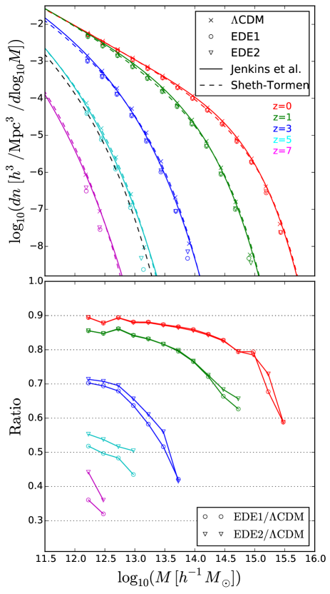
Figure 11: The mass function of dark matter halos measured from the simulations. The upper panel shows the halo mass functions at different redshifts. The crosses show $\Lambda$CDM, circles EDE1 and triangles EDE2. The solid and dashed lines show the Jenkins et al. and Sheth-Tormen mass functions respectively for $\Lambda$CDM. The lower panel shows the ratio of dark matter halo mass functions in the EDE1 and EDE2 cosmologies to that measured in $\Lambda$CDM.

3.2 Halo mass function

The mass function of dark matter halos, defined as the number of halos per unit volume with masses in the range $M$ to $M+dM$, $n(M,z)$, is an important characteristic of the dark matter density field which is affected by the expansion rate of the Universe.

We use the friends-of-friends (FOF) algorithm (Davis et al., 1985) which is built into the L-GADGET2 code to identify dark matter halos, using a linking length of $b=0.2$ times the mean inter-particle separation. We retain FOF groups down to 20 particles. In Fig. 11 we plot the halo mass functions measured from the $\Lambda$CDM, EDE1 and EDE2 simulations at $z=0,1,3,7$. For comparison we also plot the Jenkins et al. (2001) and Sheth & Tormen (1999) mass functions evaluated for $\Lambda$CDM. The lower panel of Fig. 11 shows the ratio of the mass functions measured in the EDE cosmologies to that in $\Lambda$CDM. The differences in the mass functions at low redshift ($z\leq 1$) are small, in agreement with results of Francis, Lewis, & Linder (2009). The EDE mass functions agree with $\Lambda$CDM to within 20% for halos with masses around $10^{12.0}$–$10^{13.5}h^{-1}M_{\odot}$ at $z=1$.

The difference between the halo mass functions in EDE and $\Lambda$CDM increases with increasing redshift. This is due in part to the difference in the linear growth factors getting larger between the EDE and $\Lambda$CDM cosmologies going back in time from the present day. Also, because the simulations have a fixed mass resolution, the results probe rarer halos with increasing redshift. The abundance of these objects is sensitive to the matter power spectrum at smaller wavenumbers, where we found the largest differences between EDE and $\Lambda$CDM. At $z=7$, $\Lambda$CDM predicts 2.5 times as many halos as are found in the EDE cosmologies.

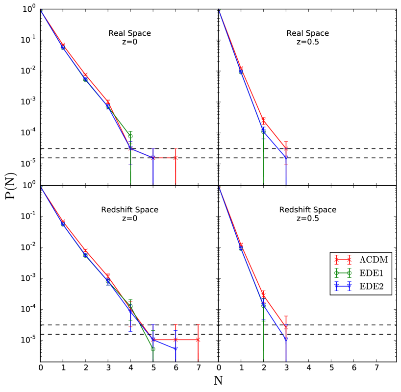
Figure 12: The counts in cells distribution for extreme structures. The probability distribution of finding a given number of halos with mass larger than $5\times 10^{14}\ h^{-1}\rm M_{\odot}$ in cubic cells of side $37.5\ h^{-1}\rm Mpc$. The x-axis is the number of halos in the cell. In the upper panels, the cell counts are measured in the real space, while in the lower panels the counts are measured in redshift space. The two dashed horizontal lines in each panel indicate the probability to find one cell and two cells in the whole simulation box.

This prediction could be tested by using a proxy for the halo mass function at high redshift, such as the galaxy luminosity function (Jose et al. (2011) proposed a similar test to probe the mass of neutrinos). To make the connection to the observable Universe, a model is needed to connect the mass of a dark matter halo to the properties of the galaxy it hosts. We have evaluated this approach by carrying out an abundance matching exercise between the halo mass functions and the observed luminosity function of galaxies in the rest-frame ultra-violet. This simple procedure assigns one galaxy to each dark matter halo, ignoring any contribution from satellite galaxies. The translation between halo mass and galaxy luminosity can be described by a mass-to-light ratio. Despite the large differences in the halo mass functions between cosmologies, the differences in the implied mass-to-light ratios are quite modest and well within the current uncertainties in our knowledge of the galaxy formation process. Hence, we conclude that any of these cosmologies could be made to match the observed galaxy luminosity function at high redshift with plausible mass to light ratios, and that it would be difficult to use the galaxy luminosity function to distinguish between the models.

3.3 Extreme structures

We have seen in Section 3.1 that the power spectra of the $\Lambda$CDM and EDE energy models are similar on small scales, particularly once the differences between the expansion histories in the models have been taken into account. The power spectrum is a second moment of the density field and so does not probe the tails of the distribution of density fluctuations, which could carry the imprint of differences in the growth history of fluctuations.

Fluctuations in the density field can be quantified by measuring the distribution of fluctuations smoothed over cells, commonly referred to as counts-in-cells. Rather than formally measuring the higher order moments of the counts-in-cells distribution, which rapidly becomes infeasible even with simulations of the volume used here, we instead compare the high fluctuation tails of the distributions directly in different cosmologies.

Following Yaryura, Baugh, & Angulo (2011), in order to connect more closely with observables rather than looking at fluctuations in the overall matter distribution, we consider the counts-in-cells of cluster-mass dark matter halos. In particular, we look for “hot” cells that contain a substantial number of massive halos. The choice of halo mass and the definition of hot cells is motivated by results from the two-degree field galaxy redshift survey (2dFGRS). Croton et al. (2004) identified two hot cells in the 2dFGRS. Padilla et al. (2004) found 10 groups with an estimated mass over $5\times 10^{14}\ h^{-1}\rm M_{\odot}$ in each cell, by cross matching the hot cells in the galaxy distribution with the 2dFGRS Percolation Inferred Galaxy Group catalogue (2PIGG catalogue, Eke et al., 2004).

Here we use a cubical cell of side $37.5\ h^{-1}\rm Mpc$, which corresponds to a slightly smaller volume than the equivalent size of the spherical cell used by Croton et al. (2004). We then count the number of dark matter halos with $M_{\rm halo}>5\times 10^{14}\ h^{-1}\rm M_{\odot}$ inside each cell. We use the jackknife method to estimate the errors on the distribution of counts (Shao, 1986; Norberg et al., 2009) . Put simply, the jackknife is a resampling technique which works by systematically leaving out each subset of data in turn from a whole dataset to generate “new” subsamples. Here a subset is defined to be a volume within the simulation. Then, the overall jackknife estimate of $\delta$ can be found by averaging over all the subsamples, given by

$$\delta_{\rm Jack}=\frac{1}{N}\sum_{i=1}^{N}\delta_{i},$$ (8)

where $N$ is the number of subsamples. The jackknife error is calculated as

$$\sigma_{\rm Jack}=\sqrt{(N-1)\sum_{i=1}^{N}\frac{(\delta_{i}-\delta_{\rm Jack})^{2}}{N}}.$$ (9)

We use 64 spatial subsamples in our analysis, dividing each side of simulation box equally into four parts.

Fig. 12 shows the distribution of cell counts for the three cosmologies in both real space and redshift space at $z=0$ and $0.5$. The $x$-axis gives the number of halos per cell above the specified mass limit. The $y$-axis is the normalized probability to find such a cell. In redshift space, we also considered the scatter from using the three axes in turn as the line-of-sight. The high cell count tails are very similar, but $\Lambda$CDM consistently predicts more “hot” cells. The “hottest” cells only contain 7 halos in $\Lambda$CDM at $z=0$, which is lower than suggested by the 2dFGRS superclusters. This could be because the FOF halo mass, which we used to select the halos, does not match the halo mass estimated from the galaxy group catalog. Yaryura, Baugh, & Angulo (2011) showed that by perturbing the FOF halo mass by the systematic bias and scatter expected in the masses returned by a group finder run on a galaxy catalogue, the number of hot cells increases.

Again, the differences between the predicted count distributions are smaller than the estimated errors on the measurement and so could only be probed by a survey covering a volume that is much larger than our simulations.

4 Conclusions

One of the main science goals of future wide field galaxy surveys is to distinguish a cosmological constant from other scenarios for the acceleration of the cosmic expansion, such as dynamical dark energy models. Here we have examined a particular class of dynamical dark energy model which display a small but non-negligible amount of dark energy at early times, which are referred to as early dark energy models. Such models could be motivated by a choice of potential for the scalar field describing the dark energy. Instead, to confront these models with the currently available cosmological constraints in an efficient way, we chose to use a simple description in which the density parameter of the dark energy is parametrized as a function of the expansion factor, the present day values of the dark energy and matter density parameters, the present equation of state parameter of the dark energy and the asymptotic value of the density parameter of dark energy at early times. Once constrained, the model can be described by the resulting time dependence of the equation of state parameter.

The step of constraining the early dark energy model to reproduce current observations is a critical one. In fact, the best fitting models, even with the observational constraints available today favour models without any dark energy at early times, a conclusion that has already been reached by other studies (Planck Collaboration et al., 2014). Nevertheless, within the range of models that remain compatible with current data, it is possible to find examples with interesting amounts of early dark energy. Increasing the amount of early dark energy in the model tends to favour a more negative equation of state parameter at the present day than the canonical $w=-1$ which corresponds to the cosmological constant. We have investigated two models which, whilst not best fitting models, are still compatible with the observations at the $1-\sigma$ (EDE1 with 1% of the critical density in dark energy at early times) and $2-\sigma$ levels (EDE2 with 2% of the critical density in dark energy at early times); both models have $w_{0}=-1.2$.

Previous simulation work on early dark energy models suggested that a clear signature that could be testable against $\Lambda$CDM is the halo mass function (Francis, Lewis, & Linder, 2009; Grossi & Springel, 2009). In a simple picture, the presence of a small but unignorable amount of dark energy at early epochs increases the rate at which the universe expands, making it harder for structure to form. If the models are set up to have the same value of $\sigma_{8}$ today, this means that structure has to form at a smaller expansion factor or earlier time in the early dark energy model. Hence, a larger number density of massive haloes is predicted in early dark energy models compared to $\Lambda$CDM.

Our results show that this simple picture of early structure formation with early dark matter is not a generic feature of these models. After constraining the models against current observations, we find that the evolution of the linear growth rate of fluctuations in the early dark energy models is remarkably close to that in $\Lambda$CDM. At the earliest epochs, the EDE2 growth rate exceeds that in $\Lambda$CDM by just $2\%$ before lagging behind until catching up around $z\sim 0.8$ and then exceeding the $\Lambda$CDM growth rate by less than $0.5\%$.

The dark matter halo mass function in the early dark energy simulations shows fewer massive haloes than we find in the $\Lambda$CDM simulation. This difference in the halo mass function could be tested using the high redshift galaxy luminosity function (as suggested by Jose et al. (2011) to probe the nature of massive neutrinos). The difference in halo abundance is, however, modest, and could be accounted for by our lack of knowledge of the relevant galaxy formation physics. We find a small difference in the abundance of “hot cells” in the distribution of dark matter halos between early dark energy and $\Lambda$CDM, though this will be challenging to measure, requiring huge survey volumes.

The cleanest signature we have found of the presence of dark energy at early times is in the shape of the matter power spectrum. The more rapid expansion rate around the epoch of matter radiation equality in early dark energy models compared to $\Lambda$CDM changes the shape of the turn over in the matter power spectrum (Jennings et al., 2010). This effect is visible in the linear theory power spectrum and is present on scales on which we would expect scale dependent effects in galaxy bias to be small (Angulo et al., 2008). To probe this effect it will necessary to retain the full shape information for the galaxy power spectrum, rather than isolating the scale of the baryonic acoustic oscillation feature (Sánchez, Baugh, & Angulo, 2008). Tentative measurements of the matter power spectrum on the scale of the turnover have already been made by the WiggleZ Dark Energy survey (Poole et al., 2013). Future large-area radio surveys conducted with the SKA pathfinder experiments, MeerKAT and ASKAP have the potential to probe the existence of early dark energy by providing more accurate measurements of the turnover in the power spectrum.

References

- Angulo et al. (2008) Angulo R. E., Baugh C. M., Frenk C. S., Lacey C. G., 2008, MNRAS, 383, 755
- Bassett et al. (2004) Bassett B. A., Corasaniti P. S., Kunz M., 2004, ApJ, 617, L1
- Beutler et al. (2011) Beutler F. et al., 2011, MNRAS, 416, 3017
- Caldwell et al. (1998) Caldwell R. R., Dave R., Steinhardt P. J., 1998, Physical Review Letters, 80, 1582
- Chevallier & Polarski (2001) Chevallier M., Polarski D., 2001, International Journal of Modern Physics D, 10, 213
- Copeland et al. (2006) Copeland E. J., Sami M., Tsujikawa S., 2006, International Journal of Modern Physics D, 15, 1753
- Corasaniti & Copeland (2003) Corasaniti P. S., Copeland E. J., 2003, Phys. Rev. D, 67, 063521
- Croton et al. (2004) Croton D. J. et al., 2004, MNRAS, 352, 1232
- Davis et al. (1985) Davis M., Efstathiou G., Frenk C. S., White S. D. M., 1985, ApJ, 292, 371
- Doran & Robbers (2006) Doran M., Robbers G., 2006, J. Cosmology Astropart. Phys, 6, 26
- Efstathiou et al. (2002) Efstathiou G. et al., 2002, MNRAS, 330, L29
- Eke et al. (2004) Eke V. R. et al., 2004, MNRAS, 348, 866
- Ferreira & Joyce (1998) Ferreira P. G., Joyce M., 1998, Phys. Rev. D, 58, 023503
- Fontanot et al. (2012) Fontanot F., Springel V., Angulo R. E., Henriques B., 2012, MNRAS, 426, 2335
- Francis et al. (2009) Francis M. J., Lewis G. F., Linder E. V., 2009, MNRAS, 394, 605
- Grossi & Springel (2009) Grossi M., Springel V., 2009, MNRAS, 394, 1559
- Halliwell (1987) Halliwell J. J., 1987, Physics Letters B, 185, 341
- Jenkins et al. (2001) Jenkins A., Frenk C. S., White S. D. M., Colberg J. M., Cole S., Evrard A. E., Couchman H. M. P., Yoshida N., 2001, MNRAS, 321, 372
- Jennings et al. (2010) Jennings E., Baugh C. M., Angulo R. E., Pascoli S., 2010, MNRAS, 401, 2181
- Jennings et al. (2011) Jennings E., Baugh C. M., Pascoli S., 2011, MNRAS, 410, 2081
- Jose et al. (2011) Jose C., Samui S., Subramanian K., Srianand R., 2011, Phys. Rev. D, 83, 123518
- Komatsu et al. (2009) Komatsu E. et al., 2009, ApJS, 180, 330
- Lewis & Bridle (2002a) Lewis A., Bridle S., 2002a, Phys. Rev. D, 66, 103511
- Lewis & Bridle (2002b) Lewis A., Bridle S., 2002b, Phys. Rev. D, 66, 103511
- Linder (1998) Linder E. V., 1998, New Scientist, 2127, 45
- Linder (2003) Linder E. V., 2003, Physical Review Letters, 90, 091301
- Linder (2005) Linder E. V., 2005, Phys. Rev. D, 72, 043529
- Norberg et al. (2009) Norberg P., Baugh C. M., Gaztañaga E., Croton D. J., 2009, MNRAS, 396, 19
- Padilla et al. (2004) Padilla N. D. et al., 2004, MNRAS, 352, 211
- Peebles (1976) Peebles P. J. E., 1976, ApJ, 205, 318
- Percival et al. (2010) Percival W. J. et al., 2010, MNRAS, 401, 2148
- Planck Collaboration et al. (2014) Planck Collaboration et al., 2014, A&A, 571, A16
- Planck Collaboration et al. (2015a) Planck Collaboration et al., 2015a, ArXiv e-prints
- Planck Collaboration et al. (2015b) Planck Collaboration et al., 2015b, ArXiv e-prints
- Poole et al. (2013) Poole G. B. et al., 2013, MNRAS, 429, 1902
- Ratra & Peebles (1988) Ratra B., Peebles P. J. E., 1988, Phys. Rev. D, 37, 3406
- Sánchez et al. (2008) Sánchez A. G., Baugh C. M., Angulo R. E., 2008, MNRAS, 390, 1470
- Sánchez et al. (2009) Sánchez A. G., Crocce M., Cabré A., Baugh C. M., Gaztañaga E., 2009, MNRAS, 400, 1643
- Sánchez et al. (2012) Sánchez A. G. et al., 2012, MNRAS, 425, 415
- Shao (1986) Shao J., 1986, The Annals of Statistics, 14, 1322
- Sheth & Tormen (1999) Sheth R. K., Tormen G., 1999, MNRAS, 308, 119
- Springel (2005) Springel V., 2005, MNRAS, 364, 1105
- Springel et al. (2005) Springel V. et al., 2005, Nature, 435, 629
- Steinhardt et al. (1999) Steinhardt P. J., Wang L., Zlatev I., 1999, Phys. Rev. D, 59, 123504
- Wang & Mukherjee (2006) Wang Y., Mukherjee P., 2006, ApJ, 650, 1
- Wang & Wang (2013) Wang Y., Wang S., 2013, Phys. Rev. D, 88, 043522
- Wetterich (1988) Wetterich C., 1988, Nuclear Physics B, 302, 645
- Wetterich (1995) Wetterich C., 1995, A&A, 301, 321
- Wetterich (2004) Wetterich C., 2004, Physics Letters B, 594, 17
- Yaryura et al. (2011) Yaryura C. Y., Baugh C. M., Angulo R. E., 2011, MNRAS, 413, 1311