Analysis of mechanisms that could contribute to neutrinoless double-beta decay

Abstract

Neutrinoless double-beta decay is a beyond the Standard Model process that would indicate that neutrinos are Majorana fermions, and the lepton number is not conserved. It could be interesting to use the neutrinoless double-beta decay observations to distinguish between several beyond Standard Model mechanisms that could contribute to this process. Accurate nuclear structure calculations of the nuclear matrix elements necessary to analyze the decay rates could be helpful to narrow down the list of contributing mechanisms. We investigate the information one can get from the angular and energy distribution of the emitted electrons and from the half-lives of several isotopes, assuming that the right-handed currents exist. For the analysis of these distributions, we calculate the necessary nuclear matrix elements using shell model techniques, and we explicitly consider interference terms.

I Introduction

Neutrinoless double-beta decay, if observed, would signal physics beyond the Standard Model (SM) that could be discovered at energies significantly lower than those at which the relevant degrees of freedom could be excited. The black-box theorems Schechter and Valle (1982); Nieves (1984); Takasugi (1984); Hirsch et al. (2006) would indicate that the neutrinos are Majorana fermions, and the lepton number is violated in this process by two units.

However, it could be challenging to further use the neutrinoless double-beta decay observations to distinguish between many beyond Standard Model mechanisms that could contribute to this process Vergados et al. (2012); Horoi (2013). Accurate nuclear structure calculations of the nuclear matrix elements (NME) necessary to analyze the decay rates could be helpful to narrow down the list of contributing mechanisms and to better identify the more exotic properties of the neutrinos, such as the existence of the heavy sterile partners that could interact through right-handed currents Keung and Senjanovic (1983); Barry and Rodejohann (2013); Deppisch et al. (2016). The NME for the standard mass mechanism were thoroughly investigated using several nuclear structure models. Figure 13 of Ref. Neacsu and Horoi (2015) shows some of these NME for isotopes of immediate experimental relevance. Here, we describe the status of the shell model calculations of these NME Horoi (2013); Neacsu and Horoi (2015); Brown et al. (2014); Sen’kov and Horoi (2014); Sen’kov et al. (2014); Sen’kov and Horoi (2013); Horoi and Brown (2013); Neacsu et al. (2012); Horoi and Stoica (2010); Horoi et al. (2007) and their relevance for discriminating possible competing mechanisms that may contribute to the neutrinoless double-beta decay process.

One possible alternative/competing mechanism considers the contribution from the exchange of the heavy, mostly sterile, neutrinos Keung and Senjanovic (1983); Barry and Rodejohann (2013); Deppisch et al. (2016). The exchange of left-handed heavy neutrinos is shown to be negligible in most cases Mitra et al. (2012); Blennow et al. (2010). The exchange of the right-handed heavy neutrinos is predicted by left-right symmetric models Pati and Salam (1974); Mohapatra and Pati (1975); Senjanovic and Mohapatra (1975); Keung and Senjanovic (1983); Barry and Rodejohann (2013), which are presently under active investigation at LHC Khachatryan et al. (2014); Deppisch et al. (2016). In either case, the same heavy neutrino-exchange NME are necessary for the analysis of the data. For example, considering only the competition between the light left-handed neutrino-exchange mechanism and the heavy right-handed neutrino-exchange mechanism, one could identify the dominant effect using half-lives of several isotopes, such as ⁷⁶Ge and ¹³⁶Xe Faessler et al. (2011). Some of these heavy neutrino-exchange NME for isotopes of immediate experimental relevance are shown in Fig. 14 of Ref. Neacsu and Horoi (2015). The range of these matrix elements is quite large due to their sensibility to the short-range correlation effects that were not treated consistently. One important improvement of these calculations would be obtaining an effective transition operator that takes into account consistently the short-range correlation effects and the effects of the missing single particle orbits from the model space Holt and Engel (2013).

Some other low-energy effects of the left-right symmetric models, such as those due to the so called $\lambda$ and $\eta$ mechanisms Doi et al. (1985); Barry and Rodejohann (2013), could be identified experimentally if one could measure the angular and the energy distribution of the emitted electrons Arnold and et al (2010), but the analysis requires knowledge of additional NME that one can calculate. Finally, some more exotic possibilities Vergados et al. (2012); Prezeau et al. (2003) leading to one- and two-pion exchange NME Gehman and Elliott (2007) were also calculated in the past within the interacting shell model approach Horoi (2013); Horoi and Brown (2013), and quasiparticle random phase approximation (QRPA) (see, e.g., Ref. Vergados et al. (2012) and references therein). A more general approach that includes a complete set of dimension six and dimension nine operators to the SM Lagrangian, as well as R-parity violating SUSY contributions, Kaluza-Klein modes in higher dimensions Bhattacharyya et al. (2003); Deppisch and Päs (2007), violation of Lorentz invariance and equivalence principle Leung (2000); Klapdor–Kleingrothaus et al. (1999); Barenboim et al. (2002), is given in Refs. Pas et al. (1999); Deppisch et al. (2012). Information from double-beta decay can help constrain these contributions, but additional information from the colliders is needed for a full analysis.

In this paper, we consider the possibility of disentangling the contributions of the right-handed currents to the neutrinoless double-beta decay process. Our analysis mostly focuses on the information one can get from the two-electron energy and angular distributions, which could be used to distinguish contributions coming from the $\lambda$ and $\eta$ mechanisms from those of the usual light neutrino-exchange mechanism. The analysis is done for ⁸²Se, which was chosen as a baseline isotope by the SuperNEMO experiment Arnold and et al (2010); Bongrand (2015). During the preparation of this manuscript, we also found a more general analysis of the terms contributing to the angular and energy distributions for most of the double-beta decay isotopes based on improved phase space factors and QRPA NME Stefanik et al. (2015). Efforts of separating these effects are not new (see, e.g., Refs. Doi et al. (1983); Tomoda et al. (1986); Hirsch et al. (1994); Simkovic et al. (2001); Bilenky and Petcov (2004) among others). Our analysis is however more detailed and more specific to the decay of the ⁸²Se isotope. It considers the competitions between the mass mechanisms and the heavy right-handed neutrino-exchange mechanism if the contributions from $\lambda$ and $\eta$ mechanisms are ruled out by the two-electron angular and energy distributions.

The paper is organized as follows: Section II presents the general formalism used to describe the neutrinoless double-beta decay under the assumption that the right-handed currents would contribute. Section III describes the associated two-electron angular and energy distributions. Section IV analyzes the two-electron angular and energy distributions for different scenarios that consider different relative magnitudes of the $\lambda$ and $\eta$ mechanism amplitudes (please notice the changes of notation). Section V considers the possibility of disentangling the mass mechanisms from the heavy right-handed neutrino-exchange mechanism, if the $\lambda$ and $\eta$ contributions could be ruled out by the two-electron energy and angular distributions. Section VI is devoted to conclusions, and Appendixes A, B, and C present detailed formulas used in the formalism.

II $0\nu\beta\beta$ decay formalism

If right-handed currents exist there are several possible contributions to the neutrinoless double-beta decay rate Doi et al. (1983, 1985). Usually, only the light left-handed neutrino-exchange mechanism (a.k.a. the mass mechanism) is taken into consideration, but other mechanisms could play a significant role Vergados et al. (2012). One popular model that considers the right-handed currents contributions is the left-right symmetric model Mohapatra and Pati (1975); Senjanovic and Mohapatra (1975), which assumes the existence of heavy particles that are not part of the Standard Model (see also Ref. Barry and Rodejohann (2013) for a review specific to double-beta decay).

In the framework of the left-right symmetric model one can write the electron neutrino fields (see Appendix A where we use the notations of Ref. Barry and Rodejohann (2013)) as

$$\nu^{\prime}_{eL} = \sum_{k}^{light}U_{ek}\nu_{kL}+\sum_{k}^{heavy}S_{ek}N^{c}_{kR},$$

$$\nu^{\prime}_{eR} = \sum_{k}^{light}T^{*}_{ek}\nu^{c}_{iL}+\sum_{k}^{heavy}V^{*}_{ek}N_{kR},$$ (1)

where $\nu^{\prime}$ represent flavor states, $\nu$ and $N$ represent mass eigenstates, $U$ and $V$ mixing matrices are almost unitary, while $S$ and $T$ mixing matrices are small. The $\nu^{\prime}_{eL}$ electron neutrino is active for the $V-A$ weak interaction and sterile for the $V+A$ interaction, with the opposite being true for $\nu^{\prime}_{eR}$. Then, the neutrinoless half-life expression is given by

$$\left[T^{0\nu}_{1/2}\right]^{-1}=G^{0\nu}_{01}g^{4}_{A} \mid M^{0\nu}\eta_{\nu}+M^{0N}\left(\eta^{L}_{N_{R}}+\eta^{R}_{N_{R}}\right)$$ (2)

$$+\eta_{\lambda}X_{\lambda}+\eta_{\eta}X_{\eta}+\cdots\mid^{2},$$

where $\eta_{\nu}$, $\eta^{L}_{N_{R}}$, $\eta^{R}_{N_{R}}$, $\eta_{\lambda}$, and $\eta_{\eta}$ are neutrino physics parameters defined in Ref. Barry and Rodejohann (2013). See Appendix A for the definition of the neutrino physics parameters. One should mention that our $\eta_{\lambda}$ and $\eta_{\eta}$ parameters correspond to $\lambda$ and $\eta$ of Ref. Arnold and et al (2010). Above, $M^{0\nu}$ and $M^{0N}$ are the light and heavy neutrino-exchange nuclear matrix elements Horoi (2013); Sen’kov et al. (2014); Vergados et al. (2012) (see their explicit decomposition in Appendix B), and $X_{\lambda}$ and $X_{\eta}$ represent combinations of NME and phase space factors that are analyzed below. Here, $G_{01}^{0\nu}$ is a phase space factor Suhonen and Civitarese (1998) that can be calculated with relatively good precision in most cases Kotila and Iachello (2012); Stoica and Mirea (2013), and $g_{A}=1.27$ (see also Appendix C). The “$\cdots$” sign stands for other possible contributions, such as those of R-parity violating SUSY particle exchange Vergados et al. (2012); Horoi (2013), Kaluza-Klein modes Bhattacharyya et al. (2003); Deppisch and Päs (2007); Horoi (2013), violation of Lorentz invariance, equivalence principle Leung (2000); Klapdor–Kleingrothaus et al. (1999); Barenboim et al. (2002),etc, which are neglected here.

The $\eta^{L}_{N_{R}}$ term also exists in the seesaw type I mechanisms, but its contribution is negligible if the heavy mass eigenstates are larger than 1 GeV Blennow et al. (2010). Assuming a seesaw type I dominance Bhupal Dev et al. (2015), we neglect it here. If the $\eta_{\lambda}$ and $\eta_{\eta}$ contributions could be ruled out by the two-electron energy and angular distributions, the remaining $\eta_{\nu}$ and $\eta^{R}_{N_{R}}$ terms have a very small interference contribution (the interference term is at most 8% of the two terms in the parenthesis of Eq. 3 Halprin et al. (1999); Faessler et al. (2011)), and the half-life becomes

$$\left[T^{0\nu}_{1/2}\right]^{-1}=G^{0\nu}_{01}g^{4}_{A}\left(\left|M^{0\nu}\right|^{2}\left|\eta_{\nu}\right|^{2}+\left|M^{0N}\right|^{2}\left|\eta^{R}_{N_{R}}\right|^{2}\right).$$ (3)

Then, the relative contribution of the $\eta_{\nu}$ and $\eta^{R}_{N_{R}}$ can be gauged out if one measures the half-life of at least two isotopes Faessler et al. (2011); Vergados et al. (2012), provided that the corresponding matrix elements $M^{0\nu}$ and $M^{0N}$ are known with good precision (see Sec. V below). These matrix elements were calculated using several methods including the interacting shell model (ISM) Blennow et al. (2010); Horoi (2013); Horoi and Brown (2013); Sen’kov et al. (2014); Sen’kov and Horoi (2013); Brown et al. (2014); Neacsu and Horoi (2015) (see Ref. Neacsu and Horoi (2015) for a review), quasiparticle random phase approximation (QRPA) Vergados et al. (2012); Hyvarinen and Suhonen (2015), and interacting boson model (IBM) Barea et al. (2015). In general, the ISM results for $M^{0\nu}$ are quite close one to another but smaller than the QRPA and IBM results; the ISM and IBM results for $M^{0N}$ are close, while they are both smaller than the QRPA results. An explanation of this behavior was recently provided Brown et al. (2015), which suggests a path for improving these NME. We believe that nuclear shell model matrix elements are the most reliable because they take into consideration all correlations around the Fermi surface, respect all symmetries, and take into account consistently the effects of the missing single particle space via many-body perturbation theory (shown to be small, about 20%, for ⁸²Se Holt and Engel (2013)). Because of that, we use no quenching for the bare $0\nu\beta\beta$ operator in our calculations. This conclusion is different from that for the simple Gamow-Teller operator used in single beta and $2\nu\beta\beta$ decays for which a quenching factor of about 0.7 is necessary Brown et al. (2015).

In what follows, we provide an analysis of the two-electron relative energy and angular distributions using shell model NME. This analysis could be used to analyze data that may be provided by the SuperNEMO experiment to identify the relative contributions of $\eta_{\lambda}$ and $\eta_{\eta}$ terms in Eq. (2). A similar analysis using QRPA NME was given in Ref. Arnold and et al (2010). During the preparation of this manuscript, we also found a more general analysis of the terms contributing to the angular and energy distributions, for most of the double-beta decay isotopes, based on improved phase space factors and QRPA NME Stefanik et al. (2015). However, our analysis is more detailed and more specific to the decay of the ⁸²Se isotope. The starting point is provided by the classic paper of Doi, Kotani, and Tagasuki Doi et al. (1985), which describes the neutrinoless double-beta decay process using a low-energy Hamiltonian that includes the effects of the right-handed currents. The $\eta_{\lambda}$ and $\eta_{\eta}$ terms in Eq. (2) are related to the $\lambda$ and $\eta$ terms in Ref. Doi et al. (1985). With some simplifying notations the half-life expression Doi et al. (1985) (here, we omit the contribution from the $\eta^{L}_{N_{R}}$ term, which has the same energy and angular distribution as the $\eta_{\nu}$ term) is given by

$$\left[T^{0\nu}_{1/2}\right]^{-1} = \left|M_{GT}^{0\nu}\right|^{2}\left\{C_{\nu^{2}}+C_{\nu\lambda}\textmd{cos}\phi_{1}+C_{\nu\eta}\textmd{cos}\phi_{2}\right.$$ (4)

$$+ \left.C_{\lambda^{2}}+C_{\eta^{2}}+C_{\lambda\eta}\textmd{cos}(\phi_{1}-\phi_{2})\right\},$$

where $\phi_{1}$ and $\phi_{2}$ are the relative $CP$-violating phases (A), and $M_{GT}^{0\nu}$ is the Gamow-Teller contribution of the light neutrino-exchange NME. Different processes give rise to several contributions: $C_{\nu^{2}}$ are from the left-handed leptonic and currents, $C_{\lambda^{2}}$ from the right-handed leptonic and right-handed hadronic currents, and $C_{\eta^{2}}$ from the right-handed leptonic and left-handed hadronic currents. Interference between these terms is represented by the the contributions of $C_{\nu\lambda}$, $C_{\nu\eta}$ and $C_{\lambda\eta}$. The precise definitions are

$$C_{\nu^{2}} =C_{1}\left<\nu\right>^{2},C_{\nu\lambda}= C_{2}\left<\nu\right>\left<\lambda\right>,C_{\nu\eta}=C_{3}\left<\eta\right>\left<\nu\right>,$$

$$C_{\lambda^{2}} =C_{4}\left<\lambda\right>^{2},C_{\eta^{2}}= C_{5}\left<\eta\right>^{2},\ \ \ C_{\lambda\eta}=C_{6}\left<\eta\right>\left<\lambda\right>,$$ (5)

where $C_{1-6}$ are combinations of nuclear matrix elements and phase-space factors (PSF). Their expressions can be found in Appendix B, Eqs. (22). Here, $M_{GT}^{0\nu}$ and the other nuclear matrix elements that appear in the expressions of the $C$ factors are presented in Eq. (25). In the context of the left-right symmetric model, we associate the neutrino physics parameters $\left<\nu\right>$, $\left<\lambda\right>$, and $\left<\eta\right>$ with the corresponding $\eta_{i}$ parameters defined in Appendix A,

$$\left<\nu\right> =\left|\eta_{\nu}\right|\ ,$$ (6a)

$$\ \left<\lambda\right> =\left|\eta_{\lambda}\right|\ ,$$ (6b)

$$\left<\eta\right> =\left|\eta_{\eta}\right|\ ,$$ (6c)

but we leave them in this generic form for the case that other mechanisms could contribute. For example, any contribution from a mechanism whose amplitude is proportional with $\sqrt{G^{0\nu}_{01}}$, such as $\eta^{L}_{N_{R}}$ and $\eta^{R}_{N_{R}}$, may be added to the $\left<\nu\right>$ term with an appropriate redefinition of the nuclear matrix elements and the interference phases.

III $0\nu\beta\beta$ decay electrons distributions

The differential decay rate of the $0^{+}\rightarrow 0^{+}$ $0\nu\beta\beta$ transition can be expressed as:

$$\frac{\textmd{d}^{2}W_{0^{+}\rightarrow 0^{+}}^{0\nu}}{\textmd{d}\epsilon_{1}\textmd{d}\text{cos}\theta_{12}}=\frac{a_{0\nu}\omega_{0\nu}(\epsilon_{1})}{2\left(m_{e}R\right)^{2}}\left[A(\epsilon_{1})+B(\epsilon_{1})\text{cos}\theta_{12}\right].$$ (7)

Here, $\epsilon_{1}$ is the energy of one electron in units of $m_{e}c^{2}$, $R$ is the nuclear radius ($R=r_{0}A^{1/3}$, with $r_{0}=1.2$fm), $\theta_{12}$ is the angle between the outgoing electrons, and the expressions for the constant $a_{0\nu}$ and the function $\omega_{0\nu}$ are given in the Appendix C, Eqs. (34) and (35), respectively. The functions $A(\epsilon)$ and $B(\epsilon)$ are defined as combinations of factors that include PSF and NME:

$$A(\epsilon_{1}) =|N_{1}(\epsilon_{1})|^{2}+|N_{2}(\epsilon_{1})|^{2}+|N_{3}(\epsilon_{1})|^{2}+|N_{4}(\epsilon_{1})|^{2},$$ (8a)

$$B(\epsilon_{1}) =-2\text{Re}\left[N_{1}^{\star}(\epsilon_{1})N_{2}(\epsilon_{1})+N_{3}^{\star}(\epsilon_{1})N_{4}(\epsilon_{1})\right].$$ (8b)

The detailed expressions of the $N_{1-4}(\epsilon_{1})$ components are presented in Eqs. (28).

The expression of the half-life can be written as follows:

$$\left[T_{1/2}^{0\nu}\right]^{-1} = \frac{1}{\text{ln2}}\int\textmd{d}W_{0^{+}\rightarrow 0^{+}}^{0\nu}=\frac{a_{0\nu}}{\text{ln2}\left(m_{e}R\right)^{2}}$$ (9)

$$\times \int_{1}^{T+1}A(\epsilon_{1})\omega_{0\nu}(\epsilon_{1})\textmd{d}\epsilon_{1},$$

with the kinetic energy T defined as

$$T=\frac{Q_{\beta\beta}}{m_{e}c^{2}}.$$ (10)

III.1 Angular distributions

The integration of Eq. (7) over $\epsilon_{1}$ provides the angular distribution of the electrons. We can now write it as

$$\frac{\textmd{d}W_{0^{+}\rightarrow 0^{+}}^{0\nu}}{\textmd{d}\Omega} = \frac{a_{0\nu}}{4\pi\left(m_{e}R\right)^{2}}\left[\int_{1}^{T+1}A(\epsilon_{1})\omega_{0\nu}(\epsilon_{1})\textmd{d}\epsilon_{1}\right.$$ (11)

$$+ \left.\frac{\textmd{d}\Omega}{2\pi}\int_{1}^{T+1}B(\epsilon_{1})\omega_{0\nu}(\epsilon_{1})\textmd{d}\epsilon_{1}\right],$$

where $d\Omega=2\pi d\text{cos}\theta_{12}$.

III.2 Energy distributions

Integrating Eq. (7) over cos$\theta_{12}$, one obtains the single electron spectrum. When investigating the energy distribution, it is convenient to express the decay rate as a function of the difference in the energy of the two outgoing electrons, $\Delta t=(\epsilon_{1}-\epsilon_{2})m_{e}c^{2}$, where $\epsilon_{2}=T+2-\epsilon_{1}$ is the kinetic energy of the second electron. We now express the energy of one electron as

$$\epsilon_{1}=\frac{T+2+\frac{\Delta t}{m_{e}c^{2}}}{2}.$$ (12)

After changing the variable, the energy distribution as a function of $\Delta t$ is

$$\frac{2\textmd{d}W_{0^{+}\rightarrow 0^{+}}^{0\nu}}{\textmd{d}(\Delta t)}=\frac{2a_{0\nu}}{\left(m_{e}R\right)^{2}}\frac{\omega_{0\nu}(\Delta t)}{m_{e}c^{2}}A(\Delta t).$$ (13)

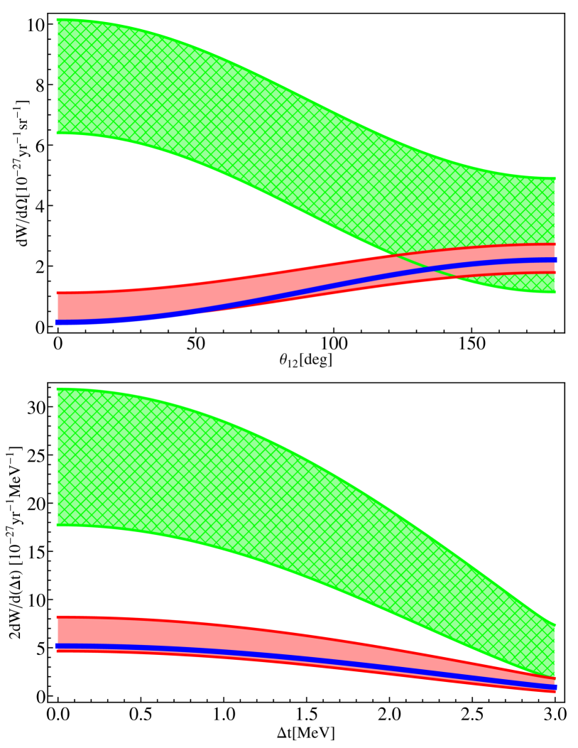
Figure 1: Electrons angular distribution (upper panel) and energy distributions (lower panel) for the competition between $\nu$ and $\eta$ mechanisms, Case 1 (see Sec. IV for a full description of the bands).

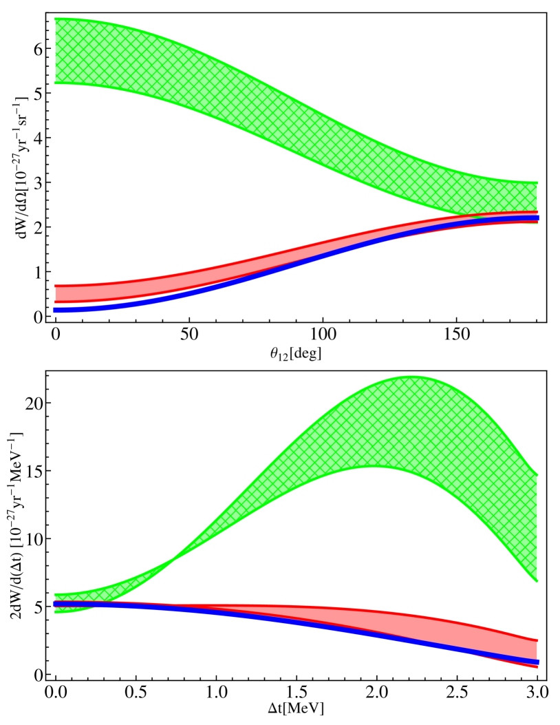
Figure 2: Same as Fig. 1 for the competition between $\nu$ and $\lambda$ mechanisms, Case 2.

IV Results

Here, we analyze in detail the two-electron angular and energy distributions for ⁸²Se, which was chosen as a baseline isotope by the SuperNEMO experiment Arnold and et al (2010); Bongrand (2015). We calculate the ⁸²Se NME of Eq. (25) using a shell model approach with the JUN45 Honma et al. (2009) effective Hamiltonian in the $jj44$ model space Sen’kov et al. (2014); Sen’kov and Horoi (2014). The nuclear structure effects are taken into account by the inclusion of short-range correlations with CD-Bonn parametrization, finite nucleon size effects, and higher order corrections of the nucleon current Horoi and Stoica (2010). We point out that some of the neutrino potentials in Eq. (26) are divergent Doi et al. (1985), such that the approximations $\chi_{GT\omega}=2-\chi_{GTq}$ and $\chi_{F\omega}=2\chi_{F}-\chi_{Fq}$ Tomoda (1991) are not accurate. This simplification was widely used because of the high complexity and difficulty of the previous shell model calculations with large model spaces Retamosa et al. (1995); Caurier et al. (1996) when most of $0\nu\beta\beta$ decaying isotopes were considered. A solution to this problem is to first perform the radial integral over the coordinate space and only after the second integral over the momentum space in Eq. (27). For $g_{A}$ we use the older value of 1.254 for an easier comparison to other NME and PSF results in the literature. It was shown in Ref. Sen’kov et al. (2014) that changing to the newer value of 1.27 Olive et al. (2014) changes the result by only 0.5%. Most of uncertainties in the shell model calculations come from different parametrization of the short range correlations, but they are less than 20% for most of the NME. It is also worth noting that the shell model NME are in general smaller by a factor of 2 than the QRPA NME, but recent work on restoring the broken symmetries in QRPA shows a tendency of reducing the QRPA values towards the shell model ones (see, e.g., Sec. IV.c of Ref. Horoi and Neacsu (2016a)).

The NME calculated in this work are presented on the first line of Table 1. The second line displays the normalized values $\chi_{\alpha}$ ($\alpha=F,GT\omega,F\omega,GTq,Fq,T,R,P$).

Table 1: The ⁸²Se NME corresponding to Eq. (24).

$M_{GT}$	$M_{F}$	$M_{GT\omega}$	$M_{F\omega}$	$M_{GTq}$	$M_{Fq}$	$M_{T}$	$M_{R}$	$M_{P}$
$2.993$	$-0.633$	$2.835$	$-0.618$	$3.004$	$-0.487$	$0.012$	$3.252$	$-1.286$
	$\chi_{F}$	$\chi_{GT\omega}$	$\chi_{F\omega}$	$\chi_{GTq}$	$\chi_{Fq}$	$\chi_{T}$	$\chi_{R}$	$\chi_{P}$
	$-0.134$	$0.947$	$-0.131$	$1.003$	$-0.103$	$0.004$	$1.086$	$0.430$

The values of the $\chi_{1\pm}$ and $\chi_{2\pm}$ factors of Eq. (23) are
$\chi_{1+}=0.717$, $\chi_{1-}=1.338$, $\chi_{2+}=0.736$, $\chi_{2-}=0.930$.

The PSF that enter in the components of Eq. (4) are calculated in this work using Eq. (33). These can be also calculated by a simple manipulation of Eq. (9), involving $\tilde{A}_{\pm k}$ defined in Appendix B. Using a new effective method to calculate PSF Horoi and Neacsu (2016b) in agreement with other recent results, we choose a value of 92 for the effective “screening factor” ($S_{f}$) that changes the charge of the daugther nucleus, $Z_{s}=\frac{S_{f}}{100}Z$. Reference Horoi and Neacsu (2016b) provides a detailed study of the $2\nu\beta\beta$ and $0\nu\beta\beta$ PSF using this method for 11 nuclei. In the case of $G_{1}$, we obtain results which are in good agreement with those of Ref. Stefanik et al. (2015), having a difference of about 8%. The results of Ref. Stefanik et al. (2015) have been obtained more rigorously by solving numerically the Dirac equation and by including the effects of the finite nuclear size and electron screening using a Coulomb potential derived from a realistic proton density distribution in the daughter nucleus. The largest difference is 15.5% in the case of $G_{8}$. The original formalism of Ref. Doi et al. (1985) provides significantly larger differences, of up to more than 64% for $G_{8}$ of ⁸²Se, and would result in differences in half-lives of over 30% for Case 4, where all the nine PSF contribute. However, given the larger uncertainty in the NME Brown et al. (2015), our approximation is satisfactory and we use it in calculations of the half-lives and of the two-electron angular and energy distributions.

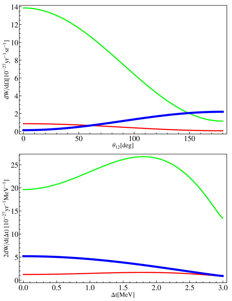
Figure 3: Same as Fig. 1 for the competition between $\lambda$ and $\eta$ mechanisms, Case 3.

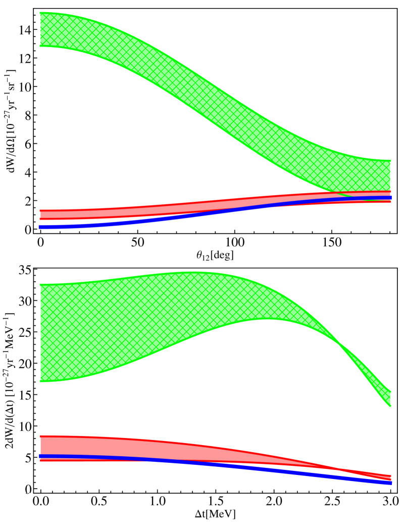
Figure 4: Same as Fig. 1 for the competition between $\nu$, $\lambda$ and $\eta$ mechanisms, Case 4.

Table 2: The ⁸²Se PSF corresponding to Eq. (33) expressed in $\left[\textmd{yr}^{-1}\right]$

$G_{1}\times 10^{14}$	$G_{2}\times 10^{14}$	$G_{3}\times 10^{14}$	$G_{4}\times 10^{15}$	$G_{5}\times 10^{13}$
$2.31$	$7.93$	$1.61$	$4.75$	$5.33$
	$G_{6}\times 10^{12}$	$G_{7}\times 10^{10}$	$G_{8}\times 10^{11}$	$G_{9}\times 10^{9}$
	$4.09$	$2.97$	$2.02$	$1.09$

In our analysis of the angular and energy distributions we consider five scenarios: a reference case named “Case 0”, commonly referred to in the literature as the “mass mechanism”(displayed with a thick blue line in all the figures); a case when only the mass mechanism and the $\eta$ mechanism contribute, presented as “Case 1”; the scenario when only the mass mechanism and the $\lambda$ mechanism contribute, “Case 2“; the case when the mass mechanism does not contribute and we have competition and interference between the $\lambda$ and the $\eta$ mechanisms denoted as ”Case 3“; and the most complex scenario, ”Case 4“, when there is competition and interference between all the mechanisms.

Table 3: The neutrino parameter values chosen for the five cases described in the text.

	$\left<\nu\right>$	$\left<\lambda\right>$	$\left<\eta\right>$
Case 0 Blue	$2\times 10^{-7}$	$0$	$0$
Case 1 Red	$2\times 10^{-7}$	$0$	$0.5\times 10^{-9}$
Case 1 Green	$2\times 10^{-7}$	$0$	$2\times 10^{-9}$
Case 2 Red	$2\times 10^{-7}$	$0.5\times 10^{-7}$	$0$
Case 2 Green	$2\times 10^{-7}$	$2\times 10^{-7}$	$0$
Case 3 Red	$0$	$0.5\times 10^{-7}$	$0.5\times 10^{-9}$
Case 3 Green	$0$	$2\times 10^{-7}$	$2\times 10^{-9}$
Case 4 Red	$2\times 10^{-7}$	$0.5\times 10^{-7}$	$0.5\times 10^{-9}$
Case 4 Green	$2\times 10^{-7}$	$2\times 10^{-7}$	$2\times 10^{-9}$

The values of the effective parameters for these scenarios are chosen such that they highlight the competition or the dominance of these mechanisms, taking into account the current experimental limits Barry and Rodejohann (2013); Stefanik et al. (2015) for the ⁷⁶Ge $0\nu\beta\beta$ half-life (see also Appendix A). They are presented in Table LABEL:cases. In the figures, the red color indicates the lower values for $\lambda$ or $\eta$, while the green color is used for the higher values.

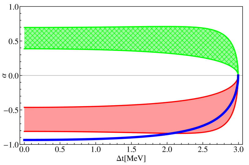
Figure 5: The angular correlation coefficient corresponding to Case 1. The meaning of the bands is the same as in Figs. $1-4$.

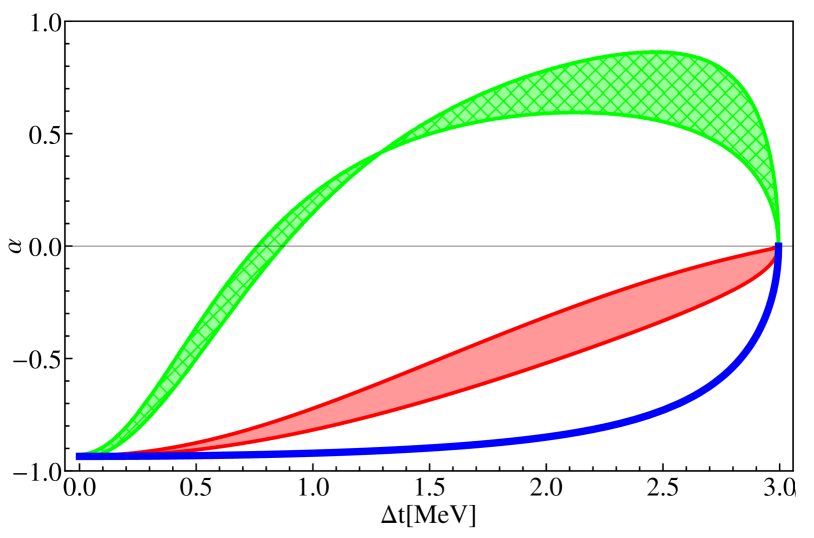
Figure 6: The angular correlation coefficient corresponding to Case 2. The meaning of the bands is the same as in Figs. 1-4.

For an easier evaluation of each contribution and the interference effects, we provide in Table LABEL:tab-ci the calculated $C_{i}$ factors ($i=1,\ldots,6$) of Eq. (22), together with their effective values from Eqs. (II), for each particular case. Due to the large $G_{7}$,$G_{8}$, and $G_{9}$ PSF, the contribution of $C_{5}$ has a significantly higher magnitude compared to the other factors, such that the calculations are very sensitive to the $\eta$ mechanism for the present limits of the neutrino physics parameters.

Table 4: The ⁸²Se $C_{i}$ factors ($i=1,\ldots,6$) corresponding to Eq. (4) expressed in $\left[yr^{-1}\right]$. We also present the effective values when these factors are multiplied with the neutrino parameters from the four cases discussed

	$C_{1}$	$C_{2}$	$C_{3}$	$C_{4}$	$C_{5}$	$C_{6}$
	$2.94\times 10^{-14}$	$-1.46\times 10^{-14}$	$4.75\times 10^{-12}$	$7.72\times 10^{-14}$	$1.15\times 10^{-9}$	$-1.01\times 10^{-13}$
	$C_{\nu^{2}}$	$C_{\nu\lambda}$	$C_{\nu\eta}$	$C_{\lambda^{2}}$	$C_{\eta^{2}}$	$C_{\lambda\eta}$
Case 0 Blue	$1.18\times 10^{-27}$	$0$	$0$	$0$	$0$	$0$
Case 1 Red	$1.18\times 10^{-27}$	$0$	$4.75\times 10^{-28}$	$0$	$2.86\times 10^{-28}$	$0$
Case 1 Green	$1.18\times 10^{-27}$	$0$	$1.90\times 10^{-27}$	$0$	$4.58\times 10^{-27}$	$0$
Case 2 Red	$1.18\times 10^{-27}$	$-1.46\times 10^{-28}$	$0$	$1.93\times 10^{-28}$	$0$	$0$
Case 2 Green	$1.18\times 10^{-27}$	$-5.83\times 10^{-28}$	$0$	$3.09\times 10^{-27}$	$0$	$0$
Case 3 Red	$0$	$0$	$0$	$1.93\times 10^{-28}$	$2.86\times 10^{-28}$	$-2.53\times 10^{-27}$
Case 3 Green	$0$	$0$	$0$	$3.09\times 10^{-27}$	$4.58\times 10^{-27}$	$-4.04\times 10^{-29}$
Case 4 Red	$1.18\times 10^{-27}$	$-1.46\times 10^{-28}$	$4.75\times 10^{-28}$	$1.93\times 10^{-28}$	$2.86\times 10^{-28}$	$-2.53\times 10^{-30}$
Case 4 Green	$1.18\times 10^{-27}$	$-5.83\times 10^{-28}$	$1.90\times 10^{-27}$	$3.09\times 10^{-27}$	$4.58\times 10^{-27}$	$-4.04\times 10^{-29}$

One may calculate the $0\nu\beta\beta$ half-life with either Eq. (4) using the nine PSF of Eq. (33) displayed in Table 2 or by integrating Eq. (7) over angles ($\theta_{12}$ from $0$ to $\pi$) and energy in Eq. (9) ($\Delta t$ goes from $0$ to $Q_{\beta\beta}$, which is $2.99$ MeV for ⁸²Se). The calculated half-lives for the cases of interest are presented in Table LABEL:half-lives. There are four combinations for the $CP$ phases $\phi_{1}$ and $\phi_{2}$, providing up to four values for the half-lives for each case. All half-lives in Table LABEL:half-lives, except Case 3 Red, are above the present experimental limits, but within the reach of the SuperNEMO experimental setup ($1.0\times 10^{26}$ years). One should also mention that the on-axis limits for the neutrino physics parameters $<\lambda>$ and $<\eta>$ corresponding to the same half-life, $9.41\times 10^{25}$ years, as the 100 meV mass mechanism are $1.2\times 10^{-7}$ and $1.0\times 10^{-9}$, respectively. The bands in the figures represent the interference effects of these phases, and their width is the maximum difference between them. In the case of the mass mechanism, there is no interference, such that Case 0 is represented by a single thick blue line. This line is present in all the figures to provide the reader with a reference scenario, which is the most studied in the literature. In the following, we discuss these cases.

Table 5: Calculated half-lives ($T_{1/2}$) for the four possible combinations of values for $\phi_{1}$ and $\phi_{2}$ in Eq. (4).

	$\phi_{1}=0,\phi_{2}=0$	$\phi_{1}=\pi,\phi_{2}=\pi$	$\phi_{1}=0,\phi_{2}=\pi$	$\phi_{1}=\pi,\phi_{2}=0$
Case 0 Blue	$9.41\times 10^{25}$	$9.41\times 10^{25}$	$9.41\times 10^{25}$	$9.41\times 10^{25}$
Case 1 Red	$5.72\times 10^{25}$	$1.12\times 10^{26}$	$1.12\times 10^{26}$	$5.72\times 10^{25}$
Case 1 Green	$1.45\times 10^{25}$	$2.87\times 10^{25}$	$2.87\times 10^{25}$	$1.45\times 10^{25}$
Case 2 Red	$9.05\times 10^{25}$	$7.31\times 10^{25}$	$9.05\times 10^{25}$	$7.31\times 10^{25}$
Case 2 Green	$3.01\times 10^{25}$	$2.29\times 10^{25}$	$3.01\times 10^{25}$	$2.29\times 10^{25}$
Case 3 Red	$2.32\times 10^{26}$	$2.32\times 10^{26}$	$2.30\times 10^{26}$	$2.30\times 10^{26}$
Case 3 Green	$1.45\times 10^{25}$	$1.45\times 10^{25}$	$1.44\times 10^{25}$	$1.44\times 10^{25}$
Case 4 Red	$5.59\times 10^{25}$	$8.36\times 10^{25}$	$1.07\times 10^{26}$	$4.86\times 10^{25}$
Case 4 Green	$1.09\times 10^{25}$	$1.48\times 10^{25}$	$1.73\times 10^{25}$	$9.75\times 10^{24}$

Case 0, representing the mass mechanism and displayed in the Figs. $1-4$ with a blue line, is the most studied mechanism in the literature. The value of the effective neutrino mass parameter $\left<\nu\right>=\left|\eta_{\nu}\right|$ is chosen to correspond to a neutrino mass limit of about 0.1 eV, which results in a calculated half-life of $9.4\times 10^{25}$, just beyond the current experimental limits but within the SuperNEMO reach Bongrand (2015). From Figs. $1-2$, one can see that this mode dominates the other contributions as long as $\left<\nu\right>\geq 4\times\left<\lambda\right>$ and $\left<\nu\right>\geq 400\times\left<\eta\right>$ (the red bands). Should any of the $\left<\lambda\right>$ or $\left<\eta\right>$ parameters increase four times (hatched green bands), the distributions change and one could identify the domination of another mechanism.

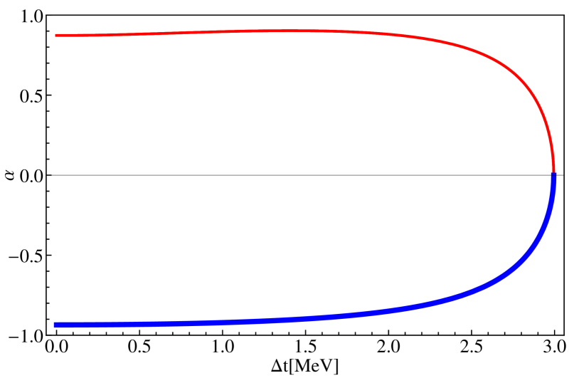
Figure 7: The angular correlation coefficient corresponding to Case 3. The meaning of the bands is the same as in Figs. $1-4$. The red and green (narrow) bands are overlapping.

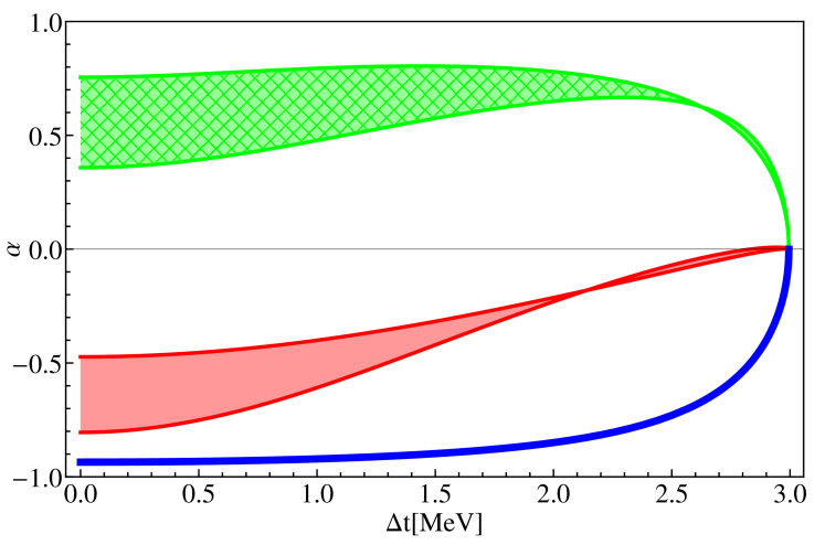
Figure 8: The angular correlation coefficient corresponding to Case 4. The meaning of the bands is the same as in Figs. $1-4$.

Case 1 presented in Fig. 1 describes the $\eta$ mechanism dominance (hatched green bands) showing a significant change in the shape of the angular distribution (Fig. 1, upper panel), while the energy distribution retains the shape of Case 0, only increasing in amplitude. In the scenario of Case 2 presented in Fig. 2, one can see the dominance of the $\lambda$ mechanism (hatched green bands) in both distributions as changes in the shape and amplitude. One can conclude that one can use these different shape changes to distinguish between $\left<\nu\right>$, $\left<\lambda\right>$, and $\left<\eta\right>$ mechanism dominance, assuming that only two of them can compete.

However, one needs to consider the case when the $|m_{ee}|=m_{e}\left<\nu\right>$ is very small or zero, while the $\lambda$ and $\eta$ mechanisms are competing. This scenario is covered by Case 3 presented in Fig. 3. The interference term $C_{\lambda\eta}$ is very small leading to very narrow interference bands. Dominance of any of the two mechanisms would show little difference from the similar behavior shown in Figs. 1 and 2 (the shape is fixed by the small interference term, while in Case 1 and 2 the dependence on the interference phases could distort the shapes). The green lines in Case 3 are just rescaling of the red to emphasize the effect of rescaling relative to the standard mass mechanism (blue line). The shapes of the distributions and their changes seem to be similar to some of those in Fig. 2. However, the ratio max/min in the angular distribution (15/1 for Case 3 vs 2/1 for Case 2) could be used to distinguish between these two cases.

Case 4 allows competition between all three contributions (Fig. 4). Obviously, the qualitative behavior of these distributions cannot be easily disentangled from those of Cases $1-3$ discussed above. That would require a numerical simulation that includes interference effects to rule in or out some of these scenarios.

One should also mention that the energy distribution of the angular correlation coefficient, $\alpha=B(\epsilon)/A(\epsilon)$ in our Eq. (7), could provide additional information (see, e.g., Figs. $6.5-6.9$ of Doi et al. (1985) and Fig. 7 of Stefanik et al. (2015)). Figures $5-8$ show the angular correlation coefficient $\alpha(\Delta t)$ of all four cases analyzed in Figs. $1-4$. One can clearly see that Cases 2 and 3 can also be identified by the value of $\alpha$ when the energies of the two emitted electrons are very close ($\Delta t\approx 0$). Cases 3 and 1 can be separated by the shape of their energy distributions. Figures $5-8$ show that the angular correlation coefficient could be also used to better identify the other cases analyzed in Figs. $1-4$.

Given the complexity of our analysis, and considering the potential usefulness for future analyses, we provide a link to a Mathematica file that can be used to perform these calculations and produce the plots included in this paper edi .

Table 6: Calculated limits of half-lives ratios, Eq. (14), for different combinations of isotopes (see text for details). For example, in the combination Ge/Se (1) corresponds to Ge and (2) to Se.

	Ge/Se		Ge/Te		Ge/Xe		Se/Te		Se/Xe		Te/Xe
	Ge	Se	Ge	Te	Ge	Xe	Se	Te	Se	Xe	Te	Xe
$G^{0\nu}_{01}\times 10^{14}$	0.237	1.018	0.237	1.425	0.237	1.462	1.018	1.425	1.018	1.462	1.425	1.462
$M^{0\nu}(1/2)$	3.57	3.39	3.57	1.93	3.57	1.76	3.39	1.93	3.39	1.76	1.93	1.76
$M^{0N}(1/2)$	202	187	202	136	202	143	187	136	187	143	136	143
$T_{1/2}^{\nu}(1)/T_{1/2}^{\nu}(2)$	3.87		1.76		1.50		0.45		0.39		0.85
$T_{1/2}^{N}(1)/T_{1/2}^{N}(2)$	3.68		2.73		3.09		0.74		0.84		1.13
$R(N/\nu)$ present	0.95		1.55		2.06		1.63		2.17		1.33
$R(N/\nu)$ Faessler et al. (2014)	1.02		1.39		1.42		1.36		1.39		1.03

V Disentangling the heavy neutrino contribution

As mentioned in Sec. II, if the $\eta_{\lambda}$ and $\eta_{\eta}$ contributions could be ruled out by the two-electron energy and angular distributions analyzed in the previous section, and in that case assuming a seesaw type I dominance Bhupal Dev et al. (2015) the half-life is given by Eq. (3). Then, the relative contribution of the $\eta_{\nu}$ and $\eta^{R}_{N_{R}}$ terms can be identified if one measures the half-life of at least two isotopes Faessler et al. (2011); Vergados et al. (2012), provided that the corresponding matrix elements $M^{0\nu}$ and $M^{0N}$ are known with good precision. References Faessler et al. (2011); Vergados et al. (2012) already provided some limits of the ratios of the half-lives of different isotopes based on older QRPA calculations. However, based on those calculations, the two limits for $r(\nu/N)\equiv T_{1/2}^{\nu/N}(1)/T_{1/2}^{\nu/N}(2)$

$$r(\nu/N)=\frac{G^{0\nu}_{01}(2)\left|M^{0\nu/N}(2)\right|^{2}}{G^{0\nu}_{01}(1)\left|M^{0\nu/N}(1)\right|^{2}},$$ (14)

were too close to allow for a good separation of the contribution of these two mechanisms. In Eq. (14), terms $(1)$ and $(2)$ designate members of a pair of isotopes. Below, we present the results based on our shell model calculations given in Tables III and IV of Ref. Neacsu and Horoi (2015). In Table LABEL:hlrtable, Ge, Se, Te, and Xe are short-hand notions for ⁷⁶Ge, ⁸²Se, ¹³⁰Te, and ¹³⁶Xe, respectively. In the table, we only use the NME calculated with CD-Bonn short-range correlations. The $G^{0\nu}_{01}$ factors from Table III of Ref. Stefanik et al. (2015) were used (they are very close to those of Ref. Mirea et al. (2014)).

The pre-last line in Table LABEL:hlrtable presents the ratio of the ratios of half-lives, $R(N/\nu)=r(N)/r(\nu)$, calculated with our NME. One can see that the largest ratio is obtained for the combination ⁸²Se/¹³⁶Xe. Its magnitude larger than 2 indicates that one can differentiate between these two limits if the half-lives are known with reasonable uncertainties and provided that the NME can be calculated with sufficient precision. The last line in Table LABEL:hlrtable shows the same quantity calculated with the recent QRPA NME taken from Table I (columns d) of Ref. Faessler et al. (2014). On can see that these ratios are not as favorable in identifying the two limits. This analysis emphasizes again the need of having reliable NME for all mechanisms.

VI Conclusions

In this paper, we calculate nuclear matrix elements, phase-space factors, and half-lives for the $\ 0\nu\beta\beta\left(0^{+}\rightarrow 0^{+}\right)$ decay of ⁸²Se under different scenarios that include, besides the mass mechanism, the mixed right-handed/left-handed currents contributions known as $\eta$ and $\lambda$ mechanisms. For the mass mechanism dominance scenario, the results are consistent with previous calculations Sen’kov et al. (2014) using the same Hamiltonian. Inclusion of contributions from $\eta$ and $\lambda$ mechanisms have the tendency to decrease the half-lives.

We present the two-electrons angular and energy distributions for five theoretical scenarios of mixing between mass mechanisms contributions and $\eta$ and $\lambda$ mechanism contributions. From the figures presented in the paper, one can recover the general conclusion Doi et al. (1985) that the energy distribution can be used to distinguish between the mass mechanism and the $\lambda$ mechanism, while the angular distribution can be used in addition to the energy distribution to distinguish between the mass mechanism and the $\eta$ mechanism, but the identification could be more nuanced due to the lack of knowledge of the interference phases. In the case of the energy distributions for the mass mechanism dominance (blue line) and the $\lambda$ mechanism dominance (green band in Figure 2, lower panel), we find similar results to those of Fig. 2 in Ref. Arnold and et al (2010). However, our results emphasize the significant role of the interference phases $\phi_{1}$ and $\phi_{2}$ in identifying the effect.

We also find out from the analysis of Case 3 that if the effective neutrino mass is very small, close to zero, and the $\eta$ and $\lambda$ mechanisms are competing, then one can potentially identify this scenario from the $\lambda$ dominance, Case 2, by comparing the ratio min-to-max in the angular distributions and/or by the behavior of the angular correlation coefficient for almost equal electron energies. The small interference effects in Case 3 could be also used as an additional identification tool. These conclusions seem to be stable even if one considers small NME changes, such as those due to different short-range correlations models.

We conclude that the $\eta$ mechanism, if it exists, may be favored to compete with the mass mechanisms due to the larger contribution from the phase-space factors. Reference Barry and Rodejohann (2013) shows however that it is possible to obtain a $\lambda$ mechanism dominance in some cases.

Finally we show that if the $\eta_{\lambda}$ and $\eta_{\eta}$ contributions could be ruled out by the two-electron energy and angular distributions, the mass mechanisms can be disentangled from the heavy right-handed neutrino-exchange mechanism using ratios of half-lives of few isotopes. The analysis based on our shell model NME indicates that the most favorable combinations of isotopes would be ⁸²Se/¹³⁶Xe and ⁷⁶Ge/¹³⁶Xe.

Certainly, the analysis presented in this paper is based on the positive detection of the neutrinoless double-beta decay, followed by the collection of enough events that one can use to make assessments on the angular and energy distributions. Similar distributions were obtained with high precision by NEMO-3 for the $2\nu\beta\beta$ of ¹⁰⁰Mo, but a very large number, about 1 million, of events were collected Bongrand (2015). Clearly, this large number of events will not be available for any $0\nu\beta\beta$ experiment, but we believe that the tools provided by our analysis could help to assess probabilities for these mechanisms even if only tens of events are collected.

Appendix A Left-right symmetric model

Left-right symmetric models Pati and Salam (1974); Mohapatra and Pati (1975); Senjanovic and Mohapatra (1975); Keung and Senjanovic (1983) could explain the physics of the right-handed currents, which may contribute to the neutrinoless double-beta decay process, and are also under current investigation at LHC Khachatryan et al. (2014). Specific details for double-beta decay can be found in Ref. Barry and Rodejohann (2013).

The neutrino mixing matrices are defined by

$$n^{\prime}_{L}=\binom{\nu^{\prime}_{L}}{{\nu^{\prime}_{R}}^{c}}=\binom{U\ S}{T\ V}\binom{\nu_{L}}{N_{R}^{c}},$$ (15)

where $\nu^{\prime}_{L}$, ${\nu^{\prime}_{R}}^{c}$ are flavor eigenstates, and $\nu_{L}$, $N_{R}^{c}$ are mass eigenstates. Here, the $U$ and $V$ matrices are almost unitary, while the $S$ and $T$ matrices are very small. The sterile neutrinos $\nu^{\prime}_{R}$ and the mass eigenstates $N_{R}$ are presumed to be very heavy, but at least the lightest ones are at the TeV scale. Light (1 eV) sterile neutrinos could exist, and they could influence the effective neutrino mass and the outcome of $0\nu\beta\beta$ decay Vergados et al. (2012), but they may be detected in neutrino oscillations experiments. The neutrino physics parameter $\left|\left<m_{ee}\right>\right|\equiv\left|\sum U_{ek}^{2}m_{k}\right|$ is the effective electron neutrino mass, and the suitably normalized dimensionless parameter that describes lepton number violation is (the upper limits for the neutrino physics parameters below were taken from Refs. Stefanik et al. (2015); Barry and Rodejohann (2013))

$$\left|\eta_{\nu}\right|=\frac{\left|\left<m_{ee}\right>\right|}{m_{e}}=\frac{\left|\sum_{k}^{light}U_{ek}^{2}m_{k}\right|}{m_{e}}\lesssim 7\times 10^{-7},$$ (16)

with $U_{ei}$ the (PMNS) mixing matrix of light neutrinos, $m_{i}$ the light neutrino masses, and $m_{e}$ the electron mass. For the mixing of the left- and right-handed currents with the heavy neutrino the neutrino physics parameters in the left-right symmetric model are given by

$$\left|\eta^{L}_{N_{R}}\right|=m_{p}\left|\sum_{k}^{heavy}\frac{{S_{ek}}^{2}}{M_{k}}\right|\lesssim 7\times 10^{-9},$$ (17)

$$\left|\eta^{R}_{N_{R}}\right|=m_{p}\left(\frac{m_{W_{L}}}{m_{W_{R}}}\right)^{4}\left|\sum_{k}^{heavy}\frac{{V^{\star}_{ek}}^{2}}{M_{k}}\right|\lesssim 7\times 10^{-9},$$ (18)

where $m_{W_{R}}\ (m_{W_{L}})$ is the mass of the right-handed $W_{R}\ (\textmd{left-handed}\ W_{L})$, $M_{i}$ are the masses of the heavy neutrinos, and $V$ is the right-handed analogue of the PMNS matrix U. To satisfy the present limit of $\left|\eta^{R}_{N_{R}}\right|$, one needs $m_{W_{R}}$ and some of the $M_{k}$ masses at TeV scale. For the terms that could contribute to the neutrinoless double-beta decay that involve a mixture of left-handed and right-handed currents, the $\eta_{\lambda}$ and $\eta_{\eta}$ neutrino physics parameters are

$$\left|\eta_{\lambda}\right|=\left(\frac{m_{W_{L}}}{m_{W_{R}}}\right)^{2}\left|\sum_{k}^{light}U_{ek}T^{\star}_{ek}\right|\lesssim 4\times 10^{-7}\ ,$$ (19)

$$\left|\eta_{\eta}\right|=\textmd{tan}\xi\left|\sum_{k}^{light}U_{ei}T^{\star}_{ek}\right|\lesssim 3\times 10^{-9}\ .$$ (20)

The heavy neutrino contributions to both $\lambda$ and $\eta$ mechanisms are suppressed, being proportional to $\sum_{k}^{heavy}S_{ek}V^{\star}_{ek}q/M^{2}_{k}$.

The $CP$ phases used in Eq. (4) are

$$\phi_{1} = \text{arg}\left[\left(\sum_{k}^{light}U_{ek}^{2}m_{k}\right)\left(\left(\frac{M_{W_{L}}}{M_{W_{R}}}\right)^{2}\sum_{k}^{light}U_{ek}V_{ek}\right)^{\star}\right],$$

$$\phi_{2} = \text{arg}\left[\left(\sum_{k}^{light}U_{ek}^{2}m_{k}\right)\left(\xi\sum_{k}^{light}U_{ek}V_{ek}\right)^{\star}\right].$$ (21)

Appendix B $0\nu\beta\beta$ NME

Most of the theoretical formalism used in this work is adopted from Refs. Doi et al. (1985) and Suhonen and Civitarese (1998), with little change of notation for simplicity and consistency wherever need.

The $C_{1-6}$ factors composed from PSF and NME Doi et al. (1985) are

$$C_{1} =\left(1-\chi_{F}\right)^{2}G_{1},$$ (22a)

$$C_{2} =-\left(1-\chi_{F}\right)\left[\chi_{2-}G_{3}-\chi_{1+}G_{4}\right],$$ (22b)

$$C_{3} =\left(1-\chi_{F}\right)$$

$$\times\left[\chi_{2+}G_{3}-\chi_{1-}G_{4}-\chi_{P}G_{5}+\chi_{R}G_{6}\right],$$ (22c)

$$C_{4} =\left[\chi_{2-}^{2}G_{2}+\frac{1}{9}\chi_{1+}^{2}G_{4}-\frac{2}{9}\chi_{1+}\chi_{2-}G_{3}\right],$$ (22d)

$$C_{5} =\chi_{2+}^{2}G_{2}+\frac{1}{9}\chi_{1-}^{2}G_{4}-\frac{2}{9}\chi_{1-}\chi_{2+}G_{3}+\chi_{P}^{2}G_{8}$$

$$-\chi_{P}\chi_{R}G_{7}+\chi_{R}^{2}G_{9},$$ (22e)

$$C_{6} =-2\left[\chi_{2-}\chi_{2+}G_{2}-\frac{1}{9}(\chi_{1+}\chi_{2+}+\chi_{2-}\chi_{1-})G_{3}\right.$$

$$+\left.\frac{1}{9}\chi_{1+}\chi_{1-}G_{4}\right],$$ (22f)

$$\chi_{1\pm} =\chi_{GTq}\pm 3\chi_{Fq}-6\chi_{T},$$ (23a)

$$\chi_{2\pm} =\chi_{GT\omega}\pm\chi_{F\omega}-\frac{1}{9}\chi_{1\pm}.$$ (23b)

The normalized NME

$$\chi_{\alpha}=M_{\alpha}/M_{GT}^{0\nu},$$ (24)

where $\alpha=F,T,GT\omega,F\omega,GTq,Fq,R$, and $P$. All Fermi-type matrix elements $M_{F(\omega q)}$ are multiplied by $g_{V}/g_{A}$.

Due to the two-body nature of the transition operator, the matrix elements are reduced to sums of products of two-body transition densities (TBTD) and matrix elements for two-particle states Horoi and Stoica (2010):

$$M_{\alpha}^{0\nu} = \sum_{j_{p}j_{p^{\prime}}j_{n}j_{n^{\prime}}J_{\pi}}TBTD\left(j_{p}j_{p^{\prime}},j_{n}j_{n^{\prime}};J^{\pi}\right)$$ (25)

$$\times \left<j_{p}j_{p^{\prime}};J^{\pi}\|\tau_{-1}\tau_{-2}O^{\alpha}_{12}\|j_{n}j_{n^{\prime}};J^{\pi}\right>.$$

The detailed expressions for the two-body transition operators $(O^{\alpha}_{12})$ can be found in Ref. Muto et al. (1989). They can be factorized into products of coupling constants and operators which act on the intrinsic spin, relative and center-of-mass wave functions of two-particle states Horoi and Stoica (2010).

The NME depend on four dimensionless neutrino potentials defined by the integral over the momentum of the virtual neutrino. Expressions for the Gamow-Teller (GT), the Fermi (F), and the tensor (T) cases are described in detail in Refs. Horoi and Stoica (2010); Sen’kov and Horoi (2013). The other three potentials are presented here in a form similar to Eq. (12) of Ref. Muto et al. (1989),

$$H_{\omega}^{0\nu}(r)=\frac{2R}{\pi}\int_{0}^{\infty}\frac{q^{2}j_{0}(qr)\textmd{d}q}{\left(q+\left<E\right>\right)^{2}}\equiv\int_{0}^{\infty}q^{2}j_{0}(qr)V_{\omega}(q)\textmd{d}q,$$ (26a)

$$\textmd{for the }M^{0\nu}_{GTw}\textmd{ and }M^{0\nu}_{Fw}\textmd{ NME,}$$

$$H_{q}^{0\nu}(r)=\frac{2R}{\pi}\int_{0}^{\infty}\frac{q^{2}j_{1}(qr)\textmd{d}q}{q+\left<E\right>}\equiv\int_{0}^{\infty}q^{2}j_{1}(qr)V_{q}(q)\textmd{d}q,$$ (26b)

$$\textmd{for the }M^{0\nu}_{GTq},M^{0\nu}_{Fq},M^{0\nu}_{T},\textmd{ and }M^{0\nu}_{P}\textmd{ NME}.$$

$$\textmd{In the case of }M^{0\nu}_{R},\textmd{ the potential is written as:}$$

$$H_{R}^{0\nu}(r)=\frac{2R^{2}}{\pi M}\int_{0}^{\infty}\frac{q^{3}j_{0}(qr)\textmd{d}q}{q+\left<E\right>}\equiv\int_{0}^{\infty}q^{2}j_{0}(qr)V_{\omega}(q)\textmd{d}q,$$ (26c)

where $M$ is the nucleon mass, $R$ the nuclear radius ($R=1.2A^{1/3}fm$), $\left<E\right>$ represents the closure energy, $V_{\omega,q,R}$ are the Fourier transforms of the potentials, and $j_{\kappa}(qr)$ are spherical Bessel functions of rank $\kappa$. Due to the small contribution of the $\chi_{P}$ term, we take a typical value of 0.5 for the associated normalized NME.

The computation of the matrix element requires solving a double integral over the coordinate space and over the momentum [from Eq. (26)] of the form Neacsu et al. (2012)

$$\mathcal{I}_{\alpha}(\mu;m)=\int_{0}^{\infty}q^{2}dq\ V_{\alpha}(q)$$ (27)

$$\times\left(\frac{2}{\pi}\right)^{\frac{1}{2}}\left(2\nu\right)^{\frac{m+1}{2}}\int_{0}^{\infty}dr\ e^{-\mu r^{2}}r^{m}j_{\kappa}(qr)$$

where $\mu$ = $\nu$, $\nu+a$, $\nu+2a$, with $\nu$ the oscillator constant and $m$ is an integer.

It was previously observed in Ref. Doi et al. (1985) that the three potentials in Eq. (26) are formally divergent but the associated radial matrix elements are not, if certain precautions are taken, such as first performing the radial integrals and then the integrals of the momentum in Eq. (27), as was done in Ref. Horoi and Stoica (2010).

In Ref. Sen’kov et al. (2014), a method was proposed for obtaining an optimal closure energy, which yields similar results as when preforming calculations beyond the closure approximation. Here, we use an optimal average closure energy $\left<E\right>$ of $3.4$ MeV, which has been shown to produce accurate results in the case of $M_{GT}$ and $M_{F}$ (see Fig. 5 of Ref. Sen’kov et al. (2014)). Therefore, our NME do not have any significant uncertainties related to choice of the closure energy. Higher order corrections of the nuclear current for the Gamow Teller nuclear matrix element and CD-Bonn parametrization short-range correlations are taken into account as described in Ref. Horoi and Stoica (2010).

To calculate the two-electron angular and relative energy distributions, we take into account the decay rate as described by Eq. (C$\cdot$3$\cdot$1) of Ref. Doi et al. (1985). This leads to the expressions of Eqs. (7) and (8). The factors $N_{1-4}(\epsilon_{1})$ represent mixtures of NME and PSF, expressed as

$$N_{1}(\epsilon_{1}) =a_{\textmd{-}1\textmd{-}1}^{*}\left[\left(Z_{1}-\frac{4Z_{6}}{3}\right)-\left(\frac{4}{m_{e}R}\right)\left(Z_{4}-\xi\frac{Z_{6}}{6}\right)\right],$$ (28a)

$$N_{2}(\epsilon_{1}) =a_{11}^{*}\left[\left(Z_{1}-\frac{4Z_{6}}{3}\right)+\left(\frac{4}{m_{e}R}\right)\left(Z_{4}-\xi\frac{Z_{6}}{6}\right)\right],$$ (28b)

$$N_{3}(\epsilon_{1}) =a_{1-1}^{*}\left[\left(Z_{1}-\frac{2Z_{5}}{3}\right)-\left(\frac{\epsilon_{12}}{m_{e}}\right)\left(Z_{3}+\frac{Z_{5}}{3}\right)\right],$$ (28c)

$$N_{4}(\epsilon_{1}) =a_{-11}^{*}\left[\left(Z_{1}-\frac{2Z_{5}}{3}\right)+\left(\frac{\epsilon_{12}}{m_{e}}\right)\left(Z_{3}+\frac{Z_{5}}{3}\right)\right],$$ (28d)

with $\xi=3\alpha Z_{s}+(T+2)m_{e}R$, $\epsilon_{12}=\epsilon_{1}-\epsilon_{2}$ and $a_{\kappa\lambda}=\tilde{A}_{\kappa}(\epsilon_{1})\tilde{A}_{\lambda}(\epsilon_{2})$, where $\epsilon_{2}=T+2-\epsilon_{1}.$

$$\tilde{A}_{\pm k}(\epsilon)\cong\sqrt{(\epsilon\mp m_{e})/2\epsilon}\sqrt{F_{k-1}(Z_{s},\epsilon)}.$$ (29)

$$F_{k-1}(Z_{s},\epsilon) = \left[\frac{\Gamma(2k+1)}{\Gamma(k)\Gamma(2\gamma_{k}+1)}\right]^{2}$$ (30)

$$\times (2pR)^{2(\gamma_{k}-k)}|\Gamma(\gamma_{k}+iy)|^{2}e^{\pi y}$$

$$\gamma_{k}=\sqrt{k^{2}-(\alpha Z)^{2}},\qquad y=\alpha Z_{s}\epsilon/p,$$ (31)

where $\alpha$ is the fine structure constant, $p_{i}=\sqrt{\epsilon_{i}^{2}-1}($with $i=1,2)$, and $Z_{s}=Z\cdot\frac{S_{f}}{100}$ the ”screened“ charge of the final nucleus, and $S_{f}=92$ is the effective ”screening“ factor from Table 4 of Ref. Horoi and Neacsu (2016b). Here, $Z_{1-6}$ are composed of the NME from Eq. (25), defined as follows:

$$Z_{1} =(\left<\nu\right>)(\chi_{F}-1)M_{GT}^{0\nu},$$ (32a)

$$Z_{3} =\left[-\left<\lambda\right>(\chi_{GT\omega}-\chi_{F\omega})e^{-i\phi_{1}}\right.$$ (32b)

$$+\left.\left<\eta\right>(\chi_{GT\omega}+\chi_{F\omega})e^{-i\phi_{2}}\right]M_{GT}^{0\nu},$$ (32c)

$$Z_{4} =\left<\eta\right>\chi_{R}e^{-i\phi_{2}}M_{GT}^{0\nu},$$ (32d)

$$Z_{5} =\frac{1}{3}\left[\left<\lambda\right>\chi_{1+}e^{-i\phi_{1}}-\left<\eta\right>\chi_{1-}e^{-i\phi_{2}}\right]M_{GT}^{0\nu},$$ (32e)

$$Z_{6} =\left<\eta\right>\chi_{P}e^{-i\phi_{2}}M_{GT}^{0\nu}.$$ (32f)

Appendix C $0\nu\beta\beta$ decay PSF expressions

The PSF are calculated using the following expression adopted from Eq. (A.27) of Ref. Suhonen and Civitarese (1998):

$$G_{k}=\frac{a_{0\nu}}{\textmd{ln}2(m_{e}R)^{2}}\int\limits_{1}^{T+1}b_{k}F_{0}(Z_{s},\epsilon_{1})F_{0}(Z_{s},\epsilon_{2})\omega_{0\nu}(\epsilon_{1})\text{d}\epsilon_{1},$$ (33)

where $R$ is the nuclear radius ($R=r_{0}A^{1/3}$, with $r_{0}=1.2$ fm) and $F_{0}$ is defined in Eq. (30) for $k=1$.

$$a_{0\nu}=\frac{g_{A}^{4}\left(G_{F}\textmd{cos}\theta_{c}\right)^{4}m_{e}^{9}}{32\pi^{5}},$$ (34)

with $G_{F}=1.1663787\times 10^{-5}\ GeV^{-2}$ the Fermi constant, and $\textmd{cos}\theta_{c}=0.9749$ the Cabbibo angle. In Ref. Suhonen and Civitarese (1998), the constant $g^{0\nu}=a_{0\nu}/\textmd{ln}2=2.8\times 10^{-22}g_{A}^{4}\ yr^{-1}$ was used. Taking into account the value $g_{A}=1.27$, instead of $g_{A}=1.254$, would change the results by $5\%$. One should mention that the $G^{0\nu}_{01}g^{4}_{A}$ product in Eq. 3 is equal to $G_{1}$. Also, in Eq. (C1)

$$\omega_{0\nu}(\epsilon_{1})=p_{1}p_{2}\epsilon_{1}\epsilon_{2},$$ (35)

with $\epsilon_{2}=T+2-\epsilon_{1}$, $p_{1,2}=\sqrt{\epsilon_{1,2}^{2}-1}$, and $T$ defined in Eq. (10).

The kinematical factors $b_{k}$ are defined as

$$\ \ \ \ b_{1} =1,$$ (36)

$$\ \ \ \ b_{2} =\frac{1}{2}\left(\frac{\epsilon_{1}\epsilon_{2}-1}{\epsilon_{1}\epsilon_{2}}\right)(\epsilon_{1}-\epsilon_{2})^{2},$$ (37)

$$\ \ \ \ b_{3} =(\epsilon_{1}-\epsilon_{2})^{2}/\epsilon_{1}\epsilon_{2},$$ (38)

$$\ \ \ \ b_{4} =\frac{2}{9}\left(\frac{\epsilon_{1}\epsilon_{2}-1}{\epsilon_{1}\epsilon_{2}}\right),$$ (39)

$$\ \ \ \ b_{5} =\frac{4}{3}\left(\frac{(T+2)\xi}{2r_{A}\epsilon_{1}\epsilon_{2}}-\frac{\epsilon_{1}\epsilon_{2}+1}{\epsilon_{1}\epsilon_{2}}\right),$$ (40)

$$\ \ \ \ b_{6} =\frac{4(T+2)}{r_{A}\epsilon_{1}\epsilon_{2}},$$ (41)

$$\ \ \ \ b_{7} =\frac{16}{3}\frac{1}{r_{A}\epsilon_{1}\epsilon_{2}}\left(\frac{\epsilon_{1}\epsilon_{2}+1}{2r_{A}}\xi-T-2\right),$$ (42)

$$\ \ \ \ b_{8} =\frac{2}{9}\frac{1}{(r_{A})^{2}\epsilon_{1}\epsilon_{2}}\left[(\epsilon_{1}\epsilon_{2}+1)(\xi^{2}+4(r_{A})^{2})\right.$$

$$\left.-4r_{A}\xi(T+2)\right],$$ (43)

$$\ \ \ \ b_{9} =\frac{8}{(r_{A})^{2}}\left(\frac{\epsilon_{1}\epsilon_{2}+1}{\epsilon_{1}\epsilon_{2}}\right),$$ (44)

with $\xi=3\alpha Z_{s}+r_{A}(T+2)$, where $\alpha$ represents the fine structure constant, $Z_{s}=Z\cdot\frac{S_{f}}{100}$ the ”screened” charge of the final nucleus, and $r_{A}=m_{e}R$.

In Eq. (2), Eq. (3), Eq. (14) and in Table LABEL:hlrtable we use the factor $G_{01}^{0\nu}=G_{1}/\left(g_{A}\right)^{4}$.

References

- Schechter and Valle (1982) J. Schechter and J. W. F. Valle, Phys. Rev. D 25, 2951 (1982).
- Nieves (1984) J. Nieves, Phys. Lett. B 147, 375 (1984).
- Takasugi (1984) E. Takasugi, Phys. Lett. B 149, 372 (1984).
- Hirsch et al. (2006) M. Hirsch, S. Kovalenko, and I. Schmidt, Phys. Lett. B 642, 106 (2006).
- Vergados et al. (2012) J. D. Vergados, H. Ejiri, and F. Simkovic, Rep. Prog. Phys. 75, 106301 (2012).
- Horoi (2013) M. Horoi, Phys. Rev. C 87, 014320 (2013).
- Keung and Senjanovic (1983) W.-Y. Keung and G. Senjanovic, Phys. Rev. Lett. 50, 1427 (1983).
- Barry and Rodejohann (2013) J. Barry and W. Rodejohann, J. High Energy Phys. p. 153 (2013).
- Deppisch et al. (2016) F. F. Deppisch, M. Hirsch, and H. Pas, Phys. Rev. D 93, 013011 (2016).
- Neacsu and Horoi (2015) A. Neacsu and M. Horoi, Phys. Rev. C 91, 024309 (2015).
- Brown et al. (2014) B. A. Brown, M. Horoi, and R. A. Sen’kov, Phys. Rev. Lett. 113, 262501 (2014).
- Sen’kov and Horoi (2014) R. A. Sen’kov and M. Horoi, Phys. Rev. C 90, 051301(R) (2014).
- Sen’kov et al. (2014) R. A. Sen’kov, M. Horoi, and B. A. Brown, Phys. Rev. C 89, 054304 (2014).
- Sen’kov and Horoi (2013) R. A. Sen’kov and M. Horoi, Phys. Rev. C 88, 064312 (2013).
- Horoi and Brown (2013) M. Horoi and B. A. Brown, Phys. Rev. Lett. 110, 222502 (2013).
- Neacsu et al. (2012) A. Neacsu, S. Stoica, and M. Horoi, Phys. Rev. C 86, 067304 (2012).
- Horoi and Stoica (2010) M. Horoi and S. Stoica, Phys. Rev. C 81, 024321 (2010).
- Horoi et al. (2007) M. Horoi, S. Stoica, and B. A. Brown, Phys. Rev. C 75, 034303 (2007).
- Mitra et al. (2012) M. Mitra, G. Senjanovic, and F. Vissani, Nucl. Phys. B 856, 26 (2012).
- Blennow et al. (2010) M. Blennow, E. Fernandez-Martinez, J. Lopez-Pavon, and J. Menendez, JHEP 07, 096 (2010).
- Pati and Salam (1974) J. Pati and A. Salam, Phys. Rev. D 10, 275 (1974).
- Mohapatra and Pati (1975) R. Mohapatra and J. Pati, Phys. Rev. D 11, 2558 (1975).
- Senjanovic and Mohapatra (1975) G. Senjanovic and R. N. Mohapatra, Phys. Rev. D 12, 1502 (1975).
- Khachatryan et al. (2014) V. Khachatryan, A. M. Sirunyan, A. Tumasyan, W. Adam, T. Bergauer, M. Dragicevic, J. Erö, C. Fabjan, M. Friedl, R. Fruhwirth, et al. (CMS-Collaboration), Eur. Phys. J. C 74, 3149 (2014).
- Faessler et al. (2011) A. Faessler, A. Meroni, S. T. Petcov, F. Simkovic, and J. Vergados, Phys. Rev. D 83, 113003 (2011).
- Holt and Engel (2013) J. D. Holt and J. Engel, Phys. Rev. C 87, 064315 (2013).
- Doi et al. (1985) M. Doi, T. Kotani, and E. Takasugi, Prog. Theor. Phys. Suppl. 83, 1 (1985).
- Arnold and et al (2010) R. Arnold and et al, Eur. Phys. J. C 70, 927 (2010).
- Prezeau et al. (2003) G. Prezeau, M. Ramsey-Musolf, and P. Vogel, Phys.Rev. D 68, 034016 (2003).
- Gehman and Elliott (2007) M. Gehman, V and R. Elliott, S, J. Phys. G 34, 667 (2007).
- Bhattacharyya et al. (2003) G. Bhattacharyya, H. V. Klapdor-Kleingrothaus, H. Pas, and A. Pilaftsis, Phys. Rev. D 67, 113001 (2003).
- Deppisch and Päs (2007) F. Deppisch and H. Päs, Phys. Rev. Lett. 98, 232501 (2007).
- Leung (2000) C. N. Leung, Nucl. Instr. Meth. Phys. Res. A 451, 81 (2000).
- Klapdor–Kleingrothaus et al. (1999) H. Klapdor–Kleingrothaus, H. Pas, and U. Sarkar, Eur. Phys. J. A 5, 3 (1999).
- Barenboim et al. (2002) G. Barenboim, J. Beacom, L. Borissov, and B. Kayser, Physics Letters B 537, 227 (2002), ISSN 0370-2693.
- Pas et al. (1999) H. Pas, M. Hirsch, H. V. Klapdor-Kleingrothous, and S. G. Kovalenko, Phys. Lett. B 453, 194 (1999).
- Deppisch et al. (2012) F. F. Deppisch, M. Hirsch, and H. Pas, J. Phys. G 39, 124007 (2012).
- Bongrand (2015) M. Bongrand, AIP Conf. Proc. 1666, 170002 (2015).
- Stefanik et al. (2015) D. Stefanik, R. Dvornicky, F. Simkovic, and P. Vogel, Phys. Rev. C 92, 055502 (2015), eprint arXiv:1506.07145 [hep-ph].
- Doi et al. (1983) M. Doi, T. Kotani, H. Nishiura, and E. Takasugi, Progr. Theor. Exp. Phys. 69, 602 (1983).
- Tomoda et al. (1986) T. Tomoda, A. Faessler, W. Schmid, K., and F. Grummer, Nucl. Phys. A 452, 591 (1986), ISSN 0375-9474.
- Hirsch et al. (1994) M. Hirsch, K. Muto, T. Oda, and H. Klapdor-Kleingrothaus, Z. Phys. A 347, 151 (1994), ISSN 0939-7922.
- Simkovic et al. (2001) F. Simkovic, M. Nowak, W. A. Kaminski, A. A. Raduta, and A. Faessler, Phys. Rev. C 64, 035501 (2001).
- Bilenky and Petcov (2004) S. Bilenky and S. Petcov, arXiv:hep-ph/0405237 (2004).
- Suhonen and Civitarese (1998) J. Suhonen and O. Civitarese, Phys. Rep. 300, 123 (1998).
- Kotila and Iachello (2012) J. Kotila and F. Iachello, Phys. Rev. C 85, 034316 (2012).
- Stoica and Mirea (2013) S. Stoica and M. Mirea, Phys. Rev. C 88, 037303 (2013).
- Bhupal Dev et al. (2015) P. S. Bhupal Dev, S. Goswami, and M. Mitra, Phys. Rev. D 91, 113004 (2015).
- Halprin et al. (1999) A. Halprin, S. T. Petcov, and S. P. Rosen, Phys. Lett. B 453, 194 (1999).
- Hyvarinen and Suhonen (2015) J. Hyvarinen and J. Suhonen, Phys. Rev. C 91, 024613 (2015).
- Barea et al. (2015) J. Barea, J. Kotila, and F. Iachello, Phys. Rev. C 91, 034304 (2015).
- Brown et al. (2015) B. A. Brown, D. L. Fang, and M. Horoi, Phys. Rev. C 92, 041301 (2015).
- Honma et al. (2009) M. Honma, T. Otsuka, T. Mizusaki, and M. Hjorth-Jensen, Phys. Rev. C 80, 064323 (2009).
- Tomoda (1991) T. Tomoda, Rep. Prog. Phys. 54, 53 (1991).
- Retamosa et al. (1995) J. Retamosa, E. Caurier, and F. Nowacki, Phys. Rev. C 51, 371 (1995).
- Caurier et al. (1996) E. Caurier, F. Nowacki, A. Poves, and J. Retamosa, Phys. Rev. Lett. 77, 1954 (1996).
- Olive et al. (2014) K. A. Olive, K. Agashe, C. Amsler, M. Antonelli, J.-F. Arguin, D. M. Asner, H. Baer, H. R. Band, et al., Chin. Phys. C 38, 090001 (2014).
- Horoi and Neacsu (2016a) M. Horoi and A. Neacsu, Phys. Rev. C 93, 024308 (2016a).
- Horoi and Neacsu (2016b) M. Horoi and A. Neacsu, Advances in High Energy Physics 2016, 7486712 (2016b), eprint arXiv:1510.00882 [nucl-th].
- (60) URL http://people.cst.cmich.edu/horoi1m/bbcodes/bb_electron_distributions.nb.
- Faessler et al. (2014) A. Faessler, M. Gonzalez, S. Kovalenko, and F. Simkovic, Phys. Rev. D 90, 096010 (2014).
- Mirea et al. (2014) M. Mirea, T. Pahomi, and S. Stoica, arXiv:1411.5506 [nucl-th] (2014).
- Muto et al. (1989) K. Muto, E. Bender, and H. Klapdor, Z. Phys. A - Atomic Nuclei 334, 187 (1989).