WSU-HEP-1507 DPF2015-233 November 1, 2015

Model Independent Analysis of the Proton Magnetic Radius

Joydeep Roy^(a), Zachary Epstein^(b) , Gil Paz^(a)

^(a) Department of Physics and Astronomy
Wayne State University, Detroit, Michigan 48201, USA
^(b) Department of Physics, University of Maryland, College Park, Maryland 20742, USA

The proton is a fundamental constituent of matter. It is an extended object with finite size that can be inferred with some degree of accuracy from several measurements. Using constraints from the analytic behavior of the form factors we present here a model-independent study that extracts the proton magnetic radius from scattering data. From electron-proton scattering data we find $r_{M}^{p}=0.91_{-0.06}^{+0.03}\pm 0.02$ fm. When we include electron-neutron scattering data and $\pi\pi$ data, we find $r_{M}^{p}=0.87_{-0.05}^{+0.04}\pm 0.01$ fm and $r_{M}^{p}=0.87_{-0.02}^{+0.02}$ fm respectively. The neutron magnetic radius is extracted as $r_{M}^{n}=0.89_{-0.03}^{+0.03}$ fm combining all three data sets.

PRESENTED BY JOYDEEP ROY AT

DPF 2015
The Meeting of the American Physical Society
Division of Particles and Fields
Ann Arbor, Michigan, August 4–8, 2015

1 Introduction

The proton is a fundamental constituent of matter. It is an extended object with finite size that can be inferred with some degree of accuracy from several measurements. Two ways to describe the proton size are the electric and magnetic radii, see the definitions below.

The electric radius can be extracted from electron-proton scattering experiments, $(r_{E}^{p}=0.871\pm 0.009$ fm) [1] and Lamb shift in Muonic Hydrogen $(r_{E}^{p}=0.84184\pm 0.0006$ fm) [2],$(r_{E}^{p}=0.84087\pm 0.00039$ fm) [3]. The reason for the discrepancy between these values, often described as the “proton radius puzzle”, is still unknown. In the literature there also exist several values of the proton magnetic radius. The PDG 2014 [4] reports the magnetic radius of the proton as $r_{M}^{p}=0.777\pm 0.014$ fm according to the $A1$ collaboration [5]. This value is significantly smaller than the other values such as $r_{M}^{p}=0.854\pm 0.005$ fm extracted in [6] or $r_{M}^{p}=0.876\pm 0.020$ fm [7]. We will use the “$z$-expansion” method originally used in [1] to extract the magnetic radius of the proton from different scattering data [8]. We will also report the neutron magnetic radius extracted using the same technique.

2 Form factors and Magnetic radius

Since our analysis is based on the analytic properties of the form factors, it is useful to review some of their features.

2.1 Definitions of Form factors

The proton’s extended structure can be probed by an electromagnetic current and is described by two form factors, known as Dirac and Pauli form factors. They are defined by $F_{1}^{N}$ and $F_{2}^{N}$ respectively [8]

$$\langle N(p^{\prime})|J_{\mu}^{\rm em}|N(p)\rangle=\bar{u}(p^{\prime})\left[\gamma_{\mu}F^{N}_{1}(q^{2})+\frac{i\sigma_{\mu\nu}}{2m_{N}}F^{N}_{2}(q^{2})q^{\nu}\right]u(p)\$$ (1)

where $q^{2}=(p^{\prime}-p)^{2}=t$ and $N$ stands for $p$ or $n$. The Sachs electric form factor $(G_{E})$ and magnetic form factor $(G_{M})$ are related to the Dirac-Pauli basis as [9]

$$G^{N}_{E}(t)=F^{N}_{1}(t)+{t\over 4m_{N}^{2}}F^{N}_{2}(t)\,,\quad G^{N}_{M}(t)=F^{N}_{1}(t)+F^{N}_{2}(t)\,.$$ (2)

At $t$ = 0, $G_{E}^{p}(0)$ = 1, $G_{E}^{n}(0)$ = 0, $G_{M}^{p}(0)$ = $\mu_{p}\approx$ 2.793, $G_{M}^{n}(0)$ = $\mu_{n}\approx$ -1.913 [10].

The isoscalar and isovector form factors are defined as

$$G_{E,M}^{I=0}=G_{E,M}^{p}+G_{E,M}^{n}\quad,\qquad G_{E,M}^{I=1}=G_{E,M}^{p}-G_{E,M}^{n}$$ (3)

such that at $t$ = 0 they are, $G_{M}^{I=0}(0)=\mu_{p}+\mu_{n}=0.88$ and $G_{M}^{I=1}(0)=\mu_{p}-\mu_{n}=4.8$. Here $G_{E,M}^{p}$ and $G_{E,M}^{n}$ stands for the proton and neutron form factors. The magnetic radius of the proton is defined as $r_{M}^{p}\equiv\sqrt{\langle r^{2}\rangle_{M}^{p}}$, where

$$\langle r^{2}\rangle_{M}^{p}=\frac{6}{G_{M}^{p}(0)}\frac{d}{dq^{2}}G_{M}^{p}(q^{2})\bigg{|}_{q^{2}=0}\,.$$ (4)

2.2 Analyticity of Form factors

Since the exact functional behavior of the form factors is not known, the number of the parameters used to fit the experimental data is not determined a priori. Too many parameters will limit the predictive power and too few will bias the fit. Therefore, our goal is to provide some constraints on the functional behavior of the form factors. For that we use “$z$-expansion” method [1].

This method is based upon the analytic properties of the form factor $G_{M}^{p}$. The form factor is analytic in the complex $t$-plane outside of a cut along the positive $q^{2}$ axis with a threshold at $4m_{\pi}^{2}$ and extended upto infinity $(t=4m_{\pi}^{2},\infty)$. This is shown in Fig.1.

Figure 1: Conformal mapping of the cut plane to the unit circle [1]

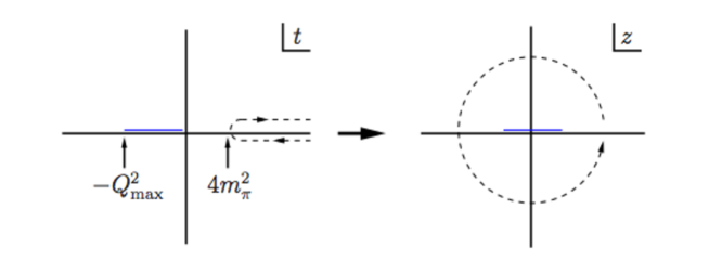
So we begin our model-independent approach by performing a conformal mapping of the domain of analyticity onto the unit circle by defining the variable $z$ as

$$z(t,t_{\rm cut},{t_{0}})=\frac{\sqrt{t_{\rm cut}-t}-\sqrt{t_{\rm cut}-t_{0}}}{\sqrt{t_{\rm cut}-{t}}+\sqrt{t_{\rm cut}-t_{0}}}$$ (5)

where for the present case $t_{\rm cut}$= $4m_{\pi}^{2}$ and ${t_{0}}$ is a free parameter representing the point mapping onto $z$ = 0 .

Since the values of the form factors at $q^{2}=0$ are known, it is convenient to use $t_{0}=0$. The results are independent of this choice [1]. The form factors can be expanded in a power series in $z(q^{2})$:

$$G(q^{2})=\sum_{k=0}^{\infty}a_{k}\,z(q^{2})^{k},$$ (6)

where $z(q^{2})=z(q^{2},t_{\rm cut},t_{0}=0)$.

2.3 Coefficients

The analytic structure in the $t$-plane, illustrated in the Fig.1 implies the dispersion relation,

$$G(t)=\frac{1}{\pi}\int_{t_{\rm cut}}^{\infty}dt^{\prime}\frac{\mbox{Im}G(t^{\prime}+i0)}{t^{\prime}-t}$$ (7)

Equation (5) maps points just above (below) the cut in the $t$ plane onto points in the lower (upper) half unit circle in the z plane . Parameterizing the unit circle by $z(t)$ = $e^{i\theta}$ and solving (5) for $t$ with changed limits we find

$$a_{0} = \frac{1}{\pi}\int_{0}^{\pi}d\theta\,{\rm Re}\,G[t(\theta)+i0]=G(t_{0})\,,$$

$$a_{k} = \frac{2}{\pi}\int_{t_{\rm cut}}^{\infty}\frac{dt}{t-t_{0}}\sqrt{\frac{t_{\rm cut}-t_{0}}{t-t_{\rm cut}}}\mbox{Im}G[t(\theta)+i0]\sin((k\theta(t)),\ k\geq 1$$ (8)

Knowledge of the imaginary part of $G(t)$ helps us put constraints on the coefficients $a_{k}$.

2.4 Bounds on the coefficients

For a realistic extraction of the proton magnetic radius we need to put appropriate bounds on the coefficients $a_{k}$. In [1] Hill and Paz showed that in order to extract the electric charge radius $r_{E}^{p}$ the bounds $|a_{k}|\leq 5,10$ are conservative enough.

The vector dominance ansatz [8] was used to estimate the size of the $a_{k}$. Also from eqn.(3) the magnetic form factors at $q^{2}=0$ are given by $G_{M}^{(0)}(0)\approx 0.88$ and $G_{M}^{(1)}(0)\approx 4.7$, compared to $G_{E}^{(0,1)}(0)=1$. Since the vector dominance ansatz is normalized by the value at $q^{2}=0$, coefficients are proportional to this value. Thus we find that $|a_{k}|\leq 1.1$ for $I=0$ and $|a_{k}|\leq 5.1$ for $I=1$.

Since for the magnetic isovector form factor the singularities that are closest to the cut arise from the two pion continuum we used explicit $\pi\pi$ continuum to find $a_{0}\approx 7.9$, $a_{1}\approx-5.5$, $a_{2}\approx-6.1$, $a_{3}\approx-2.9$, $a_{4}\approx 1.1$ [8]. Also for the case of two nucleon threshold we used $e^{+}e^{-}\to N\bar{N}$ data to constrain the magnetic form factor. Calculations using these data showed that the contribution to $|a_{k}|$ in the region $t\geq 4m_{N}^{2}$ can be neglected [8]. Therefore we conclude that $|a_{k}|\leq 5$ is too stringent and we use the looser bounds $|a_{k}|\leq 10$ and $|a_{k}|\leq 15$ as our default.

One can also use a bound on the ratio $|\frac{a_{k}}{a_{0}}|$ [8]. From the known value of $a_{0}$ this translates to a bound on $|a_{k}|$. In [8] it was shown that the results from bounds on the ratio are consistent with the values extracted using the default bounds. The same is true for a higher bound like $|a_{k}|\leq 20$.

3 Proton magnetic radius extraction

3.1 Proton data

For our data fitting we use (6). We fit our data by minimizing a $\chi^{2}$ function [1] ,

$$\chi^{2}=\sum_{i}(\mbox{data}_{\,i}-\mbox{theory}_{i})^{2}/(\sigma_{i})^{2},$$ (9)

Where $i$ ranges over the tabulated values of [11] up to a given maximal value of $Q^{2}$, with $Q^{2}=0.1,0.2,\dots,1.2,1.4,1.6,1.8$ GeV².

We chose our default bounds on the coefficients to be $|a_{k}|\leq 10,15$. The magnetic radius is then found by using eqn.(4). The extracted values are found to be independent of the number of coefficients we fit. Our default is 8 parameters. We present results in the Table 1 and 2 for two specific ranges of $Q^{2}\leq 0.5$ GeV² and $Q^{2}\leq 1.0$ GeV².

Bound on $a_{k}$	$r_{M}^{p}$	$+\sigma$	$-\sigma$
5	0.89	0.03	0.05
10	0.91	0.03	0.06
15	0.92	0.04	0.07
20	0.93	0.04	0.07

Table 1: $Q^{2}\leq 0.5$ GeV²

Bound on $a_{k}$	$r_{M}^{p}$	$+\sigma$	$-\sigma$
5	0.89	0.02	0.05
10	0.91	0.03	0.07
15	0.91	0.04	0.07
20	0.91	0.05	0.08

Table 2: $Q^{2}\leq 1.0$ GeV²

3.2 Proton and neutron data

Inclusion of the neutron data helps us to separate the isoscalar ($I=0$) and isovector ($I=1$) components of the proton form factor. For the neutron form factors ($G_{M}^{n}$) we use the data tabulated in [12, 13, 14, 15, 16, 17, 18].

Again we observed that the central values of the extracted proton magnetic radius is consistent and do not depend on the number of coefficients we fit [8] as shown in Table 3 and Table 4.

Bound on $a_{k}$	$r_{M}^{p}$	$+\sigma$	$-\sigma$
5	0.86	0.02	0.01
10	0.87	0.04	0.05
15	0.87	0.05	0.05
20	0.88	0.04	0.06

Table 3: $Q^{2}\leq 0.5$ GeV²

Bound on $a_{k}$	$r_{M}^{p}$	$+\sigma$	$-\sigma$
5	0.87	0.02	0.02
10	0.88	0.02	0.05
15	0.88	0.04	0.05
20	0.88	0.05	0.06

Table 4: $Q^{2}\leq 1.0$ GeV²

3.3 Proton, neutron and $\pi\pi$ data

Between the two-pion and four-pion threshold the only state that can contribute to the imaginary part of the magnetic isovector form factor is that of two pions. We can use the known information about ${\rm Im}\,G_{M}^{(1)}(t)$ in this region to raise the effective threshold of isovector form factor from $t_{\rm cut}=4m_{\pi}^{2}$ to $t_{\rm cut}=16m_{\pi}^{2}$. The fitting is done by [1]

$$G_{M}^{(1)}(t)=G_{\rm cut}(t)+\sum_{k}a^{(1)}_{k}z^{k}(t,t_{\rm cut}=16m_{\pi}^{2},0).$$ (10)

$G_{\rm cut}(t)$ is calculated from eqn.(7). Again, the extracted values are independent of the number of fitting parameters and are consistent over the range of $Q^{2}$. The error bars are also smaller. The results are presented in Tables 5 and 6.

Bound on $a_{k}$	$r_{M}^{p}$	$+\sigma$	$-\sigma$
5	0.867	0.010	0.013
10	0.871	0.011	0.015
15	0.873	0.012	0.016
20	0.876	0.012	0.018

Table 5: $Q^{2}\leq 0.5$ GeV²

Bound on $a_{k}$	$r_{M}^{p}$	$+\sigma$	$-\sigma$
5	0.867	0.006	0.008
10	0.874	0.008	0.015
15	0.874	0.012	0.014
20	0.875	0.013	0.016

Table 6: $Q^{2}\leq 1.0$ GeV²

4 Neutron magnetic radius extraction

The magnetic radius of the neutron is defined as $r_{M}^{n}\equiv\sqrt{\langle r^{2}\rangle_{M}^{n}}$, where

$$\langle r^{2}\rangle_{M}^{n}=\frac{6}{G_{M}^{n}(0)}\frac{d}{dq^{2}}G_{M}^{n}(q^{2})\bigg{|}_{q^{2}=0}\,.$$ (11)

We used the same technique and same data sets to extract the magnetic radius of neutron. Some results are shown in Table 7.

$Q^{2}$(GeV²) Bound on $a_{k}$ Neutron data Neutron and Proton data Neutron,Proton and $\pi\pi$ data $r_{M}^{n}$ $+\sigma$ $-\sigma$ $r_{M}^{n}$ $+\sigma$ $-\sigma$ $r_{M}^{n}$ $+\sigma$ $-\sigma$ 0.5 10 0.74 0.13 0.06 0.89 0.06 0.09 0.89 0.03 0.03 15 0.65 0.21 0.07 0.88 0.08 0.09 0.89 0.03 0.03 1.0 10 0.77 0.17 0.09 0.88 0.06 0.08 0.88 0.03 0.01 15 0.74 0.20 0.11 0.89 0.07 0.10 0.88 0.03 0.02

Table 7: Neutron magnetic radii for different data sets

5 Conclusion

The purpose of this analysis was to try to resolve the discrepancies that exist in the literature regarding the extraction of the magnetic radius of the proton. To achieve that we used the “$z$-expansion” method which incorporates the analytic structure of the form factors.

Three data sets have been used for the extraction. From the proton data set we extracted the magnetic radius of the proton as $r_{M}^{p}=0.91_{-0.06}^{+0.03}\pm 0.02$ fm. Inclusion of the neutron data gives the radius $r_{M}^{p}=0.87_{-0.05}^{+0.04}\pm 0.01$ fm. When we add the $\pi\pi$ data along with these data sets the extracted value of the magnetic radius is $r_{M}^{p}=0.87_{-0.02}^{+0.02}$ fm. Comparing our results with the PDG value $r_{M}^{p}=0.777\pm 0.014$ fm [4] we can say that our results are more consistent with the results of $r_{M}^{p}=0.854\pm 0.005$ fm extracted in [6] or $r_{M}^{p}=0.876\pm 0.020$ fm [7] . Our study has also revealed that the extracted magnetic radius is independent of the number of parameters we fit or the range of $Q^{2}$ we used. We have reported all our results with 8 parameters and two specific ranges $Q^{2}\leq 0.5$ GeV² and $Q^{2}\leq 1.0$ GeV².

The same procedure was applied to extract the magnetic radius of the neutron. Combining all three data sets (neutron, proton and $\pi\pi$) we extract the radius of the neutron to be $r_{M}^{n}=0.89\pm 0.03$ fm. Interestingly we notice that within the errors this value is consistent with the magnetic radius of the proton $r_{M}^{p}=0.87\pm 0.02$ fm.

Acknowledgements This work was supported by DOE grant DE-SC0007983.

References

- [1] R. J. Hill and G. Paz, Phys. Rev. D 82, 113005 (2010) [arXiv:1008.4619 [hep-ph]].
- [2] R. Pohl et al., Nature 466, 213 (2010).
- [3] A. Antognini, F. Nez, K. Schuhmann, F. D. Amaro, FrancoisBiraben, J. M. R. Cardoso, D. S. Covita and A. Dax et al., Science 339, 417 (2013).
- [4] K.A. Olive et al. (Particle Data Group), Chin. Phys. C, 38, 090001 (2014)
- [5] J. C. Bernauer et al. [A1 Collaboration], Phys. Rev. Lett. 105, 242001 (2010) [arXiv:1007.5076 [nucl-ex]].
- [6] M. A. Belushkin, H. W. Hammer and U. G. Meissner, Phys. Rev. C 75, 035202 (2007) [arXiv:hep-ph/0608337].
- [7] D. Borisyuk, Nucl. Phys. A 843, 59 (2010) [arXiv:0911.4091 [hep-ph]].
- [8] Z. Epstein, G. Paz and J. Roy, Phys. Rev. D 90, no. 7, 074027 (2014) [arXiv:1407.5683 [hep-ph]].
- [9] F. J. Ernst, R. G. Sachs and K. C. Wali, Phys. Rev. 119, 1105 (1960).
- [10] J. Beringer et al. [Particle Data Group Collaboration], Phys. Rev. D 86, 010001 (2012).
- [11] J. Arrington, W. Melnitchouk and J. A. Tjon, Phys. Rev. C 76, 035205 (2007) [arXiv:0707.1861 [nucl-ex]].
- [12] A. Lung, L. M. Stuart, P. E. Bosted, L. Andivahis, J. Alster, R. G. Arnold, C. C. Chang and F. S. Dietrich et al., Phys. Rev. Lett. 70, 718 (1993).
- [13] H. Gao, J. Arrington, E. J. Beise, B. Bray, R. W. Carr, B. W. Filippone, A. Lung and R. D. McKeown et al., Phys. Rev. C 50, 546 (1994).
- [14] H. Anklin, D. Fritschi, J. Jourdan, M. Loppacher, G. Masson, I. Sick, E. E. W. Bruins and F. C. P. Joosse et al., Phys. Lett. B 336, 313 (1994).
- [15] H. Anklin, L. J. deBever, K. I. Blomqvist, W. U. Boeglin, R. Bohm, M. Distler, R. Edelhoff and J. Friedrich et al., Phys. Lett. B 428, 248 (1998).
- [16] G. Kubon, H. Anklin, P. Bartsch, D. Baumann, W. U. Boeglin, K. Bohinc, R. Bohm and M. O. Distler et al., Phys. Lett. B 524, 26 (2002) [nucl-ex/0107016].
- [17] B. Anderson et al. [Jefferson Lab E95-001 Collaboration], Phys. Rev. C 75, 034003 (2007) [nucl-ex/0605006].
- [18] J. Lachniet et al. [CLAS Collaboration], Phys. Rev. Lett. 102, 192001 (2009) [arXiv:0811.1716 [nucl-ex]].