On a Problem of Weighted Low Rank Approximation of Matrices

Abstract

We study a weighted low rank approximation that is inspired by a problem of constrained low rank approximation of matrices as initiated by the work of Golub, Hoffman, and Stewart (Linear Algebra and Its Applications, 88-89(1987), 317-327). Our results reduce to that of Golub, Hoffman, and Stewart in the limiting cases. We also propose an algorithm based on the alternating direction method to solve our weighted low rank approximation problem and compare it with the state-of-art general algorithms such as the weighted total alternating least squares and the EM algorithm.

1 Introduction

Let $m$ and $n$ be two natural numbers. For an integer $r\leq\min\{m,n\}$ and a matrix $A\in\mathbb{R}^{m\times n}$, the standard low rank approximation problem can be formulated as

(1) $$\min_{\begin{subarray}{c}{X}\in\mathbb{R}^{m\times n}\\ {\rm r}({X})\leq r\end{subarray}}\|A-{X}\|_{F}^{2},$$

where ${\rm r}({X})$ denotes the rank of the matrix ${X}$ and $\|\cdot\|_{F}$ denotes the Frobenius norm of matrices.

It is well known that the solutions to this problem can be given using the singular value decompositions (SVDs) of $A$ through the hard thresholding operations on the singular values: The solutions to (1) are given by

(2) $$X^{*}=H_{r}(A):=U(A)\Sigma_{r}(A)V(A)^{T},$$

where $A=U(A)\Sigma(A)V(A)^{T}$ is a SVD of $A$ and $\Sigma_{r}(A)$ is the diagonal matrix obtained from $\Sigma(A)$ by thresholding: keeping only $r$ largest singular values and replacing other singular values by 0 along the diagonal. This is also referred to as Eckart-Young-Mirsky’s theorem ([8]) and is closely related to the PCA method in statistics [4]. The solutions to (1) as given in (2) suffer from the fact that none of the entries of $X$ is guaranteed to be preserved in $X^{*}$. In many real world problems, one has good reasons to keep certain entries of $A$ unchanged while looking for a low rank approximation. In 1987, Golub, Hoffman, and Stewart were the first to consider the following constrained low rank approximation problem [1]:

Given $A=(A_{1}\;\;A_{2})\in\mathbb{R}^{m\times n}$ with $A_{1}\in\mathbb{R}^{m\times k}$ and $A_{2}\in\mathbb{R}^{m\times(n-k)}$, find $\tilde{A}_{2}$ such that (with $\tilde{A}_{1}=A_{1}$)

(3) $$(\tilde{A}_{1}\;\tilde{A}_{2})=\arg\min_{\begin{subarray}{c}X_{1},X_{2}\\ {\rm r}(X_{1}\;\;X_{2})\leq r\\ X_{1}=A_{1}\end{subarray}}\|(A_{1}\;\;A_{2})-(X_{1}\;\;{X}_{2})\|_{F}^{2}.$$

That is, Golub, Hoffman, and Stewart required that certain columns, $A_{1},$ of $A$ must be preserved when one looks for a low rank approximation of $(A_{1}\;\;A_{2}).$ As in the standard low rank approximation, the constrained low rank approximation problem of Golub, Hoffman, and Stewart also has a closed form solution.

Theorem 1.

[1] With $k={\rm r}(A_{1})$ and $r\geq k$, the solutions $\tilde{A}_{2}$ in (3) are given by

(4) $$\tilde{A_{2}}=P_{A_{1}}(A_{2})+H_{r-k}\left(P^{\perp}_{A_{1}}(A_{2})\right),$$

where $P_{A_{1}}$ and $P^{\perp}_{A_{1}}$ are the projection operators to the column space of $A_{1}$ and its orthogonal complement, respectively.

Remark 2.

According to Section 3 of [1], the matrix $\tilde{A}_{2}$ is unique if and only if $H_{r-k}\left(P^{\perp}_{A_{1}}(A_{2})\right)$ is unique, which means the $(r-k)$th singular value of $P^{\perp}_{A_{1}}(A_{2})$ is strictly greater than $(r-k+1)$th singular value. When $\tilde{A}_{2}$ is not unique, the formula for $\tilde{A}_{2}$ given in Theorem 1 should be understood as the membership of the set specified by the right-hand side of (4). We will use this convention in this paper.

Inspired by Theorem 1 above and motivated by applications in which $A_{1}$ may contain noise, it makes more sense if we require $\|A_{1}-X_{1}\|_{F}$ small instead of asking for $X_{1}=A_{1}$. This leads us to consider the following problem: Let $\eta>0$, find $(\hat{X}_{1}\;\;\hat{X}_{2})$ such that

(5) $$(\hat{X}_{1}\;\;\hat{X}_{2})=\arg\min_{\begin{subarray}{c}X_{1},X_{2}:\|A_{1}-X_{1}\|_{F}\leq\eta\\ {\rm r}(X_{1}\;\;X_{2})\leq r\end{subarray}}\|(A_{1}\;\;A_{2})-({X}_{1}\;\;{X}_{2})\|_{F}^{2}.$$

Or, for a large parameter $\lambda$, consider

(6) $$(\hat{X}_{1}\;\;\hat{X}_{2})=\arg\min_{\begin{subarray}{c}X_{1},X_{2}\\ {\rm r}(X_{1}\;\;X_{2})\leq r\end{subarray}}\left\{\lambda^{2}\|A_{1}-X_{1}\|_{F}^{2}+\|A_{2}-{X}_{2}\|_{F}^{2}\right\}.$$

This block structure in weight matrix, where very few entries are heavily weighted and most entries stays at 1 (unweighted), is realistic in applications. For example, in the problem of background estimation in a video sequence, each frame is a column in the data matrix and the background is a low rank (ideally of rank 1) component of the data matrix. So, the weight is used to single out which columns are more likely to be the basis of background frames and the low rank constraint enforces the search for other frames that are in the background subspace. Recent investigations in [2, 3, 7] have shown that the above “approximately” preserving (controlled by a parameter $\lambda$) weighted low rank approximation can be more effective in solving the background modeling, shadows and specularities removal, and domain adaptation problems in computer vision and machine learning.

As it turns out, (6) can be viewed as a generalized total least squares problem (GTLS) and can be solved in closed form as a special case of weighted low rank approximation with a rank-one weight matrix by using a SVD of the given matrix $(\lambda A_{1}\;\;A_{2})$ [21, 22]. As a consequence of the closed form solutions, one can verify that the solution to (3) is the limit case of the solutions to (6) as $\lambda\to\infty$. Thus, (3) can be viewed as a special case when “$\lambda=\infty$”. A careful reader may also note that, problem (6) can be cast as a special case of structured low rank problems with element-wise weights [24, 29]. More specifically, we observe that (6) is contained in the following more general point-wise weighted low rank approximation problem:

(7) $$\min_{\begin{subarray}{c}X_{1},X_{2}\\ {\rm r}(X_{1}\;\;X_{2})\leq r\end{subarray}}\|\left((A_{1}\;\;A_{2})-({X}_{1}\;\;{X}_{2})\right)\odot(W_{1}\;~{}W_{2})\|_{F}^{2},$$

for $W_{1}=\lambda\mathbbm{1}$ and $W_{2}=\mathbbm{1}$ (a matrix whose entries are equal to 1), where $W\in\mathbb{R}^{m\times n}$ is a weight matrix and $\odot$ denotes the Hadamard product.

This is the weighted low rank approximation problem studied first when $W$ is an indicator weight for dealing with the missing data case ([13, 14]) and then for more general weight in machine learning, collaborative filtering, 2-D filter design, and computer vision [9, 15, 19, 26, 27, 28]. For example, if SVD is used in quadrantally-symmetric two-dimensional (2-D) filter design, as explained in [26] (see also [27, 28]), it might lead to a degraded construction in some cases as it is not able to discriminate between the important and unimportant components of $X$. To address this problem, a weighted least squares matrix decomposition method was first proposed by Shpak [28]. Following his idea of assigning different weights to discriminate between important and unimportant components of the test matrix, Lu, Pei, and Wang ([27]) designed a numerical procedure to solve (7) for general weight $(W_{1}\;~{}W_{2})$.

Remark 3.

There is another formulation of weighted low rank approximation problem defined as in [26]:

(8) $$\min_{\begin{subarray}{c}{X}\in\mathbb{R}^{m\times n}\end{subarray}}\|A-X\|_{Q}^{2},~{}~{}{\rm subject~{}to~{}}{\rm r}({X})\leq r,$$

where $Q\in\mathbb{R}^{mn\times mn}$ is a symmetric positive definite weight matrix. Denote $\|A-X\|_{Q}^{2}:={\rm vec}(A-X)^{T}Q{\rm vec}(A-X)$, where ${\rm vec}(\cdot)$ is an operator which maps the entries of $\mathbb{R}^{m\times n}$ to $\mathbb{R}^{mn\times 1}$. It is easy to see that (7) is a special case of (8) with a diagonal $Q$. In this paper, we will not use this more general formulation for simplicity.

Motivated by the limit behavior of (6) as $\lambda\to\infty$, we are interested in finding out the limit behavior of the solutions to problem (7) for general weight $(W_{1}\;~{}W_{2})$ when $(W_{1})_{ij}\to\infty$ and $W_{2}\to\mathbbm{1}$. One can expect that, with appropriate conditions, the limit should be the solutions to (3). We will verify this with an stronger result with estimation on the rate of convergence (when $W_{2}=\mathbbm{1}$). The main challenge here is the lack of closed form solutions to problem (7) in general [9, 26]. We will also extend the convergence result to the unconstrained version of the problem (7).

In order to make use of the proposed weighted low rank approximation in applications, we will propose a numerical algorithm to solve (7) for the special case when $W_{2}=\mathbbm{1}$. In view of the existing algorithms for solving the general weighted low rank approximation problem, we want to emphasize that our special algorithm takes advantage of the block structure of our weights that results in better numerical performance as well as the fact that we have detailed convergence analysis for the algorithm.

The rest of the paper is organized as follows. In Section 2, we state our main results on the behavior of the solutions to (7) as $(W_{1})_{i,j}\to\infty$ and $(W_{2})_{i,j}\to 1$. Their proofs are given in Section 3. In Section 4, we present a numerical solution to problem (7) when $W_{2}=\mathbbm{1}$ and discuss the convergence of our algorithm. Numerical results verifying our main results are given in Section 5.

The extension of our rate of convergence and numerical algorithm to the more general case when $W_{2}=\mathbbm{1}$ is replaced by $W_{2}\to\mathbbm{1}$ is non-trivial and remains open.

2 Limiting behavior of solutions as $(W_{1})_{i,j}\to\infty$ and $(W_{2})_{i,j}\to 1$

Denote $\mathcal{A}=P_{A_{1}}^{\perp}(A_{2})$ and $\tilde{\mathcal{A}}=P_{\tilde{X}_{1}(W)}^{\perp}(A_{2}).$ Also denote $s={\rm r}(\mathcal{A})$ and let the ordered non-zero singular values of $\mathcal{A}$ be $\sigma_{1}\geq\sigma_{2}\geq\cdots\geq\sigma_{s}>0.$ Let $(\tilde{X}_{1}(W)\;~{}\tilde{X}_{2}(W))$ be a solution to (7). Let $\lambda_{j}=\displaystyle{\min_{1\leq i\leq m}(W_{1})_{ij}}$ and $\lambda=\displaystyle{\min_{1\leq j\leq k}\lambda_{j}}$.

Theorem 4.

Suppose that $\sigma_{r-k}>\sigma_{r-k+1}$. Then we have, as $\lambda\to\infty$ and $W_{2}=\mathbbm{1}$,

$$(\tilde{X}_{1}(W)\;\;\tilde{X}_{2}(W))=A_{G}+\displaystyle{O(\frac{1}{\lambda})},$$

where $A_{G}=(A_{1}\;\tilde{A}_{2})$ is defined to be the unique solution to (3).

Remark 5.

(i) The assertion of the uniqueness of $A_{G}$ is due to the assumption $\sigma_{r-k}>\sigma_{r-k+1}$ (see the Remark 2). (ii) The convergence $(\tilde{X}_{1}(W)\;\;\tilde{X}_{2}(W))\to A_{G}$ alone is indeed implied by a general result in [24].

Next, if we do not know $r$ but still want to reduce the rank in our approximation, then we can consider the unconstrained version of (7): for $\tau>0$,

(9) $$\min_{\begin{subarray}{c}X_{1},X_{2}\end{subarray}}\left\{\|\left((A_{1}\;\;A_{2})-({X}_{1}\;\;{X}_{2})\right)\odot(W_{1}\;\;W_{2})\|_{F}^{2}+\tau{\rm r}({X}_{1}\;\;{X}_{2})\right\}.$$

Again, one can expect that the solutions to (9) will converge to the solution of (3) as $(W_{1})_{ij}\to\infty$ and $(W_{2})_{ij}\to 1$. We will first establish a convergence result for (9) without assuming the uniqueness of the solutions to (3).

Let ${\cal A}_{G}^{r}$ be the set of all solutions to (3) and let $(\hat{X}_{1}(W)\;~{}\hat{X}_{2}(W))$ be a solution to (9).

Theorem 6.

Every accumulation point of $(\hat{X}_{1}(W)\;~{}\hat{X}_{2}(W))$ as $(W_{1})_{ij}\to\infty,(W_{2})_{ij}\to 1$ belongs to $\displaystyle{\mathop{\cup}_{0\leq r\leq\min\{m,n\}}{\cal A}_{G}^{r}}.$

Next, we have more precise information of the convergence if we assume the uniqueness of (3).

Theorem 7.

Assume that $\sigma_{1}>\sigma_{2}>\cdots>\sigma_{s}>0$. Denote $\sigma_{0}:=\infty$ and $\sigma_{s+1}:=0.$ Then the accumulation point of the sequence $(\hat{X}_{1}(W)\;\hat{X}_{2}(W)),$ as $(W_{1})_{ij}\to\infty$ and $(W_{2})_{ij}\to 1$ is unique; and this unique accumulation point is given by

$$\left(A_{1}\;\;\;\;P_{A_{1}}(A_{2})+H_{r^{*}}\left(P^{\perp}_{A_{1}}(A_{2})\right)\right)$$

with $r^{*}$ satisfying

$$\sigma_{r^{*}+1}^{2}\leq\tau<\sigma_{r^{*}}^{2}.$$

Remark 8.

For the case when $P^{\perp}_{A_{1}}(A_{2})$ has repeated singular values, we leave it to the reader to verify the following more general statement by using a similar argument: Let $\hat{\sigma}_{1}>\hat{\sigma}_{2}>...>\hat{\sigma}_{t}>0$ be the singular values of $P^{\perp}_{A_{1}}(A_{2})$ with multiplicity $k_{1},k_{2},\cdots k_{t}$ respectively. Note that $\sum_{i=1}^{t}k_{i}=s.$ Let $\sigma_{p^{*}+1}^{2}\leq\tau<\sigma_{p^{*}}^{2},$ where $\sigma_{p^{*}}$ has multiplicity $k_{p^{*}}.$ Then the accumulation points of the set $(\hat{X}_{1}(W)\;~{}\hat{X}_{2}(W)),$ as $(W_{1})_{ij}\to\infty,(W_{2})_{ij}\to 1$, belongs to the set $\displaystyle{\mathop{\cup}_{r^{*}}{\cal A}_{G}^{r^{*}}},$ where $1+\sum_{i=1}^{p^{*}-1}k_{i}\leq r^{*}<\sum_{i=1}^{p^{*}}k_{i}.$

3 Proofs of results in Section 2

To prove Theorem 4, we start with a few well known results from the perturbation theory of singular values. First, we quote the following result of Stewart.

Lemma 9.

[10] Let $\tilde{{A}}={{A}}+E$ and $\sigma\neq 0$ be a non-repeating singular value of the matrix ${A}$ with $u$ and $v$ being left and right singular vectors respectively. Then as $\|E\|\to 0,$ there is a unique singular value $\tilde{\sigma}$ of $\tilde{{A}}$ such that

(10) $$\tilde{\sigma}=\sigma+u^{T}Ev+O(\|E\|^{2}).$$

Let the SVDs of ${B},~{}\tilde{{B}}\in\mathbb{R}^{m\times n}$ be given by

(11) $${B}=U\Sigma V^{T}=(U_{1}\;U_{2})\begin{pmatrix}\Sigma_{1}&0\\ 0&\Sigma_{2}\\ \end{pmatrix}\begin{pmatrix}V_{1}^{T}\\ V_{2}^{T}\end{pmatrix}=:{B}_{1}+{B}_{2},$$

(12) $$\tilde{{B}}=\tilde{U}\tilde{\Sigma}\tilde{V}^{T}=(\tilde{U}_{1}\;\tilde{U}_{2})\begin{pmatrix}\tilde{\Sigma}_{1}&0\\ 0&\tilde{\Sigma}_{2}\\ \end{pmatrix}\begin{pmatrix}\tilde{V}_{1}^{T}\\ \tilde{V}_{2}^{T}\end{pmatrix}=:\tilde{{B}}_{1}+\tilde{{B}}_{2},$$

such that $U,~{}\tilde{U}\in\mathbb{R}^{m\times m},~{}V,~{}\tilde{V}\in\mathbb{R}^{n\times n},\;\text{and}\;~{}\Sigma,~{}\tilde{\Sigma}\in\mathbb{R}^{m\times n}$ with $\Sigma$ and $\tilde{\Sigma}$ being diagonal matrices containing singular values of ${B}$ and $\tilde{{B}}$, respectively, arranged in a non-increasing order; $U_{1},~{}\tilde{U}_{1}\in\mathbb{R}^{m\times s},U_{2},~{}\tilde{U}_{2}\in\mathbb{R}^{m\times(m-s)},V_{1},~{}\tilde{V}_{1}\in\mathbb{R}^{n\times s},\;\text{and}\;~{}V_{2},~{}\tilde{V}_{2}\in\mathbb{R}^{n\times(n-s)}.$ Using (11) and (12) we have, with $E=\tilde{B}-B$,

(13) $$\tilde{{B}}_{1}+\tilde{{B}}_{2}=\tilde{{B}}={B}+E={B}_{1}+{B}_{2}+E.$$

Next, we state a special form of the sin$\theta$ Theorem of Wedin (see [32, p. 260] and [6]) as follows.

Lemma 10.

With the notations above, let $\eta=\sigma_{min}(\tilde{B}_{1})-\sigma_{max}({B}_{2})>0$. Then

$$\sqrt{\|\sin\Theta(U_{1},\tilde{U}_{1})\|^{2}_{F}+\|\sin\Theta(V_{1},\tilde{V}_{1})\|^{2}_{F}}\leq\frac{\sqrt{2}\|E\|_{F}}{\eta}.$$

Finally, using the argument of Wedin ([6]), the following result can be achieved.

Lemma 11.

([6, Sect. 4.4]). Assume there exists an $\alpha\geq 0$ and a $\delta>0$ such that

$$\sigma_{min}(\tilde{{B}}_{1})\geq\alpha+\delta\;\;\text{and}\;\;\sigma_{max}({B}_{2})\leq\alpha,$$

then

(14) $$\|{B}_{1}-\tilde{{B}}_{1}\|\leq\|E\|(3+\frac{\|{B}_{2}\|}{\delta}+\frac{\|\tilde{{B}}_{2}\|}{\delta}).$$

Now, we establish some auxiliary results. Let $P_{B}$ and $P_{\tilde{B}}$ be the orthogonal projections onto the column spaces of matrices $B$ and $\tilde{B}$, respectively.

Lemma 12.

Assume that $B$ and $\tilde{B}$ are full rank matrices. Let $\eta$ denote the smallest singular value of $\tilde{B}$. Then

(15) $$\|P_{B}-P_{\tilde{B}}\|_{F}\leq\frac{2\|B-\tilde{B}\|_{F}}{\eta}.$$

Proof.

According to [32, p. 43], we have

(16) $$\|P_{B}-P_{\tilde{B}}\|_{F}=\sqrt{2}\|\sin\Theta(B,\tilde{B})\|_{F},$$

where $\Theta(B,\tilde{B})$ is the canonical angle (diagonal) matrix between the column spaces of $B$ and $\tilde{B}$. Now, by applying Lemma 10 to the case when $U_{2}=\tilde{U}_{2}=\emptyset$ (so that $U_{1}$ and $\tilde{U}_{1}$ span the same column spaces as those of $B$ and $\tilde{B}$, respectively, and so $\Theta(B,\tilde{B})=\Theta(U_{1},\tilde{U}_{1})$ with $\eta=\sigma_{min}(\tilde{B}_{1})>0$ (since $\sigma({B}_{2})=0$), we have

(17) $$\|\sin\Theta(B,\tilde{B})\|_{F}=\|\sin\Theta(U_{1},\tilde{U}_{1})\|_{F}\leq\frac{\sqrt{2}\|B-\tilde{B}\|_{F}}{\eta}.$$

Now, the inequality (15) follows from (16) and (17). ∎

Lemma 13.

As $(W_{1})_{ij}\to\infty$ and $W_{2}$ stays bounded, we have the following estimates.

1. $\tilde{X}_{1}(W)=A_{1}+\displaystyle{O(\frac{1}{\lambda})}$.

2. $P_{\tilde{X}_{1}(W)}(A_{2})=P_{A_{1}}(A_{2})+\displaystyle{O(\frac{1}{\lambda})}$.

3. $P_{\tilde{X}_{1}(W)}^{\perp}(A_{2})=P_{A_{1}}^{\perp}(A_{2})+\displaystyle{O(\frac{1}{\lambda})}$.

Proof.

(i). Note that,

$$\|(A_{1}-\tilde{X}_{1}(W))\odot W_{1}\|_{F}^{2}+\|(A_{2}-\tilde{X}_{2}(W))\odot W_{2}\|_{F}^{2}$$

$$=\min_{\begin{subarray}{c}{X}_{1},{X}_{2}\\ {\rm r}({X}_{1}\;\;{X}_{2})\leq r\end{subarray}}\left(\|(A_{1}-{X}_{1})\odot W_{1}\|_{F}^{2}+\|(A_{2}-{X}_{2})\odot W_{2}\|_{F}^{2}\right)$$

$$\leq\|A_{2}\odot W_{2}\|_{F}^{2}\;(\text{by taking}\;(X_{1}\;\;X_{2})=(A_{1}\;\;0)).$$

Then $\displaystyle{\sum_{\begin{subarray}{c}1\leq i\leq m\\ 1\leq j\leq k\end{subarray}}((A_{1})_{ij}-(\tilde{X}_{1}(W))_{ij})^{2}(W_{1})_{ij}^{2}\leq\|A_{2}\odot W_{2}\|_{F}^{2}}$ and so

$$|(A_{1})_{ij}-(\tilde{X}_{1}(W))_{ij}|\leq\frac{\|A_{2}\odot W_{2}\|_{F}}{(W_{1})_{ij}};~{}~{}1\leq i\leq m,1\leq j\leq k.$$

Thus

$$\tilde{X}_{1}(W)=A_{1}+\displaystyle{O(\frac{1}{\lambda})}\;\text{as}\;\lambda\to\infty.$$

(ii). Note that as $\lambda\to\infty$, $\tilde{X}_{1}(W)\to A_{1}$. So, $\tilde{X}_{1}(W)$ will be a full rank matrix (since $A_{1}$ is assumed to be of full rank). Applying (i) and Lemma 15 to $B=A_{1}$ and $\tilde{B}=\tilde{X}_{1}(W)$, we have, as $\lambda\to\infty$,

$$\|P_{A_{1}}-P_{\tilde{X}_{1}(W)}\|_{F}\leq\frac{2}{\eta(\tilde{X}_{1}(W))}O(\frac{1}{\lambda}).$$

Since $\eta(\tilde{X}_{1}(W))\to\eta(A_{1})>0$, we have $\eta(\tilde{X}_{1}(W))\geq\eta(A_{1})/2$ as $\lambda\to\infty$. Thus, (ii) holds.
(iii) We know that

$$P_{\tilde{X}_{1}(W)}(A_{2})+P_{\tilde{X}_{1}(W)}^{\perp}(A_{2})=A_{2}=P_{A_{1}}(A_{2})+P_{A_{1}}^{\perp}(A_{2}).$$

Using (ii)

$$P_{A_{1}}(A_{2})+\displaystyle{O(\frac{1}{\lambda})}+P_{\tilde{X}_{1}(W)}^{\perp}(A_{2})=P_{A_{1}}(A_{2})+P_{A_{1}}^{\perp}(A_{2}),~{}\lambda\to\infty.$$

Therefore,

(18) $$P_{\tilde{X}_{1}(W)}^{\perp}(A_{2})=P_{A_{1}}^{\perp}(A_{2})+O(\frac{1}{\lambda}),~{}\lambda\to\infty.$$

This completes the proof of Lemma 13.  ∎

Remark 14.

(i) For the case when there is an uniform weight in $(W_{1})_{ij}=\lambda>0$, one might refer to [25] for an alternative proof of Lemma 13. But the proof in [25] can not be applied in the more general weight. (ii) There is a more elementary proof of (ii) of Lemma 13 above by using the Gram-Schmidt process (see [11]), instead of using the advanced tools from the perturbation theory of singular values of Stewart and Wedin. We choose to use the shorter proof here because we need to invoke the advanced theory for the proof of the next lemma anyway.

Next, we establish a key lemma on the hard thresholding operator under perturbation. We use the notation introduced at the beginning of Section 2.

Lemma 15.

Let $W_{2}$ be bounded. If $\sigma_{r-k}>\sigma_{r-k+1},$ then

(19) $$H_{r-k}(\tilde{\mathcal{A}})=H_{r-k}(\mathcal{A})+\displaystyle{O(\frac{1}{\lambda})},~{}\lambda\to\infty.$$

Proof.

Apply (11) and (12) with $B=\mathcal{A}$ and $\tilde{B}=\tilde{\mathcal{A}}$. Then by (iii) of Lemma 13, we know that $E=\tilde{\mathcal{A}}-{\mathcal{A}}=O(\frac{1}{\lambda}).$ Indeed, with the non-increasing arrangement of the singular values in $\Sigma$ and $\tilde{\Sigma}$, and the fact that $E=\displaystyle{O(\frac{1}{\lambda})}$ as $\lambda\to\infty$, Lemma 9 immediately implies that

(20) $$\Sigma_{1}-\tilde{\Sigma}_{1}=\displaystyle{O(\frac{1}{\lambda})}~{}\;\;\text{and}\;\;\Sigma_{2}-\tilde{\Sigma}_{2}=O(\frac{1}{\lambda})\;\;\text{as}\;\lambda\to\infty.$$

Note that, ${\rm r}(\mathcal{A}_{1})={\rm r}(\tilde{\mathcal{A}}_{1})=r-k,$ and, since $\sigma_{r-k}>\sigma_{r-k+1},$ we can choose $\delta$ such that

$$\delta=\frac{1}{2}(\sigma_{r-k}-\sigma_{r-k+1})>0.$$

In this way, for all large $\lambda$ the assumption of Lemma 11 will be satisfied. Since $\mathcal{A}_{1}=H_{r-k}(\mathcal{A})$ and $\tilde{\mathcal{A}}_{1}=H_{r-k}(\tilde{\mathcal{A}}),$ (14) can be written as

(21) $$\|H_{r-k}(\mathcal{A})-H_{r-k}(\tilde{\mathcal{A}})\|\leq\|E\|(3+\frac{\|\mathcal{A}_{2}\|}{\delta}+\frac{\|\tilde{\mathcal{A}}_{2}\|}{\delta}).$$

Since ${\mathcal{A}_{2}}$ is fixed, $\|{\mathcal{A}_{2}}\|=O(1)$ as $\lambda\to\infty$. On the other hand, by (20), as $\lambda\to\infty$,

$$\tilde{\mathcal{A}_{2}}=\tilde{U}_{2}\tilde{\Sigma}_{2}\tilde{V}_{2}^{T}=\tilde{U}_{2}({\Sigma}_{2}+O(\frac{1}{\lambda}))\tilde{V}_{2}^{T}=\tilde{U}_{2}\Sigma_{2}\tilde{V}_{2}^{T}+O(\frac{1}{\lambda}\tilde{U}_{2}\tilde{V}_{2}^{T}).$$

Now the unitary invariance of the matrix norm implies,

$$\|\tilde{\mathcal{A}_{2}}\|\leq\|\tilde{U}_{2}\Sigma_{2}\tilde{V}_{2}^{T}\|+O(\frac{1}{\lambda}\|\tilde{U}_{2}\tilde{V}_{2}^{T}\|)=\|\Sigma_{2}\|+O(\frac{1}{\lambda}),$$

which is bounded as $\lambda\to\infty$. Therefore (21) becomes

(22) $$\|H_{r-k}(\mathcal{A})-H_{r-k}(\tilde{\mathcal{A}})\|\leq C\|E\|,$$

for some constant $C>0$ and for all large $\lambda\to\infty$. Thus

$$H_{r-k}(\tilde{\mathcal{A}})=H_{r-k}(\mathcal{A})+\displaystyle{O(\frac{1}{\lambda})},\lambda\to\infty,$$

since $E=\displaystyle{O(\frac{1}{\lambda})}$ as $\lambda\to\infty$. This completes the proof of Lemma 15. ∎

Proof of Theorem 4. We first note that, for all $X_{2}$ with $r(\tilde{X}_{1}(W)\;~{}X_{2})\leq r$,

$$\|((A_{1}\;~{}A_{2})-(\tilde{X}_{1}(W)\;~{}\tilde{X}_{2}(W)))\odot(W_{1}\;~{}\mathbbm{1})\|_{F}\leq\|((A_{1}\;~{}A_{2})-(\tilde{X}_{1}(W)\;~{}X_{2}))\odot(W_{1}\;~{}\mathbbm{1})\|_{F}.$$

So, $\tilde{X}_{2}(W)$ solves

$$\|A_{2}-\tilde{X}_{2}(W)\|_{F}=\inf_{X_{2}:r(\tilde{X}_{1}(W)\;~{}X_{2})\leq r}\|A_{2}-X_{2}\|_{F}.$$

Thus, by Theorem 1,

$$\tilde{X}_{2}(W)=P_{\tilde{X}_{1}(W)}(A_{2})+H_{r-k}(P_{\tilde{X}_{1}(W)}^{\perp}(A_{2})).$$

Therefore, using (ii) and (iii) of Lemma 13 and Lemma 15, we get, as $\lambda\to\infty$,

$$\tilde{X}_{2}(W)=P_{A_{1}}(A_{2})+H_{r-k}(P_{A_{1}}^{\perp}(A_{2}))+O(\frac{1}{\lambda})=\tilde{A}_{2}+O(\frac{1}{\lambda}).$$

This, together with (i) of Lemma 13, yields the desired result. $\Box$

Proof of Theorem 6. Let $\hat{X}(W)=(\hat{X}_{1}(W)\;\;\hat{X}_{2}(W))$. We need to verify that $\{\hat{X}(W)\}_{W}$ is a bounded set and every accumulation point (as $(W_{1})_{ij}\to\infty$ and $(W_{2})_{ij}\to 1$) is a solution to (3) for some $r$. Since $(\hat{X}_{1}(W)\;\;\hat{X}_{2}(W))$ is a solution to (9), we have

$$\|(A_{1}-\hat{X}_{1}(W))\odot W_{1}\|_{F}^{2}+\|(A_{2}-\hat{X}_{2}(W))\odot W_{2}\|_{F}^{2}+\tau{\rm r}(\hat{X}_{1}(W)\;\;\hat{X}_{2}(W))$$

(23) $$\leq\|(A_{1}-{X}_{1})\odot W_{1}\|_{F}^{2}+\|(A_{2}-{X}_{2})\odot W_{2}\|_{F}^{2}+\tau{\rm r}({X}_{1}\;\;{X}_{2}).$$

for all $({X}_{1}\;\;{X}_{2}).$ By choosing $X_{1}=A_{1},X_{2}=0$, we can obtain a constant $m_{3}:=\|A_{2}\odot W_{2}\|_{F}^{2}+\tau{\rm r}(A_{1}\;\;0)$ such that $\|(A_{1}-\hat{X}_{1}(W))\odot W_{1}\|_{F}^{2}+\|(A_{2}-\hat{X}_{2}(W))\odot W_{2}\|_{F}^{2}\leq m_{3}.$ Therefore, $\{\hat{X}_{1}(W)\;\;\hat{X}_{2}(W)\}$ is bounded. Let $(X_{1}^{**}\;\;X_{2}^{**})$ be an accumulation point of the sequence for some subsequences as $(W_{1})_{ij}\to\infty$ and $(W_{2})_{ij}\to 1$. We only need to show that $(X_{1}^{**}\;\;X_{2}^{**})\in\displaystyle{\mathop{\cup}_{r}{\cal A}_{G}^{r}}.$ As in the proof of Lemma 13 (i), we can show that

(24) $$\lim_{\begin{subarray}{c}(W_{1})_{ij}\to\infty\\ (W_{2})_{ij}\to 1\end{subarray}}\hat{X}_{1}(W)=A_{1}.$$

Now, taking limit and setting $X_{1}=A_{1}$ in (3), we obtain,

(25) $$\|A_{2}-X_{2}^{**}\|_{F}^{2}+\tau{\rm r}(A_{1}\;\;{X}_{2}^{**})\leq\|A_{2}-{X}_{2}\|_{F}^{2}+\tau{\rm r}(A_{1}\;\;{X}_{2}),$$

for all ${X}_{2}.$ If we denote $r^{**}={\rm r}(A_{1}\;\;{X}_{2}^{**}),$ then for ${X}_{2}$ with ${\rm r}(A_{1}\;\;{X}_{2})\leq r^{**},$ (25) yields

(26) $$\|A_{2}-X_{2}^{**}\|_{F}^{2}\leq\|A_{2}-{X}_{2}\|_{F}^{2}.$$

Therefore, $X_{2}^{**}$ is a solution to the problem of Golub, Hoffman, and Stewart and by Theorem 1,

$$X_{2}^{**}=P_{A_{1}}(A_{2})+H_{r^{**}-k}\left(P^{\perp}_{A_{1}}(A_{2})\right).$$

This, together with (24) completes the proof. $\Box$

Proof of Theorem 7. For convenience, we will drop the dependence on $W$ in our notations. Let $\hat{X}=(\hat{X}_{1}\;\;\hat{X}_{2})$ solve the minimization problem (9). As in the proof of Lemma 13 (i) again we have

(27) $$\hat{X}_{1}\to A_{1},~{}{\rm as}~{}(W_{1})_{ij}\to\infty.$$

Next, we show the convergence of $\hat{X}_{2}$: for $r^{*}$ satisfying $\sigma_{r^{*}}^{2}>\tau\geq\sigma_{r^{*}+1}^{2}$,

(28) $$\hat{X}_{2}\to P_{A_{1}}(A_{2})+H_{r^{*}}(P_{A_{1}}^{\perp}(A_{2})),~{}{\rm as}~{}(W_{1})_{i,j}\to\infty,~{}(W_{2})_{i,j}\to 1.$$

By Theorem 6, $\hat{X}$ is bounded. So, to establish (28), we will need only to show (i) there is only one accumulation point as $(W_{1})_{i,j}\to\infty,~{}(W_{2})_{i,j}\to 1$, and (ii) this unique accumulation point is $P_{A_{1}}(A_{2})+H_{r^{*}}(P_{A_{1}}^{\perp}(A_{2}))$ for $r^{*}$ satisfying $\sigma_{r^{*}}^{2}>\tau\geq\sigma_{r^{*}+1}^{2}$.

Let $X_{2}^{*}$ be any accumulation point of $\hat{X}_{2}$ as $(W_{1})_{i,j}\to\infty,~{}(W_{2})_{i,j}\to 1$.

Choosing $X_{1}=\hat{X}_{1}$ in (3) we find, for all $X_{2}$,

(29) $$\;\;\;\;\;\;\|(A_{2}-\hat{X}_{2})\odot W_{2}\|_{F}^{2}+\tau{\rm r}(\hat{X}_{1}\;\;\hat{X}_{2})\leq\|(A_{2}-{X}_{2})\odot W_{2}\|_{F}^{2}+\tau{\rm r}(\hat{X}_{1}\;\;{X}_{2}).$$

We will apply some ideas from Golub, Hoffman, and Stewart  [1]. Since the weight $W_{2}$ gets in the way (by destroying the unitary invariance of the norm), we have to take the limit $(W_{2})_{i,j}\to 1$ at the right time.

As in [1], assume ${\rm r}(A_{1})=k$ and consider a $QR$ decomposition of $A$ and corresponding decomposition of $\hat{X}$ and $X$:

$$A=QR=(Q_{1}~{}~{}Q_{2})\begin{pmatrix}{R}_{11}&{R}_{12}\\ 0&R_{22}\\ 0&0\end{pmatrix}=(Q_{1}R_{11}~{}~{}Q_{1}R_{12}+Q_{2}\begin{pmatrix}R_{22}\\ 0\end{pmatrix})=(A_{1}~{}~{}A_{2}),$$

let

$$\hat{R}:=Q^{T}\hat{X}=\begin{pmatrix}\hat{R}_{11}&\hat{R}_{12}\\ \hat{R}_{21}&\hat{R}_{22}\\ \hat{R}_{31}&\hat{R}_{32}\end{pmatrix}$$

and let

$${R}^{\dagger}:=Q^{T}X=\begin{pmatrix}{R}^{\dagger}_{11}&{R}^{\dagger}_{12}\\ {R}^{\dagger}_{21}&{R}^{\dagger}_{22}\\ {R}^{\dagger}_{31}&{R}^{\dagger}_{32}\end{pmatrix}.$$

Since the rank of a matrix is invariant under an unitary transformation, (29) can be rewritten as

$$\|(A_{2}-\hat{X}_{2})\odot W_{2}\|_{F}^{2}+\tau{\rm r}(Q^{T}\hat{X}_{1}\;\;Q^{T}\hat{X}_{2})$$

(30) $$\leq\|(A_{2}-{X}_{2})\odot W_{2}\|_{F}^{2}+\tau{\rm r}(Q^{T}\hat{X}_{1}\;\;Q^{T}{X}_{2}).$$

When $\lambda=\min_{i,j}(W_{1})_{i,j}$ is large enough, $\hat{R}_{11}$ is nonsingular by (27). Using ${\rm r}(A_{1})=k$ and performing the row and column operations on the second terms on both sides of (3), we get

$$\|(A_{2}-\hat{X}_{2})\odot W_{2}\|_{F}^{2}+\tau{\rm r}\begin{pmatrix}\hat{R}_{22}-\hat{R}_{21}\hat{R}_{11}^{-1}\hat{R}_{12}\\ \hat{R}_{32}-\hat{R}_{31}\hat{R}_{11}^{-1}\hat{R}_{12}\\ \end{pmatrix}$$

(31) $$\leq\|(A_{2}-{X}_{2})\odot W_{2}\|_{F}^{2}+\tau{\rm r}\begin{pmatrix}{R}^{\dagger}_{22}-\hat{R}_{21}\hat{R}_{11}^{-1}{R}^{\dagger}_{12}\\ {R}^{\dagger}_{32}-\hat{R}_{31}\hat{R}_{11}^{-1}{R}^{\dagger}_{12}\\ \end{pmatrix},$$

for all $R^{\dagger}_{12},{R}^{\dagger}_{22},~{}{\rm and}~{}{R}^{\dagger}_{32}.$

Note that $\displaystyle{\begin{pmatrix}\hat{R}_{12}^{*}\\ \hat{R}_{22}^{*}\\ \hat{R}_{32}^{*}\end{pmatrix}}:=Q^{T}\hat{X}^{*}_{2}$ is an accumulation point for a subsequence, $\Lambda$ say, of $\begin{pmatrix}\hat{R}_{12}\\ \hat{R}_{22}\\ \hat{R}_{32}\end{pmatrix}=Q^{T}\hat{X}_{2}.$ From (27), using the fact that $\hat{R}_{11}\to R_{11},\hat{R}_{21}\to 0,~{}{\rm and}~{}\hat{R}_{31}\to 0,$ as $(W_{1})_{ij}\to\infty,(W_{2})_{ij}\to 1$ in (3) we get, by taking limit along the subsequence $\Lambda$,

(32) $$\|A_{2}-\hat{X}_{2}^{*}\|_{F}^{2}+\tau{\rm r}\begin{pmatrix}\hat{R}_{22}^{*}\\ \hat{R}_{32}^{*}\\ \end{pmatrix}\leq\|A_{2}-{X}_{2}\|_{F}^{2}+\tau{\rm r}\begin{pmatrix}{R}^{\dagger}_{22}\\ {R}^{\dagger}_{32}\\ \end{pmatrix},$$

for all ${R}^{\dagger}_{12},{R}^{\dagger}_{22},~{}{\rm and}~{}{R}^{\dagger}_{32}.$ Since Frobenius norm is unitarily invariant, (32) reduces to

(33) $$\|\begin{pmatrix}R_{12}\\ R_{22}\\ 0\\ \end{pmatrix}-\begin{pmatrix}\hat{R}_{12}^{*}\\ \hat{R}_{22}^{*}\\ \hat{R}_{32}^{*}\\ \end{pmatrix}\|_{F}^{2}+\tau{\rm r}\begin{pmatrix}\hat{R}_{22}^{*}\\ \hat{R}_{32}^{*}\\ \end{pmatrix}\leq\|\begin{pmatrix}R_{12}\\ R_{22}\\ 0\\ \end{pmatrix}-\begin{pmatrix}{R}_{12}^{\dagger}\\ {R}_{22}^{\dagger}\\ {R}_{32}^{\dagger}\\ \end{pmatrix}\|_{F}^{2}+\tau{\rm r}\begin{pmatrix}{R}^{\dagger}_{22}\\ {R}^{\dagger}_{32}\\ \end{pmatrix},$$

for all ${R}^{\dagger}_{12},{R}^{\dagger}_{22},~{}{\rm and}~{}{R}^{\dagger}_{32}.$ Substituting ${R}^{\dagger}_{22}=\hat{R}_{22}^{*},{R}^{\dagger}_{32}=\hat{R}_{32}^{*}$, and $R^{\dagger}_{12}=R_{12}$, in (33) yields

$$\|{R}_{12}-\hat{R}^{*}_{12}\|_{F}^{2}\leq 0,$$

and so $R^{*}_{12}=R_{12}$. Now, substituting $R^{\dagger}_{12}=\hat{R}^{*}_{12}$ in (33) we find

(34) $$\|\begin{pmatrix}{R}_{22}\\ 0\end{pmatrix}-\begin{pmatrix}\hat{R}_{22}^{*}\\ \hat{R}_{32}^{*}\\ \end{pmatrix}\|_{F}^{2}+\tau{\rm r}\begin{pmatrix}\hat{R}_{22}^{*}\\ \hat{R}_{32}^{*}\\ \end{pmatrix}\leq\|\begin{pmatrix}{R}_{22}\\ 0\end{pmatrix}-\begin{pmatrix}{R}^{\dagger}_{22}\\ {R}^{\dagger}_{32}\\ \end{pmatrix}\|_{F}^{2}+\tau{\rm r}\begin{pmatrix}{R}^{\dagger}_{22}\\ {R}^{\dagger}_{32}\\ \end{pmatrix},$$

for all ${R}^{\dagger}_{22},{R}^{\dagger}_{32}$. Let $\bar{R}^{*}=\begin{pmatrix}\hat{R}_{22}^{*}\\ \hat{R}_{32}^{*}\end{pmatrix}$ and $r^{*}={\rm r}(\bar{R}^{*}),$ then (34) implies

(35) $$\|\begin{pmatrix}{R}_{22}\\ 0\end{pmatrix}-\bar{R}^{*}\|_{F}^{2}\leq\|\begin{pmatrix}{R}_{22}\\ 0\end{pmatrix}-{R}^{*}\|_{F}^{2},$$

for all ${R}^{*}\in\mathbb{R}^{(m-k)\times(n-k)}$ with ${\rm r}({R}^{*})\leq r^{*}.$ So $\bar{R}^{*}$ solves a problem of classical low rank approximation of $\begin{pmatrix}{R}_{22}\\ 0\end{pmatrix}$. Note that, $Q_{2}\begin{pmatrix}{R}_{22}\\ 0\end{pmatrix}=P^{\perp}_{A_{1}}(A_{2})$ (see Theorem 1 in [1]). Since $P^{\perp}_{A_{1}}(A_{2})$ has distinct singular values, there exists a unique $\bar{R}^{*}$ which is given by $\bar{R}^{*}=H_{r^{*}}\begin{pmatrix}R_{22}\\ 0\end{pmatrix}$ as in (2). Therefore,

$$\lim_{\Lambda}Q^{T}\hat{X}_{2}=Q^{T}\hat{X}_{2}^{*}=\begin{pmatrix}R_{12}\\ H_{r^{*}}\begin{pmatrix}R_{22}\\ 0\end{pmatrix}\end{pmatrix},$$

which, together with (27), implies

$$\displaystyle{\lim_{\Lambda}}(\hat{X}_{1}\;\;\hat{X}_{2}) =Q\begin{pmatrix}&R_{12}\\ R_{1}&H_{r^{*}}\begin{pmatrix}R_{22}\\ 0\end{pmatrix}\end{pmatrix}$$

$$=(A_{1}\;\;\;Q_{1}R_{12}+H_{r^{*}}\left(Q_{2}\begin{pmatrix}R_{22}\\ 0\end{pmatrix}\right)),$$

which is the same as

$$\left(A_{1}\;\;\;\;P_{A_{1}}(A_{2})+H_{r^{*}}\left(P^{\perp}_{A_{1}}(A_{2})\right)\right).$$

Finally, if we can show that $r^{*}$ does not depend on $\Lambda$ then we know that all accumulation points equal and therefore, we can complete the proof. In fact, $r^{*}$ depends only on $\tau$ as we see from the argument below.

Assume that

$$\begin{pmatrix}{R}_{22}\\ 0\end{pmatrix}=U\Sigma V^{T}$$

is a SVD of $\begin{pmatrix}{R}_{22}\\ 0\end{pmatrix}.$ Then, for any ${R}^{*}\in\mathbb{R}^{(m-k)\times(n-k)},$ (34) gives

$$\|\Sigma-U^{T}\bar{R}^{*}V\|_{F}^{2}+\tau{\rm r}(U^{T}\bar{R}^{*}V)$$

(36) $$\leq\|\Sigma-U^{T}{R}^{*}V\|_{F}^{2}+\tau{\rm r}(U^{T}{R}^{*}V),$$

Since $r^{*}={\rm r}(\bar{R}^{*})$ and $U^{T}\bar{R}^{*}V={\rm diag}(\sigma_{1}\;\sigma_{2}\;\cdots\sigma_{r^{*}}\;0\cdots 0)$, choosing ${R}^{*}$ such that

$$U^{T}{R}^{*}V={\rm diag}(\sigma_{1}\;\sigma_{2}\;\cdots\sigma_{r^{*}+1}\;0\cdots 0),$$

and using (3) we find

$$\sigma_{r^{*}+2}^{2}+\cdots+\sigma_{n}^{2}+\tau\geq\sigma_{r^{*}+1}^{2}+\sigma_{r^{*}+2}^{2}+\cdots+\sigma_{n}^{2}.$$

Next we choose ${R}^{*}$ such that

$$U^{T}{R}^{*}V={\rm diag}(\sigma_{1}\;\sigma_{2}\;\cdots\sigma_{r^{*}-1}\;0\cdots 0),$$

and so ${\rm r}(R^{*})=r^{*}-1<r^{*}$. Now (35) and Eckart-Young-Mirsky’s theorem imply the equality in (3) can not hold. So,

$$\sigma_{r^{*}}^{2}+\cdots+\sigma_{n}^{2}-\tau>\sigma_{r^{*}+1}^{2}+\sigma_{r^{*}+2}^{2}+\cdots+\sigma_{n}^{2}.$$

Therefore, we obtain

(37) $$\sigma_{r^{*}}^{2}>\tau\geq\sigma_{r^{*}+1}^{2}.$$

It is easy to see that if (37) holds then ${\rm r}(\bar{R}^{*})=r^{*}.$ So,

$${\rm r}(\bar{R}^{*})=r^{*}\;\text{if and only if}\;\sigma_{r^{*}}^{2}>\tau\geq\sigma_{r^{*}+1}^{2}.$$

This completes the proof. $\Box$

4 Numerical algorithm

In this section we propose a numerical algorithm to solve (7) when $W_{2}=\mathbbm{1}$, which, in general, does not have a closed form solution [9, 26]. Note (7) can be written as (with $W_{2}=\mathbbm{1}$)

$$\min_{\begin{subarray}{c}X_{1},X_{2}\\ {\rm r}(X_{1}\;\;X_{2})\leq r\end{subarray}}\left(\|(A_{1}-X_{1})\odot W_{1}\|_{F}^{2}+\|A_{2}-X_{2}\|_{F}^{2}\right).$$

We assume that ${\rm r}(X_{1})=k$. It can be verified that any $X_{2}$ such that ${\rm r}(X_{1}\;\;X_{2})\leq r$ can be given in the form

$$X_{2}=X_{1}C+BD,$$

for some arbitrary matrices $B\in\mathbb{R}^{m\times(r-k)},$ $D\in\mathbb{R}^{(r-k)\times(n-k)},$ and $C\in\mathbb{R}^{k\times(n-k)}.$ Hence we need to solve

(38) $$\min_{X_{1},C,B,D}\left(\|(A_{1}-X_{1})\odot W_{1}\|_{F}^{2}+\|A_{2}-X_{1}C-BD\|_{F}^{2}\right).$$

Note that, using a block structure, we can write (38) as a weighted low rank approximation (with a special low rank structure):

$$\min_{X_{1},C,B,D}\left\{\|\left((A_{1}\;\;A_{2})-(X_{1}\;\;B)\begin{pmatrix}I_{k}&C\\ 0&D\end{pmatrix}\right)\odot(W_{1}\;\;\mathbbm{1})\|_{F}^{2}\right\},$$

which is a form of the alternating weighted least squares problem in the literature [9, 21]. But we will not follow the general algorithm proposed in [21] for the following reasons: (i) due to the special structure of the weight, our algorithm is more efficient than [21] (see Algorithm 3.1, in p. 42 [21]), (ii) it allows a detailed convergence analysis which is usually not available in other algorithms proposed in the literature [9, 26, 21], and (iii) it can handle bigger size matrices as we will demonstrate in the numerical result section. If $k=0,$ then (38) reduces to an unweighted rank $r$ factorization of $A_{2}$ and can be solved as an alternating least squares problem [16, 17, 18].

4.1 Optimization procedure

Denote $F(X_{1},C,B,D)=\|(A_{1}-X_{1})\odot W_{1}\|_{F}^{2}+\|A_{2}-X_{1}C-BD\|_{F}^{2}$ as the objective function. The above problem can be numerically solved by using an alternating strategy [5, 20] of minimizing the function with respect to each component iteratively:

(43) $$\left\{\begin{array}[]{ll}\displaystyle{(X_{1})_{p+1}=\arg\min_{X_{1}}F(X_{1},C_{p},B_{p},D_{p})},\\ \displaystyle{C_{p+1}=\arg\min_{C}F((X_{1})_{p+1},C,B_{p},D_{p})},\\ \displaystyle{B_{p+1}=\arg\min_{B}F((X_{1})_{p+1},C_{p+1},B,D_{p})},\\ \text{and,}\;\displaystyle{D_{p+1}=\arg\min_{D}F((X_{1})_{p+1},C_{p+1},B_{p+1},D)}.\end{array}\right.$$

Note that each of the minimizing problem for $X_{1},C,B,$ and $D$ can be solved explicitly by looking at the gradients of $F(X_{1},C,B,D)$. But finding an update rule for $X_{1}$ turns out to be more involved than the other three variables due to the interference of the weight $W_{1}$. We update $X_{1}$ element wise along each row. Therefore we will use the notation $X_{1}(i,:)$ to denote the $i$-th row of the matrix $X_{1}$. We set $\frac{\partial}{\partial X_{1}}F(X_{1},C_{p},B_{p},D_{p})|_{X_{1}=(X_{1})_{p+1}}=0$ and obtain

(44) $$-(A_{1}-(X_{1})_{p+1})\odot W_{1}\odot W_{1}-(A_{2}-(X_{1})_{p+1}C_{p}-B_{p}D_{p})C_{p}^{T}=0.$$

Solving the above expression for $X_{1}$ sequentially along each row gives

$$(X_{1}(i,:))_{p+1}=(E(i,:))_{p}({\rm diag}(W_{1}^{2}(i,1)\;W_{1}^{2}(i,2)\cdots W_{1}^{2}(i,k))+C_{p}C_{p}^{T})^{-1},$$

where $E_{p}=A_{1}\odot W_{1}\odot W_{1}+(A_{2}-B_{p}D_{p})C_{p}^{T}$. Note that, for each row $X_{1}(i,:)$, if $\mathcal{L}_{i}={\rm diag}(W_{1}^{2}(i,1)\;W_{1}^{2}(i,2)\cdots W_{1}^{2}(i,k))+C_{p}C_{p}^{T}$ then the above system of equations are equivalent to solving a least squares solution of $\mathcal{L}_{i}(X_{1}(i,:))_{p+1}^{T}=(E(i,:))_{p}^{T}$ for each $i$. Next we find $C_{p+1}$ by setting

$$\frac{\partial}{\partial C}F(X_{1},C,B_{p},D_{p})|_{C=C_{p+1}}=0,$$

which implies

(45) $$-(X_{1})_{p+1}^{T}(A_{2}-(X_{1})_{p+1}C_{p+1}-B_{p}D_{p})=0,$$

and consequently solving for $C_{p+1}$ gives (assuming $(X_{1})_{p+1}$ is of full rank)

$$C_{p+1}=((X_{1})_{p+1}^{T}(X_{1})_{p+1})^{-1}((X_{1})_{p+1}^{T}A_{2}-(X_{1})_{p+1}^{T}B_{p}D_{p}).$$

Similarly, $B_{p+1}$ satisfies

(46) $$-(A_{2}-(X_{1})_{p+1}C_{p+1}-B_{p+1}D_{p})D_{p}^{T}=0.$$

Solving (46) for $B_{p+1}$ obtains (assuming $D_{p}$ is of full rank)

$$B_{p+1}=(A_{2}D_{p}^{T}-(X_{1})_{p+1}C_{p+1}D_{p}^{T})(D_{p}D_{p}^{T})^{-1}.$$

Finally, $D_{p+1}$ satisfies

(47) $$-B_{p+1}^{T}(A_{2}-(X_{1})_{p+1}C_{p+1}-B_{p+1}D_{p+1})=0,$$

and we can write (assuming $B_{p+1}$ is of full rank)

$$D_{p+1}=(B_{p+1}^{T}B_{p+1})^{-1}(B_{p+1}^{T}A_{2}-B_{p+1}^{T}(X_{1})_{p+1}C_{p+1}).$$

We arrive at the following algorithm.

1 Input : $A=(A_{1}\;\;A_{2})\in\mathbb{R}^{m\times n}$ (the given matrix); $W=(W_{1}\;\;\mathbbm{1})\in\mathbb{R}^{m\times n}$ (the weight), threshold $\epsilon>0$;

2 Initialize : $(X_{1})_{0},C_{0},B_{0},D_{0}$;

3 while not converged do

      4 $E_{p}=A_{1}\odot W_{1}\odot W_{1}+(A_{2}-B_{p}D_{p})C_{p}^{T}$;

      5 for $i=1:m$ do

            6 $\displaystyle{(X_{1}(i,:))_{p+1}=(E(i,:))_{p}({\rm diag}(W_{1}^{2}(i,1)\;W_{1}^{2}(i,2)\cdots W_{1}^{2}(i,k))+C_{p}C_{p}^{T})^{-1}}$;

            

       end for

      7$C_{p+1}=((X_{1})_{p+1}^{T}(X_{1})_{p+1})^{-1}(X_{1})_{p+1}^{T}(A_{2}-B_{p}D_{p})$;

      8 $B_{p+1}=(A_{2}-(X_{1})_{p+1}C_{p+1})D_{p}^{T}(D_{p}D_{p}^{T})^{-1}$;

      9 $D_{p+1}=(B_{p+1}^{T}B_{p+1})^{-1}B_{p+1}^{T}(A_{2}-(X_{1})_{p+1}C_{p+1})$;

      10 $p=p+1$;

      

end while

11Output : $(X_{1})_{p+1},(X_{1})_{p+1}C_{p+1}+B_{p+1}D_{p+1}.$

Algorithm 1 WLR Algorithm

4.2 Complexity of the algorithm

In this section we discuss the runtime complexity of Algorithm 1 by making some simplifying assumptions. The update in Step 4 takes $O(mk(n-k))+O(m(r-k)(n-k))$ time. The matrix inversion in Step 6 for updating each row of $X_{1}$ takes $O(k^{3})$ time and the total computational time for $m$ rows is $O(mk^{3})+O(mk(2k-1))$. Indeed, the costly procedures in Step 7, 8, and 9 are the matrix inversions. The matrix product and inversion in Step 7 takes $O(k^{2}(m+k))$ time, where the inner matrix product takes $O(m(r-k)(n-k)+mk(n-k))$ and the final product takes $O(k^{2}(n-k))$ time. In Step 8, the inner matrix product takes $O(k(n-k)(r-k)+m(r-k)(n-k))$ time. The matrix product and inversion takes $O((r-k)^{2}(r+n-2k))$ time and the final product takes $O(m(r-k)^{2})$ time. Finally in Step 9, as before the main cost is due to the matrix product and inversion, which takes $O((r-k)^{2}(m+r-k))$ time. The matrix product in Step 9 takes $O((r-k)m(n-k))+O((r-k)^{2}(n-k))$ time. In summary, the total complexity of the algorithm is $O(mk^{3}+mnr)$.

4.3 Convergence analysis

Next we will discuss the convergence of our numerical algorithm. Since the objective function $F$ is convex only in each of the component $X_{1},B,C,$ and $D$, it is hard to argue about the global convergence of the algorithm. In Theorem 19 and 20, under some special assumptions when the limit of the individual sequence exists, we show that the limit points are going to be a stationary point of $F$. To establish our main convergence results in Theorem 19 and 20, the following equality will be very helpful.

Theorem 16.

For a fixed $(W_{1})_{ij}>0$ let $m_{p}=F((X_{1})_{p},C_{p},B_{p},D_{p})$ for $p=1,2,\cdots$ . Then,

$$m_{p}-m_{p+1}= \|((X_{1})_{p}-(X_{1})_{p+1})\odot W_{1}\|^{2}_{F}+\|((X_{1})_{p}-(X_{1})_{p+1})C_{p}\|^{2}_{F}$$

(48) $$+\|(X_{1})_{p+1}(C_{p}-C_{p+1})\|^{2}_{F}+\|(B_{p}-B_{p+1})D_{p}\|^{2}_{F}+\|B_{p+1}(D_{p}-D_{p+1})\|^{2}_{F}.$$

Proof.

Denote

(53) $$\left\{\begin{array}[]{ll}m_{p}-F((X_{1})_{p+1},C_{p},B_{p},D_{p})=d_{1},\\ F((X_{1})_{p+1},C_{p},B_{p},D_{p})-F((X_{1})_{p+1},C_{p+1},B_{p},D_{p})=d_{2},\\ F((X_{1})_{p+1},C_{p+1},B_{p},D_{p})-F((X_{1})_{p+1},C_{p+1},B_{p+1},D_{p})=d_{3},\\ \text{and,}\;F((X_{1})_{p+1},C_{p+1},B_{p+1},D_{p})-m_{p+1}=d_{4}.\end{array}\right.$$

Therefore,

$$d_{1} =\|(A_{1}-(X_{1})_{p})\odot W_{1}\|_{F}^{2}+\|A_{2}-(X_{1})_{p}C_{p}-B_{p}D_{p}\|_{F}^{2}-\|(A_{1}-(X_{1})_{p+1})\odot W_{1}\|_{F}^{2}$$

$$-\|A_{2}-(X_{1})_{p+1}C_{p}-B_{p}D_{p}\|_{F}^{2}$$

$$=\|(X_{1})_{p}\odot W_{1}\|_{F}^{2}-\|(X_{1})_{p+1}\odot W_{1}\|_{F}^{2}+\|(X_{1})_{p}C_{p}\|_{F}^{2}-\|(X_{1})_{p}C_{p+1}\|_{F}^{2}+2\langle A_{1}\odot W_{1}\odot W_{1},$$

(54) $$(X_{1})_{p+1}-(X_{1})_{p}\rangle-2\langle((X_{1})_{p}-(X_{1})_{p+1})C_{p},A_{2}-B_{p}D_{p}\rangle.$$

Note that,

$$(((X_{1})_{p+1}-A_{1})\odot W_{1}\odot W_{1})((X_{1})_{p}-(X_{1})_{p+1})^{T}$$

$$=(A_{2}-(X_{1})_{p+1}C_{p}-B_{p}D_{p})C_{p}^{T}((X_{1})_{p}-(X_{1})_{p+1})^{T},$$

as $(X_{1})_{p+1}$ satisfies (44). This, together with (4.3), will lead us to

(55) $$d_{1}=\|((X_{1})_{p}-(X_{1})_{p+1})\odot W_{1}\|^{2}_{F}+\|((X_{1})_{p}-(X_{1})_{p+1})C_{p}\|^{2}_{F}.$$

Similarly we find

(59) $$\left\{\begin{array}[]{ll}d_{2}=\|(X_{1})_{p+1}(C_{p}-C_{p+1})\|^{2}_{F},\\ d_{3}=\|(B_{p}-B_{p+1})D_{p}\|^{2}_{F},\\ d_{4}=\|B_{p+1}(D_{p}-D_{p+1})\|^{2}_{F}.\end{array}\right.$$

Combining them together we have the desired result.   ∎

Remark 17.

From Theorem 16 we know that the non-negative sequence $\{m_{p}\}$ is non-increasing. Therefore, $\{m_{p}\}$ has a limit.

Theorem 16 implies a lot of interesting convergence properties of the algorithm. For example, we have the following estimates.

Corollary 18.

We have

1. $m_{p}-m_{p+1}\geq\frac{1}{2}\|B_{p+1}D_{p+1}-B_{p}D_{p}\|_{F}^{2}$ for all $p.$

2. $m_{p}-m_{p+1}\geq\|((X_{1})_{p}-(X_{1})_{p+1})\odot W_{1}\|^{2}_{F}$ for all $p$.

Proof.

(i). From (16) we can write, for all $p$,

$$m_{p}-m_{p+1}$$

$$\geq\|(B_{p}-B_{p+1})D_{p}\|^{2}_{F}+\|B_{p+1}(D_{p}-D_{p+1})\|^{2}_{F}$$

$$=\frac{1}{2}(\|B_{p+1}D_{p+1}-B_{p}D_{p}\|^{2}_{F}+\|2B_{p+1}D_{p}-B_{p+1}D_{p+1}-B_{p}D_{p}\|^{2}_{F}),$$

by parallelogram identity. Therefore,

$$m_{p}-m_{p+1}\geq\frac{1}{2}\|B_{p+1}D_{p+1}-B_{p}D_{p}\|_{F}^{2}.$$

This completes the proof of (i).
(ii). This follows immediately from (16).   ∎

We now can state our main convergence results as a consequence of Theorem 16 and Corollary 18.

Theorem 19.

1. We have the following: $\sum_{p=1}^{\infty}\|B_{p+1}D_{p+1}-B_{p}D_{p}\|_{F}^{2}<\infty$, and
   $\displaystyle{\sum_{p=1}^{\infty}\left(\|((X_{1})_{p}-(X_{1})_{p+1})\odot W_{1}\|_{F}^{2}\right)<\infty}$.

2. If $\sum_{p=1}^{\infty}\sqrt{m_{p}-m_{p+1}}<+\infty,$ then $\displaystyle{\lim_{p\to\infty}B_{p}D_{p}}$ and $\displaystyle{\lim_{p\to\infty}(X_{1})_{p}}$ exist. Furthermore if we write $L^{*}:=\displaystyle{\lim_{p\to\infty}B_{p}D_{p}}$ then $\displaystyle{\lim_{p\to\infty}B_{p+1}D_{p}=L^{*}}$ for all $p.$

Proof.

(i). From Corollary 18 (i) we can write, for $N>0$,

$$2(m_{1}-m_{N+1})\geq\sum_{p=1}^{N}\left(\|B_{p+1}D_{p+1}-B_{p}D_{p}\|_{F}^{2}\right),$$

and from Corollary 18 (ii) and using $\lambda=\displaystyle{\min_{\begin{subarray}{c}1\leq i\leq m\\ 1\leq j\leq k\end{subarray}}(W_{1})_{ij}}$ we have

$$m_{1}-m_{N+1}\geq\displaystyle{\sum_{p=1}^{N}\left(\|((X_{1})_{p}-(X_{1})_{p+1})\odot W_{1}\|_{F}^{2}\right)}\geq\displaystyle{\lambda^{2}\sum_{p=1}^{N}\|(X_{1})_{p}-(X_{1})_{p+1}\|_{F}^{2}}.$$

Now note that, by Remark 17, $\{m_{p}\}_{p=1}^{\infty}$ is a convergent sequence. Hence the result follows.
(ii). Again using Corollary 18 (i) we can write, for $N>0$,

$$\sum_{p=1}^{N}\sqrt{m_{p}-m_{p+1}}\geq\frac{1}{\sqrt{2}}\sum_{p=1}^{N}\left(\|B_{p+1}D_{p+1}-B_{p}D_{p}\|_{F}\right),$$

which implies $\sum_{p=1}^{\infty}(B_{p+1}D_{p+1}-B_{p}D_{p})$ is convergent if $\sum_{p=1}^{\infty}\sqrt{m_{p}-m_{p+1}}<+\infty.$ Therefore, $\displaystyle{\lim_{N\to\infty}B_{N}D_{N}}$ exists. Similarly, we can conclude that $\displaystyle{\lim_{p\to\infty}(X_{1})_{p}}$ exists.
Further, $\displaystyle{\lim_{p\to\infty}\|B_{p+1}D_{p+1}}-B_{p+1}D_{p}\|_{F}^{2}=0,$ as implied by (i) above. Therefore $\displaystyle{\lim_{p\to\infty}B_{p+1}D_{p}}$ exists and is equal to $\displaystyle{\lim_{p\to\infty}B_{p}D_{p}}=L^{*}.$ This completes the proof.   ∎

From Corollary 19, we can only prove the convergence of the sequence $\{B_{p}D_{p}\}$ but not of $\{B_{p}\}$ and $\{D_{p}\}$ separately. We next establish the convergence of $\{B_{p}\}$ and $\{D_{p}\}$ with stronger assumption. Consider the situation when

(60) $$\sum_{p=1}^{\infty}\sqrt{m_{p}-m_{p+1}}<+\infty.$$

Theorem 20.

Assume (60) holds.

1. If $B_{p}$ is of full rank and $B_{p}^{T}B_{p}\geq\gamma I_{r-k}$ for large $p$ and some $\gamma>0$ then $\displaystyle{\lim_{p\to\infty}D_{p}}$ exists.

2. If $D_{p}$ is of full rank and $D_{p}D_{p}^{T}\geq\delta I_{r-k}$ for large $p$ and some $\delta>0$ then $\displaystyle{\lim_{p\to\infty}B_{p}}$ exists.

3. If $X_{1}^{*}:=\displaystyle{\lim_{p\to\infty}(X_{1})_{p}}$ is of full rank, then $C^{*}:=\displaystyle{\lim_{p\to\infty}C_{p}}$ exists. Furthermore, if we write $L^{*}=B^{*}D^{*},$ for $B^{*}\in\mathbb{R}^{m\times(r-k)},D^{*}\in\mathbb{R}^{(r-k)\times(n-k)}$, then $({X}_{1}^{*},C^{*},B^{*},D^{*})$ will be a stationary point of $F$.

Proof.

(i). Using (16) we have, for $N>0$,

$$\sum_{p=1}^{N}\sqrt{m_{p}-m_{p+1}} \geq\sum_{p=1}^{N}\|B_{p+1}(D_{p}-D_{p+1})\|_{F}$$

$$=\sum_{p=1}^{N}\sqrt{{\rm tr}[(D_{p}-D_{p+1})^{T}B_{p+1}^{T}B_{p+1}(D_{p}-D_{p+1})]},$$

where ${\rm tr}(X)$ denotes the trace of the matrix $X$. Note that $B_{p}^{T}B_{p}\geq\gamma I_{r-k},$ and so we obtain

$$\sum_{p=1}^{N}\sqrt{m_{p}-m_{p+1}}\geq\sqrt{\gamma}\sum_{p=1}^{N}\|D_{p}-D_{p+1}\|_{F},$$

which implies $\sum_{p=1}^{\infty}(D_{p}-D_{p+1})$ is convergent if (60) holds. Therefore $\displaystyle{\lim_{N\to\infty}D_{N}}$ exists. Similarly we can prove $(ii)$.
(iii). Note that, from (16) we have, for $N>0$,

$$\sum_{p=1}^{N}\sqrt{m_{p}-m_{p+1}}\geq \sum_{p=1}^{N}\|(X_{1})_{p+1}(C_{p}-C_{p+1})\|_{F}$$

$$= \sum_{p=1}^{N}\sqrt{{\rm tr}[(C_{p}-C_{p+1})^{T}(X_{1})_{p+1}^{T}(X_{1})_{p+1}(C_{p}-C_{p+1})]}.$$

If $X_{1}^{*}:=\displaystyle{\lim_{p\to\infty}(X_{1})_{p}}$ is of full rank, it follows that, for large $p$, $(X_{1})_{p+1}^{T}(X_{1})_{p+1}\geq\eta I_{k},$ for some $\eta>0.$ Therefore, we have

$$\sum_{p=1}^{N}\sqrt{m_{p}-m_{p+1}}\geq\sqrt{\eta}\sum_{p=1}^{N}\|C_{p}-C_{p+1}\|_{F}.$$

Following the same argument as in the previous proof we can conclude $\displaystyle{\lim_{p\to\infty}C_{p}}=C^{*}$ exists if  (60) holds. Recall from (44-47), we have,

$$\left\{\begin{array}[]{ll}&((X_{1})_{p+1}-A_{1})\odot W_{1}\odot W_{1}-(A_{2}-(X_{1})_{p+1}C_{p}-B_{p}D_{p})C_{p}^{T}=0,\\ &(X_{1})_{p+1}^{T}(A_{2}-(X_{1})_{p+1}C_{p+1}-B_{p}D_{p})=0,\\ &(A_{2}-(X_{1})_{p+1}C_{p+1}-B_{p+1}D_{p})D_{p}^{T}=0,\\ &B_{p+1}^{T}(A_{2}-(X_{1})_{p+1}C_{p+1}-B_{p+1}D_{p+1})=0.\end{array}\right.$$

Taking limit as $p\to\infty$ in above we have

$$\left\{\begin{array}[]{ll}\frac{\partial}{\partial X_{1}}F({X}_{1}^{*},C^{*},B^{*},D^{*})&=(X_{1}^{*}-A_{1})\odot W_{1}\odot W_{1}+(B^{*}D^{*}+X_{1}^{*}C^{*}-A_{2}){C^{*}}^{T}=0,\\ \frac{\partial}{\partial C}F({X}_{1}^{*},C^{*},B^{*},D^{*})&={{X}_{1}^{*}}^{T}(A_{2}-{X}_{1}^{*}{C}^{*}-B^{*}D^{*})=0,\\ \frac{\partial}{\partial B}F({X}_{1}^{*},C^{*},B^{*},D^{*})&=(A_{2}-{X}_{1}^{*}C^{*}-B^{*}D^{*}){D^{*}}^{T}=0,\\ \frac{\partial}{\partial D}F({X}_{1}^{*},C^{*},B^{*},D^{*})&={B^{*}}^{T}(A_{2}-{X}_{1}^{*}C^{*}-B^{*}D^{*})=0.\end{array}\right.$$

Therefore, $({X}_{1}^{*},C^{*},B^{*},D^{*})$ is a stationary point of $F$. This completes the proof.   ∎

5 Numerical results

In this section we will demonstrate numerical results of our weighted rank constrained algorithm and show the convergence to the solution given by Golub, Hoffman, and Stewart when $W_{1}\to\infty$ as predicted by our theorems in Section 2. All experiments were performed on a computer with 3.1 GHz Intel Core i7-4770S processor and 8GB memory.

5.1 Experimental setup

To perform our numerical simulations we construct two different variety of test matrix $A$. The first series of experiments were performed to demonstrate the convergence of the algorithm proposed in Section 4 and to validate the analytical result in Theorem 4. To this end, we performed our experiments on three full rank synthetic matrices $A$ of size $300\times 300$, $500\times 500$, and $700\times 700$ respectively. We constructed $A$ as low rank matrix plus Gaussian noise such that $A=A_{0}+\alpha*E_{0}$, where $A_{0}$ is the low-rank matrix, $E_{0}$ is the noise matrix, and $\alpha$ controls the noise level. We generate $A_{0}$ as a product of two independent full-rank matrices of size $m\times r$ whose elements are independent and identically distributed (i.i.d.) $\mathcal{N}(0,1)$ random variables such that ${\rm r}(A_{0})=r$. We generate $E_{0}$ as a noise matrix whose elements are i.i.d. $\mathcal{N}(0,1)$ random variables as well. In our experiments we choose $\displaystyle{\alpha=0.2\max_{i,j}(A_{ij})}$. The true rank of the test matrices are 10% of their original size but after adding noise they become full rank.

To compare the performance of our algorithm with the existing weighted low-rank approximation algorithms, we are interested in which $A$ has a known singular value distribution. To address this, we construct $A$ of size $50\times 50$ such that ${\rm r}(A)=30$. Note that, $A$ has first 20 singular values distinct, and last 10 singular values repeated. It is natural to consider the cases where $A$ has large and small condition number. That is, we demonstrate the performance of WLR in two different cases: condition number $\kappa(A)$ of $A$: (i) small and (ii) large, where $\kappa(A)=\frac{\sigma_{max}}{\sigma_{min}}.$

5.2 Implementation details

Let $A_{WLR}=(X_{1}^{*}\;\;X_{1}^{*}C^{*}+B^{*}D^{*})$ where $(X_{1}^{*},C^{*}$, $B^{*},D^{*})$ be a solution to (38). We denote $(A_{WLR})_{p}$ as our approximation to $A_{WLR}$ at $p$th iteration. Recall that $(A_{WLR})_{p}=((X_{1})_{p}\;\;(X_{1})_{p}C_{p}+B_{p}D_{p}).$ We denote $\|(A_{WLR})_{p+1}-(A_{WLR})_{p}\|_{F}=Error_{p}$ and use $\frac{Error_{p}}{\|(A_{WLR})_{p}\|_{F}}$ as a measure of the relative error. For a threshold $\epsilon>0$ the stopping criteria of our algorithm at the $p$th iteration is $Error_{p}<\epsilon$ or $\frac{Error_{p}}{\|(A_{WLR})_{p}\|_{F}}<\epsilon$ or if it reaches the maximum iteration. The algorithm performs the best when we initialize $X_{1}$ and $D$ as random normal matrices and $B$ and $C$ as zero matrices. Throughout this section we set $r$ as the target low rank and $k$ as the total number of columns we want to constrain in the observation matrix. The algorithm takes approximately $35.9973$ seconds on an average to perform 2000 iterations on a $300\times 300$ matrix for fixed $r,k$, and $\lambda$.

5.3 Experimental results on algorithm in section 4.1

We first verify our implementation of the algorithm for computing $A_{WLR}$ for fixed weights. Throughout this subsection we set the target low-rank $r$ as the true rank of the test matrix and $k=0.5r$. To obtain the accurate result we run every experiment 25 times with random initialization and plot the average outcome in each case. A threshold equal to $2.2204\times 10^{-16}$ (“machine $\epsilon$”) is set for the experiments in this subsection. For Figure 5.1, we consider a nonuniform weight with entries in $W_{1}$ randomly chosen from the interval $[\lambda,\zeta]$, where $\min_{\begin{subarray}{c}1\leq i\leq m\\ 1\leq j\leq k\end{subarray}}(W_{1})_{ij}=\lambda$ and $\max_{\begin{subarray}{c}1\leq i\leq m\\ 1\leq j\leq k\end{subarray}}(W_{1})_{ij}=\zeta$ in the first block $W_{1}$ and $W_{2}=\mathbbm{1}$ and plot iterations versus relative error. Relative error is plotted in logarithmic scale along $Y$-axis.

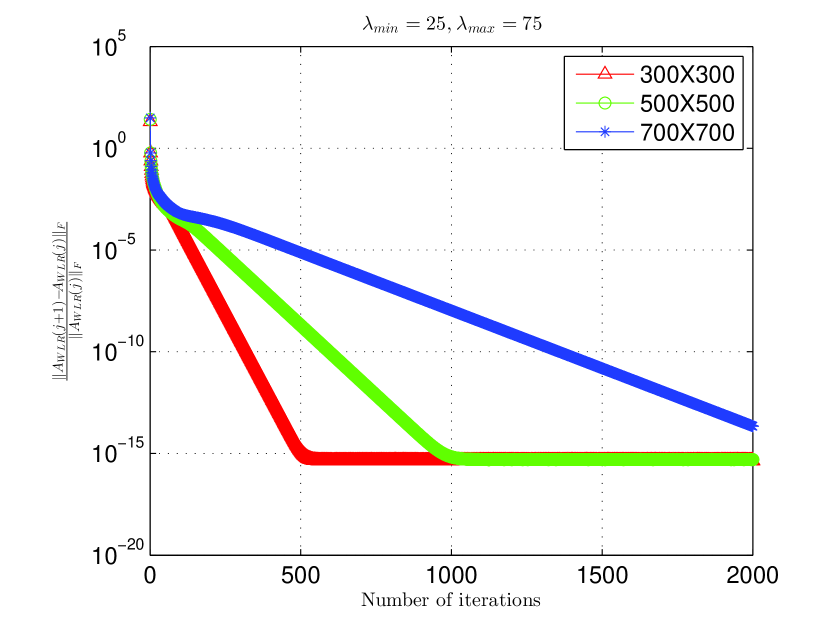
(a)

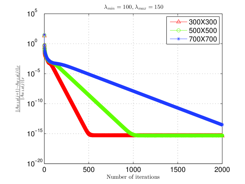
(b)

Fig. 1: Iterations vs Relative error: (a) $\lambda=25,\zeta=75$; (b) $\lambda=100,\zeta=150$.

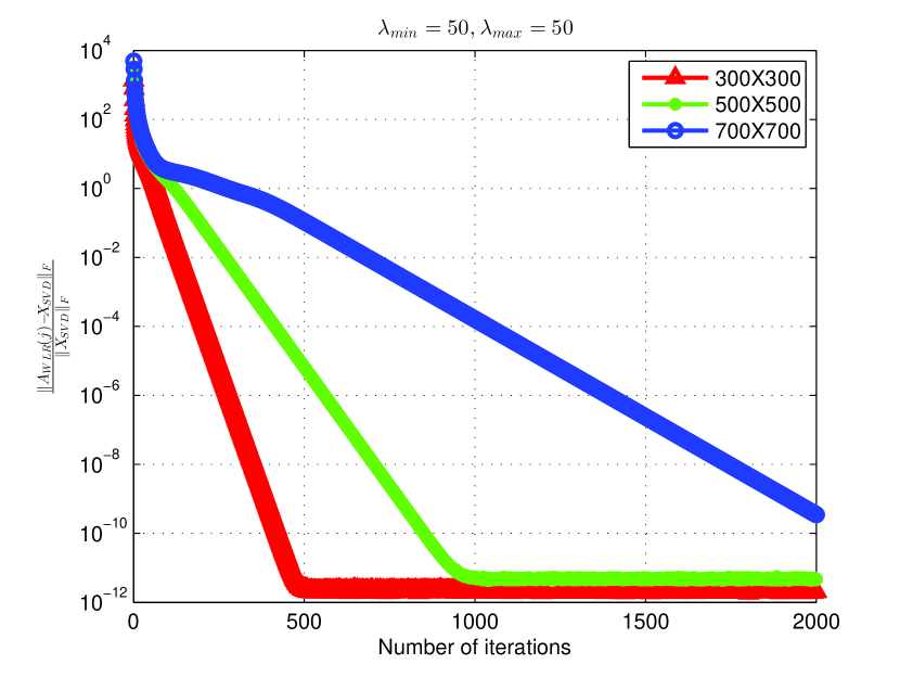
(a)

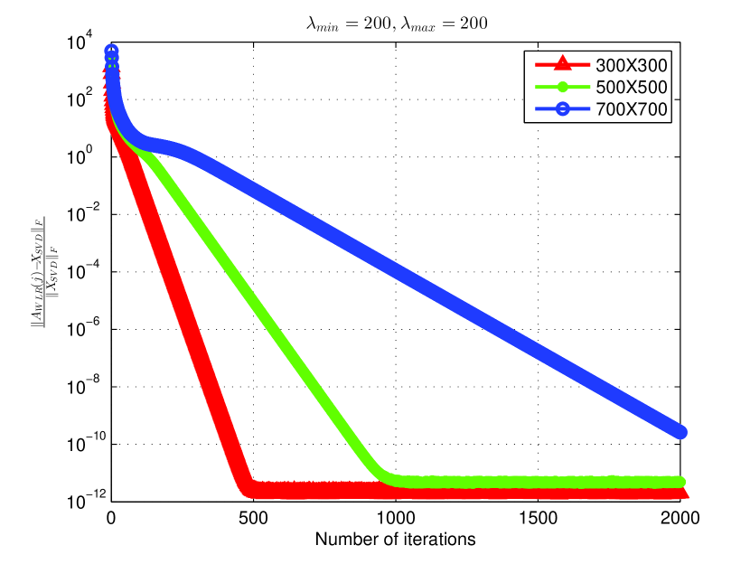
(b)

Fig. 2: Iterations vs $\frac{\|A_{WLR}(j)-X_{SVD}\|_{F}}{\|X_{SVD}\|_{F}}$: (a) $\lambda=50$; (b) $\lambda=200.$

Next, we consider a uniform weight in the first block $W_{1}$ and $W_{2}=\mathbbm{1}$. Recall that, in this case the solution to problem (7) can be given in closed form. That is, when $W_{1}=\lambda\mathbbm{1}$, the rank $r$ solutions to (7) are $X_{SVD}=[\frac{1}{\lambda}\tilde{X}_{1}\;\;\tilde{X}_{2}]$, where $[\tilde{X}_{1}\;\;\tilde{X}_{2}]$ is obtained in closed form using a SVD of $[\lambda A_{1}\;\;A_{2}]$. In Figure 5.2, we plot iterations versus $\frac{\|A_{WLR}(j)-X_{SVD}\|_{F}}{\|X_{SVD}\|_{F}}$ in logarithmic scale. From Figures 5.1 and 5.2 it is clear that the algorithm in Section 4.1 converges. Even for the bigger size matrices the iteration count is not very high to achieve the convergence.

5.4 Numerical results supporting Theorem 4

We now demonstrate numerically the rate of convergence as stated in Theorem 2.1 when the block of weights in $W_{1}$ goes to $\infty$ and $W_{2}=\mathbbm{1}$. First we use an uniform weight $W_{1}=\lambda\mathbbm{1}$ and $W_{2}=\mathbbm{1}$. The algorithm in Section 4 is used to compute $A_{WLR}$ and SVD is used for calculating $A_{G}$, the solution to (3) when $A=(A_{1}\;\;A_{2})$. We plot $\lambda$ vs. $\lambda\|A_{G}-A_{WLR}\|_{F}$ where $\lambda\|A_{G}-A_{WLR}\|_{F}$ is plotted in logarithmic scale along $Y$-axis. We run our algorithm 20 times with the same initialization and plot the average outcome. A threshold equal to $10^{-7}$ is set for the experiments in this subsection. For Figure 5.3 we set $\lambda=[1:50:1000]$.

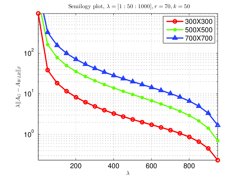
(a)

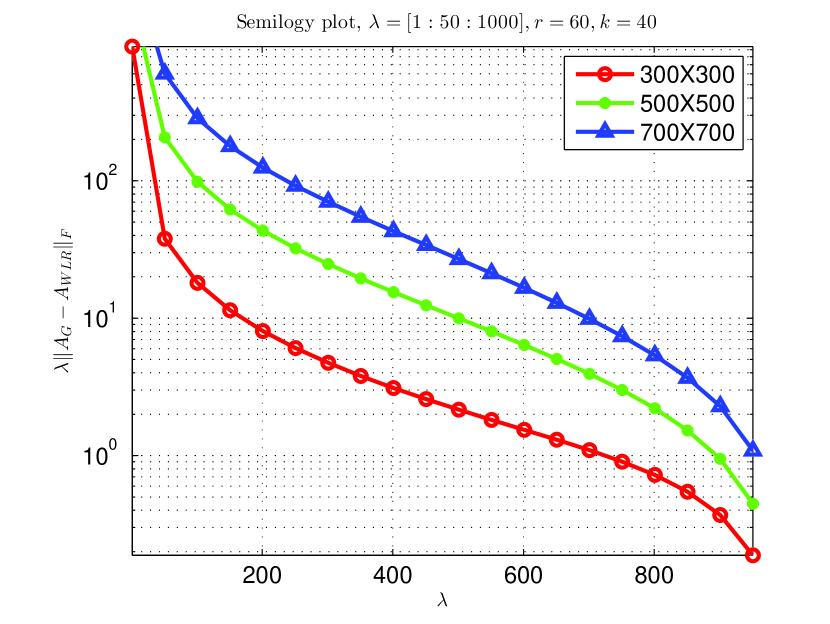
(b)

Fig. 3: $\lambda$ vs. $\lambda\|A_{G}-A_{WLR}\|_{F}$: (a) $(r,k)=(70,50)$, (b) $(r,k)=(60,40)$.

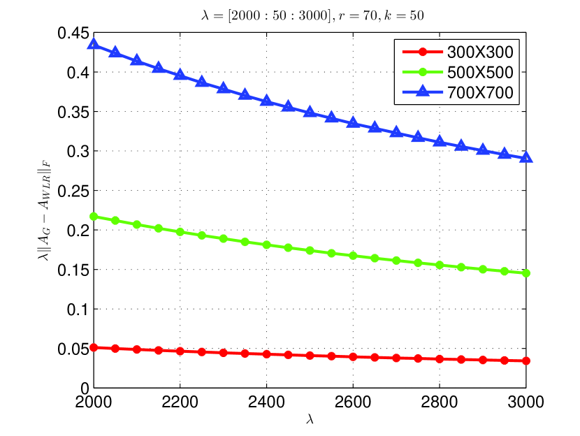
(a)

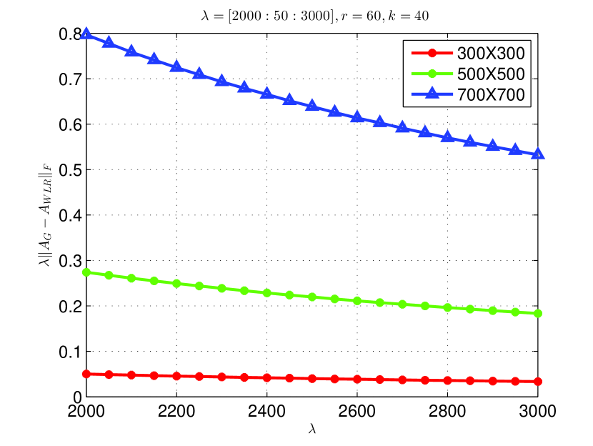
(b)

Fig. 4: $\lambda$ vs. $\lambda\|A_{G}-A_{WLR}\|_{F}$: (a) $(r,k)=(70,50)$, (b) $(r,k)=(60,40)$.

The plots indicate for an uniform $\lambda$ in $W_{1}$ the convergence rate is at least $O(\frac{1}{\lambda}),\lambda\to\infty.$ Next we consider a nonuniform weight in the first block $W_{1}$ and $W_{2}=\mathbbm{1}$. We consider $(W_{1})_{ij}\in[2000,2020],[2050,2070]$ and so on. For Figure 5.4, $\lambda\|A_{G}-A_{WLR}\|_{F}$ (recall $\min_{\begin{subarray}{c}1\leq i\leq m\\ 1\leq j\leq k\end{subarray}}(W_{1})_{ij}=\lambda$) is plotted in regular scale along $Y$-axis. The curves in figure 5.4 are not always strictly decreasing but it is encouraging to see that they stay bounded. Figures 5.3 and 5.4 provide numerical evidence in supporting Theorem 4. As established in Theorem 4 the above plots demonstrate the convergence rate is at least $O(\frac{1}{\lambda}),\lambda\to\infty.$

5.5 Comparison with state-of-the-art general weighted algorithms

In this section, we compare the performance of our special weighted algorithm on synthetic data with the standard weighted total alternating least squares (WTALS) method proposed in [21, 26] and the expectation maximization (EM) method proposed by Srebro and Jaakkola [9]. The existing algorithms are for general weighted case but for our purpose we consider partial weighting in them. Additionally, we compare the performance of our algorithm with the standard alternating least squares, WTALS, and the EM method [9, 21] for $k=0$ case. For the numerical experiments in this section, we are interested to see how the distribution of the singular values affects the performance of our algorithm compare to other state-of-the-art algorithms.

5.5.1 Performance compare to other weighted low-rank approximation algorithms

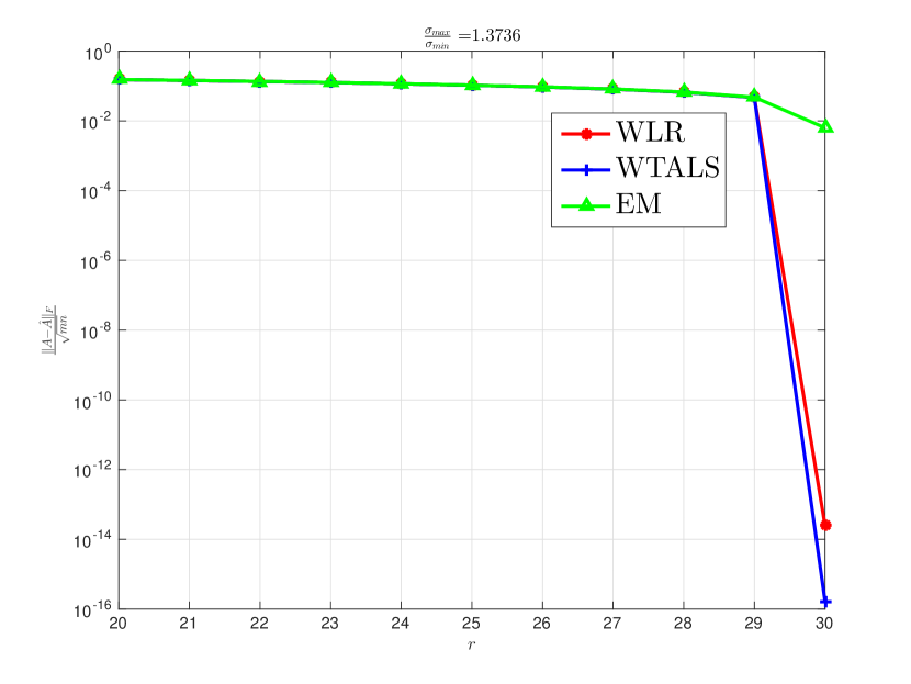
(a)

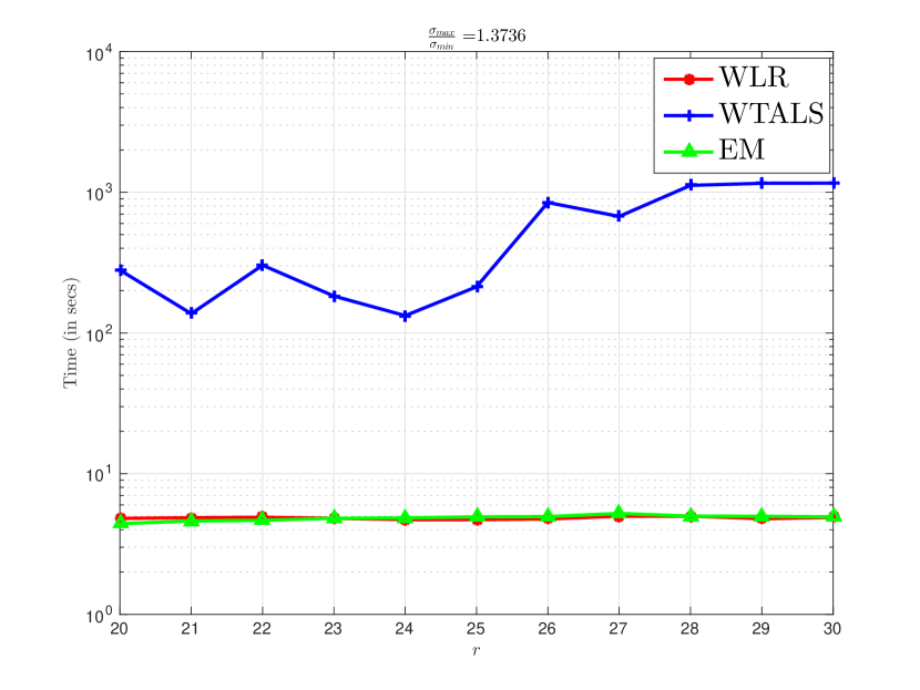
(b)

Fig. 5: Comparison of WLR with other methods when $\kappa(A)$ small: (a) $r$ versus RMSE, (b) $r$ versus time. We have $\kappa(A)=1.3736$, $r=[20:1:30]$, $k=10$, and $(W_{1})_{ij}\in[50,1000]$.

The weights in the first block are chosen randomly from a large interval. We set $(W_{1})_{ij}\in[50,1000]$ and $W_{2}=\mathbbm{1}$. For WTALS, as specified in the software package, we consider max_iter = 1000, threshold = 1e-10 [21]. For EM, we choose  max_iter = 5000, threshold = 1e-10, and for WLR, we set max_iter = 2500, threshold = 1e-16. For the performance measure, we use the standard root mean square error (RMSE) which is $\|A-\hat{A}\|_{F}/\sqrt{mn}$, where $\hat{A}\in\mathbb{R}^{m\times n}$ is the low-rank approximation of $A$ obtained by using different weighted low-rank approximation algorithm. The MATLAB code for the EM method is written by the authors following the algorithm proposed in [9]. For computational time of WLR and EM, the authors do not claim the optimized performance of their codes. However, the initialization of $X$ plays a crucial role in promoting convergence of the EM method to a global, or a local minimum, as well as the speed with which convergence is attained.

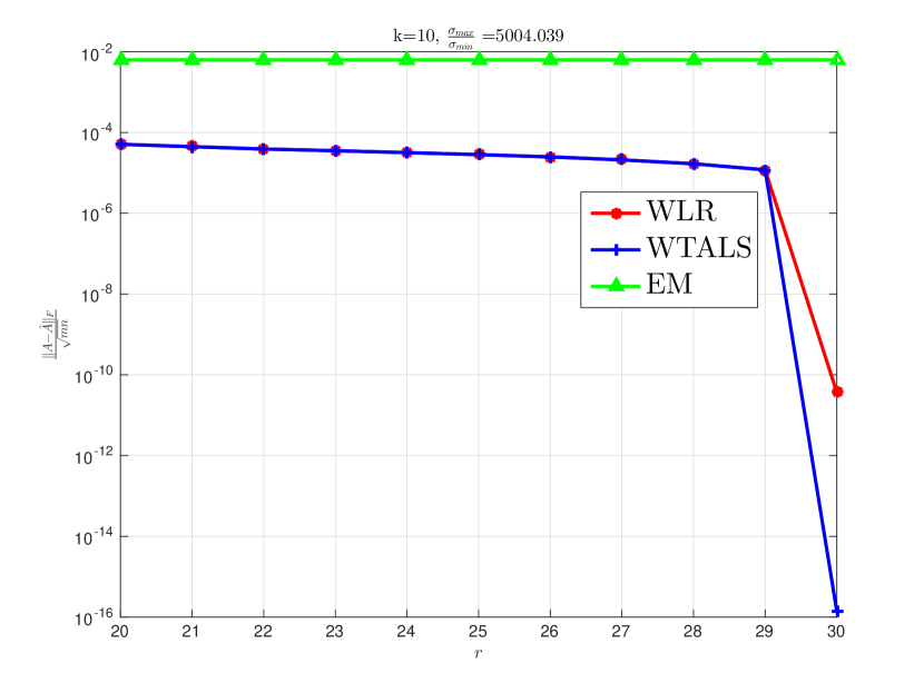
(a)

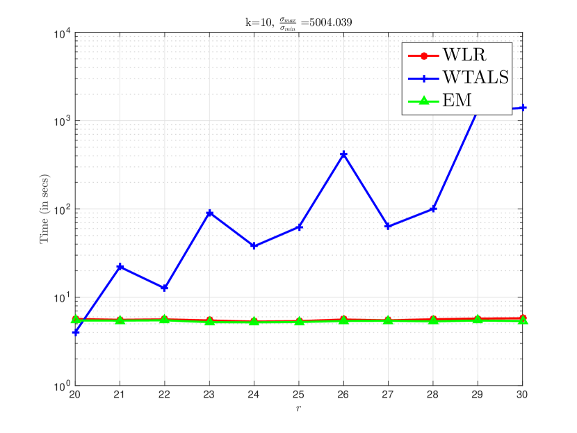
(b)

Fig. 6: Comparison of WLR with other methods when $\kappa(A)$ large: (a) $r$ versus RMSE, (b) $r$ versus time. We have $\kappa(A)=5.004\times 10^{3}$, $r=[20:1:30]$, $k=10$, and $(W_{1})_{ij}\in[50,1000]$.

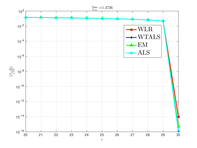
(a)

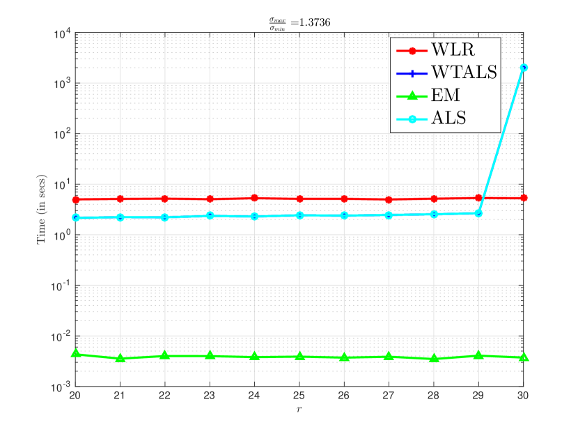
(b)

Fig. 7: Comparison of WLR with other methods for $k=0$ and $\kappa(A)$ small: (a) $r$ versus RMSE, (b) $r$ versus time. We have $\kappa(A)=1.3736$, $r=[20:1:30]$.

To implement the EM method, as mentioned in [9], first we rescale the weight matrix to $W_{EM}=\frac{1}{\max_{ij}(W_{1})_{ij}}(W_{1}\;\;\mathbbm{1})$. For a given threshold of weight bound $\epsilon_{EM}$, we initialize $X$ to a zero matrix if $\min_{ij}(W_{EM})_{ij}\leq\epsilon_{W_{EM}}$, otherwise we initialize $X$ to $A$. Initialization for WLR is same as specified in Section 5.2. To obtain the accurate result we run each experiment 10 times and plot the average outcome. Both RMSE and computational time are plotted in logarithmic scale along $Y$-axis. Figure 5.5 and 5.6 indicate that WLR is more efficient in handling bigger size matrices than WTALS [21] with the comparable performance measure. This can be attributed by the fact that WTALS uses a weight matrix of size $mn\times mn$ for the given input size $m\times n$, which is both memory and time inefficient. On the other hand, Figure 5.5 and 5.6 support the fact that as mentioned in [9], the EM method is computationally effective, however in some cases might converge to a local minimum instead of global.

5.5.2 Performance comparison for $k=0$ (Alternating Least Squares)

For $k=0$ we set the weight matrix as $W=\mathbbm{1}$ for all weighted low-rank approximation algorithm. Moreover, we include the classic alternating least squares algorithm to compare between the accuracy of the methods. As specified in Section 5.5.1, the stopping criterion for all weighted low-rank algorithms are kept the same and RMSE is used for performance measure. We run each experiment 10 times and plot the average outcome. Figure 5.7 and 5.8 indicate that WLR has comparable performance. However, the standard ALS, WTALS, and EM method is more efficient than WLR, as for $W=\mathbbm{1}$ case, each method uses SVD to compute the solution.

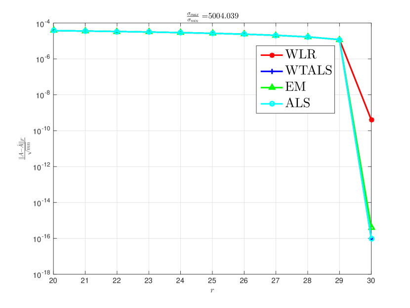
(a)

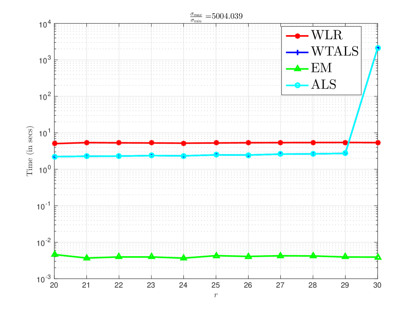
(b)

Fig. 8: Comparison of WLR with other methods for $k=0$ and $\kappa(A)$ large: (a) $r$ versus RMSE, (b) $r$ versus time. We have $\kappa(A)=5.004\times 10^{3}$, $r=[20:1:30]$.

5.5.3 Performance compare to constrained low-rank approximation of Golub-Hoffman-Stewart

As mentioned in our analytical results, one can expect, with appropriate conditions, the solutions to (7) will converge and the limit is $A_{G}$, the solution to the constrained low-rank approximation problem by Golub-Hoffman-Stewart. We now show the effectiveness of our special weighted algorithm compare to other state-of-the-art weighted low rank algorithms when $(W_{1})_{ij}\to\infty,$ and $W_{2}=\mathbbm{1}$. In this section, the weights in $W_{1}$ are chosen to be large to show effectiveness of our algorithm for large weighted case in the first block. SVD is used for calculating $A_{G}$, the solution to (3), when $A=(A_{1}\;\;A_{2})$, for varying $r$ and fixed $k$. Considering $A_{G}$ as the true solution we use the RMSE measure $\|A_{G}-\hat{A}\|_{F}/\sqrt{mn}$ as the performance metric, where $\hat{A}\in\mathbb{R}^{m\times n}$ is the low-rank approximation of $A$ obtained by different weighted low-rank algorithm. From Figure 5.9 it is evident that WLR has the superior performance compare to the other state-of-the-art general weighted low-rank approximation algorithms when $W_{1}\to\infty$.

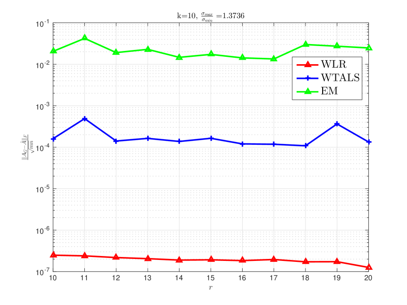
(a)

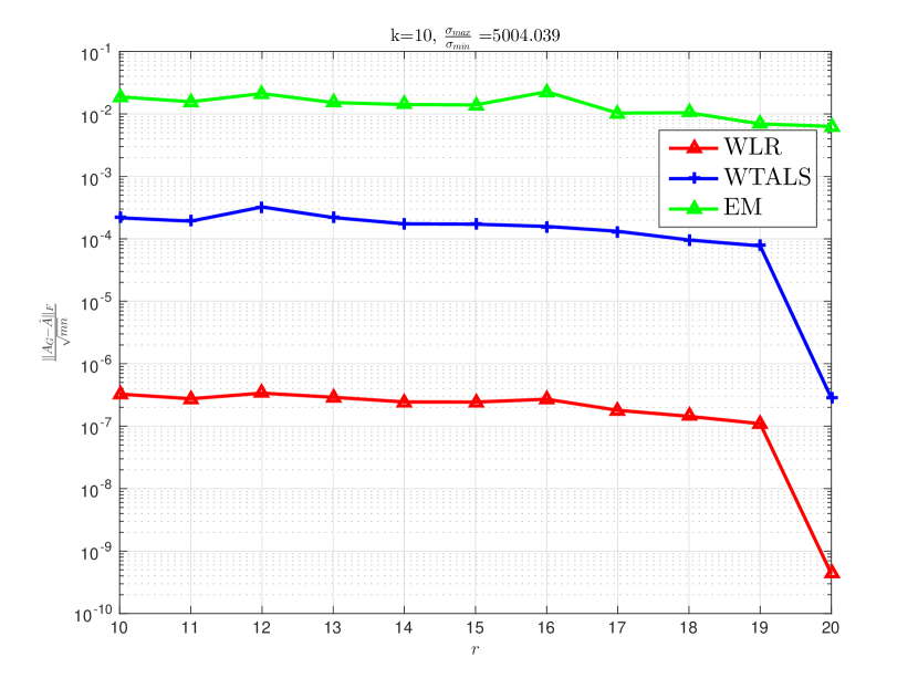
(b)

Fig. 9: $r$ vs $\|A_{G}-\hat{A}\|_{F}/\sqrt{mn}$ for different methods, $(W_{1})_{ij}\in[500,1000],W_{2}=\mathbbm{1}$, $r=10:1:20$, and $k=10$: (a) $\kappa(A)$ small, (b) $\kappa(A)$ large.

To conclude, WLR has comparable or superior performance compare to the existing general weighted low-rank approximation algorithms for the special case of weight with fairly less computational time. Even when the columns of the given matrix are not constrained, that is $k=0$, its performance is comparable to the standard ALS. Additionally, WLR and EM method can easily handle bigger size matrices and easier to implement for real world problems. On the other hand, WTALS requires more computational time and is not memory efficient to handle large scale data (see table 5.1). Another important feature of our algorithm is that it does not assume any particular condition about the matrix $A$ and performs equally well in every occasion.

Table 1: Average computation time (in seconds) for each algorithm to converge to $A_{G}$

$\kappa(A)$	WLR	EM	WTALS
1.3736	6.5351	6.1454	205.1575
$5.004\times 10^{3}$	8.8271	8.1073	107.0353

References

- [1] G. H. Golub, A. Hoffman, and G. W. Stewart, A generalization of the Eckart-Young-Mirsky matrix approximation theorem, Linear Algebra and its Applications, 88-89 (1987), pp. 317–327.
- [2] A. Dutta, X. Li, B. Gong, and M. Shah, Weighted singular value thresholding and its applications to background estimation, submitted.
- [3] A. Dutta and X. Li, Background estimation from video sequences using weighted low-rank approximation of matrices, submitted.
- [4] I. T. Jolliffee, Principal Component Analysis, Second edition, Springer-Verlag, 2002.
- [5] Z. Lin, M. Chen, and Y. Ma, The augmented Lagrange multiplier method for exact recovery of corrupted low-rank matrices, arXiv preprint arXiv1009.5055, 2010.
- [6] Per-ke Wedin, Perturbation bounds in connection with singular value decomposition, BIT Numerical Mathematics, 12-1(1972), pp. 99–111.
- [7] A. Dutta and X. Li, A Fast Algorithm for a Special Weighted Low Rank Approximation, submitted.
- [8] C. Eckart and G. Young, The approximation of one matrix by another of lower rank, Psychometrika, 1-3 (1936), pp. 211–218.
- [9] N. Srebro and T. Jaakkola, Weighted low-rank approximations, 20th International Conference on Machine Learning (2003), pp. 720–727.
- [10] G.W. Stewart, A second order perturbation expansion for small singular values, Linear Algebra and its Applications, 56 (1984), pp. 231–235.
- [11] A. Dutta, Weighted low-rank approximation of matrices: some analytical and numerical aspects, Ph.D. dissertation, Department of Mathematics, University of Central Florida, 2016.
- [12] C. Davis and W. Kahan, The rotation of eigenvectors by a perturbation III., SIAM Journal on Numerical Analysis, 7 (1970), pp. 1–46.
- [13] T. Okatani and K. Deguchi, On the Wiberg algorithm for matrix factorization in the presence of missing components, International Journal of Computer Vision, 72-3 (2007), pp. 329–337.
- [14] T. Wiberg, Computation of principal components when data are missing, In Proceedings of the Second Symposium of Computational Statistics (1976), pp. 229–336.
- [15] N. Srebro, J. D. M. Rennie, and T. S. Jaakola, Maximum-margin matrix factorization, In Proceedings of Advances in Neural Information Processing Systems, 18 (2005), pp. 1329–1336.
- [16] T. Hastie, R. Mazumder, J. Lee, and R. Zadeh, Matrix completion and low-rank SVD via fast alternating least squares, arXiv preprint arXiv1410.2596, 2014.
- [17] M. Udell, C. Horn, R. Zadeh, and S. Boyd, Generalized low-rank models, arXiv preprint arXiv:1410.0342, 2014.
- [18] J. Hansohm, Some properties of the normed alternating least squares (ALS) algorithm, Optimization, 19-5 (1988), pp. 683–691.
- [19] A. M. Buchanan and A. W. Fitzgibbon, Damped Newton algorithms for matrix factorization with missing data, In Proceedings of the 2005 IEEE Computer Society Conference on Computer Vision and Pattern Recognition, 2 (2005), pp. 316–322.
- [20] H. Liu, X. Li, and X. Zheng, Solving non-negative matrix factorization by alternating least squares with a modified strategy, Data Mining and Knowledge Discovery, 26-3 (2012), pp. 435–451.
- [21] I. Markovsky, J. C. Willems, B. De Moor, and S. Van Huffel, Exact and approximate modeling of linear systems: a behavioral approach, Number 11 in Monographs on Mathematical Modeling and Computation, SIAM, 2006.
- [22] I. Markovsky, Low-rank approximation: algorithms, implementation, applications, Communications and Control Engineering. Springer, 2012.
- [23] S. Van Huffel and J. Vandewalle, The total least squares problem: computational aspects and analysis, Frontiers in Applied Mathematics 9 , SIAM, Philadelphia, 1991.
- [24] K. Usevich and I. Markovsky, Variable projection methods for affinely structured low-rank approximation in weighted 2-norms, Journal of Computational and Applied Mathematics 272 (2014), pp. 430–448.
- [25] G.W. Stewart, On the asymptotic behavior of scaled singular value and QR decompositions, Mathematics of Computation, 43-168 (1984), pp. 483–489.
- [26] J. H. Manton, R. Mehony, and Y. Hua, The geometry of weighted low-rank approximations, IEEE Transactions on Signal Processing, 51-2 (2003), pp. 500–514.
- [27] W. S. Lu, S. C. Pei, and P. H. Wang, Weighted low-rank approximation of general complex matrices and its application in the design of 2-D digital filters, IEEE Transactions on Circuits and Systems I: Fundamental Theory and Applications, 44-7 (1997), pp.650–655.
- [28] D. Shpak, A weighted-least-squares matrix decomposition with application to the design of 2-D digital filters, In Proceedings of IEEE 33rd Midwest Symposium on Circuits and Systems, (1990), pp. 1070–1073.
- [29] K. Usevich and I. Markovsky, Optimization on a Grassmann manifold with application to system identification, Automatica, 50-6 (2014), pp. 1656–1662.
- [30] S. Brutzer, B. Höferlin, and G. Heidemann, Evaluation of background subtraction techniques for video surveillance, IEEE Computer Vision and Pattern Recognition (2011), pp. 1937–1944.
- [31] J. Wright, Y. Peng, Y. Ma, A. Ganseh, and S. Rao, Robust principal component analysis: exact recovery of corrupted low-rank matrices by convex optimization, Advances in Neural Information Processing systems 22, (2009), pp. 2080–2088.
- [32] G.W. Stewart and J. Sun, Matrix Perturbation Theory, Academic Press, Boston, 1990.