DPF2015-143 October 31, 2015

Forward $W+c,b$-jet and Top Measurements with LHCb

Philip Ilten

Massachusetts Institute of Technology
77 Massachusetts Avenue, Cambridge, MA 02139, USA

Inclusive $c$ and $b$-jet tagging algorithms have been developed to utilize the excellent secondary vertex reconstruction and resolution capabilities of the LHCb detector. The validation and performance of these tagging algorithms are reported using the full run 1 LHCb dataset at $7$ and $8\mathrm{\,Te\kern-1.00006ptV}$. Jet-tagging has been applied to $\mu+$jet final states to measure both the $W+c,b$-jet charge asymmetries and the ratios of $W+c,b$-jet to $W+$jet and $W^{\pm}+$jet to $Z+$jet production. The forward top production cross-section is also measured using the $\mu+b$-jet final. All results are found to be consistent with standard model predictions.

PRESENTED AT

DPF 2015
The Meeting of the American Physical Society
Division of Particles and Fields
Ann Arbor, Michigan, August 4–8, 2015

1 Introduction

Inclusive identification of jets originating from $c$ and $b$-quarks is a critical experimental technique needed for both standard model (SM) measurements such as the top cross-section, and beyond the standard model (BSM) searches, e.g. axigluon searches via charge asymmetries in di-$b$-jet production. LHCb is a forward arm spectrometer [1] located on the large hadron collider (LHC), with a pseudo-rapidity range of $2<\eta<5$ and initially designed to measure properties of $b$-hadron decays. Heavy-flavor jets typically contain secondary vertices from $c$ and $b$-hadron decays. With excellent secondary vertex reconstruction, LHCb is an ideal environment for $c,b$-jet tagging, while its forward coverage provides complementary results to the general purpose detectors on the LHC.

In these proceedings the LHCb $c,b$-jet tagging and its application to physics measurements in run 1 LHCb data is reported. Two main datasets recorded at different $pp$ collision energies are used here, a $1~{}\mbox{\,fb}^{-1}$ dataset at $\sqrt{s}=7\mathrm{\,Te\kern-1.00006ptV}$ recorded in $2011$ and a $2\mbox{\,fb}^{-1}$ dataset at $\sqrt{s}=8\mathrm{\,Te\kern-1.00006ptV}$ recorded in $2012$. In Section 2 the $c,b$-jet tagging algorithm, validation, and performance of [2] is outlined. Ratios of $W+c,b$-jet and $Z+$jet production using $\mu+$jet final states from [3] are presented in Section 3. Finally, a subsample of $\mu+b$-jet final state events with a tightened kinematic region is used to measure forward top-quark production cross-sections [4] in Section 4.

2 Heavy-Flavor Jet Tagging

In [2], heavy-flavor jets are tagged using $n$-body secondary vertices (SV) built from the tracks of charged particles. Two-body SVs are created from displaced tracks in the event with transverse momentum, $p_{\mathrm{T}}$, $>0.5\mathrm{\,Ge\kern-1.00006ptV}$, and must pass basic quality requirements. All SVs with shared tracks are combined to produce $n$-body SVs, such that tracks are unique to a single SV. Additional loose requirements, consistent with $c$ and $b$-hadron decays, are applied to these SVs. A jet is heavy-flavor tagged if the $\Delta R\equiv\sqrt{\Delta\phi^{2}+\Delta\eta^{2}}$ between the flight-direction for a SV and the jet momentum is less then the jet radius parameter, $R$. For these studies jets are built from particle flow input [5] with $R=0.5$ using the anti-$k_{\mathrm{T}}$ algorithm [6].

For each SV-tag the responses of two boosted decision trees (BDTs) are calculated; $\mbox{BDT}(bc|udsg)$ discriminates light-jets from $c,b$-jets and $\mbox{BDT}(b|c)$ separates $c$-jets from $b$-jets. Ten variables are used as input to the BDTs: SV mass, corrected mass, transverse flight distance, $p_{\mathrm{T}}(\mathrm{SV})/p_{\mathrm{T}}(\mathrm{j})$, $\Delta R$ between the jet momentum and $\mathrm{SV}$ flight-direction, number of tracks in the SV, number of SV tracks with $\Delta R<0.5$ to the jet, net charge of the SV, flight-distance $\chi^{2}$, and summed $\mathrm{IP}_{\chi^{2}}$ of the tracks in the SV. Example two-dimensional distributions from simulation of the $\mbox{BDT}(bc|udsg)$ and $\mbox{BDT}(b|c)$ responses for light, $c$, and $b$-jets are given in Figure 1. Light jets cluster at the origin, $c$-jets in the lower right, and $b$-jets in the upper right.

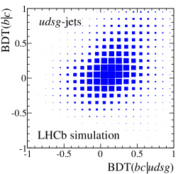
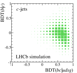
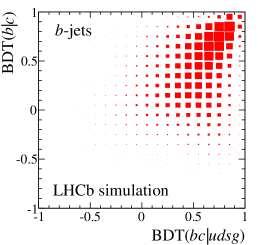
Figure 1: Two-dimensional distributions from LHCb simulation as a function of $\mbox{BDT}(bc|udsg)$ and $\mbox{BDT}(b|c)$ responses for (left) light, (middle) $c$, and (right) $b$-jets.

Four data samples are used for efficiency determination with the tag-and-probe method. Three are di-jet samples containing a tag-jet with a fully reconstructed $b$-hadron, a fully reconstructed $c$-hadron, or a displaced muon. The probe-jets of the $b$-hadron sample are $b$-enriched, while the probe-jets of the $c$-hadron and displaced muon samples are both $c$ and $b$-enriched. The fourth sample requires an isolated high-$p_{\mathrm{T}}$ tag-muon and a probe-jet, which is light-jet enhanced. The jet-tagging efficiency in each sample is the number of tagged probe-jets over the total number of probe-jets for a given jet type (light, $c$, or $b$).

The probe-jet flavor composition prior to SV-tagging is determined by fitting the $\log(\mathrm{IP}_{\chi^{2}})$ distributions for the hardest-$p_{\mathrm{T}}$ track or hardest $p_{\mathrm{T}}$-muon of the jet. After SV-tagging, the probe-jet flavor is determined by a two-dimensional fit of the $\mbox{BDT}(bc|udsg)$ and $\mbox{BDT}(b|c)$ response distribution. Projections of this fit onto the $\mbox{BDT}(b|c)$ and $\mbox{BDT}(bc|udsg)$ axes for the $c$-hadron sample are shown in Figure 2.

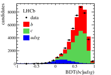
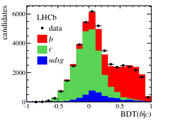
Figure 2: Projections of the two-dimensional BDT response fit onto the (left) $\mbox{BDT}(bc|udsg)$ and (right) $\mbox{BDT}(b|c)$ axes for the $c$-hadron sample. The stacked fills are (blue) light, (green) $c$, and (red) $b$-jet templates from simulation.

There is good agreement between the tagging efficiencies obtained from data and simulation. After SV-tagging a jet, either the BDT distribution can be fit directly, or further requirements can be placed on the $\mbox{BDT}(bc|udsg)$ and $\mbox{BDT}(b|c)$ responses when high-purity samples are needed. On the left of Figure 3 the efficiency from data for tagging a $c$ and $b$-jet with an SV is plotted as a function of jet $p_{\mathrm{T}}$. By varying the minimum requirement of $\mbox{BDT}(bc|udsg)$, the tagging efficiency from simulation as a function of the light-jet mis-tag rate is given on the right of Figure 3.

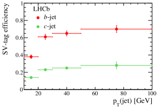
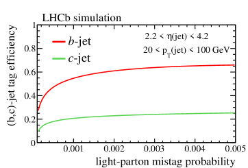
Figure 3: Tagging efficiency for $c,b$-jets (right) from data as a function of jet $p_{\mathrm{T}}$, and (left) from simulation as a function of light-jet mis-tag rate.

The primary uncertainty on the tagging efficiency is from the $\log(\mathrm{IP}_{\chi^{2}})$ fits prior to SV-tagging, and is evaluated by fixing the light-jet component from the high-$p_{\mathrm{T}}$ muon sample. Systematic uncertainties from BDT templates, $\mathrm{IP}$ resolution, muon mis-identification, gluon splitting, and number of $pp$ interactions have also been evaluated. For jets with $p_{\mathrm{T}}>20\mathrm{\,Ge\kern-1.00006ptV}$, the total systematic uncertainty on the tagging efficiency is found to be $\approx 10\%$ for both $c$ and $b$-jets.

3 $\bm{W+c,b}$-jet Ratios

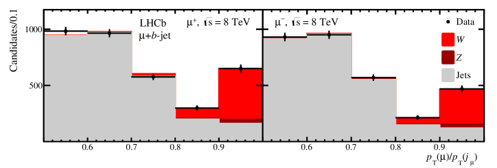
Figure 4: Isolation distributions and their corresponding template fits for the (left) $\mu^{+}+b$-jet and (right) $\mu^{-}+b$-jet at $\sqrt{s}=8\mathrm{\,Te\kern-1.00006ptV}$. The stacked fills are the (gray) di-jet, (light red) $W+b$-jet, and (dark red) $Z+b$-jet templates.

Measuring $W+c,b$-jet production not only constrains the $s$-quark PDF of the proton, but also helps determine backgrounds to top production and understand high-$p_{\mathrm{T}}$ $b$-jet production. In [3] the fiducial definition of a $W+$jet event requires a muon with $p_{\mathrm{T}}(\mu)>20\mathrm{\,Ge\kern-1.00006ptV}$ and $2<\eta(\mu)<4.5$, and a jet with $p_{\mathrm{T}}(j)>20\mathrm{\,Ge\kern-1.00006ptV}$ and $2.2<\eta(j)<4.2$. The reduced $\eta$ range of the jet ensures stable reconstruction and tagging efficiencies. Additionally, the $\Delta R$ between the muon and jet must be greater than $0.5$ and the combined $p_{\mathrm{T}}$ of the muon and jet, $p_{\mathrm{T}}(\mu+j)$, must be greater than $20\mathrm{\,Ge\kern-1.00006ptV}$. Here $p_{\mathrm{T}}(\mu+j)>20\mathrm{\,Ge\kern-1.00006ptV}$ is a theoretically well-defined proxy for the experimental-level selection $p_{\mathrm{T}}(j_{\mu}+j)>20\mathrm{\,Ge\kern-1.00006ptV}$, where $j_{\mu}$ is the jet containing the muon. The $p_{\mathrm{T}}(j_{\mu}+j)$ requirement reduces $p_{\mathrm{T}}$-balanced di-jet backgrounds, where energy is not lost to a missing neutrino.

Events are selected by requiring the hardest-$p_{\mathrm{T}}$ muon candidate, and the hardest-$p_{\mathrm{T}}$ non-muon candidate jet from the same primary vertex, satisfy all fiducial requirements with the substitution $p_{\mathrm{T}}(j_{\mu}+j)$ for $p_{\mathrm{T}}(\mu+j)$. Events are binned as a function of isolation, $p_{\mathrm{T}}(\mu)/p_{\mathrm{T}}(j_{\mu})$. The $\mu+c,b$ content of each bin is determined by requiring only events with an SV-tagged jet and performing the BDT fit of Figure 2. The isolation distribution of the full sample is fit to determine the $W+$jet yield, while the $\mu+c,b$-jet distributions are fit to determine the $W+c,b$-jet yields. The fits are split by muon charge and performed separately for the $7\mathrm{\,Te\kern-1.00006ptV}$ and $8\mathrm{\,Te\kern-1.00006ptV}$ datasets. In Figure 4 the $\mu+c,b$-jet isolation distribution fits at $\sqrt{s}=8\mathrm{\,Te\kern-1.00006ptV}$ are provided, where good agreement can be seen between the data and fit.

The measured $W+c,b$-jet asymmetries, $W+c,b$-jet to $W+$jet ratios, and $W+$jet to $Z+$jet ratios are,

where the first uncertainty is statistical and the second is systematic. The asymmetry $\mathcal{A}(Wq)$ is defined as $(\sigma(W^{+}q)-\sigma(W^{-}q))/(\sigma(W^{+}q)+\sigma(W^{-}q))$.

All measurements are unitless. Each observable is graphically compared to its SM prediction using the difference between experiment and theory over the maximum theory uncertainty; the points are this quantity, the gray and black bars are the total and statistical experimental uncertainties, and the asymmetric colored bands are the theory uncertainties. The SM predictions are calculated with the four-flavor scheme at NLO using MCFM [7] and the CT10 PDF set [8], where the total uncertainty is the combined PDF, $\alpha_{s}$, and scale uncertainty.

Because these measurements are ratios, most reconstruction efficiencies cancel. However, the $c,b$-tagging efficiencies, taken from Section 2, enter the $\sigma(Wc,b)/\sigma(Wj)$ ratios. For the $\sigma(Wc)/\sigma(Wj)$ ratio, the $c$-tagging efficiency is the primary systematic uncertainty, while the subtraction of top backgrounds from a sideband is the primary uncertainty for the $\sigma(Wb)/\sigma(Wj)$ measurement. Backgrounds from $\tau$ decays are subtracted from the $W+c$-jet measurements but are negligible. The primary uncertainty on both the asymmetries and the $Wj/Zj$ ratios is from the isolation fits.

4 Top Cross-Section

A tightened fiducial region of $p_{\mathrm{T}}(\mu)>25\mathrm{\,Ge\kern-1.00006ptV}$ and $50<p_{\mathrm{T}}(j)<100$ is applied to the analysis of Section 3 in [4] to obtain a top-quark enriched data sample; the top quarks are from both single top ($\approx 25\%$) and top-pair production ($\approx 75\%$). The additional muon requirement reduces the di-jet background, while the jet requirement suppresses direct $W+b$-jet background. The jet is required to be SV-tagged and the $\mu+b$-jet yield is determined from the isolation distribution via the methods of Section 3.

Despite the increased jet $p_{\mathrm{T}}$ requirement, a sizable background from direct $W+b$-jet production, i.e. not from top, remains in the $W+b$-jet yield. This background is constrained by determining the $W+$jet yield from data without an SV-tag, applying the $b$-tag efficiency, and correcting with the ratio $\sigma(Wb)/\sigma(Wj)$ from theory. Here, the theoretical uncertainty on $\sigma(Wb)/\sigma(Wj)$ is considerably smaller than for $\sigma(Wb)$ alone. This method is cross-checked against the $W+c$-jet yield, where no top production is present, and is found to describe the data well.

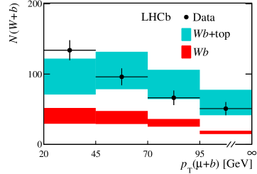
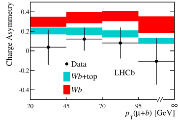
Figure 5: Combined $7$ and $8\mathrm{\,Te\kern-1.00006ptV}$ distributions of (left) the number of events as a function of $p_{\mathrm{T}}(\mu+b)$ and (right) the asymmetry, also as a function of $p_{\mathrm{T}}(\mu+b)$. The points are data, while the fills are the SM predictions for (red) $W+b$-jet production without top and (cyan) $W+b$-jet production with top.

In the left plot of Figure 5 the $W+b$-jet yield from the combined $7$ and $8\mathrm{\,Te\kern-1.00006ptV}$ data is plotted as a function of the muon and $b$-jet $p_{\mathrm{T}}$. The red band, with uncertainty, is the constrained $W+b$-jet prediction without top, while the cyan band, also with uncertainty, includes the SM top prediction. The yield, particularly at high $p_{\mathrm{T}}(\mu+b)$ cannot be described by direct $W+b$-jet production alone. Similarly, the asymmetry as a function of $p_{\mathrm{T}}(\mu+b)$ is plotted on the left of Figure 5. Here, the direct $W+b$-jet asymmetry is near $\approx 1/3$ due to valence quark content, while the top-pair asymmetry is $\approx 0$. Again, the direct $W+b$-jet hypothesis without top production does not describe the data well.

A binned profile likelihood fit of these two distributions is performed with the top contribution allowed to vary freely. Systematic uncertainties, both theoretical and experimental, are introduced as Gaussian nuisance parameters, and the SM hypothesis with and without top is compared. A $5.4\sigma$ significance is observed, indicating the presence of top production in the forward region. The top yield is then determined by subtracting the direct $W+b$-jet contribution constrained from data.

Correcting for reconstruction efficiencies, the $7$ and $8\mathrm{\,Te\kern-1.00006ptV}$ measured top cross-sections are,

where the first uncertainty is statistical and the second is the combined experimental and theoretical systematic uncertainties. Just as for the $W+c,b$-observables, each top cross-section is also graphically compared to its corresponding SM prediction calculated at NLO using MCFM with the four-flavor scheme. The primary systematic uncertainty is from the $b$-tagging efficiency, but the systematic uncertainties between the $7$ and $8\mathrm{\,Te\kern-1.00006ptV}$ measurements are nearly completely correlated.

5 Conclusion

Inclusive $c$ and $b$-jet tagging has been developed and validated using run 1 data from LHCb. This tagging in turn has been used to measure $W+c,b$-jet ratios and asymmetries as well as forward top production cross-sections. With significantly increased statistics during run 2 of the LHC, updates of these measurements will have significant physics impact, including constraining both $s$-quark and gluon PDFs, probing intrinsic $b$-content, and even possibly measuring the non-zero top-pair asymmetry. Further studies are underway to further improve tagging efficiencies as well as determine physics measurements that can utilize inclusive $c$-tagging.

References

- [1] LHCb collaboration, A. A. Alves Jr. et al., The LHCb detector at the LHC, JINST 3 (2008) S08005
- [2] LHCb collaboration, R. Aaij et al., Identification of beauty and charm quark jets at LHCb, JINST 10 (2015) P06013, arXiv:1504.07670
- [3] LHCb collaboration, R. Aaij et al., Study of boson production in association with beauty and charm, Phys. Rev. D92 (2015) 052012, arXiv:1505.04051
- [4] LHCb collaboration, R. Aaij et al., First observation of top quark production in the forward region, Phys. Rev. Lett. 115 (2015) 112001, arXiv:1506.00903
- [5] LHCb collaboration, R. Aaij et al., Study of forward +jet production in collisions at TeV, JHEP 01 (2014) 033, arXiv:1310.8197
- [6] M. Cacciari, G. P. Salam, and G. Soyez, The Anti-k(t) jet clustering algorithm, JHEP 04 (2008) 063, arXiv:0802.1189
- [7] J. M. Campbell and R. K. Ellis, Radiative corrections to Z production, Phys. Rev. D62 (2000) 114012, arXiv:hep-ph/0006304
- [8] H.-L. Lai et al., New parton distributions for collider physics, Phys. Rev. D82 (2010) 074024, arXiv:1007.2241