Entanglement properties of correlated random spin chains and similarities with conformally invariant systems

Abstract

We study the Rényi entanglement entropy and the Shannon mutual information for a class of spin-1/2 quantum critical XXZ chains with random coupling constants which are partially correlated. In the XX case, distinctly from the usual uncorrelated random case where the system is governed by an infinite-disorder fixed point, the correlated-disorder chain is governed by finite-disorder fixed points. Surprisingly, we verify that, although the system is not conformally invariant, the leading behavior of the Rényi entanglement entropies are similar to those of the clean (no randomness) conformally invariant system. In addition, we compute the Shannon mutual information among subsystems of our correlated-disorder quantum chain and verify the same leading behavior as the $n=2$ Rényi entanglement entropy. This result extends a recent conjecture concerning the same universal behavior of these quantities for conformally invariant quantum chains. For the generic spin-1/2 quantum critical XXZ case, the true asymptotic regime is identical to that in the uncorrelated disorder case. However, these finite-disorder fixed points govern the low-energy physics up to a very long crossover length scale and the same results as in the XX case apply. Our results are based on exact numerical calculations and on a numerical strong-disorder renormalization group.

I Introduction

The entanglement entropy has been proven as an important tool to study and classify statistical mechanics and condensed matter systems. For pure state systems, the most used measure of the entanglement between two complementary regions ${\cal A}$ and ${\cal B}$ is the so-called Rényi entanglement entropy

$$S_{n}\left({\cal A},{\cal B}\right)=\frac{1}{1-n}\ln{\rm Tr}\rho_{{\cal A}}^{n},$$ (1)

with $\rho_{{\cal A}}={\rm Tr}_{{\cal B}}\rho$ being the reduced density matrix of subsystem ${\cal A}$. For $n\rightarrow 1$, it recovers the von Neumann entanglement entropy $S_{1}=S_{{\rm vN}}=-{\rm Tr}\rho_{{\cal A}}\ln\rho_{{\cal A}}$.

In the arena of one-dimensional conformally invariant quantum systems, such measure allows us to identify the various distinct universality classes of critical behavior Holzhey et al. (1994); Calabrese and Cardy (2004). It is now understood that the ground state entanglement entropy reads Calabrese et al. (2010); Xavier and Alcaraz (2011)

$$S_{n}\left(x,L\right)=\frac{c}{6}\left(1+\frac{1}{n}\right)\ln f_{L}^{{\rm CFT}}(x)+\kappa_{1}+\frac{\left(-1\right)^{x}\kappa_{2}}{\left(f_{L}(x)\right)^{\phi/n}}+\dots,$$ (2)

where $c$ is the universal central charge of the underlying conformal field theory (CFT), $L$ is the system size (here, we consider periodic boundary conditions), $1\ll x\leq L/2$ is the size of the subsystem ${\cal A}$ , $f_{L}^{{\rm CFT}}\left(x\right)=\frac{L}{\pi}\sin\left(\frac{\pi x}{L}\right)$ is the scaling function (which equals the chord length), $\kappa_{1,2}$ are nonuniversal constants, and $\phi$ is related to the scaling dimension of the energy operator. For $n=1$ or for systems without a Fermi surface, $\kappa_{2}=0$.

However, there is no simple way of accessing the Rényi entanglement entropy directly from experimental measurements. It is then desirable to study other information measures that can be, in principle, directly observed in experiments, and, like $S_{n}$, enable us to determine the critical universality class of the system. Recently, the Shannon mutual information was proposed as one such information measure Alcaraz and Rajabpour (2013, 2014). It is defined as

$$I\left({\cal A},{\cal B}\right)={\rm Sh}\left({\cal A}\right)+{\rm Sh}\left({\cal B}\right)-{\rm Sh}\left({\cal A}\cup{\cal B}\right),$$ (3)

where ${\rm Sh}\left({\cal A}\right)=-\sum_{m}p_{m}\ln p_{m}$ is the usual Shannon entropy, with $p_{m}$ being the probability of finding the subsystem ${\cal A}$ in a configuration $m$ obtained from the normalized wave function $\left|\psi_{{\cal A}\cup{\cal B}}\right\rangle=\sum_{m,n}c_{m,n}\left|\phi_{{\cal A}}\right\rangle_{m}\otimes\left|\phi_{{\cal B}}\right\rangle_{n}$, namely $p_{m}=\sum_{n}\left|c_{m,n}\right|^{2}$. In general the Shannon entropy is a basis-dependent quantity. However, it was conjectured that $I({\cal A},{\cal B})$, in some special bases, shares the same leading asymptotic behavior as $S_{2}$ given by Eq. (2). This result was verified numerically for several quantum chains in distinct universality classes. 

The entanglement properties of quantum critical random (quenched disordered) systems are much less understood. All our knowledge is related to random spin chains governed by exotic infinite-randomness fixed point (IRFP) Fisher (1994, 1995). Since the ground state of these fixed points can be understood as a collection of nearly independent spin clusters arranged in a fractal fashion, it can be easily shown that $S_{n}\sim\gamma\ln f_{L}^{{\rm IRFP}}\left(x\right)$, with $\gamma=\ln 2$ being a universal $n$-independent constant Refael and Moore (2004); Laflorencie (2005); Hoyos and Rigolin (2006); Santachiara (2006); Hoyos et al. (2007); Bonesteel and Yang (2007); Fidkowski et al. (2008); Fagotti et al. (2011); Tran and Bonesteel (2011); Pouranvari and Yang (2013); Ramírez et al. (2014) in contrast to the clean system [see Eq. (2)]. This understanding stems exclusively from the analytical tool of the strong-disorder renormalization-group (SDRG) method Ma et al. (1979); Dasgupta and Ma (1980); Bhatt and Lee (1982) which can be used to compute $S_{n}$ Refael and Moore (2004); Hoyos et al. (2007). More recently, the scaling function $f_{L}^{{\rm IRFP}}(x)$ have been studied and shown to differ from the chord length Fagotti et al. (2011), namely

$$f_{L}^{{\rm IRFP}}\left(x\right)\approx\frac{L}{\pi}\left(\sin\left(\frac{\pi x}{L}\right)-0.153\sin^{3}\left(\frac{\pi x}{L}\right)\right).$$ (4)

The entanglement properties of quantum critical random systems governed by conventional finite-disorder fixed points are much less known. A possible reason is due to the lack of simple analytical and numerical tools for handling them. Examples of such systems are frustrated spin ladders or quantum spin chains with random ferro- and antiferromagnetic interactions which are of great interest from the experimental Nguyen et al. (1996); Irons et al. (2000); Koteswararao et al. (2010) and theoretical Westerberg et al. (1997); Yusuf and Yang (2003); Hoyos and Miranda (2004); Lavarélo et al. (2013) points of view. However, even though a strong-disorder renormalization-group description of these systems is possible, unlike the infinite-disorder case, the entanglement entropy $S_{n}$ cannot be computed in a simple way.

Apparently, the only known system governed by a finite-disorder fixed point whose entanglement properties were studied, namely the von Neumann entropy $S_{1}$, is the quantum Ising chain with correlated disorder Binosi et al. (2007). In this special case it is understood that disorder correlation prevents the generation of random mass, yielding thus a perturbatively irrelevant disorder Hoyos et al. (2011). Further increase of the disorder strength, beyond the perturbative limit, drives the system towards a line of finite-disorder critical fixed points. Interestingly, along this line, the ground state entanglement entropy increases.

In this paper we report an extensive study of Rényi entanglement entropy $S_{n}(x,L)$ and of the Shannon mutual information $I(x,L)$ for the critical XX spin chain (which is equivalent to a doubled quantum Ising chain at criticality) with correlated disorder. We show that $S_{n}$ exhibts the same leading finite-size scaling function $f_{L}^{{\rm CFT}}$ as in (2) with a different prefactor (effective central charge), in contrast to the infinite-randomness case (4). In addition, our results indicate that the Shannon mutual information $I(x,L)$ shares the same asymptotic behavior as $S_{2}$, as conjectured for the conformally invariant clean system. Furthermore, we show that these features are not exclusive particularities of the noninteracting XX model but are also present in the critical phase of the XXZ spin-1/2 chain below a relatively large crossover length.

The remainder of this article is organized as follows. In Sec. II we introduce the model and the numerical methods used. In Sec. III we compute the dynamical critical exponent, that indicates the presence of a line of finite-disorder fixed points. The entanglement measures $S_{n}$ and $I$ are computed in Sec. IV, and their dependence on the disorder strength and anisotropy is analyzed in detail. Our SDRG study is reported in Sec. V, where we derive the renormalization-group procedure and explain its numerical implementation for very large chains. Conclusions and final remarks are given in Sec. VI. For completeness, in Appendices A and B we compute the entanglement measures for random singlet states, and our SDRG decimation rules, respectively.

II The model and methods

We are interested in the ground state entanglement properties of the XXZ spin-1/2 chain given by the Hamiltonian

$$H=\sum_{i=1}^{L}J_{i}\left(S_{i}^{x}S_{i+1}^{x}+S_{i}^{z}S_{i+1}^{z}+\Delta S_{i}^{z}S_{i+1}^{z}\right),$$ (5)

where $\mathbf{S}_{i}$ are spin-1/2 operators. The lattice size is $L$ (even) and we consider periodic boundary conditions $\mathbf{S}_{L+1}=\mathbf{S}_{1}$. The anisotropy $\Delta$ is site independent and we constrain our analysis to $-1<\Delta\leq 1$, a region where the clean model is critical and conformally invariant. Quenched disorder is implemented via the coupling constants $J_{i}$ which are drawn from the distributions

$$P(J)=\frac{1}{D\Omega_{I}}\left(\frac{\Omega_{I}}{J}\right)^{1-1/D},\mbox{ with }0<J<\Omega_{I}.$$ (6)

Here, the disorder strength is parametrized by $D$ and $\Omega_{I}$ sets the energy scale. Correlation among the disorder variables is implemented as follows. All odd-numbered coupling constants are independent random variables drawn from Eq. (6). The even-numbered couplings, however, are equal to the odd one to their left, i.e., $J_{2i}=J_{2i-1}$. In this way, the sequence of couplings in our random correlated spin chain reads $J_{1},J_{1},J_{3},J_{3},\dots J_{L-1},J_{L-1}$.

As shown in Ref. Hoyos et al., 2011, for weak disorder $D\leq D_{c}\approx 0.3$ and for the XX model ($\Delta=0$), the system is governed by the clean critical point. For larger disorder values $D>D_{c}$, a line of finite-disorder fixed points is accessed. This contrasts with the uncorrelated case ($J_{i}$ are independent random variables $\forall i$), where disorder is perturbatively relevant and drives the system to a random singlet state described by a universal renormalization-group fixed point of infinite-randomness nature Fisher (1994).

The essence of this difference is the absence of a random mass in the former case. For $\Delta=0$, the energy mass gap is given by a function of the ratio between the products of even- and odd-numbered couplings Pfeuty (1979): $m\sim\sum_{i=1}^{L/2}\ln(J_{{\rm 2i}}/J_{{\rm 2i+1}})$. Therefore, it is reasonable to define $m_{x}=\overline{\ln J_{{\rm odd}}}-\overline{\ln J_{{\rm even}}}$ (where $\overline{\cdots}$ means the average over a coarse-grained region $x$) as a measure of the local distance from criticality, i.e., the local mass. This is the argument used in Ref. Hoyos et al., 2011 to ensure that the effective action of the system does not contain a random mass term. In the generic case $\Delta\neq 0$, the dependence of mass gap $m$ on the random couplings $J_{i}$ is not known. Presumably, it depends on the anisotropy $\Delta$ and will not be given just by a simple ratio among products of $J_{i}$. We then expect that the disorder couples to the mass term, and therefore the true ground state should be a random singlet just like in the uncorrelated disorder case. As we will see below, however, the random mass term seems to be quite small, and its effects are only seen at very low energy scales (very large chains). Hence, the physics of the quenched disordered quantum XXZ spin-1/2 chain without random mass can be studied in the preasymptotic regime of smaller chains.

The model in Eq. (5) is studied via two complementary methods: exact diagonalization (see Secs. III and IV) and strong-disorder renormalization group (see Sec. V).

In the case $\Delta=0$, a map to free fermions enables us to exactly diagonalize the system for quite large sizes. For $\Delta\neq 0$, we use the power method to evaluate the low-lying states up to system sizes $L=22$. Since the fixed points are of finite-disorder nature, the statistical fluctuations are much weaker as compared to those of the infinite-disorder fixed point. Then, disorder averaging over $N=10^{3}$ samples is sufficient for a reasonable accuracy in most of the cases.

When we use the SDRG method, the anisotropy values $\Delta=0$ and $\Delta\neq 0$ can be treated on an equal footing and chains of sizes $L=10^{6}$ and $10^{7}$ can be easily reached.

III The dynamical critical exponent

In this section we compute the dynamical critical exponent $z$ obtained from the leading behavior of the finite-size energy gap

$$\Delta E\sim L^{-z},$$ (7)

which is plotted in Fig. 1 for the anisotropy $\Delta=1/2$ and the disorder strengths $D=0.5$ and $2$. The continuous lines in the figure are the best fits for $z$.

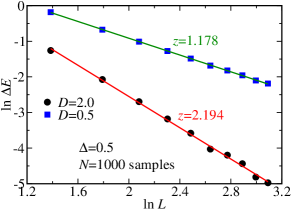
Figure 1: (Color online) Finite-size gap $\Delta E$ for various system sizes $L=4,6,8,\dots,22$, for the cases of disorder strength $D=0.5$ (blue squares) and $2.0$ (black circles) and anisotropy $\Delta=0.5$. The lines are the best linear fits, and the corresponding estimated values of $z$ are also shown.

It is important to remark that there is no crossover length $\xi$, in contrast with the uncorrelated disorder case. In the latter case, the true infinite-randomness fixed point is reached only when $L$ exceeds a disorder-dependent crossover length $\xi$. Below this length, the clean fixed point governs the system. Differently from Fig. 1, we would get a dynamical critical exponent $z=1$ for $L\ll\xi$ that crosses over to $z\rightarrow\infty$ for $L\gg\xi$. This crossover phenomena is observed in many quantities for the case of uncorrelated disorder Laflorencie et al. (2004); Hoyos et al. (2007). However, in the case of correlated disorder, such crossover behavior is absent.

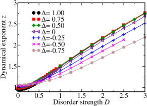
Figure 2: (Color online) Dynamical exponent $z$ as a function of the disorder strength $D$ for several anisotropy parameter $\Delta$. The results were obtained from the fit of the finite-size gap as in Fig. 1. The estimated error bars are of the order of the symbol sizes and the lines are guides to the eyes.

The critical exponent $z$ is plotted in Fig. 2 for various disorder strengths $D$ and anisotropies $\Delta$. As can be noticed, for $D<D_{c}\left(\Delta\right)$ the exponent $z$ is approximately given by the clean theory value $z_{{\rm clean}}=1$. We also verified that other critical exponents for $D<D_{c}$ are equal to the clean ones, i.e., for $D<D_{c}$ the system is in the same universality class as the clean model. Interestingly, $D_{c}\left(\Delta\right)\approx 0.3$ seems to be $\Delta$ independent. We believe that this is indeed the case.

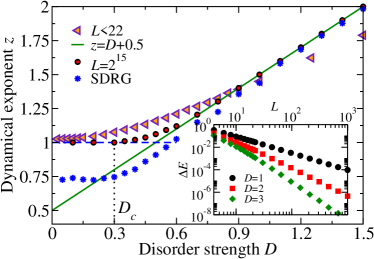
Figure 3: (Color online) Comparison of the dynamical critical exponent for the $\Delta=0$ case computed by exact diagonalizations of small chains ($L<22$), of very large chains ($L=2^{15}$), and via the SDRG method ($L=10^{6}$). Inset: The finite-size gap for different system sizes where the corrections to scaling are clear. Error bars are about the same size as symbols.

As can be guessed from Figs. 1 and 2, due to the available small system sizes, finite-size corrections to the scaling of Eq. (7) are not negligible. We expect $\Delta E\sim L^{-z}\left(1+AL^{-\omega}\right)$, where the constants $A$ and the exponent $\omega$ (which were not calculated) take care of the leading correction to scaling. In order to better see them, we plot in Fig. 3 the exponent $z$ for the anisotropy $\Delta=0$, since bigger lattice sizes can be reached. The results for large chains ($L=2^{15}$) are reproduced from Ref. Hoyos et al., 2011 and the finite-size effects are negligible. The inset shows the finite-size gaps for many system sizes up to $L=10^{3}$. For disorder strength $D=2$ and $3$ it becomes clear that corrections to scaling exist for smaller chains.

Notice that, for $\Delta\geq 0$, our results strongly suggest that $z$ is $\Delta$ independent (see Fig. 2). For $\Delta<0$, we see a small dependence. However, due to the strong finite-size effects, we cannot exclude the possibility of $z$ also being $\Delta$ independent for those negative values.

As we shall see in Secs. IV and V, the entanglement properties and the SDRG analysis also suggest this $\Delta$ independence.

IV The Rényi entanglement entropies and the Shannon mutual information

In this section we numerically compute the Rényi entanglement entropy $S_{n}\left(x,L\right)$ and the Shannon mutual information $I\left(x,L\right)$ of subsystems of size $x$ of an $L$-site XXZ quantum chain. We restrict ourselves to the density matrix formed by the ground state eigenfunction.

We verify that for $D<D_{c}$ these quantities show the same asymptotic behavior as occurs in the clean model [see Eq. (2)]. This is not a surprise since, as discussed in Sec. III, they share the same critical universality class.

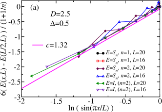
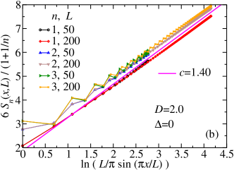
Figure 4: (Color online) Entanglement measures for the correlated disordered XXZ quantum spin chain with (a) anisotropy $\Delta=0.5$ and disorder $D=2.5$ and for (b) anisotropy $\Delta=0$ and disorder $D=2.0$ for several indices $n$ and lattice sizes $L$. Entanglement is measured by the Rényi entanglement entropy $S_{n}$ ($n=1,\,2,\mbox{ and }3$) and by the Shannon mutual information $I$. Data are averaged over $10^{3}$ disorder realizations and the lines are guides to the eyes.

Surprisingly, even for $D>D_{c}$ the finite-size scaling behavior of $S_{n}\left(x,L\right)$ and $I\left(x,L\right)$ are the same as in the clean system. The difference is only in the prefactor “effective central charge.” This is illustrated in Fig. 4, where we plot $S_{n}\left(x,L\right)$ for two values of anisotropies and disorder strengths: $\Delta=1/2$ and $D=2.5$ [panel (a)] and $\Delta=0$ and $D=2.0$ [panel (b)]. Several values of $n$ and length sizes $L$ are shown in the same plot. As can be clearly seen, apart from small oscillations in $S_{n>1}$, all data seems to collapse in a single universal curve. This means that $S_{n}\left(x,L\right)$ and $I\left(x,L\right)$ share the same asymptotic finite-size scaling function as conformally invariant quantum chains [see Eq. (2)], although there is no conformal invariance for those random systems.

The straight solid line is the linear fit for $4\leq x\leq L/2$, from which we extract the effective central charge $c$ values: $1.32$ and $1.40$, for $D=2.5$, $\Delta=0.5$ and $D=2.0$, $\Delta=0$, respectively.

Interestingly, the Shannon mutual information $I$ in Fig. 4(a) has the same asymptotic behavior of $S_{n=2}$.

The Shannon entropy ${\rm Sh}(x,L)$ and consequently the mutual information $I(x,L)$ are, in general, basis-dependent quantities in contrast with the Rényi entanglement entropy which is basis independent. In Fig. 4(a) we computed $I(x,L)$ in the $S^{z}$-basis. Universal behavior for $I(x,L)$ in the conformally invariant systems happens only when the ground state is expressed in the so-called conformal basis that corresponds in the case of the clean XXZ model to the $S^{z}$ and $S^{x}$ bases Alcaraz and Rajabpour (2014). Although we did not compute $I(x,L)$ for our correlated random system using the $S^{x}$ basis, we do not expect any different behavior in this basis.

It is worth mentioning that $I\left(x,L\right)$ does not display the oscillatory parity effect of $S_{2}\left(x,L\right)$, which implies they are indeed different quantities with different subleading terms.

Finally, the fact that we have a straight line even for small subsystem sizes is in contrast to the uncorrelated case, where there is a crossover subsystem size $\xi$ separating the behavior of the clean and disordered systems. This is in agreement with the absence of a crossover length in the correlated disorder case as seen in Sec. III.

In the remainder of this Section, we further explore two other aspects of our numerical results: (i) the prefactor $c_{D}^{{\rm eff}}(1+1/n)/6$ and $c_{D}^{{\rm eff}}/4$ of the leading terms of $S_{n}$ and $I$, respectively, and (ii) the functional dependence of the scaling function with the chord length $\frac{L}{\pi}\sin\frac{\pi x}{L}$.

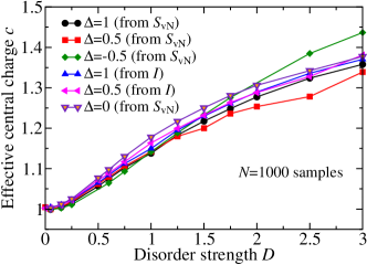
Figure 5: (Color online) The effective central charge as a function of disorder strength $D$ obtained from the von Neumann entanglement entropy $S_{{\rm vN}}$ and from the Shannon mutual information $I$ for various anisotropies $\Delta$. For $\Delta\neq 0$, these values are effective ones due to the system finite size. For extremely large systems, these values crossover to $c_{{\rm IRFP}}^{{\rm eff}}=\ln 2$ (see Sec. V).

For spin chains governed by infinite-randomness fixed points, it is easy to show that the Rényi entanglement entropy $S_{n}\sim\frac{1}{3}c_{{\rm IRFP}}^{{\rm eff}}\ln x$ for any $n$ and $1\ll x\ll L$; i.e., the numerical prefactor $c_{{\rm IRFP}}^{{\rm eff}}$ does not depend on $n$ (see Appendix A). The fact that our spin chains with correlated disorder do not follow this prediction is another indication that the ground state is not a collection of “random singlets.” As already discussed, our numerical results indicate that the leading term has the same dependence on $n$ as conformally invariant systems. In order to check the dependence of $c_{D}^{{\rm eff}}$ with $\Delta$ we plot in Fig. 5 $c_{D}^{{\rm eff}}$ as a function of $D$ for various values of $\Delta$ and for the lattice sizes $L=14,\,16,\,18$, and $20$. The data are averaged $10^{3}$ disorder realizations. Analogously to what happens with the critical dynamical exponent $z$, the effective central charge exhibits quite small variations with the anisotropy $\Delta$. Since we used only relatively small lattice sizes, and we notice the strong statistical fluctuations (especially for higher $D$), it is then plausible to expect that $c_{D}^{{\rm eff}}$ does not depend on $\Delta$, being only a function of $D$.

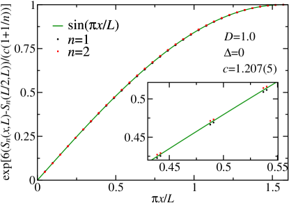
Figure 6: (Color online) The scaling function $f_{L}^{D}\left(x\right)$ measured by using the Rényi entropies $S_{1}$ and $S_{2}$ [see Eq. (8)] for chains of anisotropy $\Delta=0$ and lattice size $L=2^{10}$ averaged over $145\,000$ samples.

The chord length is another hallmark of finite-size scaling functions of conformally invariant systems. It is intriguing that our numerical results are consistent with a scaling function that is also the chord length $f_{L}^{{\rm CFT}}\left(x\right)=\frac{L}{\pi}\sin\left(\frac{\pi}{L}x\right)$. Since this may inspire new analytical insights in those correlated disorder systems, we are now going to verify this statement with higher precision in the case of the Rényi entanglement entropy. We are restricted to the $\Delta=0$ case since we can deal with quite long chains, via a mapping to a free fermion system. In these long chains, we neglect the subleading terms in Eq. (2). In Fig. 6, we plot

$$\frac{L}{\pi}f_{L}^{D}\left(x\right)=\exp\left(6\frac{S_{n}\left(x,L\right)-S_{n}\left(L/2,L\right)}{c_{D}^{{\rm eff}}\left(1+1/n\right)}\right),$$ (8)

as a function of $\frac{\pi x}{L}$, for $n=1$ and $n=2$ and lattice size $L=2^{10}$. The data are averaged over $145\,000$ disorder realizations. We observe a clear agreement with the sine function (continuous green line) $\sin\left(\frac{\pi x}{L}\right)$, implying the leading chord length $f_{L}^{{\rm CFT}}$ dependence for the finite-size scaling functions in our correlated random systems.

In the inset, we zoom in on the region where the curves most largely disagree. Close inspection indicates that the tiny deviations from $\sin\left(\pi x/L\right)$ are due to the imprecision (although small) of the effective central charge value $c_{D}^{{\rm eff}}=1.207(5)$. This may be attributed to the systematic error induced by the non-leading terms in Eq. (2). We also tried to fit the data using other trial functions compatible with the symmetry of $S_{n}$, namely, $f_{1}=\sin\left(\pi x/L\right)+A\sin^{3}\left(\pi x/L\right)$ and $f_{2}=\sin\left(\pi x/L\right)+B\sin\left(3\pi x/L\right)$. The best fit gives $\left(A,B\right)=\left(-1.2,-1.1\right)\times 10^{-3}$ and $\left(-1.5,-1.3\right)\times 10^{-3}$ for $n=1$ and $2$, respectively, which can be taken as zero within our numerical accuracy. Thus, the chord length is likely the scaling function of $S_{n}$.

Moreover, as usually happens in conformally invariant systems, we would like to verify if this same scaling function $f_{L}^{{\rm CFT}}$ also gives the leading behavior for other quantities such as the average transversal spin-spin correlation function $C^{zz}(x,L)=\overline{\left\langle S_{i}^{z}S_{i+x}^{z}\right\rangle}$.

In order to show this, we recall that, to leading order,

$$C^{zz}(x,L)=-\left[Lg\left(x/L\right)\right]^{-\eta_{z}},$$

for $x$ odd. For $x$ even, $C^{zz}=0$. Here, $g\left(z\right)$ is a positive periodic function of unity period and $g(z+1/2)=g(1/2-z)$; and $\eta_{z}$ is the leading decay exponent. Indeed, for the clean system, it is well known Lieb et al. (1961) that

$$C^{zz}(x,L)=-\left(\pi f_{L}^{{\rm CFT}}\left(x\right)\right)^{-2},$$

i.e., the decay exponent $\eta_{z}=2$ and the periodic function is a simple sine. The same universal exponent $\eta_{z}=2$ happens in the uncorrelated disorder case Hoyos et al. (2007) $C^{zz}\sim-1/(12x^{2})$ for $1\ll x\ll L$. Unfortunately, the function $g(z)$ is unknown in this case.

We plot in Fig. 7 $C^{zz}(x,L)\times\left(f_{L}^{{\rm CFT}}\left(x\right)\right)^{2}$ as a function of $\sin\frac{\pi x}{L}$, for several values of the disorder strength $D$ and for lattice sizes $L=200,\,400,\,800$, and $1600$. The fact that this combination saturates to a constant for $x\gtrsim x_{{\rm min}}(L)$ indicates that the chord length, for all the considered values of $D$, is the finite-size scaling function for our correlated disorder case. For $x\lesssim x_{{\rm min}}(L)$, finite-size corrections to scaling are expected [notice $x_{{\rm min}}(L\rightarrow\infty)\rightarrow 0$]. This is in contrast with the uncorrelated disorder case, as shown (for comparison) in Fig. 7. It is clear in this case that the chord length is not the finite-size scaling function. This is not a surprise since it is already known that the finite-size scaling function of the entanglement entropies $S_{n}$ is not a simple sine Fagotti et al. (2011). Furthermore, we also verified that the scaling function appearing in $S_{n}$ found in Ref. Fagotti et al., 2011 is not the scaling function appearing in $C^{zz}$. Namely, a fitting for the periodic function $g(z)$ in the asymptotic region $\sin(\pi z)>1/2$ and for $L=800$ is given by

$$g(z)=\frac{1}{\pi}\sum_{n=1}^{4}A_{2n-1}\sin((2n-1)\pi z),$$

with $A_{1}=1.038$, $A_{3}=0.040$, $A_{5}=-0.007$, and $A_{7}=-0.003$, with similar results for $L=1\,600$.

The fact that the chord length $f_{L}^{{\rm CFT}}$ is the scaling function for both the entropies and the correlation function in our correlated disorder case is an additional resemblance to the long-distance behavior of conformally invariant systems. Actually, for $D<D_{c}$, even the prefactor of the correlation seems to be the same as the one of the clean system (see the dashed line in Fig. 7 and compare with the case $D=0.2<D_{c}$).

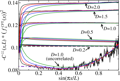
Figure 7: (Color online) The transversal spin-spin correlation function for various disorder strengths $D=0.2$, $0.5$, $1.0$, $1.5$, and $2.0$ (as indicated) and lattice sizes $L=200$ (green), $400$ (blue), $800$ (red), and $1600$ (black). For comparison, we also plot $C^{zz}$ for the clean system (dashed line) and for the system with uncorrelated disorder with $D=1.0$ (bottommost curves). Notice the stronger fluctuations in this latter case. The dotted-dashed line is the fitting curve for the uncorrelated case in the region $\sin(\pi x/L)>1/2$ (see text). In all cases, the data are averaged over $10^{6}$ different disorder configurations, except for $L=1\,600$ where the number of samples used is $50\,000$. Error bars are not shown for clarity but are of the order of the data fluctuations.

Finally, we comment on the remarkable similarity between the Shannon mutual information and the Rényi entanglement entropy $S_{2}$ as shown in Fig. 4(a). As recently conjectured, the Shannon mutual information behaves like $S_{2}$ in the long-length limit $1\ll x\ll L$ for clean conformally invariant systems Alcaraz and Rajabpour (2013, 2014); Stéphan (2014). It is remarkable that the same similarity is present in our random spin chain. Evidently, one would also like to compare with the mutual information of spin chains governed by infinite-randomness fixed points. Although $I$ is not computed in the literature, this is a simple task which we accomplish in Appendix A. It turns out that $I\left(x,L\right)=S_{n}\left(x,L\right)$ for random singlet states (and for any $n$), which trivially agrees with the conjecture.

In summary, our numerical results indicate that the ground states of quantum chains governed by this line of fixed points have entanglement properties which are similar to those of conformally invariant ground states. This is an unexpected result which certainly deserves further attention in order to understand the complete generality of the results derived from conformally invariant systems.

V Strong-disorder renormalization group

In this section we provide a strong-disorder renormalization-group (SDRG) treatment of our correlated disorder spin chain in Eq. (5). The main purpose is to understand the role of the anisotropy in our line of finite-disorder fixed points. As shown below, this gives us support to the conjecture that the anisotropy is an irrelevant parameter in the region $-1<\Delta\leq 1$. In addition, this treatment also sheds some light on the nature of the ground state wave function of our system.

The SDRG method Ma et al. (1979); Dasgupta and Ma (1980); Bhatt and Lee (1982) gives us an appropriate machinery for studying infinite-randomness fixed points. It gives us an asymptotically exact description of the low-energy eigenlevels of the system Iglói and Monthus (2005). In addition, it has also been used to describe systems governed by finite-disorder fixed points, giving us plausible results Westerberg et al. (1997); Yusuf and Yang (2003); Hoyos and Miranda (2004). Up to now, a precise comparison of the SDRG results derived in this latter case with exact results is still lacking. In the present section, we are going to present such a comparison for our correlated random system.

The main idea of the SDRG method is to integrate out local high-energy degrees of freedom, renormalizing the remaining ones via perturbation theory. In this way the low-energy physics is accessed, provided that the perturbative procedure becomes more accurate along the renormalization-group flow.

Here, our purpose is to study the perfectly correlated case of Eq. (5). However, because new operators arise along the RG flow, it is more convenient to expand the parameter space and consider the more general Hamiltonian

$$H=\sum_{i}H_{i}=\sum_{i}J_{i}\left(S_{i}^{x}S_{i+1}^{x}+S_{i}^{y}S_{i+1}^{y}+\Delta_{i}S_{i}^{z}S_{i+1}^{z}\right).$$ (9)

There are two differences from Eq. (5): (i) the anisotropy $\Delta_{i}$ is now a random variable, and not fixed as before, and is correlated with the coupling constants $J_{i}$ as we are going to explain below. (ii) The coupling constants $J_{i}$ are not perfectly correlated (as $J_{1},J_{1},J_{3},J_{3},\dots$).

The local energy scale is $\epsilon_{i}=J_{i}(1+\Delta_{i})/2$ which is the local gap of $H_{i}$. As the SDRG method is an energy-based method, what is relevant is the correlation among the random scales $\epsilon_{i}$. For this reason, we quantify the correlation among the random scales of the system via the quantity

$$\alpha=\alpha_{{\rm even,odd}}+\alpha_{{\rm odd,even}},$$ (10)

where $\alpha_{{\rm even,odd}}=(\left\langle\epsilon_{2i}\epsilon_{2i+1}\right\rangle-\epsilon_{{\rm odd}}\epsilon_{{\rm even}})/\sigma_{{\rm odd}}\sigma_{{\rm even}}$, $\epsilon_{{\rm x}}=\overline{\epsilon_{{\rm x}}}$ is the disorder average over ${\rm x}={\rm even,odd}$ sites, and $\sigma_{{\rm x}}^{2}=\overline{\epsilon_{{\rm x}}^{2}}-\overline{\epsilon_{{\rm x}}}^{2}$ is the variance. Likewise $\alpha_{{\rm odd,even}}=(\left\langle\epsilon_{2i-1}\epsilon_{2i}\right\rangle-\epsilon_{{\rm odd}}\epsilon_{{\rm even}})/\sigma_{{\rm odd}}\sigma_{{\rm even}}$ measures the correlation between the odd-numbered sites and their rightmost neighbors. Notice that for uncorrelated disorder $\alpha=0$, whereas $\alpha=1$ for the case of perfectly correlated disorder, as in Eq. (5).

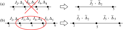
Figure 8: (Color online) Decimation procedure for (a) uncorrelated and (b) correlated disorder.

It is instructive to review the SDRG procedure applied to the uncorrelated case $\alpha=0$ in the region $-1<\Delta_{i}\leq 1$ Fisher (1994). One searches for the greatest local energy scale $\Omega=\max\{\epsilon_{i}\}$, say $\Omega=\epsilon_{3}$, and then treats $H_{2}+H_{4}$ as a perturbation to $H_{3}$. As a result, spins $S_{3}$ and $S_{4}$ become locked in a singlet and the neighboring spins $S_{2}$ and $S_{5}$ experience an effective interaction given by $\tilde{H}_{2}=\tilde{J}_{2}\left(S_{2}^{x}S_{5}^{x}+S_{2}^{y}S_{5}^{y}+\tilde{\Delta}_{2}S_{2}^{z}S_{5}^{z}\right)$, where the renormalized couplings are $\tilde{J}_{2}=\frac{J_{2}J_{4}}{J_{3}\left(1+\Delta_{3}\right)}$ and $\tilde{\Delta}_{2}=\frac{1}{2}\Delta_{2}\Delta_{4}\left(1+\Delta_{3}\right)$ [see Fig. 8(a)]. Within this procedure Fisher (1994), it was shown that the fixed point is of infinite-disorder type, i.e., $\sigma_{\epsilon}/\overline{\epsilon}\rightarrow\infty$ when $\Omega\rightarrow 0$ (which provides a posteriori justification of the perturbative procedure), and that the anisotropy always renormalizes to zero (except for the isotropic case $\Delta_{i}=1$). This conclusion is valid whenever $-\frac{1}{2}<\Delta_{i}<1$. For $-1<\Delta_{i}<-\frac{1}{2}$, the same conclusion applies only if the bare disorder of the system is sufficiently strong. For $\left|\Delta_{i}\right|>1$, the long-range order of the system is not changed by disorder, i.e., the system keeps its ferromagnetic (for $\Delta_{i}<-1$) or antiferromagnetic (for $\Delta_{i}>1$) Ising character. The entanglement properties are thus similar to that of the clean system in which a finite correlation length exists, i.e., it obeys the usual area law.

Clearly, this SDRG procedure cannot be applied for correlated disorder $\alpha\neq 0$ because the assumption that $\Omega=\epsilon_{3}\gg\epsilon_{2,4}$ fails. This can be circumvented by choosing a larger spin cluster that also includes all the possible strong local couplings. Because the correlations in Eq. (5) are short ranged, such a cluster will be composed of three spins. For instance if $\Omega=\epsilon_{3}$, then spins $S_{3}$ and $S_{4}$ belong to that triad of spins. In order to decide if the third spin is either $S_{2}$ or $S_{5},$ we look for $\max\{\epsilon_{2},\epsilon_{4}\}$. In fact, a more precise measure of the local energy scale $\varepsilon_{i}$ is the mass gap of $H_{i}+H_{i+1}$. Thus, we redefine the SDRG cutoff energy scale to $\Omega=\max\{\varepsilon_{i}\}$. This identifies the strongly correlated spin triad. Once the energy cutoff is found, say $\Omega=\varepsilon_{3}$, the next step is to treat $H_{2}+H_{5}$ as a perturbation to $H_{3}+H_{4}$. Since the ground state of $H_{3}+H_{4}$ is a doublet it can be recast as an effective spin-1/2 degree of freedom. Thus, projecting $H_{2}+H_{5}$ onto this doublet is equivalent to replacing spins $S_{3}$, $S_{4}$, and $S_{5}$ by an effective spin $\tilde{S}_{5}$, which is connected to $S_{2}$ and $S_{6}$ via effective couplings as depicted in Fig. 8(b) (see details in Appendix B).

Notice the fundamental difference between these two approaches. For uncorrelated disorder, the ground state is always a random singlet state regardless of the details of the random variables. For correlated disorder, on the other hand, the effective spin $\tilde{S}_{5}$ has strong correlations with the original spins $S_{3}$, $S_{4}$, and $S_{5}$ if $\epsilon_{3}\approx\epsilon_{4}$. Therefore, this correlation can be transmitted away to the rest of the chain when $\tilde{S}_{5}$ is decimated out in a later stage of the SDRG flow. In the end, correlations among the original spins can be greatly enhanced and the ground state can be fundamentally different from the random singlet state. This is indeed the case as shown below.

Unfortunately, the effective couplings $\tilde{J}_{i}$ and $\tilde{\Delta}_{i}$ cannot be worked out analytically in an easy way (see Appendix B). We have implemented the SDRG decimation procedure numerically. However, before presenting our numerical results, it is instructive to consider some limiting cases of interest which can shed some light about the renormalized system.

Let us first consider the case of perfectly correlated disorder $J_{4}=J_{3}$ and $\Delta_{4}=\Delta_{3}$ [which is exactly the one we are interested in Eq. (5)]. Projecting $H_{2}+H_{5}$ onto the ground state of $H_{3}+H_{4}$ yields an effective Hamiltonian as depicted in Fig. 8(b) with

$$\tilde{J}_{i}=\frac{2J_{i}}{\sqrt{8+\Delta_{3}^{2}}}\mbox{ and }\tilde{\Delta}_{i}=\left(\frac{\Delta_{3}+\sqrt{8+\Delta_{3}^{2}}}{4}\right)\Delta_{i}.$$ (11)

Two aspects of the renormalized couplings are noteworthy. (i) Even if the bare system has perfectly correlated disorder as in Eq. (5) (i.e., the couplings are $J_{1}J_{1}J_{3}J_{3}J_{5}J_{5}\dots$), the renormalized system does not display such a feature: $J_{1}\tilde{J}_{1}\tilde{J}_{5}J_{5}\dots$. This is the reason why we have expanded the parameter’s space of our original Hamiltonian. (ii) The renormalized anisotropies are smaller than the original ones. This suggests that, as for the uncorrelated disorder case, the anisotropy renormalizes to zero. Naturally, both points (i) and (ii) have been extensively tested as shown below.

Another case that can be studied exactly is the free-fermion one $\Delta_{i}=0$ (see Appendix A). Here, the $\Delta_{i}$ remains zero along the SDRG flow and the renormalized coupling constants in Fig. 8(b) are

$$\tilde{J}_{2}=\frac{J_{2}J_{4}}{\sqrt{J_{3}^{2}+J_{4}^{2}}}\mbox{ and }\tilde{J}_{5}=\frac{J_{3}J_{5}}{\sqrt{J_{3}^{2}+J_{4}^{2}}}.$$ (12)

Again, the perfect correlations of the original chain $J_{1}J_{1}J_{3}J_{3}J_{5}J_{5}\dots$ are lost after just the first decimation.

Finally, the third case in which the decimation rules can be worked out analytically is the isotropic $SU(2)$ one where $\Delta_{i}=1$. As in the free-fermion case, the anisotropy does not change and is fixed at $\tilde{\Delta}_{i}=1$. The effective coupling constants are

$$\tilde{J}_{2}=\left(\frac{2J_{4}-J_{3}+\gamma}{3\gamma}\right)J_{2}\mbox{ and }\tilde{J}_{5}=\left(\frac{2J_{3}-J_{4}+\gamma}{3\gamma}\right)J_{5},$$ (13)

with $\gamma=\sqrt{J_{3}^{2}-J_{3}J_{4}+J_{4}^{2}}$. Again, as in the previous cases, the perfect correlation is lost along the SDRG flow.

The lessons learned from this little digression (and confirmed by our numerical study below) are (i) the fixed points are either $\tilde{\Delta}_{i}=0$ or $\tilde{\Delta}_{i}=1$ and (ii) perfect correlation on the energy scales is lost during the SDRG flow. Lesson (ii) raises an important question. If perfect correlation is lost, does the system flow to a totally uncorrelated fixed point which would be of infinite-randomness type? As shown below, this is indeed the case except for the free-fermion case $\Delta_{i}=0$.

We now report our numerical study of the SDRG method on our random spin chains with correlated disorder Eq. (5). The SDRG decimation procedure (as described above) is depicted in Fig. 8(b). As the energy scale $\Omega$ is lowered, we keep track of the renormalized values of the disorder correlation measure $\tilde{\alpha}$ and the mean $\left\langle\tilde{\Delta}\right\rangle$ anisotropy, together with its variance $\sigma_{\tilde{\Delta}}^{2}$, and the length scale $\xi=\rho^{-1}$ which is also the inverse of density $\rho=L/n_{\Omega}$ ($n_{\Omega}$ being the number of spin clusters at the energy scale $\Omega$). In all of our runs, the chain is decimated until the system is reduced to 20 spin clusters.

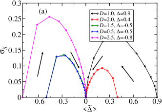
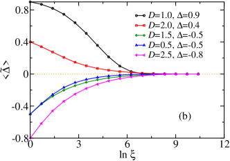
Figure 9: (Color online) The anisotropy along the SDRG flow for various disorder parameters $D$ and initial conditions $\Delta$, for the case of perfectly correlated disorder $\alpha=1$. In panel (a) the standard deviation $\sigma_{\tilde{\Delta}}$ is plotted as a function of the average $\left\langle\tilde{\Delta}\right\rangle$, with the arrows indicating the direction of the SDRG flow. In panel (b) $\left\langle\tilde{\Delta}\right\rangle$ is plotted as a function of the SDRG length scale $\xi$. The lines are guides to the eyes and the data are averaged over only $10$ disorder realizations of a large lattice size of $L=10^{6}$.

We show in Fig. 9 that the anisotropy is an irrelevant perturbation at the critical line $-1<\Delta<1$, i.e., the low-energy physics is governed by the free-fermion fixed point $\tilde{\Delta}=0$. In this figure, only a few disorder realizations are enough for a reasonable precision due to the very large lattice size used.

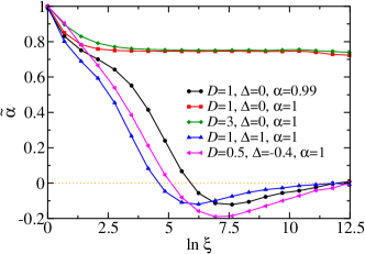
Figure 10: (Color online) Disorder correlation along the SDRG flow for various disorder strengths $D$ and anisotropies $\Delta$. The correlation parameter $\alpha$ is plotted as a function of the SDRG length scale $\xi$. Data are averaged over $1\,000$ disorder realizations of large chains of size $10^{7}$. Lines are guides to the eyes.

The effective disorder correlations of our system are shown in Fig. 10. We plot the correlation measure of the renormalized disorder variables $\tilde{\alpha}$ along the SDRG flow, as a function of the length scale $\xi$. As can be seen, except for the case where $\Delta=0$ and perfectly correlated disorder $\alpha=1$, the disorder correlation of the renormalized coupling constants $\tilde{\alpha}\rightarrow 0$ at the final stages of the flow. This means that the true fixed point is the one of the uncorrelated disorder case which is of infinite-randomness type. Notice, however, that the correlation does not vanish fast. In the RG language, this means a long incursion of the flow near the fixed point of the system with perfectly correlated disorder. As a consequence, the physics of relatively small system sizes is governed by the finite-disorder fixed point. This is compatible with the results we presented in Secs. III and IV for the $\Delta\neq 0$ cases.

How can we explain the different behaviors between the cases $\Delta\neq 0$ and $\Delta=0$? Actually, we have solid arguments in favor of a vanishing random mass term only in the special case $\alpha=1$ and $\Delta=0$ Hoyos et al. (2011). The results of Secs. III and IV, derived for small lattice sizes $L\leq 20$, are compatible with a similar vanishing random mass for $\Delta\neq 0$. However, as the SDRG results reveal (see Fig. 10), there is a relatively large crossover length above which random mass becomes relevant.

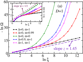
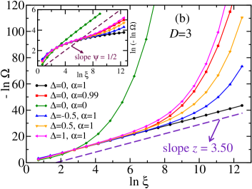
Figure 11: (Color online) The relation between the energy $\Omega$ and the length $\xi$ scales for the disorder strengths (a) $D=1$ and (b) $D=3$ and various anisotropies $\Delta$ and correlation $\alpha$. Dashed lines are the best fits for the case $\Delta=0$ and $\alpha=1$ restricted to $\ln\xi\geq 7$. Inset: The same as in the main plot with the logarithmic value of the vertical axis. Dashed lines are the corresponding theoretical slopes for infinite-randomness physics.

In order to test this interpretation, we investigate the system dispersion relation by plotting the energy scale $\Omega$ as a function of the length scale $\xi$. For conventional dynamics, a power-law scaling $\Omega\sim\xi^{-z}$ is expected, compatible with a finite-disorder fixed point (absence of random mass). On the other hand, for an infinite-randomness fixed point (presence of random mass) Fisher (1994), an activated dynamical scaling takes place in which $\ln\Omega\sim-\xi^{\psi}$, with universal tunneling exponent $\psi=\frac{1}{2}$. Therefore, for $\Delta\neq 0$ (irrespective whether disorder is perfectly correlated or not), or for $\Delta=0$ but $\alpha\neq 1$ (disorder not perfectly correlated), we expect a conventional power-law scaling in the earlier stages of the SDRG flow, and activated dynamics after a crossover. This is indeed the observed scenario as shown in Fig. 11. Notice that, for small length scales, a power-law scaling $\Omega\sim\xi^{-z}$ takes place. This regime is governed by the “unstable” fixed point which has no random mass. In this transient regime, the critical dynamical exponent does not depend on the anisotropy $\Delta$, in agreement with the results obtained by exact diagonalization in Sec. III.

Interestingly, the SDRG method here presented can be quantitatively compared with exact results. The dynamical exponent $z$, obtained from the fits in Fig. 11, is plotted in Fig. 3 together with the expected exact value. Two features are noteworthy. (i) For weak disorder $D<D_{c}$ the SDRG method indicates a universal finite-disorder fixed point. Because the corresponding $z_{{\rm SDRG}}$ is less than $z_{{\rm clean}}=1$, we interpret that the correct fixed point is the one of the clean system. This is a consequence of the delocalized modes (spinons) are energetically favorable against the localized ones obtained by the SDRG method; i.e., the delocalized modes are the true low-energy modes. (ii) The dynamical critical exponent $z_{{\rm SDRG}}$ is quantitatively close to the exact one even for small $z,$ say $z\approx 1.5$. Thus, even though the SDRG is only justifiable at strong disorder ($z\gg 1$), it already gives relatively accurate results even for moderate $z$. In addition, notice that the $z_{{\rm SDRG}}$ is always smaller than $z$. We interpret this in the following manner. Let us suppose we could untangle the localized and delocalized modes coming from the limits of weak and strong disorder, respectively. Clearly, in the way the SDRG method is formulated, only the localized modes are captured, namely, resonances of a triad of strongly coupled spin clusters. However, these are not the true modes of the system. There are certain aspects of the delocalized theory that are not taken into account. For instance, our spin-triad resonance may interact with spinons. This interaction would further lower the energy of the modes, which would correspond to a larger dynamical exponent. Hence $z$ is greater than or equal to $z_{{\rm clean}}=1$ and $z_{{\rm SDRG}}$.

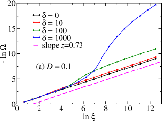
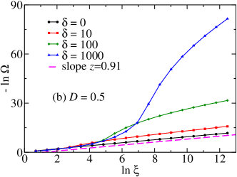
Figure 12: (Color online) The scaling relation between energy $\Omega$ and length $\xi$ for the $\Delta=0$ chain with the even coupling constants spatially shifted by an amount $\delta$ and disorder strengths (a) $D=0.1$ and (b) $D=0.5$. Dashed lines are the fits for the unshifted case for $\ln\xi\geq 7$.

Let us now briefly discuss on the possibility that the observed finite random mass (in the case $\Delta\neq 0$) is just an artificial product of the inexactness of the SDRG method. One could argue that our decimation procedure does not preserve locally the disorder correlation, and therefore random mass is introduced even for $\Delta=0$. This would imply that the nearly perfect match between $z$ and $z_{{\rm SDRG}}$ is just a coincidence. The important detail that must be kept in mind is that the random mass is a coarse-grained concept, and hence the local constraint $\tilde{J}_{2i-1}=\tilde{J}_{2i}$ is not necessary.

We believe that indeed the absence of the random mass is captured by the SDRG method even when it is not present in the short length scale. This reasoning is based on the following study. Instead of using the correlated chain in Eq. (5) where the coupling constants at sites $2i-1$ and $2i$ are correlated ($\dots J_{1}J_{1}J_{3}J_{3}J_{5}J_{5}\dots$), we shift the correlated couplings by an integer $\delta>2$ such that the sequence of couplings is now $\dots J_{1}J_{1+\delta}J_{3}J_{3+\delta}J_{5}J_{5+\delta}\dots$. In this way, since $J_{i}$ has no correlation with $J_{i+\delta}$ for $\delta>2$, there is no cancellation of the random mass term at sites $i$ and $i+1$. The absence of random mass would be observed only at length scales $\xi\gg\delta$, where the condition $\prod J_{2i}=\prod J_{2i-1}$ becomes approximately fulfilled. This is indeed what is verified in the energy-length dispersion relation as shown in Fig. 12. For $\xi<\delta$, the system “sees” local random masses and the scaling is activated. Only for $\xi\gg\delta,$ does the true asymptotic regime take place where the dynamical critical exponent is finite and equals the one of the unshifted ($\delta=0$) chain. Even the correlation between the effective coupling constants becomes finite, as plotted in Fig. 13. For $\delta>2$, the correlation $\alpha$ is initially zero, and after coarse-graining it builds up as in the $\delta=0$ case. For large $\delta$, the crossover from the activated to the power-law dynamical scaling is very slow, taking over on a large range of length scales $\xi.$

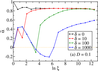
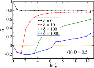
Figure 13: (Color online) The correlation measure $\tilde{\alpha}$ for the $\Delta=0$ chain with the even coupling constants shifted by an amount $\delta$ and disorder strengths (a) $D=0.1$ and (b) $D=0.5$.

Thus, it is plausible to conclude that our SDRG decimation procedure does not introduce random masses in the $\Delta\neq 0$ case, as happens for the $\Delta=0$ case.

Finally, in order to conclude this section, let us discuss on a possible generalization of the $c$ theorem Zamolodchikov (1986), which states that if RG flow between two conformally invariant fixed points $a$ and $b$ is in the direction $a\rightarrow b$, then the corresponding central charges are such that $c_{a}\geq c_{b}$. In the earlier years of the study of entanglement properties of random spin chains, the quest for an effective $c$ theorem fostered intense research Refael and Moore (2007, 2004); Santachiara (2006); Fidkowski et al. (2008). It turned out that such generalization was proven impossible for spin chains governed by infinite-randomness fixed points since violations were observed Santachiara (2006); Fidkowski et al. (2008). It is worth asking if such violation also happens in our correlated disordered case.

Probing the SDRG flow (as described in Sec. V) for the XX model ($\Delta_{i}=0$) described by the Hamiltonian (9), we conclude that there is no violation of the $c$ theorem. This conclusion stems from the following reasoning. Consider the SDRG flow in the $D$-$\alpha$ parameter space, where the disorder strength $D$ is defined in Eq. (6) and the correlation in the disorder variables $\alpha$ is defined in Eq. (10). As shown in Fig. 10, any perturbation away from the perfectly correlated disorder drives the flow towards the uncorrelated disorder case. Thus, the line of finite-disorder fixed points is unstable towards the infinite-disorder fixed point along the $\alpha$ direction. As shown in Ref. Hoyos et al., 2011 (see also Fig. 2), weak disorder is perturbatively relevant in the perfectly correlated case ($\alpha=1$), hence the RG flow goes from the finite-disorder fixed points towards the clean fixed point; i.e., the line of fixed points is unstable along the $D$ direction as well. Finally, it is well know that the clean fixed point is unstable towards the infinite-disorder fixed point along the $D$ direction (as long as $\alpha\neq 1$). As $c_{{\rm IFRP}}^{{\rm eff}}=\ln 2<c_{{\rm clean}}=1<c_{D}^{{\rm eff}}$, we conclude that the SDRG flow is compatible with an “effective” $c$ theorem. At the line of finite-disorder fixed points, one may inquire if there is any violation of this effective theorem. Notice that there is no flow among these fixed points since their basin of attractions is null.

VI Conclusion and discussions

We have studied the critical spin-1/2 XXZ chain with short-range correlated disorder. Due to absence of the random mass, this system has the interesting property of realizing a line of finite-disorder fixed points tuned by the disorder strength. Such mass absence is asserted by the local correlation $J_{2i}=J_{2i-1}$ in the free-fermion case $\Delta=0$. In the general case $\Delta\neq 0$, the random mass is present although its magnitude is quite small. Thus, the line of fixed points governs the physics in the intermediate-energy regime. Here, we did not consider the question of whether it is possible to devise local correlations among the disorder variables of the microscopic model in Eq. (5) for $\Delta\neq 0$ in order to ensure an effective theory free of random mass.

As it is well known, the violation of the area law of the entanglement entropy of critical systems happens for both clean and disordered systems. The most studied disordered chains are those with uncorrelated disorder which realizes infinite-randomness fixed points. In this case, differently from the clean systems which are usually conformally invariant, the $n$-Rényi entanglement entropies are independent of the index $n$, being equal to the Shannon entanglement entropy.

In this paper, we performed an extensive study of the entanglement properties of ground states of quantum chains governed by finite-disorder fixed points. Surprisingly, we obtained quite different results from those of infinite-disorder fixed points. In contrast, the leading finite-size behaviors show striking resemblances with those of the clean conformally invariant systems, even though the critical random system under consideration is not conformally invariant. These resemblances are (a) the same $n$ dependence occurs in the Rényi entanglement entropy $S_{n}$, (b) the same periodic scaling function $f_{L}^{{\rm CFT}}(x)=\frac{L}{\pi}\sin\left(\frac{\pi x}{L}\right)$ is applicable for the entanglement properties as well as for the spin-spin correlation functions, and (c) the Shannon mutual information $I(x)$ and the Rényi entanglement entropy $S_{2}(x)$ share the same leading behavior as conjectured for conformally invariant systems.

From the results in the literature up to now, the logarithmic behavior of the entanglement entropies seems to be a general feature of one-dimensional critical systems regardless of being disordered or not. However, the periodic finite-size scaling function $f_{L}^{{\rm CFT}}(x)$ appearing in the argument of this logarithmic dependence (also in the correlation functions) is normally expected to be a signature of the underlying conformal field theory governing the long-distance physics of the system. Our results give us two possibilities: either this behavior is a consequence of more general assumptions than conformal invariance, or there is some emerging effective conformal symmetry in those correlated disordered systems which is not obvious. This latter possibility is quite intriguing since the dynamical critical exponent $z>1$. Emerging symmetries in critical random systems have been recently reported Quito et al. (2015), but are still poorly understood.

This paper also gives us the first extension of the conjecture stating that $S_{2}(x)$ and $I(x)$, in conformally invariant systems and computed on certain special basis, share the same leading asymptotic behavior for large systems and subsystem sizes. It would be quite interesting to test this conjecture in other disordered systems.

Appendix A Entanglement in random singlet phases

For completeness, we derive the Shannon mutual information and the Rényi entanglement entropy for the random singlet state of the antiferromagnetic spin-1/2 chain.

It has been shown Hoyos and Rigolin (2006); Hoyos et al. (2007); Tran and Bonesteel (2011); Pouranvari and Yang (2013) that the random singlet state is well approximated by a collection of singlet pairs

$$\left|\psi\right\rangle=\bigotimes_{i=1}^{L/2}\left|s_{i}\right\rangle=\bigotimes_{a=1}^{N_{a}}\left|s_{a}\right\rangle\bigotimes_{b=1}^{N_{b}}\left|s_{b}\right\rangle\bigotimes_{ab=1}^{N_{ab}}\left|s_{ab}\right\rangle,$$ (14)

where $\left|s_{i}\right\rangle=\frac{1}{\sqrt{2}}\left(\left|+-\right\rangle-\left|-+\right\rangle\right)$ is the singlet state of the $i$-th singlet pair. We divide these singlets into three categories: those in which (a) both spins belong to region ${\cal A}$, (b) both spins belong to region ${\cal B}$, and (ab) one of the spins belongs to region ${\cal A}$ while the other one belongs to ${\cal B}$. They are denoted respectively by $\left|s_{a}\right\rangle$, $\left|s_{b}\right\rangle$ and $\left|s_{ab}\right\rangle$, and there are $N_{a}$, $N_{b}$ and $N_{ab}$ of each. The constraint is that $N_{a}+N_{b}+N_{ab}=L/2$.

The reduced density matrix $\rho_{A}$ can be easily computed as

$$\rho_{A}=\bigotimes_{a}\left|s_{a}\right\rangle\left\langle s_{a}\right|\bigotimes_{ab}\frac{1}{2}\left(\left|+\right\rangle\left\langle+\right|+\left|-\right\rangle\left\langle-\right|\right).$$ (15)

Thus, the nonvanishing eigenvalues of $\rho_{A}$ come from the ab singlets. There are $2^{N_{ab}}$ degenerate eigenvalues equal to $\lambda_{i}=2^{-N_{ab}}$, and therefore, the $n$-Rényi entanglement entropy is

$$S_{n}=\frac{\ln\left(\sum_{i}\lambda_{i}^{n}\right)}{1-n}=\frac{\ln\left(2^{N_{ab}-nN_{ab}}\right)}{1-n}=N_{ab}\ln 2,$$ (16)

which does not depend on the index $n$.

The Shannon mutual information can be computed in a similar way. Let us start with the Shannon entropy of the entire system. The random-singlet state in Eq. (14) has $2^{L/2}$ different configurations, all of them occurring with the same probability $2^{-L/2}$. Therefore ${\rm Sh}\left({\cal A}\cup{\cal B}\right)=-2^{L/2}\times 2^{-L/2}\ln 2^{-L/2}=\frac{L}{2}\ln 2$. Now, let us compute the Shannon entropy for subsystem ${\cal A}$. It is easy to see that all possible configurations will appear with the same probability. Thus, our task is to compute only the number of different configurations. Due to the $N_{a}$ singlets inside region ${\cal A}$, there will be a contribution of $2^{N_{a}}$ configurations. Moreover, we have to take into account the $N_{ab}$ singlets which are shared by both subsystems. Each such pair has one spin in subsystem ${\cal A}$ which will appear with equal probability in the $\left|+\right\rangle$ and $\left|-\right\rangle$ states. Thus, the total number of configurations is $2^{N_{a}+N_{ab}}$. Likewise for the subsystem ${\cal B}$, the total number of configurations is $2^{N_{b}+N_{ab}}$. We are now in position to compute the Shannon mutual information:

$$I={\rm Sh}\left({\cal A}\right)+{\rm Sh}\left({\cal B}\right)-{\rm Sh}\left({\cal A}\cup{\cal B}\right)=N_{ab}\ln 2,$$ (17)

where we have used $N_{a}+N_{b}+N_{ab}=L/2$. Therefore, the leading term of the Shannon mutual information equals the leading term of the Rényi entanglement entropy for all $n$ for random-singlet states. Notice that this result does not depend exactly on how the singlets are distributed on the chain. This is important only to relate $N_{ab}$ with $x$. Moreover, this result can be generalized to any spin $S$. One needs only to replace $\ln 2$ by $\ln 2S+1$.

Finally, we mention that the number of spin singlets belonging to both subsystems ${\cal A}$ and ${\cal B}$ can be computed with the methods in the literature Refael and Moore (2004); Hoyos et al. (2007). Let $x$ be the ${\cal A}$ subsystem size. It is found that for $1\ll x\ll L$, $N_{ab}=\frac{1}{3}\ln x$. With this, one recovers the known result that $S_{n}=\frac{1}{3}c_{{\rm RS}}\ln x$, with the universal prefactor $c_{{\rm RS}}=\ln 2$.

Appendix B Three-spins SDRG

We wish to treat $H^{\prime}$ as a perturbation to $H$ where

$$H= J_{3}\left(\frac{S_{3}^{+}S_{4}^{-}+{\rm h.c.}}{2}+\Delta_{3}S_{3}^{z}S_{4}^{z}\right)$$

$$+J_{4}\left(\frac{S_{4}^{+}S_{5}^{-}+{\rm h.c.}}{2}+\Delta_{4}S_{4}^{z}S_{5}^{z}\right),$$

and

$$H^{\prime}= J_{2}\left(\frac{S_{2}^{+}S_{3}^{-}+{\rm h.c.}}{2}+\Delta_{2}S_{2}^{z}S_{3}^{z}\right)$$

$$+J_{5}\left(\frac{S_{5}^{+}S_{6}^{-}+{\rm h.c.}}{2}+\Delta_{5}S_{5}^{z}S_{6}^{z}\right).$$

We then need to diagonalize $H$. Due to conservation of the total $z$ magnetization $S^{z}$, the eigenvalue problem for this Hamiltonian can be reduced by solving a single $3\times 3$ matrix. Two eigenvectors follow straightforwardly (corresponding to $S^{z}=\pm\frac{3}{2}$): $\left|+++\right\rangle$ and $\left|---\right\rangle$, being degenerate with eigenenergy $E_{4}=\frac{1}{4}\left(J_{3}\Delta_{3}+J_{4}\Delta_{4}\right)$. There are three eigenvectors obtained from the $S^{z}=+\frac{1}{2}$ sector whose corresponding matrix is

$$\mathbb{M}=\frac{1}{2}\left(\begin{array}[]{ccc}\frac{+J_{3}\Delta_{3}-J_{4}\Delta_{4}}{2}&J_{4}&0\\ J_{4}&\frac{-J_{3}\Delta_{3}-J_{4}\Delta_{4}}{2}&J_{3}\\ 0&J_{3}&\frac{-J_{3}\Delta_{3}+J_{4}\Delta_{4}}{2}\end{array}\right),$$

where the order $\left|++-\right\rangle$, $\left|+-+\right\rangle$, and $\left|-++\right\rangle$ was used. The same result is obtained in the $S^{z}=-\frac{1}{2}$ sector.

Since the system is antiferromagnetic ($-1<\Delta_{2,3}\leq 1$), the ground states are doubly degenerate and belong to the sectors $S^{z}=\pm\frac{1}{2}$. The eigenvalues of $\mathbb{M}$ are the roots of a cubic polynomial, which we denote by $E_{1,2,3}$ with $E_{1}<E_{2,3,4}$. The degenerate ground states are $\left|\tilde{+}\right\rangle=a_{1}\left|++-\right\rangle+a_{2}\left|+-+\right\rangle+a_{3}\left|-++\right\rangle$ and $\left|\tilde{-}\right\rangle=-a_{1}\left|--+\right\rangle-a_{2}\left|-+-\right\rangle-a_{3}\left|+--\right\rangle$, with $a_{i}\in\Re$. Once the doublet is obtained, our task is to project $H^{\prime}$ onto the doublet $\left|\tilde{\pm}\right\rangle$; i.e., we need to project $S_{3}$ and $S_{5}$ onto the doublet $\left|\tilde{\pm}\right\rangle$:

$$S_{i}^{\alpha}\rightarrow\left(\begin{array}[]{cc}\left\langle\tilde{+}\left|S_{i}^{\alpha}\right|\tilde{+}\right\rangle&\left\langle\tilde{+}\left|S_{i}^{\alpha}\right|\tilde{-}\right\rangle\\ \left\langle\tilde{-}\left|S_{i}^{\alpha}\right|\tilde{+}\right\rangle&\left\langle\tilde{-}\left|S_{i}^{\alpha}\right|\tilde{-}\right\rangle\end{array}\right).$$

We then find that $S_{3}^{+}\rightarrow-2a_{1}a_{2}\tilde{S}_{5}^{+}$, $S_{5}^{+}\rightarrow-2a_{3}a_{2}\tilde{S}_{5}^{+}$, $S_{3}^{z}\rightarrow\frac{1}{2}\left(a_{1}^{2}+a_{2}^{2}-a_{3}^{3}\right)\tilde{S}_{5}^{z}$, $S_{5}^{z}\rightarrow\frac{1}{2}\left(-a_{1}^{2}+a_{2}^{2}+a_{3}^{3}\right)\tilde{S}_{5}^{z}$, where $\tilde{S}_{5}^{+}=\left(\begin{array}[]{cc}0&1\\ 0&0\end{array}\right)$ and $\tilde{S}_{5}^{z}=\frac{1}{2}\left(\begin{array}[]{cc}1&0\\ 0&-1\end{array}\right)$. Thus, we arrive at the effective Hamiltonian

$$\tilde{H}^{\prime}= \tilde{J}_{2}\left(\frac{S_{2}^{+}\tilde{S}_{5}^{-}+{\rm h.c.}}{2}+\tilde{\Delta}_{2}S_{2}^{z}\tilde{S}_{5}^{z}\right)$$

$$+\tilde{J}_{5}\left(\frac{\tilde{S}_{5}^{+}S_{6}^{+}+{\rm h.c.}}{2}+\tilde{\Delta}_{5}\tilde{S}_{5}^{z}S_{6}^{z}\right),$$ (18)

with the renormalized couplings

$$\tilde{J}_{2}=-2a_{1}a_{2}J_{2},\quad\tilde{J}_{5}=-2a_{2}a_{3}J_{5},$$

$$\tilde{\Delta}_{2}=\frac{-a_{1}^{2}-a_{2}^{2}+a_{3}^{2}}{2a_{1}a_{2}}\Delta_{2},\quad\tilde{\Delta}_{5}=\frac{a_{1}^{2}-a_{2}^{2}-a_{3}^{2}}{2a_{2}a_{3}}\Delta_{5}.$$

This decimation procedure is depicted in Fig. 8(b). Notice that a global signal can be gauged out for all couplings since we can choose a harmless global factor in $\left|\tilde{-}\right\rangle$.

Unfortunately, we could not solve the coefficients $a_{i}$ analytically for the ground state in the generic case. Nevertheless, three important limiting cases can be worked out analytically: (i) perfect correlation $J_{4}=J_{3}$ and $\Delta_{4}=\Delta_{3}$, (ii) free fermions $\Delta_{i}=0$, and (ii) isotropic Heisenberg $\Delta_{i}=1$.

For the special case where $J_{4}=J_{3}$ and $\Delta_{4}=\Delta_{3}$, the eigenvalues of $\mathbb{M}$ are $E_{1,2}=-\frac{1}{4}J_{3}\left(\Delta_{3}\pm\sqrt{8+\Delta_{3}^{2}}\right)$ and $E_{3}=0$, and the ground states are $\left|\tilde{+}\right\rangle=J_{3}\left|++-\right\rangle+2E_{1}\left|+-+\right\rangle+J_{3}\left|-++\right\rangle$ and $\left|\tilde{-}\right\rangle=-J_{3}\left|--+\right\rangle-2E_{1}\left|-+-\right\rangle-J_{3}\left|+--\right\rangle$ which can be recast as an effective spin-1/2 degree of freedom (notice $\left\langle\tilde{+}\left|S^{z}\right|\tilde{+}\right\rangle=-\left\langle\tilde{-}\left|S^{z}\right|\tilde{-}\right\rangle=1/2$). The projected operators are $S_{3}^{+}=S_{5}^{+}\rightarrow\frac{2}{\sqrt{8+\Delta_{3}^{2}}}\tilde{S}_{5}^{+}$ and $S_{3}^{z}=S_{5}^{z}\rightarrow\left(1+\frac{\Delta_{3}}{\sqrt{8+\Delta_{3}^{2}}}\right)\tilde{S}_{5}^{z}$, and, consequently, the effective couplings are

$$\tilde{J}_{i}=\frac{2}{\sqrt{8+\Delta_{3}^{2}}}J_{i}\mbox{ and }\tilde{\Delta}_{i}=\left(\frac{\Delta_{3}+\sqrt{8+\Delta_{3}^{2}}}{4}\right)\Delta_{i}.$$

In the free fermion case $\Delta_{i}=0$, the eigenvalues of $\mathbb{M}$ are $E_{1,2}=\mp\frac{1}{2}\sqrt{J_{3}^{2}+J_{4}^{2}}$ and $E_{3}=0$. Hence, the doublet is $\left|\tilde{+}\right\rangle=J_{4}\left|++-\right\rangle+2E_{1}\left|+-+\right\rangle+J_{3}\left|-++\right\rangle$ and $\left|\tilde{-}\right\rangle=-J_{4}\left|--+\right\rangle-2E_{1}\left|-+-\right\rangle-J_{3}\left|+--\right\rangle$, which yields the projections $S_{3}^{+}\rightarrow\frac{J_{4}}{\sqrt{J_{3}^{2}+J_{4}^{2}}}\tilde{S}_{5}^{+}$ and $S_{5}^{+}\rightarrow\frac{J_{3}}{\sqrt{J_{3}^{2}+J_{4}^{2}}}\tilde{S}_{5}^{+}$. We then arrive at the effective Hamiltonian

$$\tilde{H}^{\prime}=\tilde{J}_{2}\left(\frac{S_{2}^{+}\tilde{S}_{5}^{-}+{\rm h.c.}}{2}\right)+\tilde{J}_{5}\left(\frac{\tilde{S}_{5}^{+}S_{6}^{+}+{\rm h.c.}}{2}\right),$$

with

$$\tilde{J}_{2}=\frac{J_{2}J_{4}}{\sqrt{J_{3}^{2}+J_{4}^{2}}}\mbox{ and }\tilde{J}_{5}=\frac{J_{3}J_{5}}{\sqrt{J_{3}^{2}+J_{4}^{2}}}.$$

Finally, we consider the SU(2)-symmetric case $\Delta_{i}=1$. Here, the eigenenergies are $E_{1,2}=-\frac{1}{4}\left(J_{3}+J_{4}\pm 2\gamma\right)$ (with $\gamma=\sqrt{J_{3}^{2}-J_{3}J_{4}+J_{4}^{2}}$), and $E_{3}=E_{4}=\frac{1}{4}\left(J_{3}+J_{4}\right)$ and the corresponding ground state is $\left|\tilde{+}\right\rangle=\left(-J_{3}+J_{4}+\gamma\right)\left|++-\right\rangle-\left(J_{4}+\gamma\right)\left|+-+\right\rangle+J_{3}\left|-++\right\rangle$. Thus, the renormalized couplings are

$$\tilde{J}_{2}=\left(\frac{2J_{4}-J_{3}+\gamma}{3\gamma}\right)J_{2}\mbox{ and }\tilde{J}_{5}=\left(\frac{2J_{3}-J_{4}+\gamma}{3\gamma}\right)J_{5}.$$

As expected, $\tilde{\Delta}_{2,5}=\Delta_{2,5}=1$ which preserves the SU(2) symmetry.

References

- Holzhey et al. (1994) C. Holzhey, F. Larsen, and F. Wilczek, Nuclear Physics B 424, 443 (1994).
- Calabrese and Cardy (2004) P. Calabrese and J. Cardy, Journal of Statistical Mechanics: Theory and Experiment 2004, P06002 (2004).
- Calabrese et al. (2010) P. Calabrese, M. Campostrini, F. Essler, and B. Nienhuis, Phys. Rev. Lett. 104, 095701 (2010).
- Xavier and Alcaraz (2011) J. C. Xavier and F. C. Alcaraz, Phys. Rev. B 83, 214425 (2011).
- Alcaraz and Rajabpour (2013) F. C. Alcaraz and M. A. Rajabpour, Phys. Rev. Lett. 111, 017201 (2013).
- Alcaraz and Rajabpour (2014) F. C. Alcaraz and M. A. Rajabpour, Phys. Rev. B 90, 075132 (2014).
- Stéphan (2014) J.-M. Stéphan, Phys. Rev. B 90, 045424 (2014).
- Fisher (1994) D. S. Fisher, Phys. Rev. B 50, 3799 (1994).
- Fisher (1995) D. S. Fisher, Phys. Rev. B 51, 6411 (1995).
- Refael and Moore (2004) G. Refael and J. E. Moore, Phys. Rev. Lett. 93, 260602 (2004).
- Laflorencie (2005) N. Laflorencie, Phys. Rev. B 72, 140408 (2005).
- Hoyos and Rigolin (2006) J. A. Hoyos and G. Rigolin, Phys. Rev. A 74, 062324 (2006).
- Santachiara (2006) R. Santachiara, Journal of Statistical Mechanics: Theory and Experiment 2006, L06002 (2006).
- Hoyos et al. (2007) J. A. Hoyos, A. P. Vieira, N. Laflorencie, and E. Miranda, Phys. Rev. B 76, 174425 (2007).
- Bonesteel and Yang (2007) N. E. Bonesteel and K. Yang, Phys. Rev. Lett. 99, 140405 (2007).
- Fidkowski et al. (2008) L. Fidkowski, G. Refael, N. E. Bonesteel, and J. E. Moore, Phys. Rev. B 78, 224204 (2008).
- Fagotti et al. (2011) M. Fagotti, P. Calabrese, and J. E. Moore, Phys. Rev. B 83, 045110 (2011).
- Tran and Bonesteel (2011) H. Tran and N. E. Bonesteel, Phys. Rev. B 84, 144420 (2011).
- Pouranvari and Yang (2013) M. Pouranvari and K. Yang, Phys. Rev. B 88, 075123 (2013).
- Ramírez et al. (2014) G. Ramírez, J. Rodríguez-Laguna, and G. Sierra, Journal of Statistical Mechanics: Theory and Experiment 2014, P07003 (2014).
- Ma et al. (1979) S.-k. Ma, C. Dasgupta, and C.-k. Hu, Phys. Rev. Lett. 43, 1434 (1979).
- Dasgupta and Ma (1980) C. Dasgupta and S.-k. Ma, Phys. Rev. B 22, 1305 (1980).
- Bhatt and Lee (1982) R. N. Bhatt and P. A. Lee, Phys. Rev. Lett. 48, 344 (1982).
- Nguyen et al. (1996) T. N. Nguyen, P. A. Lee, and H.-C. z. Loye, Science 271, 489 (1996).
- Irons et al. (2000) S. H. Irons, T. D. Sangrey, K. M. Beauchamp, M. D. Smith, and H.-C. zur Loye, Phys. Rev. B 61, 11594 (2000).
- Koteswararao et al. (2010) B. Koteswararao, A. V. Mahajan, L. K. Alexander, and J. Bobroff, Journal of Physics: Condensed Matter 22, 035601 (2010).
- Westerberg et al. (1997) E. Westerberg, A. Furusaki, M. Sigrist, and P. A. Lee, Phys. Rev. B 55, 12578 (1997).
- Yusuf and Yang (2003) E. Yusuf and K. Yang, Phys. Rev. B 68, 024425 (2003).
- Hoyos and Miranda (2004) J. A. Hoyos and E. Miranda, Phys. Rev. B 69, 214411 (2004).
- Lavarélo et al. (2013) A. Lavarélo, G. Roux, and N. Laflorencie, Phys. Rev. B 88, 134420 (2013).
- Binosi et al. (2007) D. Binosi, G. De Chiara, S. Montangero, and A. Recati, Phys. Rev. B 76, 140405 (2007).
- Hoyos et al. (2011) J. A. Hoyos, N. Laflorencie, A. P. Vieira, and T. Vojta, Europhys. Lett. 93, 30004 (2011).
- Pfeuty (1979) P. Pfeuty, Phys. Lett. A 72, 245 (1979).
- Laflorencie et al. (2004) N. Laflorencie, H. Rieger, A. W. Sandvik, and P. Henelius, Phys. Rev. B 70, 054430 (2004).
- Lieb et al. (1961) E. Lieb, T. Schultz, and D. Mattis, Ann. Phys. 16, 407 (1961).
- Iglói and Monthus (2005) F. Iglói and C. Monthus, Phys. Rep. 412, 277 (2005).
- Zamolodchikov (1986) A. B. Zamolodchikov, JETP Lett. 43, 730 (1986).
- Refael and Moore (2007) G. Refael and J. E. Moore, Phys. Rev. B 76, 024419 (2007).
- Quito et al. (2015) V. L. Quito, J. A. Hoyos, and E. Miranda, Phys. Rev. Lett. 115, 167201 (2015).