Baryogenesis in the Zee-Babu model with arbitrary $\xi$ gauge

Abstract

We consider the baryogenesis picture in the Zee-Babu model. Our analysis shows that electroweak phase transition (EWPT) in the model is a first-order phase transition at the $100$ GeV scale, its strength ranges from 1 to 4.15 and the masses of charged Higgs boson are smaller than $300$ GeV. The EWPT is strengthened by only the new bosons and this strength is enhanced by arbitrary $\xi$ gauge. However, the $\xi$ gauge does not break the first-order EWPT or, in other words, the $\xi$ gauge is not the cause of the EWPT. This leads to the fact that the calculation of EWPT in Landau gauge is enough; and the latter may provide baryon-number violation (B-violation) necessary for baryogenesis in the relationship with nonequilibrium physics in the early universe.

Keywords: Spontaneous breaking of gauge symmetries, Extensions of electroweak Higgs sector, Particle-theory models (Early Universe)

I INTRODUCTION

Physics, at present, has entered into a new period, on the understanding the early Universe. In that context, Cosmology and Particle Physics are on the same way. Being as a central issue of cosmology and particle physics, at present the baryon asymmetry is an interesting problem. If we could explain this problem, we can understand the true nature of the smallest elements and reveal a lot about an imbalances matter-antimatter from the early Universe.

The electroweak baryogenesis (EWBG) is a way to explaining the baryon asymmetry of the Universe (BAU) in the early Universe, associating with Sakharov conditions, which are B, C, $CP$ violations, and deviation from thermal equilibrium sakharov . These conditions can be satisfied when the EWPT must be a strongly first-order phase transition. Because that not only leads to thermal imbalance mkn , but also makes a connection between B and $CP$ violation via nonequilibrium physics ckn .

The EWPT has been investigated in the standard model (SM) Ref.mkn ; SME ; michela as well as its various extended versions BSM ; majorana ; thdm ; ESMCO ; elptdm ; phonglongvan ; SMS ; dssm ; munusm ; lr ; singlet ; mssm1 ; twostep ; 1101.4665 . For the SM, although the EWPT strength is larger than unity at the electroweak scale, the mass of the Higgs boson must be less than $125$ GeV mkn ; SME ; michela ; so the EWBG requires new physics beyond the SM at the weak scale BSM .

Many extensions such as the two-Higgs-boublet model, the reduced minimal 3-3-1 model, the economical 3-3-1 model or the Minimal Supersymmetric Standard Model, have a strongly first-order EWPT and the new sources of CP violation, which are necessary to account for the BAU; triggers for the first-order EWPT in these models are heavy bosons or Dark Matter candidates majorana ; thdm ; ESMCO ; elptdm ; phonglongvan ; singlet ; mssm1 ; twostep ; chiang3 . However, most research of the EWPT are the Landau gauge. Recently gauge invariant also made important contributions in the EWPT as researching in Refs.1101.4665 ; Arefe .

The quantity of sphaleron rate admitting to B violation rate, has been calculated in the SM in Refs.mkn ; SME ; michela and in the reduced minimal 3-3-1 model in Ref. phonglongvan . In addition, by using nonperturbative lattice simulations, a powerful framework and set of analytic and numerical tools have been developed in Refs. SME ; michela .

The Zee-Babu (ZB) model is one of the simplest extensions of the SM which has some interesting features zeebabu . Due to its simplicity, in this work, we have considered the EWPT and sphaleron rate in the ZB model.

In the ZB model, two extra charged scalars $h^{\pm}$ and $k^{\pm\pm}$ are added to the Higgs potential. The kind of new scalars can play an important role in the early Universe. As shown in zeebabu ; bzee , they can also be a reason for tiny mass of neutrinos through two loop or three loop corrections. One important property of these particles which will be shown in this paper, is that they can be triggers for the first-order phase transition.

In order to drive a gauge dependent effective potential at one-loop level, in this paper we will use a direct method which is different from those used in Refs. 1101.4665 ; Arefe . This paper is organized as follows. In Sec. II we give a short review of the ZB model and we drive an effective potential which has a contribution from heavy scalars and the $\xi$ gauge at one-loop level. In Sec. III, we find the mass range of charged scalar particles by a first-order phase transition condition. Finally, Sec. IV is devoted to constraints on the mass of the charged Higgs boson. In Sec. V we summarize and describe outlooks.

II EFFECTIVE POTENTIAL IN THE ZEE-BABU MODEL

In the ZB model, by adding two charged scalar fields $h^{\pm}$ and $k^{\pm\pm}$ zeebabu , the Lagrangian becomes

$$\mathcal{L} = L_{SM}+f_{ab}\overline{\psi_{aL}^{c}}\psi_{bL}h^{+}+h_{ab}^{{}^{\prime}}\overline{l_{aR}^{c}}l_{bR}k^{++}+V(\phi,h,k)$$ (1)

$$+(D_{\mu}h^{+})^{\dagger}(D^{\mu}h^{+})+(D_{\mu}k^{++})^{\dagger}(D^{\mu}k^{++})+H.c$$

In the model, the Higgs potential contains more four couplings between $h^{\pm}$ or $k^{\pm\pm}$ and neutral Higgs boson zeebabu :

$$V(\phi,h,k) = \mu^{2}\phi^{\dagger}\phi+u^{2}_{1}{|{h}|}^{2}+u_{2}^{2}{|{k}|}^{2}+\lambda(\phi^{\dagger}\phi)^{2}+\lambda_{h}{|{h}|}^{4}+\lambda_{k}{|{k}|}^{4}$$ (2)

$$+\lambda_{hk}{|{h}|}^{2}{|{k}|}^{2}+2p^{2}{|{h}|}^{2}\phi^{\dagger}\phi+2q^{2}{|{k}|}^{2}\phi^{\dagger}\phi+(\mu_{hk}h^{2}k^{++}+H.c)\,,$$

where

$$\phi=\left(\begin{array}[]{c}\rho^{+}\\ \rho^{0}\end{array}\right)$$ (3)

and $\rho^{0}$ has a vacuum expectation value (VEV)

$$\rho^{0}=\frac{1}{\sqrt{2}}\left(v_{0}+\sigma+i\zeta\right)\,.$$ (4)

The masses of $h^{\pm}$ and $k^{{\pm\pm}}$ are given by

$$m^{2}_{h^{\pm}} = p^{2}v^{2}_{0}+u^{2}_{1},$$

$$m^{2}_{{k^{\pm\pm}}} = q^{2}v^{2}_{0}+u^{2}_{2}.$$ (5)

Diagonalizing matrices in the kinetic components of the Higgs potential and retaining Goldstone bosons, we obtain

$$\begin{aligned} m_{H}^{2}(v_{0})&=-\mu^{2}+3\lambda v^{2}_{0}\,,\\ m_{G}^{2}(v_{0})&=-\mu^{2}+\lambda v^{2}_{0}\,,\\ \end{aligned}\begin{aligned} m_{Z}^{2}(v_{0})&=\textstyle\frac{1}{4}(g^{2}+g^{\prime 2})v^{2}_{0}=a^{2}v^{2}_{0}\,,\\ m_{W}^{2}(v_{0})&=\textstyle\frac{1}{4}g^{2}v^{2}_{0}=b^{2}v^{2}_{0}\,.\\ \end{aligned}$$ (6)

II.1 EFFECTIVE POTENTIAL WITH LANDAU GAUGE

From Eq. (1), ignoring Goldstone bosons, we obtain an effective potential with contributions of $h^{\pm}$ and $k^{{\pm\pm}}$ in the Landau gauge:

$$V_{eff}(v) = V_{0}(v)+\frac{3}{64\pi^{2}}\left(m_{Z}^{4}(v)ln\frac{m_{Z}^{2}(v)}{Q^{2}}+2m_{W}^{4}(v)ln\dfrac{m_{W}^{2}(v)}{Q^{2}}-4m_{t}^{4}(v)ln\dfrac{m_{t}^{2}(v)}{Q^{2}}\right)$$ (7)

$$+ \frac{1}{64\pi^{2}}\left(2m_{h^{\pm}}^{4}(v)ln\dfrac{m_{h^{\pm}}^{2}(v)}{Q^{2}}+2m_{k^{\pm\pm}}^{4}(v){ln}\dfrac{m_{k^{\pm\pm}}^{2}(v)}{Q^{2}}+m_{H}^{4}(v)ln\dfrac{m_{H}^{2}(v)}{Q^{2}}\right)$$

$$+ \frac{3T^{4}}{4\pi^{2}}\left\{F_{-}(\frac{m_{Z}(v)}{T})+F_{-}(\frac{m_{W}(v)}{T})+4F_{+}(\frac{m_{t}(v)}{T})\right\}$$

$$+ \frac{T^{4}}{4\pi^{2}}\left\{2{F}_{-}(\frac{m_{h^{\pm}}(v)}{T})+2{F}_{-}(\frac{m_{k^{\pm\pm}}(v)}{T})+{F}_{-}(\frac{{m}_{H}(v)}{T})\right\}\,,$$

where $v_{\rho}$ is a variable changing with temperature, and at $T=0$, $v_{\rho}\equiv v_{0}=246$ GeV. Here

$$F_{\pm}\left(\dfrac{m_{\phi}}{T}\right) = \int_{0}^{\dfrac{m_{\phi}}{T}}\alpha J_{\mp}^{1}(\alpha,0)d\alpha,$$

$$J_{\mp}^{1}(\alpha,0) = 2\int_{\alpha}^{\infty}\dfrac{(x^{2}-\alpha^{2})^{\frac{1}{2}}}{e^{x}\mp 1}dx.$$

II.2 EFFECTIVE POTENTIAL WITH $\xi$ GAUGE

It is known that in high levels, the contribution of Goldstone boson cannot be ignored. Therefore, we must consider an effective potential in arbitrary $\xi$ gauge given by

$$\mathcal{V}_{1}^{T=0}(v) = \frac{1}{4(4\pi)^{2}}(m_{H}^{2})^{2}\big{[}\ln(\textstyle\frac{m_{H}^{2}}{Q^{2}})-\frac{3}{2}\displaystyle\big{]}+\frac{1}{4(4\pi)^{2}}(m_{h^{\pm}}^{2})^{2}\big{[}\ln(\textstyle\frac{m_{h^{\pm}}^{2}}{Q^{2}})-\frac{3}{2}\displaystyle\big{]}$$ (8)

$$+\frac{1}{4(4\pi)^{2}}(m_{k^{\pm\pm}}^{2})^{2}\big{[}\ln(\textstyle\frac{m_{{k^{\pm\pm}}}^{2}}{Q^{2}})-\frac{3}{2}\displaystyle\big{]}+\frac{2\times 1}{4(4\pi)^{2}}(m_{G}^{2}+\xi m_{W}^{2})^{2}\big{[}\ln(\textstyle\frac{m_{G}^{2}+\xi m_{W}^{2}}{Q^{2}})-\frac{3}{2}\displaystyle\big{]}$$

$$+\frac{1}{4(4\pi)^{2}}(m_{G}^{2}+\xi m_{Z}^{2})^{2}\big{[}\ln(\textstyle\frac{m_{G}^{2}+\xi m_{Z}^{2}}{Q^{2}})-\frac{3}{2}\displaystyle\big{]}+\frac{2\times 3}{4(4\pi)^{2}}(m_{W}^{2})^{2}\big{[}\ln(\textstyle\frac{m_{W}^{2}}{Q^{2}})-\frac{5}{6}\displaystyle\big{]}$$

$$+\frac{3}{4(4\pi)^{2}}(m_{Z}^{2})^{2}\big{[}\ln(\textstyle\frac{m_{Z}^{2}}{Q^{2}})-\frac{5}{6}\displaystyle\big{]}-\frac{2\times 1}{4(4\pi)^{2}}(\xi m_{W}^{2})^{2}\big{[}\ln(\textstyle\frac{\xi m_{W}^{2}}{Q^{2}})-\frac{3}{2}\displaystyle\big{]}$$

$$-\frac{1}{4(4\pi)^{2}}(\xi m_{Z}^{2})^{2}\big{[}\ln(\textstyle\frac{\xi m_{Z}^{2}}{Q^{2}})-\frac{3}{2}\displaystyle\big{]}-\text{``free''},$$

and

$$\mathcal{V}^{T\neq 0}_{1}(v,T) = \frac{T^{4}}{2\pi^{2}}\bigg{[}J_{B}\Big{(}\frac{m_{H}^{2}}{T^{2}}\Big{)}+J_{B}\Big{(}\frac{m_{h^{\pm}}^{2}}{T^{2}}\Big{)}+2J_{B}\Big{(}\frac{m_{k^{\pm\pm}}^{2}}{T^{2}}\Big{)}\bigg{]}$$ (9)

$$+\frac{T^{4}}{2\pi^{2}}\bigg{[}2\!\times\!J_{B}\Big{(}\frac{m_{G}^{2}+\xi m_{W}^{2}}{T^{2}}\Big{)}+J_{B}\Big{(}\frac{m_{G}^{2}+\xi m_{Z}^{2}}{T^{2}}\Big{)}\bigg{]}$$

$$+\frac{3T^{4}}{2\pi^{2}}\bigg{[}2\!\times\!J_{B}\Big{(}\frac{m_{W}^{2}}{T^{2}}\Big{)}+J_{B}\Big{(}\frac{m_{Z}^{2}}{T^{4}}\Big{)}+J_{B}\Big{(}\frac{m_{\gamma}^{2}}{T^{4}}\Big{)}\bigg{]}$$

$$-\frac{T^{4}}{2\pi^{2}}\bigg{[}2\!\times\!J_{B}\Big{(}\frac{\xi m_{W}^{2}}{T^{2}}\Big{)}+J_{B}\Big{(}\frac{\xi m_{Z}^{2}}{T^{2}}\Big{)}+J_{B}\Big{(}\frac{\xi m_{\gamma}^{2}}{T^{2}}\Big{)}\bigg{]}-\text{``free''},$$

where “free” represents a free-field subtraction.

III ELECTROWEAK PHASE TRANSITION IN THE ZEE-BABU MODEL

III.1 EWPT in Landau gauge

Ignoring $u_{1}$ and $u_{2}$ in Eq.(II) (i.e., $u_{1}$ and $u_{2}$ are assumed to be very small) and neglecting contributions of Goldstone bosons, we can write the high-temperature expansion of the potential in Eq.(7) as a quartic expression in $v$:

$$V_{eff}(v)=D(T^{2}-T^{2}_{0})v^{2}-ET|v|^{3}+\frac{\lambda_{T}}{4}v^{4},$$ (10)

in which

$$D = \frac{1}{24{v_{0}}^{2}}\left[6m_{W}^{2}(v_{0})+3m_{Z_{1}}^{2}(v_{0})+m_{H}^{2}(v_{0})+2m_{h^{\pm}}^{2}(v_{0})+2m_{k^{\pm\pm}}^{2}(v_{0})+6m_{t}^{2}(v_{0})\right],$$

$$T_{0}^{2} = \frac{1}{D}\left\{\frac{m_{H}^{2}(v_{0})}{4}-\frac{1}{32\pi^{2}v_{0}^{2}}\left(6m_{W}^{4}(v_{0})+3m_{Z_{1}}^{4}(v_{0})+m_{H}^{4}(v_{0})\right.\right.$$

$$\left.\left.\qquad\qquad\qquad\qquad+2m_{h^{\pm}}^{4}(v_{0})+2m_{k^{\pm\pm}}^{4}(v_{0})-12m_{t}^{4}(v_{0})\right)\right\},$$

$$E = \frac{1}{12\pi v_{0}^{3}}\left(6m_{W}^{3}(v_{0})+3m_{Z_{1}}^{3}(v_{0})+m_{H}^{3}(v_{0})+2m_{h^{\pm}}^{3}(v_{0})+2m_{k^{\pm\pm}}^{3}(v_{0})\right),$$ (11)

$$\lambda_{T} = \frac{m_{H}^{2}(v_{0})}{2v_{0}^{2}}\left\{1-\frac{1}{8\pi^{2}v_{0}^{2}(m_{H}^{2}(v_{0}))}\left[6m_{W}^{4}(v_{0})\ln\frac{m_{W}^{2}(v_{0})}{a_{b}T^{2}}\right.\right.$$

$$\qquad\left.\left.+3m_{Z_{1}}^{4}(v_{0})\ln\frac{m_{Z_{1}}^{2}(v_{0})}{a_{b}T^{2}}+m_{H^{0}}^{4}(v_{0})\ln\frac{m_{H^{0}}^{2}(v_{0})}{a_{b}T^{2}}\right.\right.$$

$$\qquad\left.\left.+2m_{k^{\pm\pm}}^{4}(v_{0})\ln\frac{m_{k^{\pm\pm}}^{2}(v_{0})}{a_{b}T^{2}}+2m_{h^{\pm}}^{4}(v_{0})\ln\frac{m_{h^{\pm}}^{2}(v_{0})}{a_{b}T^{2}}-12m_{t}^{4}(v_{0})\ln\frac{m_{t}^{2}(v_{0})}{a_{F}T^{2}}\right]\right\},$$

where $v_{0}$ is the value where the zero-temperature effective potential $V^{0}_{eff}(v)$ gets the minimum. Here, we acquire $V^{0}_{eff}$ from $V_{eff}$ in Eq.(10) by neglecting all terms in the form $F_{\mp}\left(\frac{m}{T}\right)$.

The minimum conditions for $V^{0}_{eff}(v)$ are

$$V^{0}_{eff}(v_{0})=0,\hskip 8.5359pt\frac{\partial V^{0}_{eff}(v)}{\partial v}\Big{|}_{v=v_{0}}=0,\hskip 8.5359pt\frac{\partial^{2}V^{0}_{eff}(v)}{\partial v^{2}}\Big{|}_{v=v_{0}}=\left[m^{2}_{H}(v)\right]\Big{|}_{v=v_{0}}=125^{2}\text{ GeV}^{2}.$$ (12)

We also have the minima of the effective potential in Eq.(10)

$$v=0,\quad v\equiv v_{c}=\frac{2ET_{c}}{\lambda_{T_{c}}},$$ (13)

where $v_{c}$ is the critical VEV of $\phi$ at the broken state, and $T_{c}$ is the critical temperature of phase transition given by

$$T_{c}=\frac{T_{0}}{\sqrt{1-E^{2}/D\lambda_{T_{c}}}}.$$ (14)

Now let us investigate the phase transition strength

$$S=\frac{v_{c}}{T_{c}}=\frac{2E}{\lambda_{T_{c}}}$$ (15)

of this EWPT. In the limit $E\rightarrow 0$, the transition strength tends to zero ($S\rightarrow 0$) and the phase transition is a second-order one. To have a first-order phase transition, we require that the strength is larger or equal to the unit ($S\geq 1$). In Fig. 1, we have plotted the transition strength $S$ as a function of the new charged scalars: $m_{h^{\pm}}$ and $m_{k^{\pm\pm}}$.

According to Ref. 5percent , the accuracy of a high-temperature expansion for the effective potential such as that in Eq. (10) will be better than $5\%$ if $\frac{m_{boson}}{T}<2.2$, where $m_{boson}$ is the relevant boson mass. Therefore, as shown in Fig. 1, for $m_{h^{\pm}}$ and $m_{k^{\pm\pm}}$ being in the $0-350\,\mathrm{GeV}$ range, respectively, the transition strength is in the range $1\leq S<2.4$.

We see that the contribution of $h^{\pm}$ and $k^{\pm\pm}$ are the same. The larger mass of $h^{\pm}$ and $k^{\pm\pm}$, the larger cubic term ($E$) in the effective potential but the strength of phase transition cannot be strong. Because the value of $\lambda$ also increases, so there is a tension between $E$ and $\lambda$ to make the first order phase transition. In addition when the masses of charged Higgs bosons are too large, $T_{0},\lambda$ will be unknown or $S\longrightarrow\infty$.

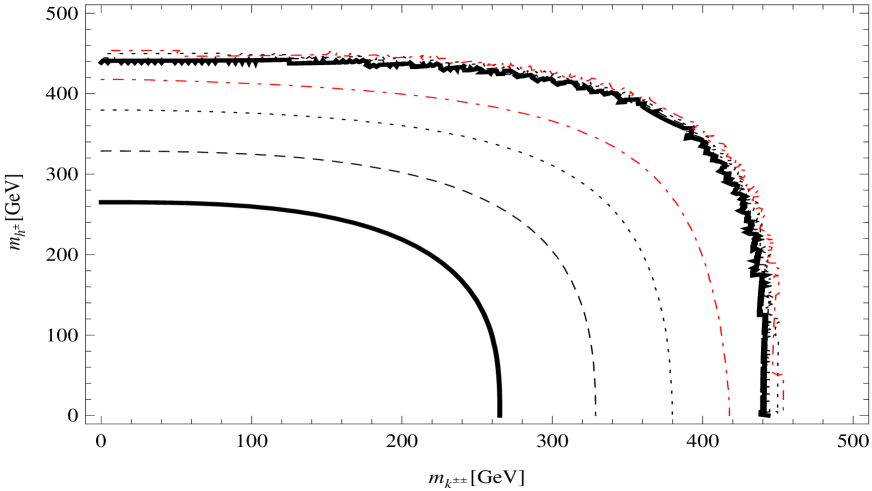
Figure 1: When the solid contour of $S=2E/\lambda_{T_{c}}=1$, the dashed contour: $2E/\lambda_{T_{c}}=1.5$, the dotted contour: $2E/\lambda_{T_{c}}=2$, the dotted-dashed contour: $2E/\lambda_{T_{c}}=2.4$, even and nosmooth contours: $S\longrightarrow\infty$.

III.2 EWPT in $\xi$ gauge

The high-temperature expansions of the potential in Eq.(8) and in Eq.(9) can be rewritten in a like-quartic expression in $v$

$$\mathcal{V} = \left(\mathcal{D}_{1}+\mathcal{D}_{2}+\mathcal{D}_{3}+\mathcal{D}_{4}+\mathcal{B}_{2}\right)v^{2}+\mathcal{B}_{1}v^{3}+\Lambda v^{4}+f(T,u_{1},u_{2},\mu,\xi),$$ (16)

where

$$f(T,u_{1},u_{2},\mu,\xi,v)=\mathcal{C}_{1}+\mathcal{C}_{2},$$ (17)

and

$$\mathcal{D}_{1} = \frac{T^{2}}{24v^{2}_{0}}\left(3m^{2}_{Z}(v_{0})+6m^{2}_{W}(v_{0})+6m^{2}_{t}(v_{0})+2(m^{2}_{h^{\pm}}(v_{0})-u_{1}^{2})+2(m^{2}_{k^{\pm\pm}}(v_{0})-u_{2}^{2})+6\lambda v^{2}_{0}\right)\,,$$

$$\mathcal{D}_{2} = \frac{1}{32v^{2}_{0}\pi^{2}}\left\{3m^{4}_{Z}(v_{0})+6m^{4}_{W}(v_{0})-12m^{4}_{t}(v_{0})+2(m^{2}_{h^{\pm}}(v_{0})-u_{1}^{2})^{2}-8\pi^{2}v^{2}_{0}m^{2}_{H_{0}}\right.$$

$$\quad\left.+2(m^{2}_{k^{\pm\pm}}(v_{0})-u_{2}^{2})^{2}+12v_{0}^{4}\lambda^{2}+2m^{2}_{Z}(v_{0})v^{2}_{0}\lambda\xi+4m^{2}_{W}(v_{0})v^{2}_{0}\lambda\xi\right\},$$

$$\mathcal{D}_{3} = \frac{1}{32\pi^{2}}\left\{2p^{2}u_{1}^{2}\ln\left[\frac{a_{b}T^{2}}{p^{2}v_{0}^{2}+u_{1}^{2}}\right]+2q^{2}u_{2}^{2}\ln\left[\frac{a_{b}T^{2}}{q^{2}v_{0}^{2}+u_{2}^{2}}\right]\right.$$

$$\quad\left.-3\lambda\mu^{2}\ln\left[\frac{a_{b}T^{2}}{3v_{0}^{2}\lambda-\mu^{2}}\right]-\lambda\mu^{2}\ln\left[\frac{a_{b}T^{2}}{v_{0}^{2}\left(\lambda+a^{2}\xi\right)-\mu^{2}}\right]\right.$$

$$\quad\left.-2\lambda\mu^{2}\ln\left[\frac{a_{b}T^{2}}{v_{0}^{2}\left(\lambda+b^{2}\xi\right)-\mu^{2}}\right]-a^{2}\xi\mu^{2}\ln\left[\frac{a_{b}T^{2}}{v_{0}^{2}\left(\lambda+a^{2}\xi\right)-\mu^{2}}\right]\right.$$

$$\quad\left.-2b^{2}\xi\mu^{2}\ln\left[\frac{a_{b}T^{2}}{v_{0}^{2}\left(\lambda+b^{2}\xi\right)-\mu^{2}}\right]\right\}\,,$$

$$\mathcal{D}_{4} = \frac{1}{32\pi^{2}}\left(2p^{2}u_{1}^{2}+2q^{2}u_{2}^{2}-6\lambda\mu^{2}-a^{2}\xi\mu^{2}-2b^{2}\xi\mu^{2}\right)\,,$$

$$\Lambda = \frac{1}{64\pi^{2}}\left\{2p^{4}\ln\left[\frac{a_{b}T^{2}}{u_{1}^{2}+p^{2}v_{0}^{2}}\right]+2q^{4}\ln\left[\frac{a_{b}T^{2}}{u_{2}^{2}+q^{2}v_{0}^{2}}\right]+3a^{4}\ln\left[\frac{a_{b}T^{2}}{a^{2}v_{0}^{2}}\right]+6b^{4}\ln\left[\frac{a_{b}T^{2}}{b^{2}v_{0}^{2}}\right]\right.$$

$$\quad\left.-12k^{4}\ln\left[\frac{a_{F}T^{2}}{k^{2}v_{0}^{2}}\right]+9\lambda^{2}\ln\left[\frac{a_{b}T^{2}}{3\lambda v_{0}^{2}-\mu^{2}}\right]+8\pi^{2}\frac{m^{2}_{H_{0}}}{v_{0}^{2}}\right.$$

$$\quad\left.-a^{4}\xi^{2}\ln\left[\frac{a_{b}T^{2}}{a^{2}\xi v_{0}^{2}}\right]-2b^{4}\xi^{2}\ln\left[\frac{a_{b}T^{2}}{b^{2}\xi v_{0}^{2}}\right]\right.$$

$$\quad\left.+a^{4}\xi^{2}\ln\left[\frac{a_{b}T^{2}}{v_{0}^{2}\left(\lambda+a^{2}\xi\right)-\mu^{2}}\right]+2b^{4}\xi^{2}\ln\left[\frac{a_{b}T^{2}}{v_{0}^{2}\left(\lambda+b^{2}\xi\right)-\mu^{2}}\right]\right.$$

$$\quad\left.+2a^{2}\lambda\xi\ln\left[\frac{a_{b}T^{2}}{v_{0}^{2}\left(\lambda+a^{2}\xi\right)-\mu^{2}}\right]+4b^{2}\lambda\xi\ln\left[\frac{a_{b}T^{2}}{v_{0}^{2}\left(\lambda+b^{2}\xi\right)-\mu^{2}}\right]\right.$$

$$\quad\left.+\lambda^{2}\ln\left[\frac{a_{b}T^{2}}{v_{0}^{2}\left(\lambda+a^{2}\xi\right)-\mu^{2}}\right]+2\lambda^{2}\ln\left[\frac{a_{b}T^{2}}{v_{0}^{2}\left(\lambda+b^{2}\xi\right)-\mu^{2}}\right]\right\}\,,$$

$$\mathcal{B}_{1} = \frac{T}{12\pi v^{3}_{0}}\left(-3m^{3}_{Z}(v_{0})-6m^{3}_{W}(v_{0})+m^{3}_{Z}(v_{0})\xi^{3/2}+2m^{3}_{W}(v_{0})\xi^{3/2}\right)\,,$$

$$\mathcal{B}_{2} = T\left(-\frac{p^{2}\sqrt{u_{1}^{2}+p^{2}v^{2}}}{6\pi}-\frac{q^{2}\sqrt{u_{2}^{2}+q^{2}v^{2}}}{6\pi}-\frac{\lambda\sqrt{3\lambda v^{2}-\mu^{2}}}{4\pi}-\frac{\lambda\sqrt{\lambda v^{2}+a^{2}\xi v^{2}-\mu^{2}}}{12\pi}\right.$$ (18)

$$\quad\left.-\frac{a^{2}\xi\sqrt{\lambda v^{2}+a^{2}\xi v^{2}-\mu^{2}}}{12\pi}-\frac{\lambda\sqrt{\lambda v^{2}+b^{2}\xi v^{2}-\mu^{2}}}{6\pi}-\frac{b^{2}\xi\sqrt{\lambda v^{2}+b^{2}\xi v^{2}-\mu^{2}}}{6\pi}\right)\,,$$

$$\mathcal{C}_{1} = -\frac{Tu_{1}^{2}\sqrt{u_{1}^{2}+p^{2}v^{2}}}{6\pi}-\frac{Tu_{2}^{2}\sqrt{u_{2}^{2}+q^{2}v^{2}}}{6\pi}-\frac{T^{2}\mu^{2}}{6}+\frac{3\mu^{4}}{32\pi^{2}}$$

$$+ \frac{T\mu^{2}\sqrt{3\lambda v^{2}-\mu^{2}}}{12\pi}+\frac{T\mu^{2}\sqrt{\lambda v^{2}+a^{2}\xi v^{2}-\mu^{2}}}{12\pi}+\frac{T\mu^{2}\sqrt{\lambda v^{2}+b^{2}\xi v^{2}-\mu^{2}}}{6\pi}$$

$$+ \frac{u_{1}^{4}\ln\left[\frac{a_{b}T^{2}}{v_{0}^{2}}\right]}{32\pi^{2}}+\frac{u_{2}^{4}\ln\left[\frac{a_{b}T^{2}}{v_{0}^{2}}\right]}{32\pi^{2}}+3\frac{\mu^{4}\ln\left[\frac{a_{b}T^{2}}{v_{0}^{2}}\right]}{64\pi^{2}}\,,$$

$$\mathcal{C}_{2} = \frac{T^{2}u_{1}^{2}}{12}+\frac{3u_{1}^{4}}{64\pi^{2}}+\frac{T^{2}u_{2}^{2}}{12}+\frac{3u_{2}^{4}}{64\pi^{2}}+\delta\Omega\,,$$

$$\delta\Omega = -\frac{1}{128\pi^{2}}\left(-4p^{2}u_{1}^{2}v_{0}^{2}-4q^{2}u_{2}^{2}v_{0}^{2}+3a^{4}v_{0}^{4}+6b^{4}v_{0}^{4}-12k^{4}v_{0}^{4}+2p^{4}v_{0}^{4}+2q^{4}v_{0}^{4}\right.$$ (19)

$$\quad\left.+12v_{0}^{4}\lambda^{2}+2a^{2}v_{0}^{4}\lambda\xi+4b^{2}v_{0}^{4}\lambda\xi+12v_{0}^{2}\lambda\mu^{2}+2a^{2}v_{0}^{2}\xi\mu^{2}+4b^{2}v_{0}^{2}\xi\mu^{2}\right.$$

$$\quad\left.+4u_{1}^{4}\ln\left[\frac{u_{1}^{2}+p^{2}v_{0}^{2}}{v_{0}^{2}}\right]+4u_{2}^{4}\ln\left[\frac{u_{2}^{2}+q^{2}v_{0}^{2}}{v_{0}^{2}}\right]+2\mu^{4}\ln\left[\frac{3v_{0}^{2}\lambda-\mu^{2}}{v_{0}^{2}}\right]\right.$$

$$\quad\left.+2\mu^{4}\ln\left[\frac{v_{0}^{2}\lambda+a^{2}v_{0}^{2}\xi-\mu^{2}}{v_{0}^{2}}\right]+4\mu^{4}\ln\left[\frac{v_{0}^{2}\lambda+b^{2}v_{0}^{2}\xi-\mu^{2}}{v_{0}^{2}}\right]-16\pi^{2}v_{0}^{2}m^{2}_{H_{0}}\right).$$

Expanding functions $J_{B}\Big{(}\frac{m_{G}^{2}+\xi m_{W}^{2}}{T^{2}}\Big{)}$ and $J_{B}\Big{(}\frac{m_{G}^{2}+\xi m_{Z}^{2}}{T^{2}}\Big{)}$ in Eq. (9), we will obtain the term of mixing between $\xi$ and $v$ in $\mathcal{B}_{1}$ and $\mathcal{B}_{2}$. Therefore $J_{B}\Big{(}\frac{m_{G}^{2}+\xi m_{W}^{2}}{T^{2}}\Big{)}$ and $J_{B}\Big{(}\frac{m_{G}^{2}+\xi m_{Z}^{2}}{T^{2}}\Big{)}$ or $\mathcal{B}_{1}$ and $\mathcal{B}_{2}$ contain a part of daisy diagram contributions mentioned in Ref. 1101.4665 . The other part of ring-loop distribution comes to damping effect. The damping effect is in the thermal self-energy term $(\Sigma_{ij}(T)\phi_{i}\phi_{j}$ and $\Pi^{ab}(T)A^{a}_{0}A^{b}_{0}$, i.e., $V^{B}_{ring}$ in Ref. 1101.4665 ).

On the other hand, we see that the ring loop distribution still is very small, it was approximated $g^{2}T^{2}/m^{2}$ ($g$ is the coupling constant of $SU(2)$, $m$ is mass of boson), $m\sim 100$ GeV, $g\sim 10^{-1}$ so $g^{2}/m^{2}\sim 10^{-5}$. If we add this distribution to the effective potential, the $\mathcal{D}_{1}$ term will give a small change only. Therefore, this distribution does not change the strength of EWPT or, in other words, it is not the origin of EWPT.

The potential in Eq.(16) is not a quartic expression because $\mathcal{B}_{2},\mathcal{D}_{3},\mathcal{D}_{4}$ and $f(T,u_{1},u_{2},\mu,\xi,v)$ depend on $v$, $\xi$ and $T$. It has seven variables such as $u_{1},u_{2},p,q,\mu,\lambda$ and $\xi$. Therefore, the shape of potential is distorted by $u_{1},u_{2},p,q,\xi$ but not so much. If Goldstone bosons are neglected and the gauge parameter is vanished ($\xi=0$), it will be reduced to Eq.(10) in the Landau gauge.

The minimum conditions for Eq.(16) are still like Eq.(12) but for this case, it holds: $m^{2}_{H_{0}}=-\mu^{2}+3\lambda v^{2}_{0}=125^{2}\text{ GeV}$.

There are many variables in our problem and some of them, for example, $u_{1},u_{2},p,q$ and $\mu$ play the same role. They are components in the mass of particles.

It is emphasized that $\xi$ and $\lambda$ are two important variables and have different roles. Therefore, in order to reduce number of variables, we have to approximate values of variables, but must not lose the generality of the problem and simplify $\mathcal{B}_{2},\mathcal{D}_{3},\mathcal{D}_{4},f(T,u_{1},u_{2},\mu,\xi,v)$ in the next section.

III.3 The case of small contribution of Goldstone boson

When the mass of Goldstone boson is small, i.e., $\mu^{2}\approx\lambda v_{0}^{2}$ and taking into account $m_{H_{0}}=125$ GeV, we obtain $\lambda=0.1297$. Note that this is a consequence of the above argument, in which the values $u_{1}$ and $u_{2}$ are ignored because their existence deforms the potential.

In this sub-section, proving the gauge independent effective potential, we conduct a method yielding an effective potential as a quartic expression in $v$ through three steps.

The first approximate step is as follows: when $\mu^{2}\approx\lambda v_{0}^{2}$, the term $6\lambda v^{2}_{0}$ in $\mathcal{D}_{1}$ can be simplified with $-\frac{T^{2}\mu^{2}}{6}$ in $\mathcal{C}_{1}$. All terms in $\mathcal{D}_{4}$ will be destroyed so that $\mathcal{D}_{1}$ and $\mathcal{D}_{2}$ can be rewritten as

$$\mathcal{D}_{1} = \frac{T^{2}}{24v^{2}_{0}}\left(3m^{2}_{Z}(v_{0})+6m^{2}_{W}(v_{0})+6m^{2}_{t}(v_{0})+2m^{2}_{h^{\pm}}(v_{0})+2m^{2}_{k^{\pm\pm}}(v_{0})+2\lambda v^{2}_{0}\right),$$

$$\mathcal{D}_{2} = \frac{1}{32v^{2}_{0}\pi^{2}}\left\{3m^{4}_{Z}(v_{0})+6m^{4}_{W}(v_{0})-12m^{4}_{t}(v_{0})+2(m^{2}_{h^{\pm}}(v_{0})-u_{1}^{2})^{2}-8\pi^{2}v^{2}_{0}m^{2}_{H_{0}}\right.$$ (20)

$$\quad\left.+2(m^{2}_{k^{\pm\pm}}(v_{0})-u_{2}^{2})^{2}+6v_{0}^{4}\lambda^{2}+m^{2}_{Z}(v_{0})v^{2}_{0}\lambda\xi+2m^{2}_{W}(v_{0})v^{2}_{0}\lambda\xi\right\}.$$

In the second approximate step, we neglect $u_{1},u_{2}$, and obtain

$$\mathcal{D}_{3} = \frac{1}{32\pi^{2}}\left\{-3\lambda\mu^{2}\ln\left[\frac{a_{b}T^{2}}{2v_{0}^{2}\lambda}\right]-\lambda\mu^{2}\ln\left[\frac{a_{b}T^{2}}{v_{0}^{2}\left(a^{2}\xi\right)}\right]\right.$$

$$\quad\left.-2\lambda\mu^{2}\ln\left[\frac{a_{b}T^{2}}{v_{0}^{2}\left(b^{2}\xi\right)}\right]-a^{2}\xi\mu^{2}\ln\left[\frac{a_{b}T^{2}}{v_{0}^{2}\left(a^{2}\xi\right)}\right]\right.$$

$$\quad\left.-2b^{2}\xi\mu^{2}\ln\left[\frac{a_{b}T^{2}}{v_{0}^{2}\left(b^{2}\xi\right)}\right]\right\}\,,$$

$$\Lambda = \frac{1}{64\pi^{2}}\left\{2p^{4}\ln\left[\frac{a_{b}T^{2}}{p^{2}v_{0}^{2}}\right]+2q^{4}\ln\left[\frac{a_{b}T^{2}}{q^{2}v_{0}^{2}}\right]+3a^{4}\ln\left[\frac{a_{b}T^{2}}{a^{2}v_{0}^{2}}\right]+6b^{4}\ln\left[\frac{a_{b}T^{2}}{b^{2}v_{0}^{2}}\right]\right.$$

$$\quad\left.-12k^{4}\ln\left[\frac{a_{F}T^{2}}{k^{2}v_{0}^{2}}\right]+9\lambda^{2}\ln\left[\frac{a_{b}T^{2}}{3\lambda v_{0}^{2}-\mu^{2}}\right]+8\pi^{2}\frac{m^{2}_{H_{0}}}{v_{0}^{2}}\right.$$

$$\quad\left.+2a^{2}\lambda\xi\ln\left[\frac{a_{b}T^{2}}{v_{0}^{2}\left(a^{2}\xi\right)}\right]+4b^{2}\lambda\xi\ln\left[\frac{a_{b}T^{2}}{v_{0}^{2}\left(b^{2}\xi\right)}\right]\right.$$

$$\quad\left.+\lambda^{2}\ln\left[\frac{a_{b}T^{2}}{v_{0}^{2}\left(a^{2}\xi\right)}\right]+2\lambda^{2}\ln\left[\frac{a_{b}T^{2}}{v_{0}^{2}\left(b^{2}\xi\right)}\right]\right\}\,,$$

$$\mathcal{B}_{1} = \frac{T}{12\pi v^{3}_{0}}\left(-3m^{3}_{Z}(v_{0})-6m^{3}_{W}(v_{0})+m^{3}_{Z}(v_{0})\xi^{3/2}+2m^{3}_{W}(v_{0})\xi^{3/2}\right)\,,$$

$$\mathcal{B}_{2} = T\left(-\frac{p^{2}\sqrt{p^{2}v^{2}}}{6\pi}-\frac{q^{2}\sqrt{q^{2}v^{2}}}{6\pi}-\frac{\lambda\sqrt{3\lambda v^{2}-\mu^{2}}}{4\pi}-\frac{\lambda\sqrt{\lambda v^{2}+a^{2}\xi v^{2}-\mu^{2}}}{12\pi}\right.$$

$$\left.-\frac{a^{2}\xi\sqrt{\lambda v^{2}+a^{2}\xi v^{2}-\mu^{2}}}{12\pi}-\frac{\lambda\sqrt{\lambda v^{2}+b^{2}\xi v^{2}-\mu^{2}}}{6\pi}-\frac{b^{2}\xi\sqrt{\lambda v^{2}+b^{2}\xi v^{2}-\mu^{2}}}{6\pi}\right)\,,$$

$$\mathcal{C}_{1} = -\frac{T^{2}\mu^{2}}{6}+\frac{3\mu^{4}}{32\pi^{2}}$$

$$+ \frac{T\mu^{2}\sqrt{3\lambda v^{2}-\mu^{2}}}{12\pi}+\frac{T\mu^{2}\sqrt{\lambda v^{2}+a^{2}\xi v^{2}-\mu^{2}}}{12\pi}+\frac{T\mu^{2}\sqrt{\lambda v^{2}+b^{2}\xi v^{2}-\mu^{2}}}{6\pi}$$

$$+ 3\frac{\mu^{4}\ln\left[\frac{a_{b}T^{2}}{v_{0}^{2}}\right]}{64\pi^{2}}\,,$$

$$\delta\Omega = -\frac{1}{128\pi^{2}}\left(3a^{4}v_{0}^{4}+6b^{4}v_{0}^{4}-12k^{4}v_{0}^{4}+2p^{4}v_{0}^{4}+2q^{4}v_{0}^{4}\right.$$ (21)

$$\quad\left.+12v_{0}^{4}\lambda^{2}+2a^{2}v_{0}^{4}\lambda\xi+4b^{2}v_{0}^{4}\lambda\xi+12v_{0}^{2}\lambda\mu^{2}+2a^{2}v_{0}^{2}\xi\mu^{2}+4b^{2}v_{0}^{2}\xi\mu^{2}\right.$$

$$\quad\left.+2\mu^{4}\ln\left[2\right]+2\mu^{4}\ln\left[a^{2}\xi\right]+4\mu^{4}\ln\left[b^{2}\xi\right]-16\pi^{2}v_{0}^{2}m^{2}_{H_{0}}\right).$$

In the third approximate step: replacing $\mu^{2}=\lambda v^{2}_{0}$ and in the square root term of $\mathcal{B}_{2}$ and $\mathcal{C}_{1}$, we can approximate $\mu^{2}\sim\lambda v^{2}$. Therefore, all terms in $\mathcal{C}_{1}$ are destroyed with $\delta\Omega$ (except the last one, $\frac{3}{64\pi^{2}}\mu^{4}\ln\left[\frac{a_{b}T^{2}}{v_{0}^{2}}\right]$) and $\mathcal{D}_{3}$ and $\mathcal{B}_{2}$, will finally be simplified with $\Lambda$ and $\mathcal{B}_{1}$, respectively.

The value $\frac{3}{64\pi^{2}}\mu^{4}\ln\left[\frac{a_{b}T^{2}}{v_{0}^{2}}\right]$ depends on $T$, and it pushes the effective potential to right, or it distorts the quadratic potential and this shows the effect of $\xi$ as seen in Ref.1101.4665 . Therefore the mentioned term in $\mathcal{C}_{1}$ can be neglected.

Finally, we obtain the strength of EWPT as shown in Fig.2. The maximum of the strength is about 4.05.

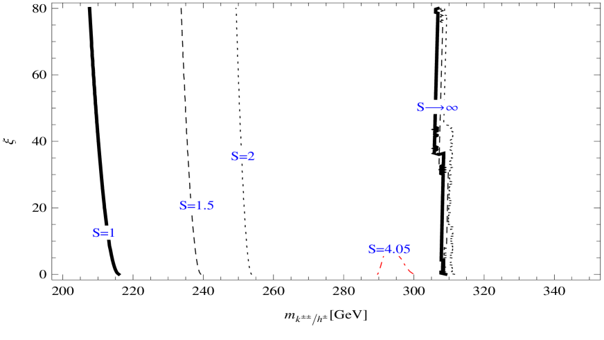
Figure 2: The strength of EWPT with $\lambda=0.1297$ and $\mu^{2}\sim\lambda v^{2}_{0}$

In fact, the mass of Goldstone boson is much smaller than that of the $W^{\pm}$ boson or the $Z$ boson so the contribution of Goldstone boson must be very small in the effective potential. Hence, the lines in Fig.2 are almost vertical or almost parallel to the axis $\xi$. These results match those of Ref.Arefe . This shows that the strength of EWPT is gauge independent.

In addition, the new particles have large masses, so they provide valuable contributions to the EWPT in the Landau gauge or in an arbitrary gauge. The charge of these particles increases their contributions. In particular, $k^{\pm\pm}$ is the doubly charged scalar, so its coefficients in the effective potential are also greater than two times the coefficient of $W^{\pm}$ boson (because of the fact that the doubly charged particle ($k^{\pm\pm}$) always appears in pairs with the singly charged one ($h^{\pm}$), and by our approximation, with the same masses: $m_{k^{\pm\pm}}=m_{h^{\pm}}$).

Furthermore, we find that models having doubly charged particles, provide a very strong first-order EWPT, such as the Georgi–Machacek model chiang3 and they are being tested by LHC chiang1 ; chiang2 .

According to Nielsen’s identity, in $\hbar$ expansion, the one-loop effective potential is gauge independent at each order by $\hbar$ 1101.4665 , but the general potential still is gauge dependent. However this dependence is not important as in our above analysis.

IV Constraints on coupling constants in the Higgs potential

In order to have the first order phase transition, the masses of the new charged scalars $m_{h^{\pm}}$ and $m_{k^{\pm\pm}}$ must be smaller than $350$ GeV. Therefore, we obtain

$$p^{2}v^{2}_{0}<(300\text{ GeV})^{2},$$ (22)

and

$$q^{2}v^{2}_{0}<(300\text{ GeV})^{2}\,.$$ (23)

From the above equations, we obtain the following limits: $0<p<1.22$ and $0<q<1.22$. However, to find these accurate values of $m_{h^{\pm}}$ and $m_{k^{\pm\pm}}$, other considerations are also needed.

In the ZB model, the tiny masses of neutrino are generated at two loops, so $m_{h^{\pm}}$ and $m_{k^{\pm\pm}}$ cannot be very heavy test1 . From the experimental point of view, it is interesting to consider new scalars light enough to be produced at the LHC. The theoretical arguments lead to the fact that the scalar masses should be a few TeVs, to avoid unnaturally large one-loop corrections to the Higgs boson mass which would cause a hierarchy problem. Therefore, these upper bounds of new scalar masses can be 2 TeVs test . Contacting to neutrino oscillation data, in the decay $k^{\pm\pm}\longrightarrow ll$, the branching ratio to $\tau\tau$ is very small in the ZB model, less than about $1\%$. Then, a conservative limit is $m_{k{\pm\pm}}>200$ GeV. In the ZB model, we can have the decay $k^{\pm\pm}\longrightarrow h^{\pm}h^{\pm}$, so $2m_{h^{\pm}}<m_{k^{\pm\pm}}$. Therefore, our results in Eqs. (22) and (23) are consistent with the above estimation.

Recently, the experimental groups at LHC (ATLAS and CMS Collaborations) atlas have reported an experimental anomaly in diboson production with apparent excess in boosted jets of the $W^{+}W^{-},W^{\pm}Z$ and $ZZ$ channels at around 2 TeV invariant mass of the boson pair.

In addition, the calculation the Higgs coupling to photons (due to charged particles in the loop diagram) can be related to neutrino mass and $CP$ violation which are the key of matter and antimatter asymmetry. This study will be investigated in a future publication.

V CONCLUSION AND OUTLOOKS

In this paper we have investigated the EWPT in the ZB model using the high-temperature effective potential. The EWPT is strengthened by the new scalars to be the strongly first-order, the phase transition strength ranges from 1 to 4.15. The new charged scalars $h^{\pm}$ and $k^{\pm\pm}$ are triggers for the first-order EWPT. Our results may be better than the results in Ref. pelto .

It is known that if a particle has the bigger charge, the decay rate will be larger. In their decay or scattering channels, we can estimate their mass, or the parameter domain in the Higgs potential. So the charge of particle also affects the parameter domain in the Higgs potential or signatures of the charge of new particles ($h^{\pm},k^{\pm\pm}$) are hidden in the parameter domain, which in turn can indirectly affect the EWPT. However, in our calculation process, we looked for the mass domain of the new particles to have a first-order phase transition. Then we will extract the parameter domain in the Higgs potential. If they match with values derived from scattering channels, our solution will be viable. Therefore, signatures of the charge may be an external condition for checking or limiting the parameter domain in our solution.

In addition, the EWPT can be calculated in a different way as in Ref.1101.4665 ; Arefe . In order to determine $T_{N}$ or $T_{E}$, we will examine this problem in conjunction with the $CP$-violation.

In the ZB model, the tiny mass of neutrino which can be explained at two loop level induced by couplings between charged Higgs boson and neutrino; and this can be a reason of the matter-antimatter asymmetry and $CP$-violation. The behavior of charged Higgs boson is also very interesting. Therefore, in the next works, we can investigate the ratio $m^{\prime}_{h^{\pm}/k^{\pm\pm}}$ by using neutrino data and the sphaleron rate. We will investigate the $CP$- violation and beyond issues of the baryon asymmetry problem through neutrino physics.

Furthermore, the sphaleron is an important process in baryogenesis and leptogenesis so we will continue to calculate and test the sphaleron solution in this model with the COSMOTRANSITION code cosmotran . This code used a Bessel function for $v(r)$ but it is not flexible in changing the value of the wall.

With this region of self couplings in the Higgs potential, we can serve as basis for the calculation of other effects connected to data of the LHC, such as diphoton decay of Higgs boson, etc.

References

- (1) A. D. Sakharov, JETP Lett.5, 24 (1967).
- (2) V. Mukhanov, Physical Foundations of Cosmology (Cambridge University Press, Cambridge, England, 2005), M. l Dine, R. G. Leigh, P. Huet, A. Linde, and D. Linde, Phys. Rev. D 46, 550 (1992).
- (3) A. G. Cohen, D. B. Kaplan, and A.E. Nelson, Ann. Rev. Nucl. Part. Sci. 43, 27 (1993); A. G. Cohen, in Physics at the Frontiers of the Standard Model, 2nd Rencontres du Vietnam (Editions Frontiers, Ho Chi Minh City, 1995), pp. 311.
- (4) K. Kajantie, M. Laine, K. Rummukainen, and M. Shaposhnikov, Phys. Rev. Lett. 77, 2887 (1996); F. Csikor, Z. Fodor, and J. Heitger, Phys. Rev. Lett. 82, 21 (1999); J. Grant, M. Hindmarsh, Phys. Rev. D 64, 016002 (2001); M. D’Onofrio, K. Rummukainen, A. Tranberg, JHEP 08, 123 (2012).
- (5) M. D’Onofrio, K. Rummukainen, A. Tranberg, Phys. Rev. Lett. 113, 141602 (2014).
- (6) M. Bastero-Gil, C. Hugonie, S. F. King, D. P. Roy, and S. Vempati, Phys. Lett. B 489, 359 (2000); A. Menon, D. E. Morrissey, and C. E. M. Wagner, Phys. Rev. D 70, 035005 (2004); S. W. Ham, S. K. Oh, C. M. Kim, E. J. Yoo, and D. Son, Phys. Rev. D 70, 075001 (2004).
- (7) J. M. Cline, G. Laporte, H. Yamashita, S. Kraml, JHEP 0907, 040 (2009).
- (8) S. Kanemura, Y. Okada, E. Senaha, Phys. Lett. B 606, 361-366 (2005); G. C. Dorsch, S. J. Huber, J. M. No, JHEP 10 (2013) 029.
- (9) S. W. Ham, S-A Shim, and S. K. Oh, Phys. Rev. D 81, 055015 (2010).
- (10) S. Das, P. J. Fox, A. Kumar, and N. Weiner, JHEP 1011, 108 (2010); D. Chung and A. J. Long, Phys. Rev. D 84, 103513 (2011); M. Carena, N. R. Shaha, and C. E. M. Wagner, Phys. Rev. D 85, 036003 (2012); A. Ahriche and S. Nasri, Phys. Rev. D 85, 093007 (2012); D. Borah and J. M. Cline, Phys. Rev. D 86, 055001 (2013).
- (11) V. Q. Phong, V. T. Van, and H. N. Long, Phys. Rev. D 88, 096009 (2013), arXiv:1309.0355; V. Q. Phong, H. N. Long, V. T. Van, N. C. Thanh, Phys. Rev. D 90, 085019 (2014), arXiv:1408.5657(hep-ph); V. Q. Phong, H. N. Long, V. T. Van, L. H. Minh, Eur. Phys. J. C 75,342 (2015), arXiv:1409.0750(hep-ph); J. Sá Borges, R. O.Ramos, Eur. Phys. J. C 76: 344 (2016).
- (12) J. R. Espinosa, T. Konstandin and F. Riva, Nucl. Phys. B 854, 592 (2012).
- (13) S. Kanemura, E. Senaha, T. Shindou and T. Yamada, JHEP 1305, 066 (2013).
- (14) D. J. H. Chung and A. J. Long, Phys. Rev. D 81, 123531 (2010) .
- (15) G. Barenboim and N. Rius, Phys. Rev. D 58, 065010 (1998).
- (16) S. Profumo, M. J. Ramsey-Musolf, G. Shaughnessy, JHEP 0708 (2007) 010; S. Profumo, M. J. Ramsey-Musolf, C. L. Wainwright, P. Winslow, Phys. Rev. D 91, 035018 (2015); D. Curtin, P. Meade, C-T. Yu, JHEP 11(2014)127; M. Jiang, L. Bian, W. Huang, J. Shu, Phys. Rev. D 93, 065032 (2016).
- (17) M. Carena, G. Nardini, M. Quiros, C. E.M. Wagner, Nucl. Phys. B 812:243-263 (2009); A. Katz, M. Perelstein, M. J. Ramsey-Musolf, P. Winslow, Phys. Rev. D 92, 095019 (2015); J. Kozaczuk, S. Profumo, L. S. Haskins, C. L. Wainwright, JHEP 1501 (2015) 144.
- (18) H. H. Patel, M. J. Ramsey-Musolf, Phys.Rev. D. 88, 035013 (2012); N. Blinov, J. Kozaczuk, D. E. Morrissey, C. Tamarit, Phys. Rev. D 92, 035012 (2015); S. Inoue, G. Ovanesyan, M. J. Ramsey-Musolf, Phys. Rev. D 93, 015013 (2016).
- (19) H. H. Patel, M. J. Ramsey-Musolf, JHEP 1107 (2011) 029; G. W. Anderson and L. J. Hall, Phys. Rev. D 45, 2685 (1992); H. H.Patel and M.J.Ramsey-Musolf, M. Garny and T.Konstandin, JHEP 1207, 189 (2012); C.W. Chiang, M.J.Ramsey-Musolf and E. Senaha, Phys. Rev. D 97, 015005 (2018), arXiv:1707.09960 [hep-ph].
- (20) C. W. Chiang, T. Yamada, Phys. Let. B 06, 048 (2014).
- (21) J. R. Espinosa, T. Konstandin, J. M. No and M. Quiros, Phys. Rev. D 78, 123528 (2008).
- (22) A. Zee, Nucl. Phys. B 264, 99 (1986); K. S. Babu, Phys. Lett. B 203, 132 (1988).
- (23) H. Okada, T. Toma, K. Yagyu, Phys. Rev. D 90, 095005 (2014); S. Baek, JHEP 08, 023 (2015); H. Hatanaka, K. Nishiwaki, H. Okada, Y. Orikasa, Nucl. Phys. B 894 (2015).
- (24) G. W. Anderson and L. J. Hall, Phys. Rev. D 45, 2685 (1992).
- (25) C. W. Chiang, A. L. Kuo, Toshifumi Yamada, JHEP 01, 120 (2016).
- (26) C. W. Chiang, A. L. Kuo, Toshifumi Yamada, Phys. Rev. D 85, 095023 (2012).
- (27) J. Herrero-Garcia, M. Nebot, N. Rius, A. Santamaria, Nucl. Part. Phys. Proc. 273, 1678 (2016).
- (28) J. Herrero-Garcia, M. Nebot, N. Rius and A. Santamaria, Nucl. Phys. B 885, 542 (2014).
- (29) G. Aad et al, [ATLAS Collaboration], JHEP 12 (2015) 55, arXiv:1506.00962 [hep-ex]; V. Khachatryan et al [CMS Collaboration], JHEP 1408 (2014) 173, arXiv:1405.1994 [hep-ex].
- (30) J. T. Peltoniemi, J. W. F. Valle, Phys. Lett. B 304, 147 (1993).
- (31) C. L. Wainwright, Comput. Phys. Commun. 183, 2006 (2012).