Spectral-Line Survey at Millimeter and Submillimeter Wavelengths
toward an Outflow-Shocked Region, OMC 2-FIR 4

Abstract

We performed the first spectral-line survey at 82–106 GHz and 335–355 GHz toward the outflow-shocked region, OMC 2-FIR 4, the outflow driving source, FIR 3, and the northern outflow lobe, FIR 3N. We detected 120 lines of 20 molecular species. The line profiles are found to be classifiable into two types: one is a single Gaussian component with a narrow ($<$ 3 km s^-1) width and another is two Gaussian components with narrow and wide ($>$ 3km s^-1) widths. The narrow components for the most of the lines are detected at all positions, suggesting that they trace the ambient dense gas. For CO, CS, HCN, and HCO⁺ , the wide components are detected at all positions, suggesting the outflow origin. The wide components of C³⁴S, SO, SiO, H¹³CN, HC¹⁵N, H${}_{2}^{13}$CO, H₂CS, HC₃N, and CH₃OH are detected only at FIR 4, suggesting the outflow-shocked gas origin. The rotation diagram analysis revealed that the narrow components of C₂H and H¹³CO⁺ show low temperatures of 12.5$\pm$1.4 K, while the wide components show high temperatures of 20–70 K. This supports our interpretation that the wide components trace the outflow and/or outflow-shocked gas. We compared observed molecular abundances relative to H¹³CO⁺ with those of the outflow-shocked region, L1157 B1, and the hot corino, IRAS 16293-2422. Although we cannot exclude a possibility that the chemical enrichment in FIR 4 is caused by the hot core chemistry, the chemical compositions in FIR 4 are more similar to those in L1157 B1 than those in IRAS 16293-2422.

1 Introduction

Enormous progress has been achieved in the past few decades in studying the chemical composition of dense molecular gas in star-forming regions. The chemical composition and evolution in the dense interstellar medium (ISM) themselves are of great interest. In addition, they are very useful for diagnostics of protostar or protoplanetary disk evolution, and also of shocks and energy sources of extragalactic nuclei. Shock chemistry is a key to understand the chemical composition of ISM, because shock waves are ubiquitous in astrophysical phenomena; evidence for shock is usually found in outflows and jets associated with star formation. One of the best-studied shocked regions is L 1157 B1. Recently, spectral line surveys were performed at the wavelengths of 3 mm and 500 $\mu$m, which revealed the chemical composition of the outflow-shocked region (Codella et al., 2001; Sugimura et al., 2011; Yamaguchi et al., 2012; Benedettini et al., 2012). However, observational studies of shocked regions focused on molecular compositions have been limited to a few sources, although theoretical studies on shock physics have been extensively made since the 1980s (McKee & Hollenbach, 1980; Neufeld et al., 1995). Physical and chemical properties of shocked gas depend on physical conditions of ambient medium and shock velocity. To unveil the nature of the shocked gas, we need to observe various outflow-shocked regions.

FIR 4 is located in OMC2, which is the northern part of the Orion A Molecular cloud ($d$ = 400 pc, Menten et al., 2007; Sandstrom et al., 2007; Hirota et al., 2008). This region is known as an active cluster-forming region where three 3.6-cm free-free emission sources and nine MIR sources are embedded(Reipurth et al., 1999; Nielbock et al., 2003). Williams et al. (2003) and Takahashi et al. (2008) found a molecular outflow driven by FIR 3 in the ¹²CO (1–0, 3–2) lines. Shimajiri et al. (2008) suggested that the outflow driven by FIR 3 interacts with the 0.07 pc-scale dense gas associated with FIR 4 (FIR 4 clump), from morphological, kinematical, chemical, and physical evidence. Morphologically, the length ($\sim$0.2 pc) of the northeast (NE) CO (1–0, 3–2) outflow lobe from FIR 3 is smaller than that of the southwest (SW) lobe ($\sim$0.1 pc). Moreover, the FIR 4 clump is located at the tip of the SW lobe. These features strongly suggest that the SW lobe has been stemmed by the FIR 4 clump. In addition, the shock tracers of SiO ($v$=0, 2–1) and CH₃OH ($J_{K}$=7_K–6_K ; $K$=-1, 0, 2) are detected at the interface between the SW lobe and the FIR 4 clump. Moreover, the abrupt increase of the velocity width of CO, H¹³CO⁺, CH₃OH, and SiO at the interface between the SW lobe and the FIR 4 clump suggests the presence of the outflow interaction. Consequently, it is likely that the high-velocity outflow collides with the quiescent dense clump. Hence, FIR 4 is a good target to investigate the chemistry of the outflow-shocked region.

This paper is organized as follows: In Sect. 2, we describe our targets, FIR 3N, FIR 3, and FIR 4. In Sect. 3, we describe the Nobeyama 45 m and Atacama submillimeter telescope experiment (ASTE) observations and data reduction procedures using the common astronomy software application (CASA). In Sect. 4, we present results of our line survey observations in the 82–106 GHz and 335–355 GHz toward FIR 3N, FIR 3, and FIR 4. In Sect. 5, we discuss the nature of the dense gas in FIR 4 on the basis of the velocity widths, rotation temperatures, and fractional abundances of the detected molecules. We compare rotation temperatures and column densities among molecules detected in the Nobeyama 45 m and ASTE spectral line surveys. At the end of this section, we show the fractional abundances relative to H¹³CO⁺ in FIR 4. Then, we compare them with the corresponding abundances in the L 1157 B1 and IRAS 16293-2422 regions. In Sect. 6, we summarize this paper.

2 Our Targets

Our target sources are FIR 3N, FIR 3, and FIR 4 in OMC 2, as indicated in Fig. 1. Table 1 shows the positions of the three sources, the CO (1–0) intensities, and the dust continuum flux densities at 1.1 mm with the AzTEC (Shimajiri et al., 2011, also see Sect. 4.5). Here, we describe the detailed features of the sources.

2.1 FIR 3N

FIR 3N is a CO peak position in the northeastern lobe of the blue-shifted outflow driven by FIR 3 (Takahashi et al., 2008). In this area, it is likely that no prominent shock occurs for the following reasons. No dense condensations have been found by the H¹³CO⁺ (1–0), N₂H⁺ (1–0), and 1.1 mm dust continuum observations (Ikeda et al., 2007; Tatematsu et al., 2008; Shimajiri et al., 2015). Although Yu et al. (1997) and Stanke et al. (2002) found several H₂ knots, the shock tracers such as the SiO ($v$=0, 2–1) and CH₃OH ($J_{K}$=7_K–6_K;$K$=-1,0,1) lines have not been detected toward the outflow lobe (Shimajiri et al., 2008).

2.2 FIR 3

FIR 3 is known as a Class 0/I object, which ejects the molecular outflow along the northeast-southwest direction with a dynamical time scale of 1.4 $\times$ 10⁴ yr (Chini et al., 1997; Takahashi et al., 2008). The momentum flux, $F_{\rm CO}$, of the northeastern blue-shifted lobe is 2.3 $\times$10^-3 $M_{\odot}$ km s^-1 yr^-1, the highest value in the OMC 2/3 region. The 1.3 mm and 850 $\mu$m dust continuum emission and two MIR sources (MIR 21 and 22) are associated with the source FIR 3 (Chini et al., 1997; Johnstone & Bally, 1999; Nielbock et al., 2003). FIR 3 has been identified as SOF 2N in the 4.5 $\mu$m and 37.1 $\mu$m emission by the SOFIA/FORCAST and its total luminosity is estimated to be 300 $L_{\odot}$ (Adams et al., 2012).

2.3 FIR 4

FIR 4 is the strongest dust-continuum source in the OMC 2 region (Chini et al., 1997; Shimajiri et al., 2015). The Nobeyama Millimeter Array (NMA) observations at an angular resolution of $\sim$3$\arcsec$ have revealed that FIR 4 consists of eleven compact dust clumps (Shimajiri et al., 2008). The source has been identified as SOF 3 in the 4.5 $\mu$m and 37.1 $\mu$m emission by the SOFIA/FORCAST, and its total luminosity is estimated to be 50 $L_{\odot}$. However, the clumps detected in the 3.3 mm dust continuum emission by Shimajiri et al. (2008) do not coincide with the 8–160 $\mu$m emission sources (Adams et al., 2012). Shimajiri et al. (2008) concluded that the molecular outflow driven from FIR 3 interacts with the dense gas associated with FIR 4 (see Sect. 1). Thus, FIR 4 is a good target to investigate the chemistry of an outflow-shocked region.

3 Observations and Data Reduction

3.1 Nobeyama 45m Observations

The Nobeyama 45 m observations were conducted in 2011 January toward the FIR 4 region in addition to the driving source of the molecular outflow, FIR 3, and the northeast outflow lobe, FIR 3N, as shown in Fig. 1. In Table 1, the positions of FIR 4, FIR 3, and FIR 3N, are summarized. The position of FIR 3N corresponds to the CO peak position of the northeast lobe. Around FIR 3N, there is no sign of the interaction between the outflow and the ambient quiescent gas (Shimajiri et al., 2008). The position of FIR 4 corresponds to the CO peak position of the southeast lobe.

The data were taken in the position-switching mode. The T100 receiver, which is a dual polarization sideband-separating SIS receiver, was used in combination with the Fast Fourier Transform Spectrometer (SAM45) providing a total bandwidth of 16 GHz (=((4 GHz for LSB) + (4 GHz for USB)) $\times$ 2 polarization) and a frequency resolution of 488.24 kHz, corresponding to $\sim$1.5 km s^-1 at 100 GHz (Nakajima et al., 2008). To cover the frequency range between 82 and 106 GHz, we used three different frequency settings (82–86 & 94–98 GHz, 86–90 & 98–102 GHz, and 90-94 & 102–106 GHz). Pointing was checked by observing the Ori-KL SiO maser emission every hour, and was shown to be accurate within a few arc-seconds. The parameters for the observations are summarized in Table 2. The main-beam efficiency was 40%. The system noise temperature was around 150 K, resulting in the rms noise level of 10–40 mK in $T_{\rm A}^{*}$, as summarized in Table 3.

3.2 ASTE Observations

The ASTE observations at 335–355 GHz were conducted toward the same sources of FIR 4, FIR 3, and FIR 3N. The data were taken in 2012 December in the position-switching mode. The CATS345 receiver, which is a side-band separating (2SB) mixer receiver, was used in combination with the MAC correlator providing a bandwidth of 512 MHz in each of 4 arrays and a frequency resolution of 0.5 MHz, corresponding to $\sim$0.5 km s^-1 at 345 GHz (Sorai et al., 2000; Inoue et al., 2008). The adjust frequency coverage overlaps by 112 MHz. Thus, one frequency setting can cover the frequency range of $\sim$1.6 GHz. We used 13 different frequency settings to cover the frequency range of 20 GHz ($\sim$1.6 GHz $\times$ 13 arrays). The main-beam efficiency of the telescope was $\sim$50%. The system noise temperature was 200–500 K, and the rms noise level was 18–42 mK in $T_{\rm A}^{*}$, as summarized in Table 3. Pointing of the telescope was checked by observing the CO (3–2) line emission from O-Cet every two hours, and was shown to be accurate within 2$\arcsec$. The observational parameters are summarized in Table 2.

3.3 Data Reduction

We used the 3.2.1 version of the Common Astronomy Software Application (CASA) package (McMullin et al., 2007) to reduce the data obtained with the Nobeyama 45 m and ASTE telescopes. The CASA package is developed for the Atacama Large Millimeter/submillimeter Array (ALMA), and is also available for reducing data obtained by a single-dish telescope such as the Nobeyama 45 m telescope and the ASTE telescope. Here, we describe detailed steps of the data reduction process. In the first step, edge channels of each correlator band were flagged out using the task $sdflag$, since the sensitivity of the edge channels drops. The SAM45 spectrometer of the Nobeyama 45 m telescope provides 4096 frequency channels, so that the data for the channel numbers from 1 to 300 and from 3796 to 4096 were flagged out. The data of the MAC spectrometer of the ASTE telescope provides 1024 frequency channels. Hence, the data for the channel numbers from 1 to 100 and from 924 to 1024 were flagged out. In the second step, we determined the baseline of each spectrum using the task $sdbaseline$. The ”auto” baseline mode automatically detects line emission regions and decides the baseline from the emission-free regions. We adopted a signal-to-noise ratio (S/N) of 5 as the threshold level for detecting the signal regions. In the third step, we used the task $sdaverage$ to average all the spectra in one observing sequence at each observed position with a weight of 1/$T_{\rm sys}^{2}$, where $T_{\rm sys}$ denotes the system noise temperature. In the fourth step, we used the task $sdflag$ again to flag out bad channels in the averaged spectra. In the fifth step, we merged all the averaged spectra into one file using the task $sdcoadd$. In the final step, we averaged all the averaged spectra with a weight of 1/$T_{\rm sys}^{2}$ using the task $sdaverage$.

4 Results and Analysis of Molecular Lines

4.1 Spectrum and Line Identification

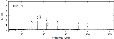
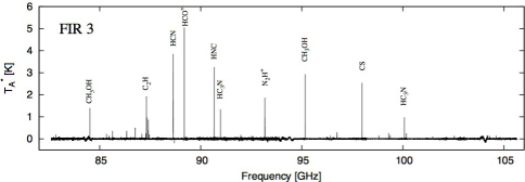
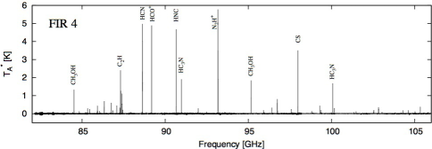
Figure 2: Compressed spectra of FIR 3N, FIR 3, and FIR 4 observed in 82–106 GHz.

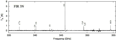
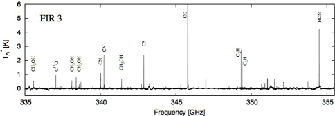
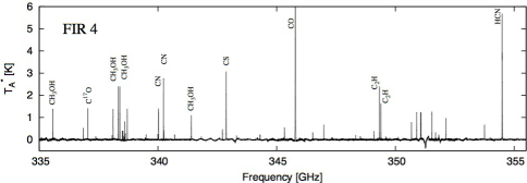
Figure 3: Compressed spectra of FIR 3N, FIR 3, and FIR 4 observed in 335–355 GHz.

Figures 2 and 3 show the compressed spectra from 82 to 106 GHz and from 335 to 355 GHz, respectively. The rms noise ranges from 10 mK to 41 mK and from 19 mK to 43 mK in $T_{\rm A}^{*}$, respectively. We adopted a criterion that a signal-to-noise ratio should be higher than 3 with the spectral line catalog by Lovas et al. (2004) to identify molecular lines in our detected spectra.

As a result, our 3-mm and 850-$\mu$m line surveys have identified 120 lines of 20 molecular species including CH₃CCH, CH₃CHO, and C₃H₂ as well as S-bearing molecules such as H₂CS, SO, and HCS⁺. In addition, 40 lines and 12 rare isotopic species (¹³C, ¹⁵N, ¹⁷O, ¹⁸O, ³⁴S, and D) have been detected. See Appendix for the descriptions of the detected species and their line profiles. The numbers of the detected lines and species at each position are listed in Table 4 and the detected molecules are summarized in Table 5.

4.2 Line Parameters with Narrow and Wide Velocity Components

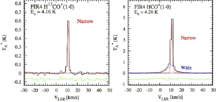
Figure 4: Two representative examples of the Gaussian fitting. Left: one narrow component (red line) can be well fitted to the H¹³CO⁺ (1–0) line profile (black lines) at FIR 4. The green lines show the residual spectrum. Right: both narrow (red) and wide (blue) components are required for the HCO⁺ (1–0) line.

We found that all the identified molecular lines can be classified into the following two types according to their line profiles. One is a single narrow line whose velocity width is 3 km s^-1 or less, and the other is a line accompanying a wide component with the line width of 3 km s^-1 or larger in addition to the narrow component. Figure 4 shows two representative spectra of the H¹³CO⁺ (1–0) and HCO⁺ (1–0) emission at FIR 4. The H¹³CO⁺ (1–0) line profile can well be fitted by a single Gaussian component with a narrow velocity width (1.85 km s^-1), while the HCO⁺ (1–0) line profile consists of narrow (1.85 km s^-1) and wide (8.12 km s^-1) components. We performed the Gaussian fitting for all the lines by the following steps. First, we applied one Gaussian component with a narrow width to the observed spectrum. When the signal-to-noise ratio (S/N) of the peak residual intensity is less than 2, we regard the spectral line as a single narrow line. If not, we applied two Gaussian components to the observed spectrum. Hereafter, we simply refer to the Gaussian component with the narrow velocity width as $Narrow$, and the Gaussian component with the wide velocity width as $Wide$. In the Gaussian fitting, we also obtained the line parameters such as peak intensity, systemic velocity, and velocity width, as shown in Tables A2–A4. In this survey, the lines with hyperfine structure (HFS) such as the HCN, H¹³CN, N₂H⁺, and NH₂D lines are detected. For the N₂H⁺ and NH₂D spectra having only the narrow components, we also applied the HFS fitting (See Sect. A.1). We assumed that all the HFS components of each line have the same LSR velocity and the same velocity width. We used the frequency differences among the HFS components listed in the spectral line catalog by Lovas et al. (2004). The obtained line parameters of $V_{\rm sys}$ and d$V_{\rm FWHM}$ are comparable to those obtained by the Gaussian fitting. However, the intensities obtained by the HFS fitting are different from those obtained by the Gaussian fitting, suggesting that the results of the Gaussian fitting are affected by the blending of the HFS components.

4.2.1 Spectra Having One Narrow Component

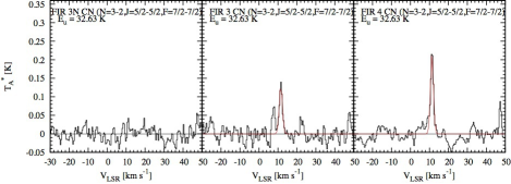
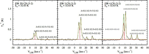
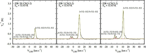
Figure A1: CN spectra with the upper energy levels in K. The best-fit narrow component of each transition is shown by the red line, and the green line shows the sum of all the components.

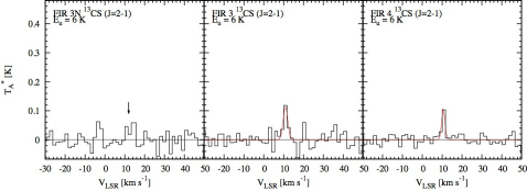
Figure A10: ¹³CS spectra. The vertical arrow in the right panel shows the emission-like feature.

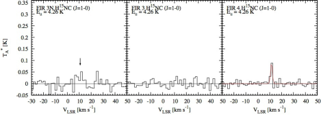
Figure A18: H¹⁵NC spectra. The vertical arrow in the left panel shows the detection, but the peak is not fitted well by the single Gaussian component due to insufficient velocity resolution.

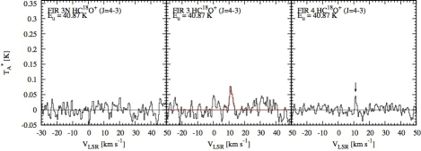
Figure A19: HC¹⁸O⁺ spectra. The vertical arrow in the right panel shows the emission-like feature.

The CN, C¹⁷O, C₂H, HNC, HN¹³C, H¹³CO⁺, N₂H⁺, c-C₃H₂, and CH₃CN lines are found to have one narrow component and are detected at the three positions (see Table 5 and Figs. A1–A9). The velocity widths of the lines range from 0.6 to 4.8 km s^-1 (mean: 2.1$\pm$0.7 km s^-1). Only one channel in the c-C₃H₂ and CH₃CN spectra at FIR 3N has emission more than 3$\sigma$ due to poor velocity resolution. Thus, the fitting points (velocity channels) are not sufficient to make a reasonable fit by the single Gaussian component. Since these spectra at FIR 4 have only narrow components, these spectra at FIR 3N are also likely to have only narrow components. The ¹³CS, HDCO, HNCO, CH₃CCH, and CH₃CHO lines also have one narrow component with velocity widths from 1.3 to 3.8 km s^-1 (mean: 2.6$\pm$0.7 km s^-1), although they are not detected at FIR 3N (see Table 5 and Figs. A10–A14). The HCS⁺, NH₂D, and H₂CO lines have one narrow component and detected only at FIR 4 (see Table 5 and Figs. A15–A17). The velocity widths of the lines range from 1.5 to 3.8 km s^-1 (mean: 2.1$\pm$1.0 km s^-1). The H¹⁵NC line is detected at FIR 3N and FIR 4 and has one narrow component. The velocity width at FIR 4 is 1.82 km s^-1 (see Table 5 and Fig. A18). The spectrum of H¹⁵NC at FIR 3N is not fitted well by the single Gaussian component due to insufficient resolution. Since the H¹⁵NC spectrum at FIR 4 has an only narrow component, the H¹⁵NC one at FIR 3N is also likely to have an only narrow component. The HC¹⁸O⁺ line is detected only at FIR 3 and has one narrow component with a velocity width of 2.2 km s^-1 (see Table 5 and Fig. A19).

4.2.2 Spectra Having Narrow and Wide Components

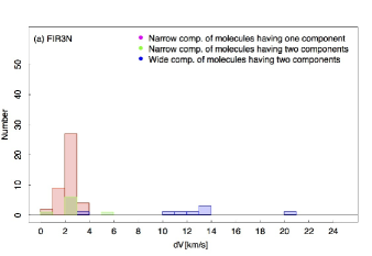
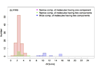
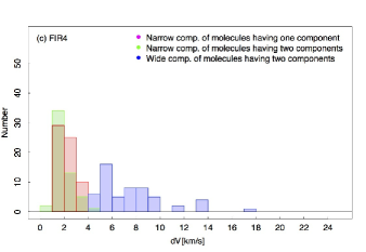
Figure 5: Histograms of the velocity widths in FWHM for the detected lines toward (a) FIR 3N, (b) FIR 3, and (c) FIR 4. The red histograms correspond to the narrow components of the molecules having an only one component, which are determined by Gaussian fitting, as shown in Fig. 4. The green and blue histograms correspond to the narrow and wide components of the molecules having two components.

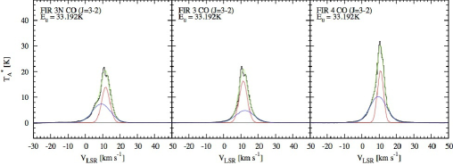
Figure A20: CO spectra. The best-fit narrow and wide components are shown by the red and blue lines, respectively, and the green line shows the sum of the two components.

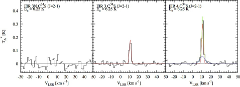
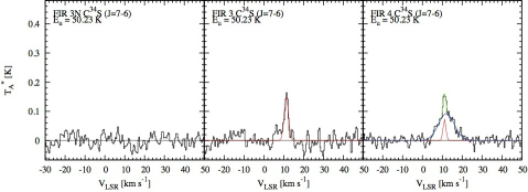
Figure A24: C³⁴S spectra

The CO, CS, HCN, and HCO⁺ lines are found to have narrow and wide components, and they are detected at the three positions (see Table 5 and Figs. A20–A23). The narrow and wide velocity widths of the lines range from 0.9 to 5.6 km s^-1 (mean: 2.9$\pm$1.0 km s^-1) and from 3.3 to 20.2 km s^-1 (mean: 11.7$\pm$3.5 km s^-1), respectively. The C³⁴S, SO, SiO, H¹³CN, HC¹⁵N, H${}_{2}^{13}$CO, H₂CS, HC₃N, and CH₃OH lines also have narrow and wide components, but the wide components are detected only at FIR 4 (see Table 5 and Figs. A24–A32). The ranges of the narrow and wide velocity widths are 0.6–3.3 km s^-1 (mean: 1.9$\pm$0.7 km s^-1) and 4.2–17.3 km s^-1 (mean: 7.1$\pm$2.5 km s^-1), respectively. Figure 5 shows histograms of the velocity widths of the fitted Gaussian components for the detected lines.

4.3 Optical Depth

Since the same rotational transitions of the normal species and their rare isotropic species are detected for HCO⁺, CS, HCN, and HNC, we estimated optical depths of the transitions. Assuming the same excitation temperature for the two isotopic species and the isotopic ratios, $R_{\rm i}$, of 22 for ³²S/³⁴S and 62 for ¹²C/¹³C (Langer & Penzias, 1993), we evaluated the optical depth of the normal species line by the following equation:

$$\frac{T_{A}^{*}({\rm i)}}{T_{A}^{*}({\rm n})}=\frac{1-e^{-\tau(\rm{n)/R_{\rm i}}}}{1-e^{-\tau(\rm{n})}}.$$ (1)

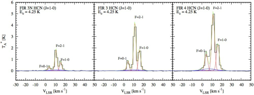
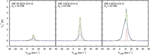
Figure A22: HCN spectra

Here, $T_{\rm A}^{*}({\rm n}$) and $\tau(\rm{n})$ are the observed antenna temperature and the optical depth of the normal species, whereas $T_{\rm A}^{*}({\rm i}$) is the observed antenna temperature of the rare isotopic species. As a result, the normal species lines of the above molecules are found to be optically thick, as shown in Table 6. In particular, the optical depth of the wide component of the HCN (1–0) line exceeds 10. The large optical depth might be, however, artificial, because we assumed the same intensity ratios of the narrow to wide components for the hyperfine structure of HCN; The wide components of the HFS lines heavily overlap with one another, and cannot be well separated (see Fig. A22 and A27 and Appendix A.2.6).

4.4 Rotation Diagram

To estimate the rotation temperature and column density of the detected molecules, we made rotation diagrams by using the data taken with the Nobeyama 45 m and ASTE telescopes. This method is based on the relationship among the beam-averaged column density, $N_{\rm mol}$, the rotation temperature, $T_{\rm rot}$, and the line intensity, $\int$($T_{\rm R}^{*}$)$dv$, under the assumption of the LTE and optically thin conditions (Turner, 1991):

$$\ln L=\ln(\frac{N_{\rm mol}}{Q(T_{\rm rot})})-\frac{E_{\rm u}}{k}\frac{1}{T_{\rm rot}},$$ (2)

and

$$L=\frac{3k\int T_{\rm R}^{*}dv}{8\pi^{3}\nu S\mu^{2}g_{I}g_{K}}.$$ (3)

Here, $E_{\rm u}$, $S$, and $\mu$ are the upper state energy, the intrinsic line strength and the relevant dipole moment. The values of $E_{\rm u}$ and $S\mu^{2}$ are obtained from Splatalogue, except for CH₃CN and CH₃CCH. For CH₃CN and CH₃CCH, these values are from the Cologne Database for Molecular Spectroscopy (CDMS). The factors of $g_{\rm I}$ and $g_{\rm K}$ are the reduced nuclear spin degeneracy and the $K$-level degeneracy, respectively. For linear molecules, $g_{\rm I}$=$g_{\rm K}$=1 for all energy levels. We used the partition functions, $Q(T_{\rm rot})$=$\sum_{i=1}g_{i}{\rm exp}(-E_{i}/kT_{\rm rot})$, where $g_{i}$ and $E_{i}$ are the degeneracy and energy of the $i$-th state. Rotational energies of each molecule are taken from CDMS.

For the line intensity, we adopted $T_{\rm R}^{*}$=$T_{\rm A}^{*}$/$\eta_{\rm MB}$/$f$, where $\eta_{\rm MB}$ and $f$ are the main-beam efficiency of the telescope and the beam filling factor of the source, respectively. The factor $f$ is given by $f=\theta_{\rm s}^{2}/(\theta_{\rm s}^{2}+\theta_{\rm b}^{2}$), where $\theta_{\rm s}$ and $\theta_{\rm b}$ are the source size and the telescope beam size, respectively (Kim et al., 2000). Here, we assumed that $\theta_{\rm s}$ is 17$\arcsec$ for FIR 3 and 19$\arcsec$ for FIR 4 which are the sizes of the dust condensations of FIR 3 and FIR 4 measured in the 1.1 mm dust continuum emission (Chini et al., 1997). For FIR 3N, we assumed $f$=1 since the emission at FIR 3N seems to trace the extended structures of the outflow and ambient gas (see Sect. 5.1). Finally, we obtained the integrated intensity of each line by $\frac{1.06\times T_{\rm A}^{*}\times dV}{f\eta_{\rm MB}}$, where a correction factor of 1.06 is applied for the Gaussian profile and $dV$ is the FWHM of the velocity profile. According to Eq. (2), $N_{\rm mol}$ and $T_{\rm rot}$ can be determined by a best-fit straight line in a plot of log $L$ as a function of $E_{\rm u}/k$. As a result, we obtained the rotation temperatures and the column densities for 12 molecules, as shown in Table 8. The rotation diagrams of individual molecules are shown in Figs. A33 to A44.

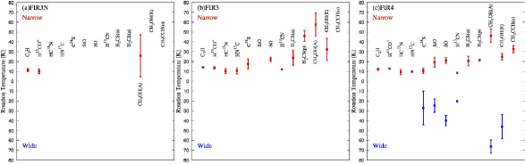
Figure 6: Comparison of the rotation temperatures between the narrow and wide components for the 13 molecular lines at (a) FIR 3N, (b) FIR 3, and (c) FIR 4. We excluded the plots for CH₃CN and CH₃CCH (para), because the accuracies of the Gaussian fitting and the fitting in the rotation diagram are poor (see Table 8).

Figure 6 shows comparisons of the rotation temperatures between the narrow and wide components at FIR 3N, FIR 3, and FIR 4. The rotation temperatures of the narrow components of C₂H and H¹³CO⁺ are estimated to be 12.5$\pm$1.4 K, which are similar to the typical gas kinetic temperature of cores in Orion A estimated from N₂H⁺ (Tatematsu et al., 2008). On the other hand, the rotation temperatures of the wide components are estimated to be 20–70 K, which is higher by a factor two or more than those of the narrow components. The kinetic temperature at FIR 4 was estimated to be 23 K from the NH₃ data (Li et al., 2013). The NH₃ emission is likely to trace the same region as in the ambient dense-gas tracers of C₂H, H¹³CO⁺, and HN¹³C. The rotational temperatures at FIR 4 are estimated to be 12.3 K for C₂H, 13.0 K for H¹³CO⁺, 9.8 K for HN¹³C. The rotational temperatures are lower than the kinetic temperature, suggesting that the gas is sub-thermally excited. If we assume $T$ = 23 K, the H¹³CO⁺ column density is estimated to be 8.2$\times$10¹² cm^-2. Hence, the H¹³CO⁺ column densities derived from the rotation diagram may be underestimated by a factor of two.

Furthermore, we derived the column densities of CN, C¹⁷O, ¹³CS, HCS⁺, N₂H⁺, HC¹⁸O⁺, HNC, H¹⁵NC, H₂CO, H${}_{2}^{13}$CO, HDCO, HNCO, NH₂D, c-C₃H₂, HC₃N, and CH₃CHO on the assumption that the temperature is 10, 20, and 40 K and the source size is 16$\arcsec$, because the derived rotation temperatures for most of the molecules detected in several transitions are $\sim$10-40 K. These results are summarized in Table 10.

For several shock tracers (see Sect. 5.1), the rotation temperatures and column densities require the correction for the beam dilution. The previous observations of FIR 4 in the SiO (2–1) line, which is a representative shock tracer, with an angular resolution of $\sim$5$\arcsec$ could not resolve the emission region (Shimajiri et al., 2008). This means that the emission of the shock tracers should have a compact structure with a size of $<$ 5$\arcsec$ in the FIR 4 region. Therefore, the line intensities of the shock tracers observed in this study are likely to be affected by the beam dilution effect. To correct for this effect, we assumed that the source sizes of the narrow and wide components are 3$\arcsec$. Table 11 shows the corrected rotation temperatures and column densities.

Figure 7 shows comparisons of the column densities among the three positions. In the comparison between FIR 3N and FIR 4 shown in Fig. 7 (a), the fractional column density ratios between molecules, $\frac{N_{\rm mol}({\rm FIR3N})}{N_{\rm mol}({\rm FIR4})}\frac{N_{\rm H^{13}CO^{+}}({\rm FIR4})}{N_{\rm H^{13}CO^{+}}({\rm FIR3N})}$, detected in FIR 3N and FIR 4 are similar within one order of magnitude (1.2$\pm$1.3 with a range of 0.1–5.3). The ¹³CS, C³⁴S, SiO, HC¹⁵N, HC¹⁸O⁺, HCS⁺, H₂CO, HDCO, HNCO, NH₂D, CH₃CCH, and CH₃CHO emission lines are not detected in FIR 3N. The 3$\sigma$ upper limits of C³⁴S, SiO, HC¹⁵N, H₂CO, HDCO, NH₂D, and CH₃CCH are plotted below the line of $N_{\rm mol}$(FIR 3N)=$\frac{N_{\rm H^{13}CO^{+}}({\rm FIR\ 3N})}{N_{\rm H^{13}CO^{+}}({\rm FIR\ 4})}$ $N_{\rm mol}$(FIR 4) in Fig. 7 (a). Thus, the sensitivities in detecting these molecules seem sufficient even in FIR 3N, and the fractional abundances of the molecules in FIR 4 are likely higher than those in FIR 3N. Note that the fractional abundance ratio is equivalent to the column density ratio. In contrast, the 3$\sigma$ upper limits of ¹³CS, HC¹⁸O⁺, HCS⁺, HNCO, CH₃CCH, and CH₃CHO are plotted above the line of $N_{\rm mol}$(FIR 3N)=$\frac{N_{\rm H^{13}CO^{+}}({\rm FIR\ 3N})}{N_{\rm H^{13}CO^{+}}({\rm FIR\ 4})}$$N_{\rm mol}$(FIR 4) in Fig. 7 (a), suggesting that the sensitivities for the six molecules were poor in FIR 3N. Therefore, we cannot definitely conclude that the fractional abundance of the molecules in FIR 4 are higher than those in FIR 3N. To access this issue, the improvement of the sensitivity is required. In the comparison between FIR 3 and FIR 4 as shown in Fig. 7 (b), the fractional column density ratios between molecules, $\frac{N_{\rm mol}({\rm FIR3})}{N_{\rm mol}({\rm FIR4})}\frac{N_{\rm H^{13}CO^{+}}({\rm FIR4})}{N_{\rm H^{13}CO^{+}}({\rm FIR3})}$, detected in FIR 3 and FIR 4 are similar within one order of magnitude (0.7$\pm$0.3 with a range of 0.2–1.4), except for SO (0.03). The SiO, HCS⁺, H₂CO, and NH₂D emission lines were not detected at FIR 3. The 3$\sigma$ upper limits of these molecules are plotted below the line of $N_{\rm mol}$ (FIR 3)=$\frac{N_{\rm H^{13}CO^{+}}({\rm FIR\ 3})}{N_{\rm H^{13}CO^{+}}({\rm FIR\ 4})}$ $N_{\rm mol}$ (FIR 4) in Fig. 7 (b), indicating that the fractional abundances of these molecules in FIR 4 are higher than those in FIR 3. The HC¹⁸O⁺ emission is detected only at FIR 3 and has the only narrow component. As shown in Fig. A19, the emission-like feature with an S/N of 2.4 at FIR 4 can be marginally seen at the same LSR velocity as in FIR 3. Thus, the non-detection of the HC¹⁸O⁺ at FIR 4 is considered to be due to poor sensitivity. In Fig. 7(a), the 3$\sigma$ upper limit of HC¹⁸O⁺ at FIR 3N is plotted above the line of $N_{\rm mol}$ (FIR 3N)=$\frac{N_{\rm H^{13}CO^{+}}({\rm FIR\ 3N})}{N_{\rm H^{13}CO^{+}}({\rm FIR\ 4})}$$N_{\rm mol}$(FIR 4), suggesting that the sensitivity for HC¹⁸O⁺ is poor.

4.5 Fractional Abundances of Molecules

We estimated the fractional abundances relative to H₂ for the detected molecules. For this purpose, the column densities of molecular hydrogen at FIR 3N, FIR 3, and FIR 4 were determined from the AzTEC 1.1-mm dust-continuum data (Shimajiri et al., 2011). Assuming that the 1.1-mm dust-continuum emission is optically thin, the mean column density of H₂ within the AzTEC beam of 40$\arcsec$ in HPBW can be derived from the 1.1 mm flux density, S_1.1mm as:

$$N(\rm H_{2})=\frac{S_{\rm 1.1mm}}{\Omega_{\rm bm}\mu m_{\rm H}\kappa_{\rm 1.1mm}\it{B}_{\rm 1.1mm}(\it{T}_{\rm d}),}$$ (4)

where $\Omega_{\rm bm}$ is the beam solid angle in str and $B_{\rm 1.1mm}(T_{\rm d}$) is the Planck function at 1.1 mm with a dust temperature $T_{\rm d}$. We assumed that $T_{\rm d}$ is equal to the H¹³CO⁺ rotation temperature estimated in Sect. 4.4: the H¹³CO⁺ rotation temperatures are 10.2, 13.8, and 13.0 K at FIR 3N, 3, and 4, respectively (see Table 1). As we described in Sect. 4.4, the temperatures might be underestimated. As an upper limit of the dust temperature, $T_{\rm d}$, we also adopted the CO (1–0) peak intensity.

We calculated the dust mass opacity coefficient at 1.1 mm, $\kappa_{\rm 1.1mm}$ by using the relation that $\kappa_{\nu}$=0.1(250$\mu$m/$\lambda$)^β cm²g^-1 (Hildebrand, 1983). Chini et al. (1997) estimated the value of $\beta$ to be 2 by the spectral energy distributions toward FIR 1 and FIR 2 in the OMC-2 region. Since FIR 4 is located in the same molecular cloud filament of OMC-2, we used the $\beta$ value of 2. The H₂ column densities at FIR 3N, FIR 3, and FIR 4, respectively, are estimated to be 1$\times$10²³, 3$\times$10²³, and 5$\times$10²³ cm^-2 for $T_{\rm d}$=$T_{\rm rot}$(H¹³CO⁺) and 0.2$\times$10²³, 0.7$\times$10²⁴, and 1$\times$10²³ cm^-2 for $T_{\rm d}$=$T_{\rm co\ peak}$ (see Table 1). The uncertainty in $T_{\rm d}$ causes the uncertainty in column density of a factor of 4.1 –5.8. Using these H₂ column densities and the molecular column densities estimated in Sect. 4.4, we derived the fractional abundance $X_{\rm mol}$ as: $X_{\rm mol}$ = $N_{\rm mol}$/$N_{\rm H_{2}}$. We note that the estimated H₂ column densities are lower limits and the fractional abundances are upper limits, since the beam size of the 1.1 mm data (40$\arcsec$) is larger than the beam size (16$\arcsec$) assumed to estimate the column densities of each molecule. The results are summarized in Table 8.

5 Discussion

5.1 What physical and chemical conditions do the detected molecular emission lines trace?

By comparing the spatial distributions and velocity widths of the detected emission among the northern outflow lobe, FIR 3N, the driving source of the molecular outflow, FIR 3, and the outflow-shocked region, FIR 4, we found that the physical and chemical conditions the detected molecular emission traces can be categorized into the following five types:

1. [Ambient dense-gas tracers] The emission is detected at the three positions and has the only narrow components. These emission lines are considered to trace the ambient dense gas.

2. [Possible ambient dense-gas tracers] The emission is detected at one or two positions and has the only narrow components. The velocity widths of these emission lines are similar to those of the ambient dense-gas tracers. The non-detection of these emission lines at one or two positions is likely due to poor sensitivity or low abundance. Thus, these emission lines likely trace the ambient dense gas.

3. [Outflow tracers] The emission is detected at the three positions and has the narrow and wide components. These emission lines are considered to trace the molecular outflow.

4. [Shock tracers] The wide components are detected only at the outflow-shocked region, FIR 4, indicating the outflow shock tracers. Although the narrow component is also associated, the wide component only at FIR 4 shows enhancement of the molecule in the shock.

5. [Possible shock tracers] The velocity widths of the narrow component at FIR 4 are larger than those at FIR 3N and FIR 3. Thus, these emission lines might have wide components at FIR 4 and might trace the outflow shock. If the wide component toward FIR 4 is not well separated owing to poor sensitivity, the single Gaussian fitting gives a broader line width.

Table 9 and Figure 8 show a relationship between the physical environment and the chemical composition and its schematic illustration. We describe the details of each type in the following subsubsections.

5.1.1 Ambient dense-gas tracers

The CN, C¹⁷O, C₂H, HNC, HN¹³C, H¹³CO⁺, N₂H⁺, c-C₃H₂, and CH₃CN molecules belong to this category. These emission lines have critical densities of $>$ 10⁴ cm^-3 and the rotation temperatures of the components of C₂H and H¹³CO⁺ for which several transitions are detected at the three positions, are indeed estimated to be 12.5$\pm$1.4 K, a typical temperature of ambient clouds.

5.1.2 Possible ambient dense-gas tracers

The ¹³CS and CH₃CCH emission is detected at FIR 3 and FIR 4 and have the only narrow component. As shown in Figs. A10, and A13, the emission-like feature with an S/N of 2.1 for ¹³CS and 2.2 for CH₃CCH at FIR 3N can be marginally seen at the same LSR velocity as in FIR 3 and FIR 4. Thus, the non-detection of ¹³CS, CH₃CCH at FIR 3N is considered to be due to poor sensitivity. The velocity widths at FIR 3 and FIR 4 are 2.59 and 1.89 km s^-1, respectively, for ¹³CS and 2.02–3.14 and 1.98–2.91 km s^-1 for CH₃CCH, which are consistent with those of the ambient dense-gas tracers (2.1$\pm$0.7 km s^-1). Thus, the ¹³CS and CH₃CCH emission possibly traces the ambient dense gas.

The narrow components of the NH₂D emission are detected only at FIR 4. Since the velocity width and antenna temperature of the narrow components are 1.54 km s^-1 and 0.4 K in $T_{\rm A}^{*}$, respectively, the NH₂D emission seems to trace the quiescent dense gas associated with FIR 4. As described in Sect. 4.5 and Appendix A.2.9, the sensitivities in NH₂D seem sufficient in FIR 3N and FIR 3. Thus, the fractional abundance of NH₂D in FIR 4 is likely higher than those in FIR 3N and FIR 3 as shown in Fig. 7 and described in Sect. 4.4.

The narrow components of the H¹⁵NC emission are detected at FIR 3N and FIR 4. The velocity width of the H¹⁵NC at FIR 4 is 1.82 km s^-1, which agrees with those of the ambient dense-gas tracers. Thus, the H¹⁵NC emission is likely trace the ambient dense gas. We note that the spectrum at FIR 3N cannot be fitted well by the single Gaussian component due to insufficient velocity resolution, although the signal-to-noise ratio of the peak temperature is 3. As described in Appendix A.2.6, it is possible that the fractional abundance of H¹⁵NC in FIR 3 is lower than that in FIR 4.

The HC¹⁸O⁺ emission is detected only at FIR 3 and have only a narrow component. As shown in Fig. A19, the emission-like feature with an S/N of 2.4 at FIR 4 can be marginally seen at the same LSR velocity as in FIR 3. Thus, the non-detection of the HC¹⁸O⁺ at FIR 4 is considered to be due to poor sensitivity. As described in Sect 4.5 and Appendix A.2.5 the sensitivity for HC¹⁸O⁺ is poor at FIR 3N. The velocity width of HC¹⁸O⁺ at FIR 3 is 2.2 km s^-1, which agrees with those of the ambient dense-gas tracers. Thus, the HC¹⁸O⁺ emission likely traces the ambient dense gas.

5.1.3 Outflow tracers

The wide components of the CO (3–2), CS (2–1, 7–6), HCN (4–3), and HCO⁺ (1–0) emission are detected at the three positions including the northern lobe of the FIR 3 outflow, FIR 3N, suggesting that these components trace a dense part of the molecular outflow driven from FIR 3. In fact, the CO (3–2) and HCO⁺ (1–0) molecular outflows driven by FIR 3 are detected in previous studies (Aso et al., 2000; Takahashi et al., 2008). The NMA observations with a high angular resolution of $\sim$5$\arcsec$ have revealed that the distribution of the CS (2–1) emission is similar to that of the CO (1–0) outflow emission (Shimajiri et al., 2008). Recently, Takahashi & Ho (2012) detected the HCN (4–3) molecular outflow in another region, MMS 6 in OMC-3, implying the HCN (4–3) emission indeed traces an outflow gas.

5.1.4 Shock tracers

The wide components of the C³⁴S, SO, SiO, H¹³CN, HC¹⁵N, H${}_{2}^{13}$CO, H₂CS, HC₃N, and CH₃OH emission are detected only toward FIR 4, and their rotation temperatures are as high as 20–70 K. In fact, mapping observations in the SiO and CH₃OH emission have revealed that the emission is distributed at the interface between the FIR 3 outflow and the FIR 4 dense gas (Shimajiri et al., 2008). The peak velocities of the wide components are blueshifted with respect to those of the narrow components, except for C³⁴S (7–6) and H${}_{2}^{13}$CO. This trend is consistent with the result of the interferometer NMA observations in SiO ($v$=0, 2–1) that the SiO emission distributed between the outflow and the FIR 4 clump is blueshifted (Shimajiri et al., 2008). These results suggest that the components trace the outflow shock associated with FIR 4.

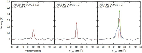
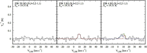
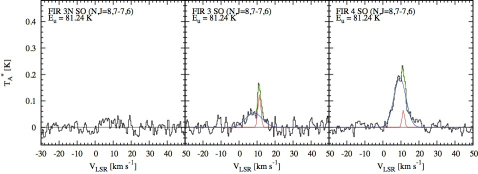
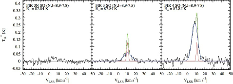
Figure A25: SO spectra

However, the wide components of the SO emission with higher upper energy levels are also seen at FIR 3 (see Fig. A25). Thus, there are two possibilities. First is that the SO emission traces the molecular outflow and the non-detection at FIR 3N of the wide components is due to poor sensitivity. Second is that the SO emission traces the outflow shock and the wide components at FIR 3 trace the outflow shock near the driving source where the outflow gas is being launched. The possible reason for the wide components of only SO being detected at FIR 3 is that the SO emission has higher upper energy levels ($E_{\rm u}$ $>$80 K) and traces the warm region. However, the H₂CS and CH₃OH emission lines with a higher upper energy level more than 80 K have only narrow components at FIR 3. The velocity widths of these narrow components (2.9 km s^-1) are 1.3 times larger than those at FIR 4 (2.3 km s^-1). Thus, it might be true that the wide components could not be detected at FIR 3 due to poor sensitivity.

While the wide components of the normal species, CS and HCN, are detected at the three positions and trace the molecular outflow as described in Sect. 5.1.3, the wide components of their rare isotopic species, C³⁴S and H¹³CN are detected only at FIR 4. To investigate whether the absence of the C³⁴S and H¹³CN wide components at FIR 3N and FIR 3 is due to poor sensitivity or not, we compared the 3$\sigma$ upper limits of the column densities at FIR 3N and FIR 3 with the column density at FIR 4. If the C³⁴S and H¹³CN emission trace the outflow, the wide components should be detected at the three positions. Here, to estimate the 3$\sigma$ upper limits of the column densities, we assume that the velocity widths of the wide components at FIR 3N and FIR 3 are the same as those at FIR 4. The 3$\sigma$ upper limits of the C³⁴S column density with an assumption of $T$ = 20K are estimated to be 7.6$\times$10¹² cm^-2 at FIR 3N and 7.4$\times$10¹² cm^-2 at FIR 3, while the C³⁴S column density of the wide component at FIR 4 is 1.1$\times$10¹³ cm^-2. The 3$\sigma$ upper limits of the H¹³CN column density with an assumption of $T$ = 20K are estimated to be 3.2$\times$10¹³ cm^-2 at FIR 3N and 2.7$\times$10¹³ cm^-2 at FIR 3, while the H¹³CN column density of the wide component at FIR 4 is 6.4$\times$10¹³ cm^-2. The 3$\sigma$ upper limits of C³⁴S and H¹³CN at FIR 3N are plotted above the line of $N_{\rm mol}$(FIR 3N)=$\frac{N_{\rm H^{13}CO^{+}}({\rm FIR\ 3N})}{N_{\rm H^{13}CO^{+}}({\rm FIR\ 4})}$$N_{\rm mol}$(FIR 4), indicating that the non-detection of the C³⁴S and H¹³CN wide components at FIR 3N might be due to the poor sensitivity. However, the 3$\sigma$ upper limits of C³⁴S and H¹³CN at FIR 3 are plotted below the line of $N_{\rm mol}$(FIR 3)=$\frac{N_{\rm H^{13}CO^{+}}({\rm FIR\ 3})}{N_{\rm H^{13}CO^{+}}({\rm FIR\ 4})}$$N_{\rm mol}$(FIR 4), indicating the non-detection of C³⁴S and H¹³CN wide components at FIR 3 is not due to the poor sensitivity. It is quite unlikely that the C³⁴S and H¹³CN wide components trace the outflow because these components were not detected at FIR 3 in spite of the sufficient sensitivity we take into account for the sensitivity. Thus, the C³⁴S and H¹³CN wide components at FIR 4 are likely to trace the outflow shock.

5.1.5 Possible shock tracers

The velocity widths of the narrow components of the HCS⁺, H₂CO, HNCO, and CH₃CHO emission toward FIR 4 are 1.5 times or more as larger as those at FIR 3N and FIR 3 and those of the ambient dense-gas tracers. The velocity widths of HCS⁺, H₂CO, HNCO, and CH₃CHO emission lines in FIR 4 have 3.01, 3.84, 3.15, and 2.34–3.81 km s^-1, respectively, while the mean velocity width of the ambient dense-gas tracers is 2.1$\pm$0.7 km s^-1. Thus, these emission lines might have a wide component at FIR 4 and might trace the outflow shock. If the wide component is not seen due to poor sensitivity, the single Gaussian fitting gives a broader line width. In fact, the signal-to-noise ratios of the emission are too low to separate the two components. Although the narrow components of the HDCO (5_1,4–4_1,3) emission are detected at FIR 3 and FIR 4, we consider HDCO as a possible shock tracer for the following reasons. These intensities and velocity widths are 0.100 K in $T_{\rm A}^{*}$ (S/N=3.0) and 2.93 km s^-1, respectively, at FIR 3: 0.099 K in $T_{\rm A}^{*}$ (S/N=4.1) and 3.45 km s^-1, respectively, at FIR 4. The velocity widths at FIR 3 and FIR 4 are 1.5 times or more as broad as those of the ambient dense-gas tracers. As we described in Sect. 4.5, the non-detection of HDCO at FIR 3N is not due to the poor sensitivity. This emission might trace the outflow shock at the launching point of the FIR 3 outflow and at the interface between the FIR 3 outflow and the dense gas associated with FIR 4.

5.2 Shock vs hot core chemistry

On the basis of the molecular abundances, we discuss two possible origins for the chemical enrichment at FIR 4. One is the shock chemistry caused by the collision between the outflow from FIR 3 and the dense clump at FIR 4, and the other is the hot-core chemistry as suggested by Ceccarelli et al. (2010), Kama et al. (2013), Kama et al. (2014), and López-Sepulcre et al. (2013).

First, we compare the molecular abundances in FIR 4 with those in L 1157 B1 ($d$ = 440 pc, Viotti, 1969) which is a well-studied outflow-shocked region (Avery & Chiao, 1996; Bachiller et al., 2001; Sugimura et al., 2011). In L 1157 B1, the molecular outflow driven from IRAS 20386+6751 interacts with the ambient cloud. The total luminosities of the outflow driving sources, OMC 2-FIR 3 and L 1157, are estimated to be 300 and 4 $L_{\odot}$, respectively (Adams et al., 2012; Mundy et al., 1986). The momentum ($P$) of both the blue and red lobes of FIR 3 (2.4 $M_{\odot}$ km s^-1), however, is comparable to that of L 1157 (4.7 $M_{\odot}$ km s^-1), where no corrections are made for projection angles of the outflows (Aso et al., 2000; Bachiller et al., 2001).

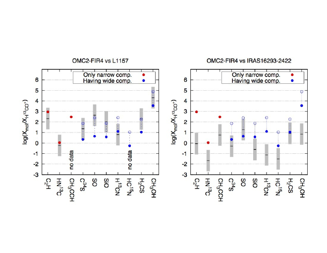
Figure 9: Comparison of the fractional abundances relative to that of H¹³CO⁺ for the 10 molecules among OMC 2-FIR 4, L 1157 B1, and IRAS 16293-2422. The horizontal black bars show the molecular abundances of the molecule at L 1157 B1 and IRAS 16293-2422. The gray boxes show the uncertainties of one order of magnitude in the fractional abundances estimated for L 1157 B1 and IRAS 16293-2422 (Bachiller & Perez Gutierrez, 1997; Schöier et al., 2002). The red circle shows the abundance of the molecule whose spectrum has a single narrow component at FIR 4. The blue circle shows the abundance of the molecule whose spectrum has narrow and wide components at FIR 4. The lower limit values (blue filled circles) for CH₃OH, SO, H₂CS, SiO, C³⁴S, HC¹⁵N, and H¹³CN in FIR 4 are the abundances derived on the assumption that the source size is 19$\arcsec$ for all the detected transitions of each molecule. The upper limit values (blue open circles) are the abundances corrected for the beam dilution assuming that the source size is 3$\arcsec$.

Figure 9 (Left) shows a comparison of the molecular fractional abundances relative to H¹³CO⁺ between FIR 4 and L 1157 B1. Here, we adopted the abundances for L 1157 B1 from Bachiller & Perez Gutierrez (1997). The abundances for FIR 4 are the sum of the abundances for the narrow and wide components. We estimate the H¹³CN and HN¹³C abundances from the HCN and HNC abundances on the assumption that [HCN]/[H¹³CN]=[¹²CO]/[¹³CO], [HNC]/[HN¹³C]=[¹²CO]/[¹³CO], and [¹²CO]/[¹³CO]=90.9 (Bachiller & Perez Gutierrez, 1997). The abundances of C₂H, H¹³CN, HN¹³C, and CH₃OH in FIR 4 are similar to those in L 1157 B1. On the other hand, the abundances of C³⁴S, SiO, SO, and H₂CS in FIR 4 are one order of magnitude lower than those in L 1157 B1. These significant differences are, however, likely due to the beam dilution effect, as described in Sect. 4.4. The corrected abundances in FIR 4 come to agree with the abundances in L 1157 B1, as shown in Fig. 9 (Left). Hence, the chemical composition of FIR 4 could be caused by the outflow shock.

Next, we compare the molecular abundances in FIR 4 with those in IRAS 16293-2422 ($d$ = 160 pc: Whittet, 1974) which is a well-studied low-mass hot corino. The total luminosity of IRAS 16293-2422 is comparable to that of FIR 4 (50 $L_{\odot}$ for FIR 4 by Adams et al. 2012 and 27 $L_{\odot}$ for IRAS 16293-2422 by Mundy et al. 1986). Here, we adopted the molecular abundances in IRAS 16293-2422 from Schöier et al. (2002). Figure 9 (right) shows a comparison of the molecular fractional abundances relative to H¹³CO⁺ between FIR 4 and IRAS 16293-2422. In the comparison, the fractional abundances of C³⁴S, SO and H₂CS are similar to each other in the two regions within one order of magnitude. On the other hand, the abundances of C₂H, HN¹³C, CH₃CCH, SiO, H¹³CN, HC¹⁵N, and CH₃OH in FIR 4 are one order of magnitude higher than those in IRAS 16293-2422. Here, we note that the abundances of the shock tracer molecules in Schöier et al. (2002) seem to be affected by the beam dilution effect, because Chandler et al. (2005) revealed that shock tracer molecules have compact structures in IRAS 16293-2422.

Although we cannot exclude a possibility that the chemical enrichment in FIR 4 is caused by the hot core chemistry, the chemical compositions in FIR 4 are more similar to those in L 1157 B1 than those in IRAS 16293-2422. Although we have detected 120 molecular lines, it is still controversial whether the chemical enrichment in FIR 4 is caused by the outflow shock or by the hot core chemistry from the viewpoint of the molecular abundances. However, results of previous observations with angular resolutions of 3–5$\arcsec$ support the scenario that the outflow shock is the origin of the chemical enrichment in FIR 4 for the following reasons. First, the SiO emission is distributed at the interface between the outflow driven from FIR 3 and the dense gas associated with FIR 4 (see Fig. 1). Second, in the position-velocity diagram, the SiO emission is located at the tip of the CO outflow emission, suggesting that the SiO emission is kinematically related with the FIR 3 outflow (see Fig. 8 in Shimajiri et al., 2008). Third, the distribution of the SiO emission does not coincide with that of the dusty cores traced in the 3.3-mm dust continuum emission. Furthermore, any infrared sources, i.e., the driving sources of the hot core chemistry, are not associated with the dusty cores (Adams et al., 2012).

To firmly unveil the origin of the chemical enrichment in FIR 4, observations with an angular resolution of $<$ $\sim$3$\arcsec$ are urgent. If the molecules interpreted as shock tracer are found to be distributed at the interface between the FIR 3 outflow and the dense clump in FIR 4, the chemical enrichment in FIR 4 comes to be caused by the outflow shock. If the molecules are found to be concentrated at the hot core candidate, the hot core chemistry is dominated.

6 Summary

Using the Nobeyama 45 m and ASTE telescopes, we have conducted first line-survey observations at 82–106 GHz and 335–355 GHz toward an outflow-shocked region, FIR 4. To deeply characterize the chemistry in FIR 4, we have observed the two additional sources of FIR 3, an outflow driving source and FIR 3N, an outflow lobe without shock. The main results are summarized as follows:

The main results are summarized as follows.

1. Our 3-mm and 850-$\mu$m line surveys have identified 120 lines and 20 species including CH₃CCH, CH₃CHO, and C₃H₂ as well as S-bearing molecules such as H₂CS, SO, and HCS⁺. In addition, 11 rare isotopic species including ¹³C-bearing, ¹⁵N-bearing, ¹⁷O-bearing, ¹⁸O-bearing, ³⁴S-bearing, and deuterated species are detected. We have found that the line profiles of the molecules can be classified into the two types: one Gaussian component with a narrow ($<$ 3 km s^-1) velocity width and two Gaussian components with narrow and wide ($>$ 3 km s^-1) velocity widths.

2. We have estimated the rotation temperatures of the detected molecules with multiple transitions by the rotation diagram method. The rotation temperatures of C₂H and H¹³CO⁺ having only one narrow component are found to be 12.5$\pm$1.4 K. On the other hand, the rotation temperatures of the wide components are estimated to be 20–70 K, suggesting that the components trace the outflow and/or the outflow shock.

3. On the basis of the spatial distributions, velocity widths, and rotation temperatures of the detected emission lines, we discussed what physical and chemical conditions the detected molecular emission lines trace. The narrow components of the CN, C¹⁷O, C₂H, HNC, HN¹³C, H¹³CO⁺, N₂H⁺, c-C₃H₂, and CH₃CN emission are detected at the three positions and the rotation temperatures of C₂H and H¹³CO⁺ are estimated to be 12.5$\pm$1.4 K. Thus, these are considered to trace the ambient dense gas. The narrow components of the ¹³CS, H¹⁵NC, HC¹⁸O⁺, NH₂D, CH₃CCH emission are detected at one or two positions. Those velocity widths are similar to those of the ambient dense-gas tracers. Thus, the emission is likely to trace the ambient dense gas. The wide components of the CO, CS, HCN, and HCO⁺ emission are detected at the three positions and likely trace the molecular outflow. The wide components of the C³⁴S, SO, SiO, H¹³CN, HC¹⁵N, H${}_{2}^{13}$CO, H₂CS, HC₃N, and CH₃OH emission are detected only at FIR 4 with the high rotation temperatures of 20–70 K and likely trace the outflow shock. Although the HCS⁺, H₂CO, HDCO, HNCO, and CH₃CHO line profiles consist of one narrow Gaussian component, these velocity widths are twice or more broader than those of the ambient dense-gas tracers. Thus, the emission lines may have a wide component tracing the outflow shock.

4. We have compared the molecular fractional abundances relative to H¹³CO⁺ in FIR 4 with those in the outflow-shocked region, L 1157 B1, and the hot core, IRAS 16293-2422. Although we cannot exclude a possibility that the chemical enrichment in FIR 4 is caused by the hot core chemistry, the chemical compositions in FIR 4 are more similar to those in L 1157 B1 than those in IRAS 16293-2422. It is still controversial whether the chemical enrichment in FIR 4 is caused by the outflow shock or not.

FIR 4 ($d$ = 400 pc) is one of the nearest outflow-shocked regions and we have revealed that FIR 4 is a chemically rich source. To reveal the nature and origin of the chemical enrichment and the relationship between the chemical and physical conditions, mapping observations with a higher angular resolution of $<<$ 3″are crucial. If the molecules of the possible-shock tracers are enhanced by the outflow shock, the emission is expected to be distributed at the interface between the FIR 3 outflow and the dense gas associated with FIR 4.

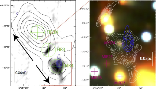
Figure 1: Left: three observed positions (green crosses) for FIR 3N, 3, and 4 in the line-survey observations. The circles mean our beam size in HPBW. The black contours show the distribution of the ¹²CO (3–2) outflow gas from FIR 3 and the outflow direction is indicated by the arrows. The blue contours and the gray-scale map show the SiO (2–1) line and 3.3 mm dust continuum emission, respectively. Right: Magnification of the FIR 3 and 4 regions. The distributions of the SiO (2–1) line (blue contours) and 3.3 mm dust continuum (white contours) emission are superposed on the 2MASS color map in $J$, $H$, and $K$ bands. The crosses show the positions of the mid-infrared sources, MIR 24 to 27.

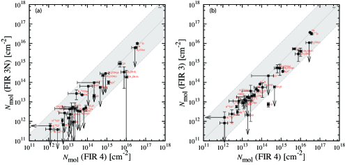
Figure 7: Comparisons of the column densities for the 33 molecules (a) between FIR 3N and FIR 4 and (b) between FIR 3 and FIR 4. The gray lines indicate $N_{\rm mol}$(FIR3N)=$N_{\rm H^{13}CO^{+}}$(FIR3N)/$N_{\rm H^{13}CO^{+}}$(FIR4)$\times$$N_{\rm mol}$(FIR4) in panel (a) and $N_{\rm mol}$(FIR3)=$N_{\rm H^{13}CO^{+}}$(FIR3)/$N_{\rm H^{13}CO^{+}}$(FIR4)$\times$$N_{\rm mol}$(FIR4) in panel (b), and the gray areas show deviations from the lines by a factor 10.

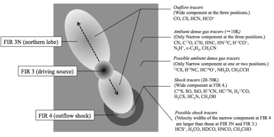
Figure 8: Schematic illustration of the relationship between the physical environment and the chemical composition.

Table 1: Observed Positions and Flux Densities at FIR 3N, 3, and 4

	R.A.	Dec.	Physical environment	$F_{\rm 1.1mm}$†	$N_{\rm H2}$∗	$N_{\rm H2}$∗∗
	(J2000)	(J2000)		[Jy beam-1]	[$\times$ 1022 cm-2]	[$\times$ 1022 cm-2]
FIR 3N	5:35:28.7	-5:09:15.6	Northern lobe of the FIR 3 outflow	1.25	12.2 ($T_{\rm d}$=10.2 K)	2.1 ($T_{\rm d}$=54 K)
FIR 3	5:35:27.6	-5:09:34.0	Outflow driving source	3.79	26.9 ($T_{\rm d}$=13.8 K)	6.6 ($T_{\rm d}$=54 K)
FIR 4	5:35:26.8	-5:09:57.4	Outflow shock	5.95	45.0 ($T_{\rm d}$=13.0 K)	10.0 ($T_{\rm d}$=56 K)

Table 2: Observational Parameters

Telescope/Receiver	NRO 45 m/T100	ASTE/CATS345
$T_{\rm sys}$	150–200 K	200–500 K
Frequency range	82–106 GHz	335–355 GHz
Frequency resolution	488.2 kHz	500.0 kHz
Velocity resolution (at 100/345 GHz)	1.5 km s-1	0.5 km s-1
Beam size (at 100/345 GHz)	15.1$\arcsec$	19.7$\arcsec$

Table 3: Rms Noise Levels in $T_{\rm A}^{*}$ at FIR 3N, 3, and 4

Freq.	FIR 3N	FIR 3	FIR 4
82–86 GHz	40.8 mK	20.8 mK	17.8 mK
86–90 GHz	17.6 mK	18.8 mK	13.5 mK
90–94 GHz	26.8 mK	26.0 mK	17.9 mK
94–98 GHz	27.9 mK	14.8 mK	12.1 mK
98–102 GHz	10.8 mK	13.3 mK	9.9 mK
102–106 GHz	20.8 mK	20.7 mK	13.9 mK
Mean (82–106 GHz)	24.1$\pm$10.3 mK	19.1$\pm$4.6 mK	14.2$\pm$3.2 mK
335–339 GHz	20.9 mK	33.2 mK	23.9 mK
339–343 GHz	21.1 mK	22.1 mK	20.2 mK
343–347 GHz	34.9 mK	32.9 mK	27.0 mK
347–351 GHz	18.6 mK	23.3 mK	20.6 mK
351–355 GHz	37.0 mK	37.9 mK	42.6 mK
Mean (335–355 GHz)	26.5$\pm$8.7 mK	29.9$\pm$6.9 mK	26.9$\pm$9.2 mK

Table 4: Number of the Detected Molecular Lines at FIR 3N, 3, and 4

	Num. of molecular lines	Num. of the most abundant isotopic species	Num. of the rare isotopic species
FIR 3N	53	14	5
FIR 3	100	17	10
FIR 4	119	20	12

Table 5: Detected Molecules toward FIR 3N, 3, and 4, and Relationship between the Physical Environment and the Chemical Composition

Species	FIR 3N		FIR 3		FIR 4		Physical environment
	Narrow	Wide	Narrow	Wide	Narrow	Wide
CN	$\circ$	$\cdots$	$\circ$	$\cdots$	$\circ$	$\cdots$	ambient dense gas
C17O	$\circ$	$\cdots$	$\circ$	$\cdots$	$\circ$	$\cdots$	ambient dense gas
C2H	$\circ$	$\cdots$	$\circ$	$\cdots$	$\circ$	$\cdots$	ambient dense gas
HNC	$\circ$	$\cdots$	$\circ$	$\cdots$	$\circ$	$\cdots$	ambient dense gas
HN13C	$\circ$	$\cdots$	$\circ$	$\cdots$	$\circ$	$\cdots$	ambient dense gas
H13CO+	$\circ$	$\cdots$	$\circ$	$\cdots$	$\circ$	$\cdots$	ambient dense gas
N2H+	$\circ$	$\cdots$	$\circ$	$\cdots$	$\circ$	$\cdots$	ambient dense gas
c-C3H2	$\circ$	$\cdots$	$\circ$	$\cdots$	$\circ$	$\cdots$	ambient dense gas
CH3CN	$\circ$	$\cdots$	$\circ$	$\cdots$	$\circ$	$\cdots$	ambient dense gas
13CS	$\cdots$	$\cdots$	$\circ$	$\cdots$	$\circ$	$\cdots$	(possible) ambient dense gas
H15NC	$\circ$	$\cdots$	$\cdots$	$\cdots$	$\circ$	$\cdots$	(possible) ambient dense gas
HC18O+	$\cdots$	$\cdots$	$\circ$	$\cdots$	$\cdots$	$\cdots$	(possible) ambient dense gas
NH2D	$\cdots$	$\cdots$	$\cdots$	$\cdots$	$\circ$	$\cdots$	(possible) ambient dense gas
CH3CCH	$\cdots$	$\cdots$	$\circ$	$\cdots$	$\circ$	$\cdots$	(possible) ambient dense gas
CO	$\circ$	$\circ$	$\circ$	$\circ$	$\circ$	$\circ$	molecular outflow
CS	$\circ$	$\circ$	$\circ$	$\circ$	$\circ$	$\circ$	molecular outflow
HCN	$\circ$	$\circ$	$\circ$	$\circ$	$\circ$	$\circ$	molecular outflow
HCO+	$\circ$	$\circ$	$\circ$	$\circ$	$\circ$	$\circ$	molecular outflow
C34S	$\cdots$	$\cdots$	$\circ$	$\cdots$	$\circ$	$\circ$	outflow shock
SO	$\circ$	$\cdots$	$\circ$	$\circ$	$\circ$	$\circ$	outflow shock
SiO	$\cdots$	$\cdots$	$\cdots$	$\cdots$	$\circ$	$\circ$	outflow shock
H13CN	$\circ$	$\cdots$	$\circ$	$\cdots$	$\circ$	$\circ$	outflow shock
HC15N	$\cdots$	$\cdots$	$\circ$	$\cdots$	$\circ$	$\circ$	outflow shock
H${}_{2}^{13}$CO	$\circ$	$\cdots$	$\circ$	$\cdots$	$\circ$	$\circ$	outflow shock
H2CS	$\circ$	$\cdots$	$\bullet$	$\cdots$	$\circ$	$\circ$	outflow shock
HC3N	$\circ$	$\cdots$	$\circ$	$\cdots$	$\circ$	$\circ$	outflow shock
CH3OH	$\circ$	$\cdots$	$\bullet$	$\cdots$	$\circ$	$\circ$	outflow shock
HCS+	$\cdots$	$\cdots$	$\cdots$	$\cdots$	$\bullet$	$\cdots$	(possible) outflow shock
H2CO	$\cdots$	$\cdots$	$\cdots$	$\cdots$	$\bullet$	$\cdots$	(possible) outflow shock
HDCO	$\cdots$	$\cdots$	$\bullet$	$\cdots$	$\bullet$	$\cdots$	(possible) outflow shock or (possible) molecular outflow a
HNCO	$\cdots$	$\cdots$	$\circ$	$\cdots$	$\bullet$	$\cdots$	(possible) outflow shock
CH3CHO	$\cdots$	$\cdots$	$\circ$	$\cdots$	$\bullet$	$\cdots$	(possible) outflow shock

Table 6: Optical Depth

			$Narrow\ comp.$			$Wide\ comp.$
Molecule	Rarer isotopic species	Transition	FIR 3N	FIR 3	FIR 4	FIR 3N	FIR 3	FIR 4
HCO+	H13CO+	$J$=1–0	9.7	7.1	8.6	$\cdots$
CS	C34S	$J$=2–1	$\cdots$	0.4	2.1	$\cdots$	$\cdots$	0.9
CS	C34S	$J$=7–6	$\cdots$	1.0	$<<$ 1	$\cdots$	$\cdots$	0.7
HCN	H13CN	$J$=1–0,$F$=1–1	9.1	8.5	10.7	$\cdots$	$\cdots$	37.7
HCN	H13CN	$J$=1–0,$F$=2–1	4.8	5.4	8.1	$\cdots$	$\cdots$	26.7
HCN	H13CN	$J$=1–0,$F$=0–1	4.9	3.9	4.3	$\cdots$	$\cdots$	12.8
HCN	H13CN	$J$=4–3	$\cdots$	5.9	7.1	$\cdots$	$\cdots$	5.7
HNC	HN13C	$J$=1–0	3.1	4.5	6.2	$\cdots$

Table 7: Rotational Temperatures, Column Densities, and Fractional Abundances of the Detected Molecules at FIR 3N, 3, and 4^∗

Species	Position	$Narrow\ comp.$		$Wide\ comp.$
		$T_{\rm rot}$ [K]†	$N_{\rm mol}$ [cm-2]‡	$T_{\rm rot}$ [K]†	$N_{\rm mol}$ [cm-2]†	$N_{\rm mol}$ total	$X_{\rm mol}$‡ ($T_{\rm d}$ = $T_{\rm rot}$ (H13CO+))	$X_{\rm mol}$‡ ($T_{\rm d}$ = $T_{\rm CO\ peak}$)
	FIR 3N	$\cdots$	$<$ 1.5$\times$1012 ($T$ = 10 K)	$\cdots$
C34S	FIR 3	17.7$\pm$5.0	(8.7$\pm$2.6)$\times$1012	$\cdots$			(0.3$\pm$0.1)$\times$10-10	(1.3$\pm$0.4)$\times$10-10
	FIR 4	10.7$\pm$2.6	(9.4$\pm$1.8)$\times$1012	27.0$\pm$16.9	(1.1$\pm$0.8)$\times$1013	(1.1$\pm$0.2)$\times$1013	(2.4$\pm$0.4)$\times$10-11	(1.1$\pm$0.2)$\times$10-10
	FIR 3N	$\cdots$	$<$ 9.4$\times$1011 ($T$ = 20 K)	$\cdots$
SiO	FIR 3	$\cdots$	$<$ 2.1$\times$1012 ($T$ = 20 K)	$\cdots$
	FIR 4	19.4$\pm$4.9	(3.3$\pm$1.4)$\times$1012	24.6$\pm$6.8	(1.6$\pm$0.5)$\times$1013	(1.9$\pm$0.5)$\times$1013	(4.2$\pm$1.1)$\times$10-11	(1.9$\pm$0.5)$\times$10-10
	FIR 3N	$\cdots$	(2.0$\pm$0.4)$\times$1013 ($T$ = 20 K)	$\cdots$
SO	FIR 3	22.3$\pm$2.1	(7.4$\pm$1.9)$\times$1013	$\cdots$			(0.3$\pm$0.1)$\times$10-9	(1.1$\pm$0.3)$\times$10-9
	FIR 4	21.1$\pm$2.8	(4.7$\pm$1.8)$\times$1013	39.8 $\pm$5.2	(1.7$\pm$0.3)$\times$1014	(2.2$\pm$0.3)$\times$1014	(4.9$\pm$0.7)$\times$10-10	(2.2$\pm$0.3)$\times$10-9
	FIR 3N	11.5 $\pm$1.5	(9.2$\pm$3.0) $\times$1014	$\cdots$			(0.8$\pm$0.3)$\times$10-8	(4.4$\pm$0.4)$\times$10-8
C2H	FIR 3	14.3 $\pm$0.6	(5.3$\pm$0.4) $\times$1015	$\cdots$			(2.0$\pm$0.2)$\times$10-8	(8.0$\pm$0.6)$\times$10-8
	FIR 4	12.3 $\pm$1.0	(4.7$\pm$0.9) $\times$1015	$\cdots$			(1.0$\pm$0.2)$\times$10-8	(4.7$\pm$0.9)$\times$10-8
	FIR 3N	$\cdots$	$<$ 4.3 $\times$ 1012 ($T$ = 10 K)	$\cdots$
H13CN	FIR 3	12.2$\pm$0.5	(3.8$\pm$0.3)$\times$1013	$\cdots$			(1.4$\pm$0.1)$\times$10-10	(5.8$\pm$0.5)$\times$10-10
	FIR 4	8.7$\pm$0.3	(3.3$\pm$0.3)$\times$1013	20.2 $\pm$ 0.4	(3.1$\pm$0.1)$\times$1013	(6.4$\pm$0.3)$\times$1013	(1.4$\pm$0.1)$\times$10-10	(6.4$\pm$0.3)$\times$10-10
	FIR 3N	$\cdots$	$<$ 3.8$\times$1011 ($T$ = 10 K)	$\cdots$
HC15N	FIR 3	10.4$\pm$2.3	(2.4$\pm$1.5)$\times$1012	$\cdots$			(0.9$\pm$0.6)$\times$10-11	(3.6$\pm$2.3)$\times$10-11
	FIR 4	9.5$\pm$2.5	(2.9$\pm$0.9)$\times$1012	$\cdots$			(0.6$\pm$0.2)$\times$10-11	(2.9$\pm$0.9)$\times$10-11
	FIR 3N	10.2$\pm$2.4	(1.1$\pm$0.3)$\times$1012	$\cdots$			(8.8$\pm$2.1)$\times$10-12	(5.2$\pm$1.4)$\times$10-11
H13CO+	FIR 3	13.8$\pm$1.0	(5.7$\pm$0.7)$\times$1012	$\cdots$			(2.1$\pm$0.3)$\times$10-11	(8.6$\pm$1.1)$\times$10-11
	FIR 4	13.0$\pm$0.6	(5.1$\pm$0.4)$\times$1012	$\cdots$			(1.1$\pm$0.1)$\times$10-11	(5.1$\pm$0.4)$\times$10-11
	FIR 3N	$\cdots$	$<$ 6.7$\times$1011 ($T$ = 10 K)	$\cdots$
HN13C	FIR 3	10.6$\pm$3.0	(3.0$\pm$0.9)$\times$1012	$\cdots$			(1.1$\pm$0.3)$\times$10-11	(4.5$\pm$1.4)$\times$10-11
	FIR 4	9.8$\pm$0.8	(5.6$\pm$0.6)$\times$1012	$\cdots$			(1.2$\pm$0.1)$\times$10-11	(5.6$\pm$0.6)$\times$10-11
	FIR 3N	$\cdots$	$<$ 2.3$\times$1012 ($T$ = 20 K)	$\cdots$
H2CS (ortho)	FIR 3	24.0$\pm$7.6	(1.3$\pm$0.8)$\times$1013	$\cdots$			(0.5$\pm$0.3)$\times$10-10	(2.0$\pm$1.2)$\times$10-10
	FIR 4	20.7$\pm$4.9	(1.3$\pm$0.5)$\times$1013	$\cdots$			(0.3$\pm$0.1)$\times$10-10	(1.3$\pm$0.5)$\times$10-10
	FIR 3N	$\cdots$	$<$ 3.3$\times$1012 ($T$ = 40 K)	$\cdots$
H2CS (para)	FIR 3	46.1$\pm$5.5	(2.2$\pm$0.4)$\times$1013	$\cdots$			(0.8$\pm$0.2)$\times$10-10	(3.3$\pm$0.6)$\times$10-10
	FIR 4	21.6$\pm$0.8	(4.1$\pm$0.6)$\times$1013	$\cdots$			(0.9$\pm$0.1)$\times$10-10	(4.1$\pm$0.6)$\times$10-10
	FIR 3N	$\cdots$	$<$ 3.5$\times$1012 ($T$ = 40 K)	$\cdots$
CH3CN (ortho)∗∗	FIR 3	$\cdots$	(2.0$\pm$0.9)$\times$1013 ($T$ = 40 K)	$\cdots$
	FIR 4	54.8$\pm$46.5	(3.1$\pm$1.0)$\times$1013	$\cdots$			(0.7$\pm$0.2)$\times$10-10	(3.1$\pm$1.0)$\times$10-10
	FIR 3N	$\cdots$	(4.5$\pm$4.4)$\times$1012 ($T$ = 40 K)	$\cdots$
CH3CN (para)††	FIR 3	$\cdots$	(1.1$\pm$0.5)$\times$1013 ($T$ = 40 K)	$\cdots$
	FIR 4	34.5$\pm$ 37.9	(1.5$\pm$1.3)$\times$1013	$\cdots$			(3.4$\pm$2.8)$\times$10-11	(1.5$\pm$1.3)$\times$10-10
	FIR 3N	26.0$\pm$21.3	(1.9$\pm$2.3)$\times$1014	$\cdots$			(1.6$\pm$1.9)$\times$10-9	(9.0$\pm$0.1)$\times$10-9
CH3OH A	FIR 3	57.7$\pm$11.7	(4.0$\pm$1.8)$\times$1015	$\cdots$			(0.2$\pm$ 0.1)$\times$10-7	(6.1$\pm$2.3)$\times$10-8
	FIR 4	46.2$\pm$6.9	(3.1$\pm$1.2)$\times$1015	66.2$\pm$6.6	(7.0$\pm$1.4)$\times$1015	(1.0$\pm$0.2)$\times$1016	(2.2$\pm$0.4)$\times$10-8	(1.0$\pm$0.2)$\times$10-7
	FIR 3N	$\cdots$	(3.4$\pm$2.9)$\times$1014 ($T$ = 20 K)	$\cdots$
CH3OH E	FIR 3	32.4$\pm$11.2	(2.9$\pm$1.7)$\times$1015	$\cdots$			(1.1$\pm$0.6)$\times$10-8	(4.4$\pm$2.6)$\times$10-8
	FIR 4	25.0$\pm$3.2	(2.4$\pm$0.8)$\times$1015	46.0$\pm$12.3	(5.3$\pm$2.2)$\times$1015	(7.7$\pm$2.3)$\times$1015	(1.7$\pm$0.5)$\times$10-8	(7.7$\pm$2.3)$\times$10-8
	FIR 3N	$\cdots$	$<$ 2.3$\times$1014 ($T$ = 40 K)	$\cdots$
CH3CCH (ortho)	FIR 3	$\cdots$	(5.6$\pm$2.5)$\times$1014 ($T$ = 40 K)	$\cdots$
	FIR 4	32.7$\pm$3.5	(6.4 $\pm$1.0)$\times$1014	$\cdots$			(1.4$\pm$0.2)$\times$10-9	(6.4$\pm$1.0)$\times$10-9
	FIR 3N	$\cdots$	$<$2.9$\times$1014 ($T$ = 40 K)	$\cdots$
CH3CCH (para)††	FIR 3	$\cdots$	(5.4$\pm$3.1)$\times$1014 ($T$ = 40 K)	$\cdots$
	FIR 4	54.1$\pm$40.0	(8.6$\pm$4.1)$\times$1014	$\cdots$			(1.9$\pm$0.9)$\times$10-9	(8.6$\pm$4.1)$\times$10-9

Table 8: Rotational Temperatures, Column Densities, and Fractional Abundances of the Detected Molecules at FIR 3N, 3, and 4, which are estimated on the assumption of $f$=1

Species	Position	$Narrow\ comp.$		$Wide\ comp.$
		$T_{\rm rot}$ [K]†	$N_{\rm mol}$ [cm-2]‡	$T_{\rm rot}$ [K]†	$N_{\rm mol}$ [cm-2]†	$N_{\rm mol}$ total	$X_{\rm mol}$‡ ($T_{\rm d}$ = $T_{\rm rot}$ (H13CO+))	$X_{\rm mol}$‡ ($T_{\rm d}$ = $T_{\rm CO\ peak}$)
	FIR 3N	$\cdots$	$<$1.5$\times$1012 ($T$ = 10 K)	$\cdots$
C34S	FIR 3	16.0$\pm$4.1	(4.4$\pm$1.3)$\times$1012	$\cdots$			(1.6$\pm$0.5)$\times$10-11	(6.7$\pm$2.0)$\times$10-11
	FIR 4	10.1$\pm$2.3	(5.5$\pm$1.1)$\times$1012	23.6$\pm$12.9	(5.6$\pm$4.3)$\times$1012	(1.1$\pm$0.4)$\times$1013	(2.4$\pm$0.9)$\times$10-11	(1.1$\pm$0.4)$\times$10-10
	FIR 3N	$\cdots$	$<$9.4$\times$1011 ($T$ = 20 K)	$\cdots$
SiO	FIR 3	$\cdots$	$<$1.0$\times$1012 ($T$ = 20 K)	$\cdots$
	FIR 4	18.8$\pm$ 4.6	(1.8$\pm$0.8)$\times$1012	23.6 $\pm$6.3	(8.5$\pm$2.9)$\times$1012	(1.0$\pm$0.3)$\times$1013	(2.2$\pm$0.7)$\times$10-11	(1.0$\pm$0.3)$\times$10-10
	FIR 3N	$\cdots$	(2.0$\pm$0.4)$\times$1013 ($T$ = 20 K)	$\cdots$
SO	FIR 3	20.9$\pm$1.6	(3.7$\pm$0.8)$\times$1013	$\cdots$			(1.4$\pm$0.3)$\times$10-10	(5.6$\pm$1.2)$\times$10-10
	FIR 4	20.0$\pm$2.7	(2.6$\pm$1.1)$\times$1013	36.1$\pm$5.1	(9.1$\pm$2.2)$\times$1013	(1.2$\pm$0.2)$\times$1014	(2.7$\pm$0.4)$\times$10-11	(1.2$\pm$0.2)$\times$10-9
	FIR 3N	11.5$\pm$1.5	(9.2$\pm$3.0)$\times$1014	$\cdots$			(7.5$\pm$2.5)$\times$10-9	(4.4$\pm$ 1.4)$\times$10-8
C2H	FIR 3	13.7$\pm$0.5	(2.5$\pm$0.2)$\times$1015	$\cdots$			(9.4$\pm$0.7)$\times$10-9	(3.8$\pm$0.3)$\times$10-8
	FIR 4	11.8$\pm$0.9	(2.5$\pm$0.5)$\times$1015	$\cdots$			(5.6$\pm$1.1)$\times$10-9	(2.5$\pm$0.5)$\times$10-8
	FIR 3N	$\cdots$	$<$4.3$\times$1012 ($T$ = 10 K)	$\cdots$
H13CN	FIR 3	11.7$\pm$0.5	(1.8$\pm$0.2)$\times$1013	$\cdots$			(6.7$\pm$0.6)$\times$10-11	(2.7$\pm$0.3)$\times$10-10
	FIR 4	8.4$\pm$0.3	(1.8$\pm$0.1)$\times$1013	19.0$\pm$0.3	(15.9$\pm$0.3) $\times$ 1012	(3.4$\pm$0.1)$\times$1013	(7.6$\pm$0.2)$\times$10-11	(3.4$\pm$0.1)$\times$10-10
	FIR 3N	$\cdots$	$<$3.8$\times$1011 ($T$ = 10 K)	$\cdots$
HC15N	FIR 3	10.0$\pm$2.2	(1.1$\pm$0.7)$\times$1012	$\cdots$			(0.4$\pm$0.3)$\times$10-11	(1.7$\pm$1.1)$\times$10-11
	FIR 4	9.2$\pm$2.3	(1.5$\pm$0.5)$\times$1012	$\cdots$			(0.3$\pm$0.1)$\times$10-11	(1.5$\pm$0.5)$\times$10-11
	FIR 3N	10.2$\pm$2.4	(1.1$\pm$0.3)$\times$1012	$\cdots$			(0.9$\pm$ 0.2)$\times$10-11	(5.2$\pm$ 1.4)$\times$10-11
H13CO+	FIR 3	13.2$\pm$0.9	(2.7$\pm$0.3)$\times$1012	$\cdots$			(1.0$\pm$ 0.1)$\times$10-11	(4.1$\pm$0.5)$\times$10-11
	FIR 4	12.5$\pm$0.6	(2.7$\pm$0.2)$\times$1012	$\cdots$			(6.0$\pm$ 0.4)$\times$10-12	(2.7$\pm$0.2)$\times$10-11
	FIR 3N	$\cdots$	$<$6.7$\times$1011 ($T$ = 10 K)	$\cdots$
HN13C	FIR 3	10.2$\pm$2.8	(1.5$\pm$0.4)$\times$1012	$\cdots$			(0.5$\pm$0.2)$\times$10-11	(2.3$\pm$0.6)$\times$10-11
	FIR 4	9.5$\pm$0.7	(3.0$\pm$0.3)$\times$1012	$\cdots$			(0.7$\pm$0.1)$\times$10-11	(3.0$\pm$0.3)$\times$10-11
	FIR 3N	$\cdots$	$<$2.3$\times$1012 ($T$ = 20 K)	$\cdots$
H2CS (ortho)	FIR 3	22.0$\pm$6.4	(6.7$\pm$4.4)$\times$1012	$\cdots$			(2.5$\pm$1.6)$\times$10-11	(1.0$\pm$0.7)$\times$10-10
	FIR 4	19.4$\pm$4.3	(7.6$\pm$2.8)$\times$1012	$\cdots$			(1.7$\pm$0.6)$\times$10-11	(7.6$\pm$2.8)$\times$10-11
	FIR 3N	$\cdots$	$<$3.3$\times$1012 ($T$ = 40 K)	$\cdots$
H2CS (para)	FIR 3	39.4$\pm$3.5	(1.1$\pm$0.2)$\times$1013	$\cdots$			(4.1$\pm$0.7)$\times$10-11	(1.7$\pm$0.3)$\times$10-10
	FIR 4	20.2$\pm$0.8	(2.4$\pm$0.3)$\times$1013	$\cdots$			(5.4$\pm$0.8)$\times$10-11	(2.4$\pm$0.3)$\times$10-10
	FIR 3N	$\cdots$	$<$3.5 $\times$1012 ($T$ = 40 K)	$\cdots$
CH3CN (ortho)	FIR 3	$\cdots$	(1.1$\pm$0.5)$\times$1013 ($T$ = 40 K)	$\cdots$
	FIR 4	54.8$\pm$46.5	(1.8$\pm$0.6)$\times$1013	$\cdots$			(0.4$\pm$0.1)$\times$10-10	(1.8$\pm$0.6)$\times$10-10
	FIR 3N	$\cdots$	(4.5$\pm$4.1)$\times$1012 ($T$ = 40 K)	$\cdots$
CH3CN (para)††	FIR 3	$\cdots$	(1.1$\pm$0.6)$\times$1013 ($T$ = 40 K)	$\cdots$
	FIR 4	34.5$\pm$37.9	(8.8$\pm$7.2)$\times$1012	$\cdots$			(2.0$\pm$1.6)$\times$10-11	(8.8$\pm$7.2)$\times$10-11
	FIR 3N	26.0$\pm$21.3	(1.9$\pm$2.3)$\times$1014	$\cdots$			(1.6$\pm$1.9)$\times$10-9	(9.0$\pm$11.0)$\times$10-9
CH3OH A	FIR 3	55.2$\pm$11.4	(1.8$\pm$0.9)$\times$1015	$\cdots$			(0.7$\pm$0.3)$\times$10-8	(2.7$\pm$1.4)$\times$10-8
	FIR 4	44.9$\pm$7.0	(1.6$\pm$0.7)$\times$1015	63.9$\pm$6.7	(3.5$\pm$0.8)$\times$1015	(5.1$\pm$1.1)$\times$1015	(1.1$\pm$0.2)$\times$10-8	(5.1$\pm$1.1)$\times$10-8
	FIR 3N	$\cdots$	(3.4$\pm$2.9)$\times$1014 ($T$ = 20 K)	$\cdots$
CH3OH E	FIR 3	28.9$\pm$8.9	(1.3$\pm$0.8)$\times$1015	$\cdots$			(0.5$\pm$0.3)$\times$10-8	(2.0$\pm$1.2)$\times$10-8
	FIR 4	23.2$\pm$2.9	(1.3$\pm$0.4)$\times$1015	41.1$\pm$9.5	(2.5$\pm$1.0)$\times$1015	(3.8$\pm$1.1)$\times$1015	(8.4$\pm$2.4)$\times$10-9	(3.8$\pm$1.1)$\times$10-8
	FIR 3N	$\cdots$	$<$2.3$\times$1014 ($T$ = 40 K)	$\cdots$
CH3CCH (ortho)	FIR 3	$\cdots$	(2.7$\pm$1.2)$\times$1014 ($T$ = 40 K)	$\cdots$
	FIR 4	34.1$\pm$1.6	(3.9$\pm$0.3)$\times$1014	$\cdots$			(0.9$\pm$0.1)$\times$10-9	(3.9$\pm$3.0)$\times$10-9
	FIR 3N	$\cdots$	$<$2.9$\times$1014 ($T$ = 40 K)	$\cdots$
CH3CCH (para)††	FIR 3	$\cdots$	(2.6$\pm$1.5) $\times$1014 ($T$ = 40 K)	$\cdots$
	FIR 4	58.9$\pm$62.0	(5.4$\pm$3.3)$\times$1014	$\cdots$			(1.2$\pm$0.7)$\times$10-9	(5.4$\pm$3.3)$\times$10-9

Table 9: Relationship between the physical environment and the chemical composition

	FIR 3N	FIR 3	FIR 4	Molecules
Ambient dense gas	Narrow	Narrow	Narrow	CN, C17O, C2H, HNC, HN13C,
				H13CO+, N2H+, c-C3H2, CH3CN
Possible ambient dense gas	non-detection	Narrow	Narrow	13CS, CH3CCH
	non-detection	non-detection	Narrow	NH2D
	Narrow	non-detection	Narrow	H15NC
	non-detection	Narrow	non-detection	HC18O+
Outflow	Narrow and Wide	Narrow and Wide	Narrow and Wide	CO, CS, HCN, HCO+
Shock	Narrow	Narrow	Narrow and Wide	C34S, SO, SiO, H13CN, HC15N,
				H${}_{2}^{13}$CO, H2CS, HC3N, CH3OH
Possible Shock	Narrow	Narrow	Narrow (large velocity width)	HCS+, H2CO, HNCO, CH3CHO
	non-detection	Narrow	Narrow (large velocity width)	HDCO

Table 10: Column Densities of the Molecules Detected with Only One Transition at FIR 3N, 3, and 4^∗

Species	Position	$T$ = 10 K	$T$ = 20 K	$T$ = 40 K
		$N_{\rm mol}$	$N_{\rm mol}$	$N_{\rm mol}$
		[cm-2]	[cm-2]	[cm-2]
C34S	FIR 3N	$<$1.5$\times$1012	$<$2.3$\times$1012	$<$4.0$\times$1012
SiO	FIR 3N	$<$6.2$\times$1011	$<$ 9.4$\times$1011	$<$1.6$\times$1012
SiO	FIR 3	$<$1.4$\times$1012	$<$ 2.0$\times$1012	$<$3.6$\times$1012
SO	FIR 3N	(1.2$\pm$0.3)$\times$1013	(2.0$\pm$0.4)$\times$1013	(3.7$\pm$0.8)$\times$1013
H13CN	FIR 3N	$<$4.3$\times$1012	$<$7.6$\times$1012	$<$1.4$\times$1013
HC15N	FIR 3N	$<$3.8$\times$1011	$<$6.6$\times$1011	$<$1.2$\times$1012
HN13C	FIR 3N	$<$6.7$\times$1011	$<$1.2$\times$1012	$<$2.2$\times$1012
H2CS (ortho)	FIR 3N	$<$1.6$\times$1012	$<$2.3$\times$1012	$<$4.9$\times$1012
H2CS (para)	FIR 3N	$<$1.6$\times$1012	$<$2.0$\times$1012	$<$3.3$\times$1012
CH3CN (ortho)	FIR 3N	$<$1.7$\times$1012	$<$1.9$\times$1012	$<$3.5$\times$1012
CH3CN (ortho)	FIR 3	(5.1$\pm$2.2)$\times$1012	(5.7$\pm$2.4)$\times$1012	(1.1$\pm$0.5)$\times$1013
CH3CN (para)	FIR 3N	(20.0$\pm$19.6)$\times$1011	(25.2$\pm$24.7)$\times$1011	(45.0$\pm$44.1)$\times$1011
CH3CN (para)	FIR 3	(9.3$\pm$4.8)$\times$1012	(1.2$\pm$0.6)$\times$1013	(2.1$\pm$1.1)$\times$1013
CH3OH E	FIR 3N	(3.7$\pm$3.2)$\times$1014	(3.4$\pm$2.9)$\times$1014	(6.3$\pm$5.4)$\times$1014
CH3CCH (ortho)	FIR 3N	$<$1.0$\times$1014	$<$1.2$\times$1014	$<$ 2.3$\times$1014
CH3CCH (ortho)	FIR 3	(2.5$\pm$1.1)$\times$1014	(2.9$\pm$1.3)$\times$1014	(5.6$\pm$2.5)$\times$1014
CH3CCH (para)	FIR 3N	$<$ 1.2$\times$1014	$<$ 1.6$\times$1014	$<$ 2.9$\times$1014
CH3CCH (para)	FIR 3	(2.3$\pm$1.3)$\times$1014	(3.0$\pm$1.7)$\times$1014	(5.4$\pm$3.1)$\times$1014
	FIR 3N	(6.2$\pm$0.4)$\times$1015	(2.7$\pm$0.2)$\times$1015	(2.5$\pm$0.2)$\times$1015
CN	FIR 3	(3.7$\pm$0.1)$\times$1016	(16.0$\pm$0.4)$\times$1015	(14.8$\pm$0.4)$\times$1015
	FIR 4	(30.9$\pm$0.7)$\times$1015	(13.3$\pm$0.3)$\times$1015	(12.4$\pm$0.3)$\times$1015
	FIR 3N	(1.0$\pm$0.1)$\times$1016	(4.5$\pm$0.4)$\times$1015	(4.2$\pm$0.3)$\times$1015
C17O	FIR 3	(3.2$\pm$0.4)$\times$1016	(1.4$\pm$0.2)$\times$1016	(1.3$\pm$0.1)$\times$1016
	FIR 4	(3.7$\pm$0.2)$\times$1016	(1.6$\pm$0.1)$\times$1016	(1.5$\pm$0.1)$\times$1016
	FIR 3N	$<$ 2.7$\times$1012	$<$4.2$\times$1012	$<$7.4$\times$1012
13CS	FIR 3	(1.1$\pm$0.7)$\times$1013	(1.6$\pm$1.1)$\times$1013	(2.9$\pm$1.9)$\times$1013
	FIR 4	(6.6$\pm$3.2)$\times$1012	(1.0$\pm$0.5)$\times$1013	(1.8$\pm$0.9)$\times$1013
	FIR 3N	$<$9.8$\times$1013	$<$5.1$\times$1012	$<$1.6$\times$1012
HCS+	FIR 3	$<$2.2$\times$1014	$<$1.1$\times$1013	$<$3.7$\times$1012
	FIR 4	(2.2$\pm$1.9)$\times$1014	(1.1$\pm$1.0)$\times$1013	(3.6$\pm$3.1)$\times$1012
	FIR 3N	(1.0$\pm$0.2)$\times$1014	(1.8$\pm$0.3)$\times$1014	(3.3$\pm$0.6)$\times$1014
N2H+	FIR 3	(3.7$\pm$0.3)$\times$1014	(6.3$\pm$0.5)$\times$1014	(1.2$\pm$0.1)$\times$1015
	FIR 4	(12.2$\pm$0.2)$\times$1014	(21.2$\pm$0.3)$\times$1014	(39.4$\pm$0.5)$\times$1014
	FIR 3N	$<$5.9$\times$1011	$<$1.6$\times$1011	$<$1.2$\times$1011
HC18O+	FIR 3	(1.6$\pm$1.5)$\times$1012	(4.6$\pm$4.1)$\times$1011	(3.4$\pm$3.0)$\times$1011
	FIR 4	$<$1.2$\times$1012	$<$3.3$\times$1011	$<$2.5$\times$1011
	FIR 3N	(4.0$\pm$3.8)$\times$1011	(7.0$\pm$6.7)$\times$1011	(13.1$\pm$12.5)$\times$1011
H15NC	FIR 3	$<$8.2$\times$1011	$<$1.4$\times$1012	$<$2.7$\times$1012
	FIR 4	(1.2$\pm$0.5)$\times$1012	(2.1$\pm$0.9)$\times$1012	(3.9$\pm$1.7)$\times$1012
	FIR 3N	$<$6.1$\times$1015	$<$2.9$\times$1014	$<$9.7$\times$1013
H2CO (para)	FIR 3N	$<$1.1$\times$1016	$<$5.2$\times$1014	$<$1.7$\times$1014
	FIR 4	(2.8$\pm$0.9)$\times$1016	(1.4$\pm$0.4)$\times$1015	(4.5$\pm$1.4)$\times$1014
	FIR 3N	(2.7$\pm$1.4)$\times$1013	(4.8$\pm$2.6)$\times$1012	(3.0$\pm$1.6)$\times$1012
H213CO (para)	FIR 3	(3.6$\pm$3.5)$\times$1013	(64.0$\pm$63.8)$\times$1011	(40.4$\pm$40.3)$\times$1011
	FIR 4	(2.7$\pm$1.7)$\times$1013	(4.9$\pm$3.0)$\times$1012	(3.1$\pm$1.9)$\times$1012
	FIR 3N	$<$5.5$\times$1012	$<$2.4$\times$1012	$<$2.7$\times$1012
HDCO	FIR 3	$<$1.8$\times$1013	$<$8.0$\times$1012	$<$8.9$\times$1012
	FIR 4	(1.8$\pm$1.3)$\times$1013	(8.2$\pm$6.0)$\times$1012	(9.1$\pm$6.6)$\times$1012
	FIR 3N	$<$4.3$\times$1012	$<$6.2$\times$1012	$<$1.3$\times$1013
HNCO	FIR 3	(8.8$\pm$4.4)$\times$1012	(1.3$\pm$0.6)$\times$1013	(2.7$\pm$1.3)$\times$1013
	FIR 4	(1.2$\pm$0.6)$\times$1013	(1.8$\pm$0.9)$\times$1013	(3.8$\pm$1.9)$\times$1013
	FIR 3N	$<$5.6$\times$1013	$<$5.5$\times$1013	$<$9.2$\times$1013
NH2D	FIR 3	$<$5.9$\times$1013	$<$5.8$\times$1013	$<$9.7$\times$1013
	FIR 4	(4.6$\pm$0.5)$\times$1014	(4.5$\pm$0.5)$\times$1014	(7.4$\pm$0.7)$\times$1014
	FIR 3N	(44.5$\pm$44.3)$\times$1011	(90.1$\pm$89.7)$\times$1011	(20.8$\pm$20.7)$\times$1012
c-C3H2	FIR 3	(1.6$\pm$0.4)$\times$1013	(3.3$\pm$0.7)$\times$1013	(7.5$\pm$1.7)$\times$1013
	FIR 4	(2.2$\pm$0.4)$\times$1013	(4.5$\pm$0.7)$\times$1013	(1.0$\pm$0.2)$\times$1014
	FIR 3N	(5.0$\pm$1.7)$\times$1012	(3.0$\pm$1.0)$\times$1012	(3.3$\pm$1.1)$\times$1012
HC3N	FIR 3	(8.2$\pm$0.5)$\times$1013	(5.0$\pm$0.3)$\times$1013	(5.5$\pm$0.3)$\times$1013
	FIR 4	(8.2$\pm$0.2)$\times$1013	(5.0$\pm$0.1)$\times$1013	(5.5$\pm$0.2)$\times$1013
	FIR 3N	$<$6.4$\times$1013	$<$8.2$\times$1013	$<$1.5$\times$1014
CH3CHO	FIR 3	(5.6$\pm$3.9)$\times$1013	(7.1$\pm$5.0)$\times$1013	(1.3$\pm$0.9)$\times$1014
	FIR 4	(1.1$\pm$0.7)$\times$1014	(1.4$\pm$0.9)$\times$1014	(2.6$\pm$1.8)$\times$1014

Table 11: Rotational Temperatures, Column Densities, and Fractional Abundances Corrected for the Beam Dilution Effect at FIR 4

Species	Position	$Narrow\ comp.$		$Wide\ comp.$
		$T_{\rm rot}$ [K]†	$N_{\rm mol}$ [cm-2]†	$T_{\rm rot}$ [K]†	$N_{\rm mol}$ [cm-2]†	$N_{\rm mol}$ total	$X_{\rm mol}$‡ ($T_{\rm d}$ = $T_{\rm rot}$ (H13CO+))	$X_{\rm mol}$‡ ($T_{\rm d}$ = $T_{\rm CO\ peak}$)
C34S	FIR 4	11.4$\pm$ 2.9	(1.6$\pm$0.3)$\times$1014	32.0$\pm$23.8	(2.0$\pm$1.5)$\times$1014	(3.6$\pm$1.5)$\times$1014	(8.0$\pm$3.3)$\times$10-10	(3.6$\pm$1.5)$\times$10-9
SiO	FIR 4	20.0$\pm$ 5.2	(6.4$\pm$2.8)$\times$1013	25.6$\pm$7.4	(3.1$\pm$1.1)$\times$1014	(3.7$\pm$1.1)$\times$1014	(8.2$\pm$2.4)$\times$10-10	(3.7$\pm$1.1)$\times$10-9
SO	FIR 4	22.4$\pm$ 3.0	(8.5$\pm$3.0)$\times$1014	45.0$\pm$5.1	(3.3$\pm$0.5)$\times$1015	(1.2$\pm$0.3)$\times$1015	(2.7$\pm$0.7)$\times$10-9	(1.2$\pm$0.3)$\times$10-8
H13CN	FIR 4	8.9$\pm$ 0.3	(6.3$\pm$0.5)$\times$1014	21.5$\pm$0.4	(6.2$\pm$0.1)$\times$1014	(12.5$\pm$0.5)$\times$1014	(2.8$\pm$0.1)$\times$10-9	(12.5$\pm$0.5)$\times$10-9
HC15N	FIR 4	9.8$\pm$ 2.6	(5.6$\pm$1.8)$\times$1013	$\cdots$			(1.2$\pm$0.4)$\times$10-10	(5.6$\pm$1.8)$\times$10-10
H2CS (ortho)	FIR 4	22.6$\pm$ 5.8	(2.2$\pm$0.8)$\times$1014	$\cdots$			(4.9$\pm$1.8)$\times$10-10	(2.2$\pm$0.8)$\times$10-9
H2CS (para)	FIR 4	23.6$\pm$ 0.9	(6.7$\pm$0.8)$\times$1014	$\cdots$			(1.5$\pm$0.2)$\times$10-9	(6.7$\pm$0.8)$\times$10-9
CH3OH A	FIR 4	47.7$\pm$ 6.7	(6.1$\pm$2.2)$\times$1016	69.1$\pm$6.9	(1.4$\pm$0.3)$\times$1017	(2.0$\pm$0.4)$\times$1017	(4.4$\pm$0.9)$\times$10-7	(2.0$\pm$0.4)$\times$10-6
CH3OH E	FIR 4	27.4$\pm$ 3.7	(4.6$\pm$1.4)$\times$1016	52.8$\pm$16.9	(1.2$\pm$0.5)$\times$1017	(1.7$\pm$0.5)$\times$1017	(3.8$\pm$1.1)$\times$10-7	(1.7$\pm$0.5)$\times$10-6

Appendix A Appendix

A.1 Hyper fine structure fitting

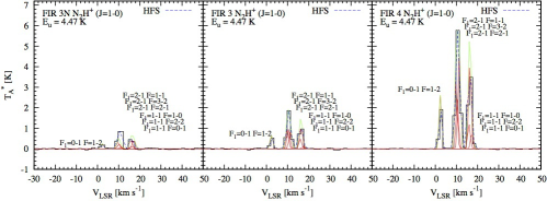
Figure A7: N₂H⁺ spectra. The HFS fitting result is shown by the blue dashed line.

As seen in Figs. A7 and A16, the HFS components of N₂H⁺ and NH₂D are blended due to the poor velocity resolution. To more accurately obtain the line parameters, we applied the HFS fitting to the N₂H⁺ and NH₂D spectra according to the document for Class/Gildas on the assumption that the all HFS components for each molecule have the same excitation temperature and velocity width, Gaussian line profiles as a function of velocity, and the multiple components do not overlap.

The opacity of the $i$th component, $\tau_{i}$($v$), is expressed as

$$\tau_{i}(v)=\tau_{i}^{\rm center}{\rm exp}\Biggl{(}-4{\rm ln}2\biggl{(}\frac{v-(V_{\rm sys}+\delta v_{i})}{dV_{\rm FWHM}}\biggr{)}^{2}\Biggr{)},$$ (A1)

where $\tau_{i}^{\rm center}$, $dV_{\rm FWHM}$, $\delta v_{i}$, and $V_{\rm sys}$ are the opacity at the line center of the $i$th component, the velocity width in FWHM, the velocity offset of the component $i$ with respect to the main component, and the systemic velocity of the target. The opacity of the all components, $\tau$ can be written as

$$\tau(v)=\tau_{\rm main}\Sigma^{N}_{i=1}r_{i}{\rm exp}\Biggl{(}-4{\rm ln}2\biggl{(}\frac{v-\delta v_{i}-V_{\rm sys}}{dV_{\rm FWHM}}\biggr{)}^{2}\Biggr{)},$$ (A2)

where $r_{i}$ is the relative strength of each component and $\Sigma^{N}_{i=1}r_{i}$=1 Thus, the antenna and excitation temperatures are related as

$$T_{\rm ant}(v)=\eta_{\rm mb}[T_{\rm ex}-T_{\rm bg}](1-e^{-\tau(v)})$$ (A3)

and the excitation temperature $T_{\rm ex}$ is derived as

$$T_{\rm ex}=T_{\rm bg}+\frac{T_{\rm ant}\tau_{\rm total}}{\tau_{\rm main}\eta_{\rm mb}},$$ (A4)

where $\tau_{\rm total}$ is $\tau_{\rm main}\Sigma^{N}_{i=1}r_{i}$.

Table A1 shows the HFS fitting results. The obtained line parameters of $V_{\rm sys}$ and $dV_{\rm FWHM}$ are consistent with those by the Gaussian fitting (see Sect 4.2) within the uncertainties. However, as shown in Figs. A7 and A16, there exist differences between the best-fit intensities in the Gaussian and HFS fitting. This is probably because the Gaussian fitting is affected by the blending of the HFS components.

Table A1: Results of HFS fitting

Molecule	Target	$T_{\rm ant}$ $\times$ $\tau$	$V_{\rm sys}$ [km/s]	$dV_{\rm FWHM}$ [km/s]	$\tau_{\rm main}$	$T_{\rm ex}$ [K]
N2H+ (1–0)	FIR 3N	2.4$\pm$0.4	11.10$\pm$0.04	1.72$\pm$0.16	0.82$\pm$0.5	16.4$\pm$15.3
N2H+ (1–0)	FIR 3	6.1$\pm$0.5	11.31$\pm$0.01	1.57$\pm$0.07	1.4$\pm$0.4	14.3$\pm$2.8
N2H+ (1–0)	FIR 4	23.0$\pm$0.3	11.37$\pm$0.01	1.49$\pm$0.01	2.4$\pm$0.1	26.4$\pm$0.5
NH2D (1–0)	FIR 4	1.4$\pm$0.2	10.90$\pm$0.14	1.58$\pm$0.15	1.5$\pm$0.6	6.1$\pm$4.9

A.2 Description of Each Line

A.2.1 CN

The CN emission is detected at the three positions of FIR 3N, 3, and 4, and their profiles are shown in Fig. A1. The CN emission is though to trace the ambient dense gas toward the regions.

A.2.2 CO and C¹⁷O

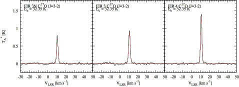
Figure A2: C¹⁷O spectra

Figure A2 shows a comparison among the C¹⁷O spectra at FIR 3N, 3, and 4. We note that the C¹⁷O (3–2) emission line has HFS, which is not resolved in our observations. Figure A20 shows the CO profiles at the three positions. The CO (3–2) spectra at the three positions consist of the two Gaussian components with the narrow and wide velocity widths. It is likely that the wide components of the CO (3–2) emission trace the molecular outflow. In fact, a previous study has detected the molecular outflow driven from FIR 3 in the CO (3–2) emission (Takahashi et al., 2008). On the other hand, the C¹⁷O spectra at the three positions have the single narrow (1.7–2.0 km s^-1) components, and are though to trace the ambient dense gas.

A.2.3 CS, C³⁴S, and ¹³CS

Figures A10, A21, and A24, show the ¹³CS, CS, and C³⁴S spectra at the three positions, respectively. The CS (2–1, 7–6) emission is detected at the three positions and have the narrow and wide components. Thus, we consider that the wide components trace the molecular outflow. In fact, NMA observations with a low-velocity resolution of 50 km s^-1 have revealed that the distribution of the CS (2–1) emission is similar to that of the CO (1–0, 3–2) molecular outflow (Shimajiri et al., 2008). The C³⁴S emission is detected at FIR 3 and 4, but the wide components are found only at FIR 4. This result suggests that the wide components trace the outflow shock. The ¹³CS emission is detected at FIR 3 and FIR 4 and has the only narrow component. As shown in Fig. A10, the emission-like feature with an S/N of 2.1 at FIR 3N can be marginally seen at the same LSR velocity as in FIR 3 and FIR 4. Thus, the non-detection of ¹³CS at FIR 3N is considered to be due to poor sensitivity. The velocity widths of the ¹³CS at FIR 3N and FIR 4 are 2.59 and 1.89 km s^-1, which are similar to those of the ambient dense-gas tracers having the only narrow component. Thus, the ¹³CS components likely trace the ambient dense gas.

Table 6 shows our estimated optical depths of the CS (2–1, 7–6) emission, assuming the same excitation temperature for the CS and C³⁴S lines and the [C³²S]/[C³⁴S] ratio of 22 (Wilson & Rood, 1994).

A.2.4 C₂H

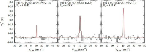
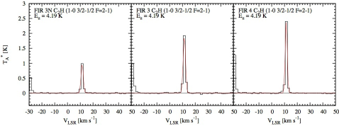
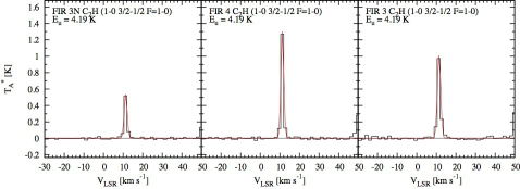
Figure A3: C₂H spectra

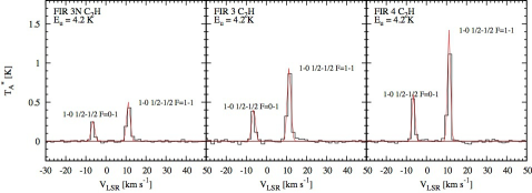
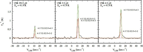
Figure A3: Continued.

Figure A3 shows a comparison of the C₂H lines among FIR 3N, FIR 3, and FIR 4. The C₂H emission is detected at the three positions and has the only narrow component. The velocity widths of C₂H (1–0 3/2–1/2 $F$=2–1) are 2.04, 2.17, and 1.84 km s^-1, which are similar to those in the typical dense-gas tracers such as the H¹³CO⁺ (1–0) line. These results suggest that the C₂H emission traces the ambient dense gas.

A.2.5 HCO⁺, H¹³CO⁺, and HC¹⁸O⁺

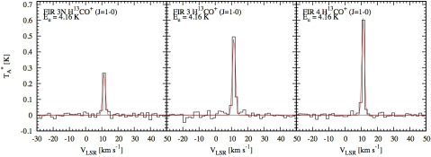
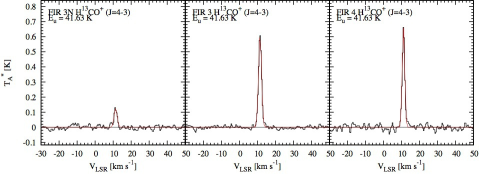
Figure A6: H¹³CO⁺ spectra

Figures A6, A19, and A23, show the H¹³CO⁺, HC¹⁸O⁺, and HCO⁺ lines, respectively. The HCO⁺ (1-0) emission is detected at FIR 3N, 3, and 4, and has the narrow and wide velocity components, suggesting that the emission traces the molecular outflow. Actually, previous mapping observations in the HCO⁺ (1–0) line have detected the molecular outflow driven by FIR 3 (Aso et al., 2000). The H¹³CO⁺ (1–0, 4–3) emission was also detected at the three positions. However, the H¹³CO⁺ emission has the single narrow velocity components with velocity widths of 1.6–1.8 km s^-1, suggesting that the emission traces the ambient dense gas. The HC¹⁸O⁺ emission is detected only at FIR 3 and has the only narrow component. As shown in Fig. A19, the emission-like feature with an S/N of 2.4 at FIR 4 can be marginally seen at the same LSR velocity as in FIR 3. Thus, the non-detection of the HC¹⁸O⁺ at FIR 4 is considered to be due to poor sensitivity. In Fig. 7(a), the 3$\sigma$ upper limit of HC¹⁸O⁺ at FIR 3N is plotted above the line of $N_{\rm mol}$ (FIR 3N)=$\frac{N_{\rm H^{13}CO^{+}}({\rm FIR\ 3N})}{N_{\rm H^{13}CO^{+}}({\rm FIR\ 4})}$$N_{\rm mol}$(FIR 4), suggesting the sensitivity for HC¹⁸O⁺ is poor. The velocity width of HC¹⁸O⁺ at FIR 3 is 1.02 km s^-1, which is similar to those of molecules having the only narrow component. Thus, the HC¹⁸O⁺ component likely traces the ambient dense gas.

We estimated the optical depth of the HCO⁺ (1–0) line, assuming the same excitation temperature for the HCO⁺ (1–0) and H¹³CO⁺ (1–0) lines and the [¹²C/¹³C] ratio of 62 (Langer & Penzias, 1993). Table 6 shows that the optical depth of the HCO⁺ (1–0) line toward FIR 3N, FIR 3, and FIR 4 is 9.7, 7.1, and 8.6, respectively, i.e., optically thick. Note that we could not cover the frequency of the HCO⁺ (4-3) line.

A.2.6 HNC, HN¹³C, H¹⁵NC, HCN, H¹³CN, and HC¹⁵N

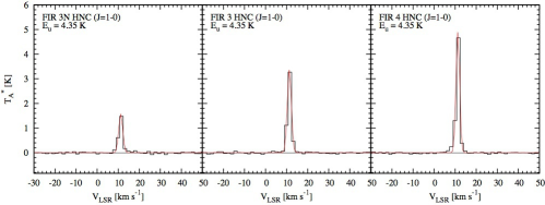
Figure A4: HNC spectra

Figures A4, A5, A18, A22, A27, and A28 show the HNC, HN¹³C, H¹⁵NC, HCN, H¹³CN, and HC¹⁵N spectra, respectively. The emission of HNC and HN¹³C are detected at the three positions. Their spectra consist of only narrow components with the velocity widths of $\sim$1 km s^-1, which are similar to those of the typical dense-gas tracers such as the H¹³CO⁺ (1–0) line. These results suggest that the emission of HNC and HN¹³C traces the ambient dense gas. In contrast, the spectra of HCN at the three positions have the narrow and wide velocity components, suggesting that the emission traces the molecular outflow. To analyze the hyper fine structure (HFS) of HCN, we assumed that the intensity ratio of the narrow to wide velocity components is the same for all the HFS components. The wide components of the H¹³CN (1–0, 4–3) and HC¹⁵N emission are detected only at FIR 4, suggesting that the wide components trace the outflow shock.

The H¹⁵NC emission is detected at FIR 3N and FIR 4 and have the only narrow component. The 3$\sigma$ upper limit of H¹⁵NC at FIR 3 is plotted below the line of $N_{\rm mol}$(FIR 3)=$\frac{N_{\rm H^{13}CO^{+}}({\rm FIR\ 3})}{N_{\rm H^{13}CO^{+}}({\rm FIR\ 4})}$$N_{\rm mol}$(FIR 4) in Fig. 7(b). Thus, we cannot conclude that the non-detection of H¹⁵NC at FIR 3 is due to poor sensitivity. The velocity width of H¹⁵NC at FIR 4 is 1.82 km s^-1, which is similar to those of molecules having the only narrow component. Thus, the H¹⁵NC component likely traces the ambient dense gas.

We estimated the optical depths of the HNC emission, assuming the same excitation temperature for the HNC and HN¹³C lines and the [¹²C]/[¹³C] ratio of 62 (Langer & Penzias, 1993). The optical depth of the HNC (1–0) line with a transition of 1–0 is estimated to be 3.1, 4.5, and 6.2 toward FIR 3N, FIR 3, and FIR 4, respectively, i.e., optically thick. Similarly, we estimated the optical depths of the HCN (1–0, 4–3) emission, assuming the same excitation temperature for the HCN and H¹³CN lines. The HCN emission is shown to be optically thick. Particularly, the optical depths of the wide components of the HCN (1–0) lines are too high ($>$ 10) compared with those of the narrow components. This is probably due to our assumption that the intensity ratio of the narrow to wide velocity components is the same for all the HFS transitions.

A.2.7 N₂H⁺

Figure A7 shows a comparison of the N₂H⁺ spectra among FIR 3N, FIR 3, and FIR 4. The N₂H⁺ emission is detected at the three positions and has the only narrow component, suggesting that the emission traces the ambient dense gas.

A.2.8 c-C₃H₂

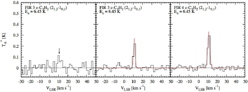
Figure A8: c-C₃H₂ spectra. The vertical arrow in the left panel shows the detection, but the peak is not fitted well by the single Gaussian component due to insufficient velocity resolution.

Figure A8 shows a comparison of the c-C₃H₂ lines among FIR 3N, FIR 3, and FIR 4. The c-C₃H₂ (2–1) emission with the single narrow component is detected at the three positions. The velocity width and total integrated intensity at FIR 3 are similar to those at FIR 4. These results suggest that the c-C₃H₂ emission traces the ambient dense gas.

A.2.9 NH₂D

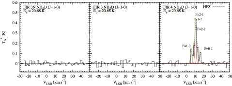
Figure A16: NH₂D spectra. The HFS fitting result is shown by the blue dashed line.

Figure A16 shows the NH₂D spectra at FIR 3N, FIR 3, and FIR 4. The NH₂D emission is detected only at FIR 4. The velocity width is 1.5 km s^-1 which is similar to those of the typical dense-gas tracers. Thus, the NH₂D emission traces the dense gas. In Fig. 7, the 3$\sigma$ upper limits of NH₂D at FIR 3N and FIR 3 are plotted below the lines of $N_{\rm mol}$(FIR 3N)=$\frac{N_{\rm H^{13}CO^{+}}({\rm FIR\ 3N})}{N_{\rm H^{13}CO^{+}}({\rm FIR\ 4})}$ and $N_{\rm mol}$(FIR 4) and $N_{\rm mol}$(FIR 3)=$\frac{N_{\rm H^{13}CO^{+}}({\rm FIR\ 3})}{N_{\rm H^{13}CO^{+}}({\rm FIR\ 4})}$$N_{\rm mol}$(FIR 4), suggesting that the sensitivities in NH₂D seem sufficient in FIR 3N and FIR 3, and the fractional abundance of NH₂D in FIR 4 is likely higher than those in FIR 3N and FIR 3.

A.2.10 SiO

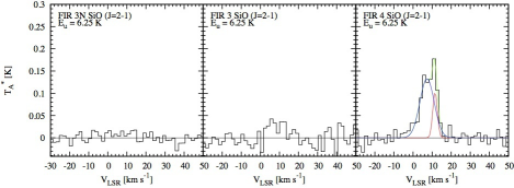
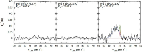
Figure A26: SiO spectra

Figure A26 shows the SiO (2–1, 8–7) spectra at FIR 3N, 3, and 4. The SiO emission is detected only at FIR 4 and has the narrow and wide components. The velocity widths of the wide components are 8–10 km s^-1, which are extremely larger than those of the H¹³CO⁺ narrow components (1.6–2.1 km s^-1). The peak velocities of the narrow and wide components are 11 and 5 km s^-1, which is consistent with the NMA observations (see Fig 8(c) in Shimajiri et al., 2008). The NMA observations in SiO revealed that the SiO emission is distributed at the interface between the outflow driven from FIR 3 and the FIR 4 clump. These facts suggest that the SiO emission traces the outflow shock.

A.2.11 SO

Figure A25 shows a comparison of the SO lines among FIR 3N, FIR 3, and FIR 4. We have succeeded in detecting the four transitions of SO. At FIR 4, all the transitions have the wide velocity components, and the peak velocities of the wide components are blueshifted with respect to those of the narrow components. The difference in peak velocity between the narrow and wide components is quite similar to that of the SiO emission at FIR 4, suggesting that the wide components of the SO emission trace the outflow shock. However, the wide components of the SO emission with higher upper energy levels are also seen at FIR 3. Thus, there are two possibilities. First is that the SO emission traces the molecular outflow and the non-detection at FIR 3N and FIR 3 of the wide components is due to poor sensitivity. Second is that the SO emission traces the outflow shock and the wide components at FIR 3 trace the outflow shock near the driving source where the outflow gas is being launched. The possible reason for the wide components of only SO being detected at FIR 3 is that the SO emission have higher upper energy levels ($E_{\rm u}$ $>$ 80 K) and traces the warm region.

A.2.12 H₂CS

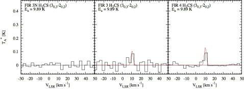
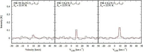
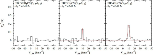
Figure A30: H₂CS spectra

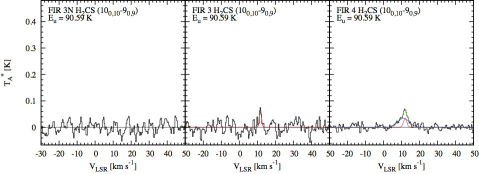
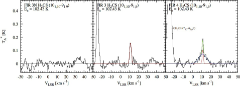
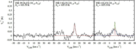
Figure A30: Continued.

Figure A30 shows a comparison of the H₂CS lines among FIR 3N, FIR 3, and FIR4. The H₂CS emission is detected at the three positions. The H₂CS emission with an upper-state energy of $>$ 90 K has the narrow and wide components. According to our criteria of the line identification (see Sect. 4.2), the H₂CS (3_0,3–2_0,2, 3_1,3–2_1,2, 3_1,2–2_1,1) lines with a upper-state energy of $<$ 90 K are identified as spectra having a single Gaussian component. The wide components of the H₂CS emission are detected only at FIR 4, suggesting that these components trace the outflow shock.

A.2.13 HC₃N

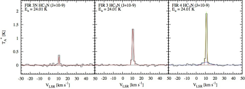
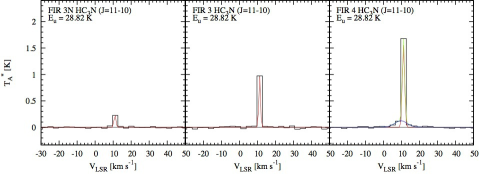
Figure A31: HC₃N spectra

Figure A31 shows a comparison of the HC₃N (10–9, 11–10) lines among FIR 3N, FIR 3, and FIR 4. The two transitions are detected at the three positions. Only at FIR 4, the HC₃N emission has the wide velocity component, suggesting that the wide components trace the outflow shock. Owing to a slight difference between the two upper energy levels of the transitions, we could not derive the rotation temperature and column density of HC₃N from the rotation diagram.

A.2.14 CH₃OH

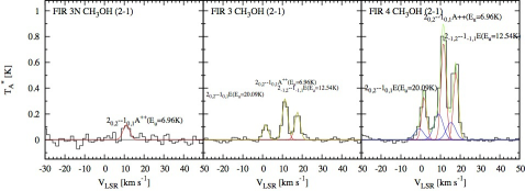
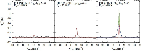
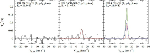
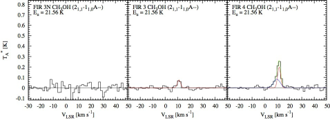
Figure A32: CH₃OH spectra

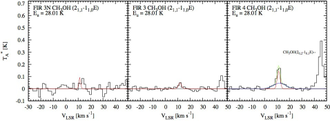
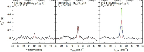
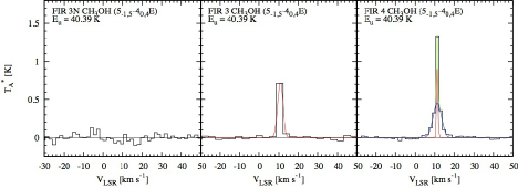
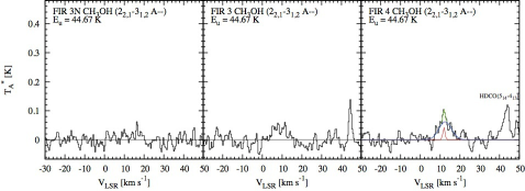
Figure A32: Continued.

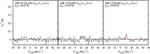
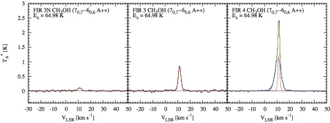
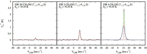
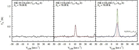
Figure A32: Continued.

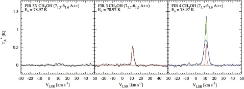
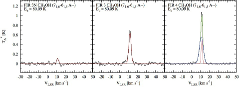
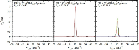
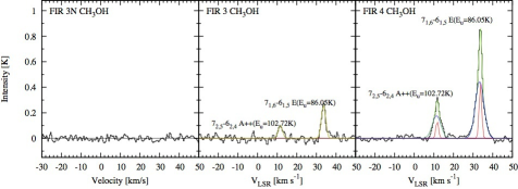
Figure A32: Continued.

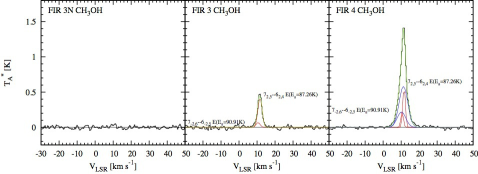
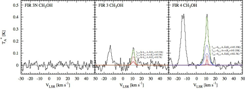
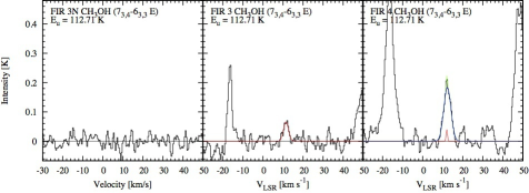
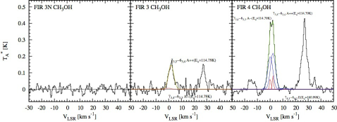
Figure A32: Continued.

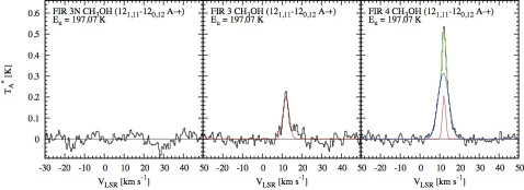
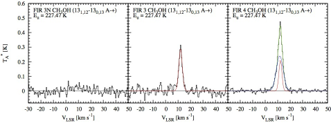
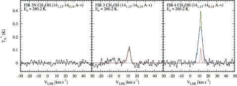
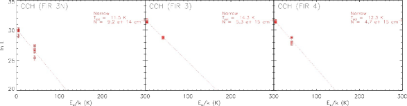
Figure A32: Continued.

Figure A32 shows a comparison among the spectra of the CH₃OH lines at FIR 3N, FIR 3, and FIR 4. The wide components of the CH₃OH lines are detected only at FIR 4, suggesting that the wide components trace the outflow shock. In addition, the intensity ratio of the wide to narrow components of the CH₃OH line tends to increase with increasing upper state energy level in the transition. This result suggests that the wide component of the CH₃OH line traces the high temperature part of the outflow-shocked region at FIR 4. In fact, the rotation diagram analysis has revealed that the rotation temperatures of the CH₃OH wide components are as high as 46.4$\pm$6.8 K for CH₃OH A and 25.4$\pm$3.3 K for CH₃OH E.

A.2.15 HCS⁺

Figure A15 shows the HCS⁺ spectra at FIR 3N, FIR 3, and FIR 4. The HCS⁺ emission is detected only at FIR 4. The intensity and velocity width are 0.07 K in $T_{\rm A}^{*}$ (corresponding to a signal-to-noise ratio of 3.5) and 3.0 km s^-1. The velocity width is twice as large more than twice as large as those of the ambient dense-gas tracers. It is possible that the HCS⁺ emission has a wide component only at FIR 4 and traces the outflow shock. The reason for the non-detection of the wide component is considered to be due to poor sensitivity. In fact, the signal-to-noise ratio of the emission at FIR 4 is too low to separate the two components. We cannot, however, exclude another possibility that the non-detection of the emission at FIR 3 and FIR 3N is due to poor sensitivity (see the center panel of Fig. A15) and that the emission tracers the outflow. To reveal whether the emission has the wide component or not, higher sensitivity observations are required.

A.2.16 H₂CO, H${}_{2}^{13}$CO, and HDCO

Figures A17, A29, and A11 show the H₂CO, H${}_{2}^{13}$CO, and HDCO spectra, respectively. The H₂CO emission is detected only at FIR 4. The velocity width of the H₂CO emission is 3.8 km s^-1 which is twice as large more than twice as large as the typical width of the ambient dense-gas tracers. Considering the weak intensity of the emission, there remains a possibility that the wide component of H₂CO is not detected due to poor sensitivity. Thus, we classify this molecule as a possible shock tracer.

The H${}_{2}^{13}$CO emission is detected at the three positions. The wide component is, however, seen only at FIR 4. This result suggests that the wide component of the H${}_{2}^{13}$CO emission traces the outflow shock.

The HDCO emission is detected at FIR 3 and FIR 4. The velocity widths at FIR 3 and FIR 4 are 2.9 km s^-1 and 3.5 km s^-1, respectively. These values are twice as large more than twice as large as the typical velocity width of the ambient dense-gas tracers, and the HDCO emission possibly traces the outflow or the outflow shock.

A.2.17 HNCO

Figure A12 shows the HNCO spectra at FIR 3N, FIR 3, and FIR 4. The HNCO emission is detected at FIR 3 and FIR 4. At FIR 3N, a emission-like feature with an S/N of 2.0 is seen, and thus, the non-detection at FIR 3N might be due to poor sensitivity. The intensity and velocity width at FIR 3 are 0.114 K in $T_{\rm A}^{*}$ (S/N=6.1) and 1.48 km s^-1, respectively, and 0.083 K (S/N=6.1) and 3.15 km s^-1 at FIR 4. The velocity width at FIR 4 is twice as large more than twice as large as that at FIR 3 and those of the ambient dense-gas tracers. We speculate that the emission has a wide component only at FIR 4 and traces the outflow shock. The reason for the non-detection of the wide component would be due to poor sensitivity. In fact, the signal-to-noise ratio of the emission is too low to separate the two components. We cannot, however, exclude another possibility that the non-detection of the wide component at FIR 3 and FIR 3N is due to poor sensitivity. To reveal whether the emission has the wide component or not, higher sensitivity observations are required.

A.2.18 CH₃CN

Figure A9 shows a comparison of the CH₃CN lines among FIR 3N, FIR 3, and FIR 4. The CH₃CN emission are detected at the three positions and have the single narrow components. These results suggest that the CH₃CN emission traces the ambient dense gas.

A.2.19 CH₃CCH

Figure A13 shows a comparison of the CH₃CCH lines among FIR 3N, FIR 3, and FIR 4. The CH₃CCH emission is detected at FIR 3 and FIR 4 and has the single narrow components. At FIR 3N, emission-like features of CH₃CCH (6₁-5₁) with an S/N of 2.2 are marginally seen at the same velocities as in FIR 3 and FIR 4. Thus, the non-detection of CH₃CCH at FIR 3N is considered to be due to poor sensitivity. These results suggest that the CH₃CCH emission traces the ambient dense gas. However, the rotation temperatures of the CH₃CCH transitions at FIR 4 are estimated to be 32.5$\pm$3.8 K for ortho and 53.2$\pm$36.4 K for para, which are twice as large more than twice as large as the mean temperature of the dense-gas tracers of C₂H and H¹³CO⁺ (12.5$\pm$1.4 K) . We cannot exclude a possibility that the CH₃CCH traces the outflow and/or outflow shock.

A.2.20 CH₃CHO

Figure A14 shows a comparison of the CH₃CHO lines among FIR 3N, FIR 3, and FIR 4. The CH₃CHO lines are detected only at FIR 4 except the CH₃CHO (5_1,5–4_1,4A) transition. The velocity widths of the CH₃CHO lines at FIR 4 are 2–4 km s^-1, which twice as large more than twice as large as the mean velocity width of the ambient dense-gas tracers and the velocity width at FIR 3 (2.38 km s^-1). Thus, we consider the CH₃CHO emission as possible shock tracers.

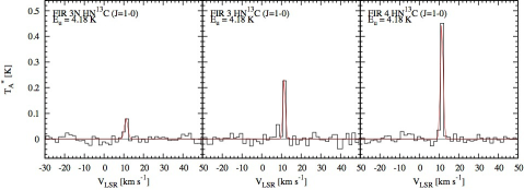
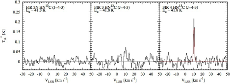
Figure A5: HN¹³C spectra

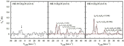
Figure A9: CH₃CN spectra. The vertical arrow in the left panel shows the detection, but the peak is not fitted well by the single Gaussian component due to insufficient velocity resolution.

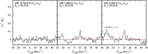
Figure A11: HDCO spectra

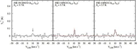
Figure A12: HNCO spectra. The vertical arrow in the right panel shows the emission-like feature.

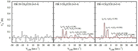
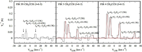
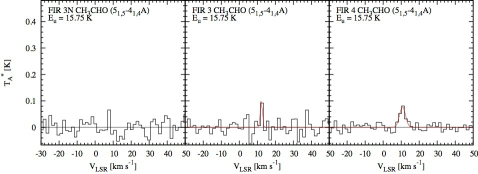
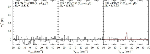
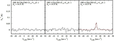
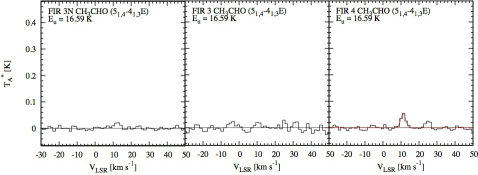
Figure A13: CH₃CCH spectra. The vertical arrow in the right panel shows the emission-like feature.

Figure A14: CH₃CHO spectra

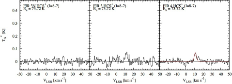
Figure A15: HCS⁺ spectra

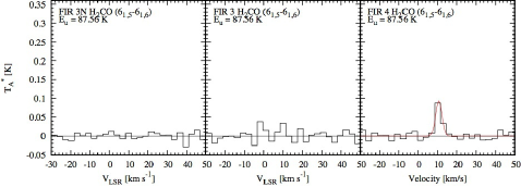
Figure A17: H₂CO spectra

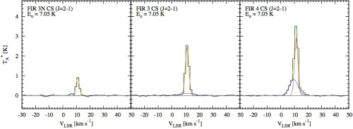
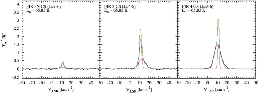
Figure A21: CS spectra

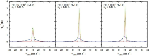
Figure A23: HCO⁺ spectra

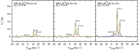
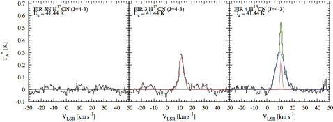
Figure A27: H¹³CN spectra

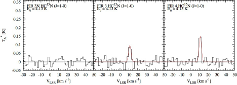
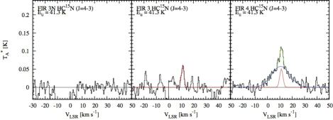
Figure A28: HC¹⁵N spectra

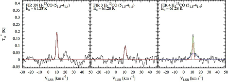
Figure A29: H${}_{2}^{13}$CO spectra

Figure A33: C₂H rotation diagrams. The left, center, and right panels are for FIR 3N, FIR 3, and FIR 4, respectively. The error bars correspond to the 1$\sigma$ uncertainties.

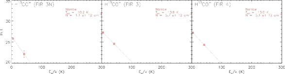
Figure A34: H¹³CO⁺ Rotation Diagrams.

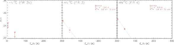
Figure A35: HN¹³C Rotation Diagrams. The downward arrow in the left panel means the 3$\sigma$ upper limit.

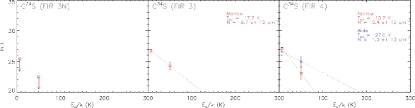
Figure A36: C³⁴S Rotation Diagrams.

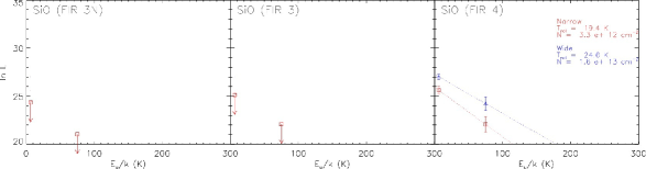
Figure A37: SiO Rotation Diagrams.

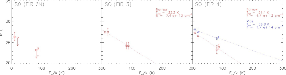
Figure A38: SO Rotation Diagrams.

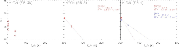
Figure A39: H¹³CN Rotation Diagrams.

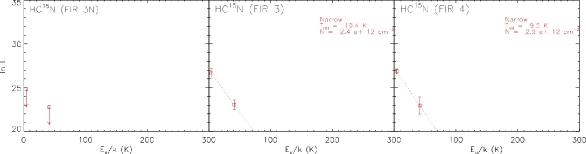
Figure A40: HC¹⁵N Rotation Diagrams.

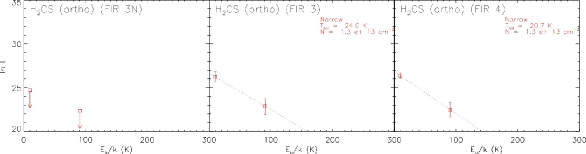
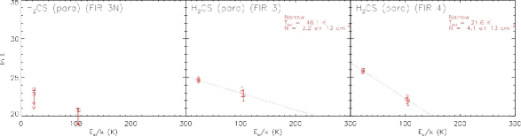
Figure A41: H₂CS Rotation Diagrams.

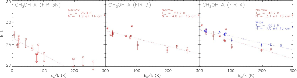
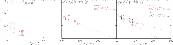
Figure A42: CH₃OH Rotation Diagrams.

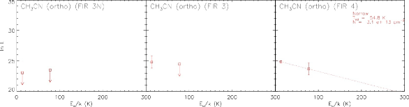
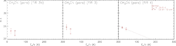
Figure A43: CH₃CN Rotation Diagrams.

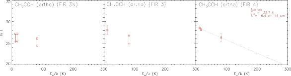
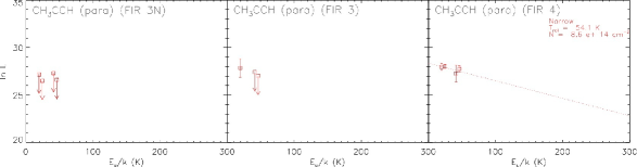
Figure A44: CH₃CCH Rotation Diagrams.

Table A2: Parameters of the Molecular Lines Detected in FIR 3N

		$Narrow\ Component$			$Wide\ Component$
Molecule with Transition	Rest Freq.	$V_{\rm sys}$	$T_{\rm peak}$	$dV_{\rm FWHM}$	$V_{\rm sys}$	$T_{\rm peak}$	$dV_{\rm FWHM}$
	[GHz]	[km s-1]	[K]	[km s-1]	[km s-1]	[K]	[km s-1]
c-C3H2 (21,2–10,1)	85.338906	$\cdots$	0.123d	$\cdots$	$\cdots$
H13CN ($J$=1–0 $F$=1–1)	86.3387367	11.1	0.103	1.69	$\cdots$
H13CN ($J$=1–0 $F$=2–1)	86.3401764	11.1	0.137	1.69	$\cdots$
H13CN ($J$=1–0 $F$=0–1)	86.3422551	11.1	0.027	1.69	$\cdots$
H13CO+ ($J$=1-0)	86.754288	11.4	0.267	1.98	$\cdots$
HN13C ($J$=1–0)	87.090859	11.2	0.080a	2.01	$\cdots$
C2H (1–0 3/2–1/2 $F$=1–1)	87.284156	11.1	0.161	0.55	$\cdots$
C2H (1–0 3/2–1/2 $F$=2–1)	87.316925	11.5	0.987	2.04	$\cdots$
C2H (1–0 3/2–1/2 $F$=1–0)	87.328624	11.3	0.541	1.80	$\cdots$
C2H (1–0 1/2–1/2 $F$=1–1)	87.402004	11.2	0.500	2.09	$\cdots$
C2H (1–0 1/2–1/2 $F$=0–1)	87.407165	11.2	0.256	2.09	$\cdots$
HCN ($J$=1–0 $F$=1-1)	88.6304157	11.0	0.754	2.60	11.1	0.041a,c	13.62
HCN ($J$=1–0 $F$=2-1)	88.6318473	11.0	1.833	2.60	11.1	0.100a	13.62
HCN ($J$=1–0 $F$=0-1)	88.633936	11.0	0.350	2.60	11.1	0.019a,c	13.62
H15NC ($J$=1-0)	88.865692	$\cdots$	0.055d	$\cdots$	$\cdots$
HCO+ ($J$=1–0)	89.188526	11.1	1.838	2.69	9.3	0.392	20.19
HNC ($J$=1–0)	90.663564	11.2	1.573	2.25	$\cdots$
HC3N ($J$=10–9)	90.978989	11.3	0.381	0.54	$\cdots$
CH3CN (JK=51–41)	91.985313	$\cdots$	0.082d	$\cdots$	$\cdots$
N2H+ (1–0 $F_{1}$=1–1 $F$=0–1)	93.171621	10.8	0.408	2.20	$\cdots$
N2H+ (1–0 $F_{1}$=1–1 $F$=2–2)	93.171917	10.8	0.110	2.20	$\cdots$
N2H+ (1–0 $F_{1}$=1–1 $F$=1–0)	93.172053	10.8	0.075	2.20	$\cdots$
N2H+ (1–0 $F_{1}$=2–1 $F$=2–1)	93.17348	10.8	0.416	2.20	$\cdots$
N2H+ (1–0 $F_{1}$=2–1 $F$=3–2)	93.173777	10.8	0.216	2.20	$\cdots$
N2H+ (1–0 $F_{1}$=2–1 $F$=1–1)	93.173967	10.8	0.312	2.20	$\cdots$
N2H+ (1–0 $F_{1}$=0–1 $F$=1–2)	93.176265	10.8	0.240	2.20	$\cdots$
CH3OH (20,2–10,1A++)	96.741377	11.1	0.117	3.97	$\cdots$
CH3OH (21,1–11,0E)	96.755507	11.4	0.097	1.44	$\cdots$
CS ($J$=2–1)	97.980953	11.7	0.744	0.89	10.9	0.673	3.31
SO ($N,J$=2,3-1,2)	99.299905	10.9	0.154	3.20	$\cdots$
HC3N ($J$=11–10)	100.076386	11.0	0.235	1.28	$\cdots$
H2CS (31,3–21,2)	101.477885	10.5	0.043	3.28	$\cdots$
C17O ($J$=3–2)	337.060974	10.8	0.781	1.88	$\cdots$
CH3OH (7-1,7–6-1,6 E)	338.344605	11.5	0.140	2.63	$\cdots$
CH3OH (70,7–60,6 A++)	338.408718	11.2	0.103	3.52	$\cdots$
CN (3–2 $J$=5/2–3/2 $F$=5/2–5/2)	340.008097	11.3	0.023	2.48	$\cdots$
CN (3–2 $J$=5/2–3/2 $F$=7/2–5/2)	340.031567	11.3	0.374	2.48	$\cdots$
CN (3–2 $J$=5/2–3/2 $F$=5/2–3/2)	340.035525	11.3	0.286	2.48	$\cdots$
CN (3–2 $J$=7/2–5/2 $F$=7/2–5/2)	340.247625	11.1	1.020	2.48b	$\cdots$
CN (3–2 $J$=7/2–7/2 $F$=5/2–5/2)	340.261818	11.1	0.039	2.48b	$\cdots$
CN (3–2 $J$=7/2–7/2 $F$=7/2–7/2)	340.265025	11.1	0.089	2.48b	$\cdots$
CH3OH (71,6–61,5 A–)	341.415641	11.3	0.108	2.50	$\cdots$
CS ($J$=7–6)	342.882843	11.6	0.351	2.86	11.8	0.078	11.08
H${}_{2}^{13}$CO (51,5–41,4)	343.325714	10.7	0.196	2.36	$\cdots$
CO ($J$=3–2)	345.79599	11.7	13.9	5.61	9.2	7.400	12.22
H13CO+ ($J$=4–3)	346.998352	11.4	0.126	2.00	$\cdots$
C2H (4–3 9/2–7/2 $F$=5–4)	349.337741	11.8	0.135	2.22	$\cdots$
C2H (4–3 9/2–7/2 $F$=4–3)	349.339067	11.8	0.859	2.22	$\cdots$
C2H (4–3 7/2–5/2 $F$=4–3)	349.399342	11.1	0.516	2.02	$\cdots$
C2H (4–3 7/2–5/2 $F$=3–2)	349.400692	11.1	0.249	2.02	$\cdots$
CH3OH (40,4–3-1,3 E)	350.687651	11.0	0.103	2.37	$\cdots$
CH3OH (11,1–00,0 A++)	350.90507	11.1	0.098	2.07	$\cdots$
HCN ($J$=4–3)	354.505493	11.6	0.742	2.96	10.2	0.280	10.49

Table A3: Parameters of the Molecular Lines Detected in FIR 3

		$Narrow\ Component$			$Wide\ Component$
Molecule with Transition	Rest Freq.	$V_{\rm sys}$	$T_{\rm peak}$	$dV_{\rm FWHM}$	$V_{\rm sys}$	$T_{\rm peak}$	$dV_{\rm FWHM}$
	[GHz]	[km s-1]	[K]	[km s-1]	[km s-1]	[K]	[km s-1]
CH3OH (5-1,5–40,4E)	84.521206	10.8	0.744	3.13	$\cdots$
c-C3H2 (21,2–10,1)	85.338906	11.2	0.274	2.03	$\cdots$
CH3CCH (JK=53–43)	85.4426	11.2	0.050b,e	2.02	$\cdots$
CH3CCH (JK=52–42)	85.450765	11.2	0.050b,e	2.02	$\cdots$
CH3CCH (JK=51–41)	85.455665	11.2	0.110b	2.02	$\cdots$
CH3CCH (JK=50–40)	85.457299	11.2	0.140b	2.02	$\cdots$
HC15N ($J$=1–0)	86.054967	11.2	0.098	3.26	$\cdots$
SO ($N,J$=2,2–1,1)	86.093983	10.1	0.065	4.78	$\cdots$
H13CN ($J$=1–0 $F$=1–1)	86.3387367	11.3	0.236	2.22	$\cdots$
H13CN ($J$=1–0 $F$=2–1)	86.3401764	11.3	0.358	2.22	$\cdots$
H13CN ($J$=1–0 $F$=0–1)	86.3422551	11.3	0.052e	2.22	$\cdots$
H13CO+ ($J$=1-0)	86.754288	11.5	0.502	2.16	$\cdots$
HN13C ($J$=1–0)	87.090859	11.4	0.240	1.43	$\cdots$
C2H (1–0 3/2–1/2 $F$=1–1)	87.284156	11.3	0.247	2.45	$\cdots$
C2H (1–0 3/2–1/2 $F$=2–1)	87.316925	11.5	1.924	2.17	$\cdots$
C2H (1–0 3/2–1/2 $F$=1–0)	87.328624	11.4	1.031	1.95	$\cdots$
C2H (1–0 1/2–1/2 $F$=1–1)	87.402004	11.3	0.943	2.17	$\cdots$
C2H (1–0 1/2–1/2 $F$=0–1)	87.407165	11.3	0.410	2.17	$\cdots$
HNCO (40,4-30,3)	87.925238	11.6	0.114	1.48	$\cdots$
HCN ($J$=1–0 $F$=1-1)	88.6304157	11.5	1.847	2.77	10.2	0.043b,c	15.32
HCN ($J$=1–0 $F$=2-1)	88.6318473	11.5	4.285	2.77	10.2	0.100b	15.32
HCN ($J$=1–0 $F$=0-1)	88.633936	11.5	0.844	2.77	10.2	0.0197b,c	15.32
HCO+ ($J$=1–0)	89.188526	11.6	4.631	2.22	10.9	0.499	10.67
HNC ($J$=1–0)	90.663564	11.3	3.372	2.24	$\cdots$
HC3N ($J$=10–9)	90.978989	11.2	1.331	1.90	$\cdots$
CH3CN (JK=53–43)	91.971465	11.0	0.063e	2.85	$\cdots$
CH3CN (JK=52–42)	91.979994	11.0	0.084	2.85	$\cdots$
CH3CN (JK=51–41)	91.985313	11.0	0.150	2.85	$\cdots$
CH3CN (JK=50–40)	91.987086	11.0	0.182	2.85	$\cdots$
13CS ($J$=2–1)	92.49427	10.9	0.118	2.59	$\cdots$
N2H+ (1–0 $F_{1}$=1–1 $F$=0–1)	93.171621	11.4	0.088	1.64	$\cdots$
N2H+ (1–0 $F_{1}$=1–1 $F$=2–2)	93.171917	11.4	1.060	1.64	$\cdots$
N2H+ (1–0 $F_{1}$=1–1 $F$=1–0)	93.172053	11.4	0.490	1.64	$\cdots$
N2H+ (1–0 $F_{1}$=2–1 $F$=2–1)	93.17348	11.4	0.818	1.64	$\cdots$
N2H+ (1–0 $F_{1}$=2–1 $F$=3–2)	93.173777	11.4	0.952	1.64	$\cdots$
N2H+ (1–0 $F_{1}$=2–1 $F$=1–1)	93.173967	11.4	0.931	1.64	$\cdots$
N2H+ (1–0 $F_{1}$=0–1 $F$=1–2)	93.176265	11.4	0.644	1.64	$\cdots$
CH3CHO (51,5-41,4A)	93.580914	12.3	0.111	1.26	$\cdots$
CH3OH (80,8–71,7A++)	95.169516	11.0	3.038	2.39	$\cdots$
CH3OH (21,2–11,1A++)	95.91431	10.3	0.062	4.25	$\cdots$
C34S ($J$=2–1)	96.41295	11.1	0.180	2.21	$\cdots$
CH3OH (2-1,2–1-1,1E)	96.739363	11.3	0.215	3.21	$\cdots$
CH3OH (20,2–10,1A++)	96.741377	11.3	0.321	3.21	$\cdots$
CH3OH (20,2–10,1E)	96.744549	11.3	0.118	3.21	$\cdots$
CH3OH (21,1–11,0A–)	97.582808	11.1	0.076	2.99	$\cdots$
CS ($J$=2–1)	97.980953	11.2	2.460	3.01	11.6	0.101	10.99
SO ($N,J$=2,3-1,2)	99.299905	11.2	0.264	2.79	$\cdots$
HC3N ($J$=11–10)	100.076386	11.1	0.973	1.08	$\cdots$
H2CS (31,3–21,2)	101.477885	9.7	0.100b	1.60	$\cdots$
CH3CCH (JK=63–53)	102.530346	10.6	0.025b,e	3.14	$\cdots$
CH3CCH (JK=62–52)	102.540143	10.6	0.070b	3.14	$\cdots$
CH3CCH (JK=61–51)	102.546023	10.6	0.110b	3.14	$\cdots$
CH3CCH (JK=60–50)	102.547983	10.6	0.140b	3.14	$\cdots$
H2CS (30,3–20,2)	103.040548	10.8	0.108	2.62	$\cdots$
H2CS (31,2–21,1)	104.617109	10.5	0.155	0.95	$\cdots$
HDCO (514–413)	335.096771	11.1	0.100	2.93	$\cdots$
CH3OH (71,7–61,6 A++)	335.582022	11.7	0.505	2.69	$\cdots$
CH3OH (121,11–120,12 A-+)	336.865153	12.0	0.202	3.65	$\cdots$
C17O ($J$=3–2)	337.060974	11.1	0.898	2.10	$\cdots$
C34S ($J$=7–6)	337.396454	11.3	0.150	2.47	$\cdots$
H2CS (101,10–91,9)	338.083191	11.5	0.164	2.17	$\cdots$
CH3OH (70,7–60,6 E)	338.124498	11.5	0.560	2.57	$\cdots$
CH3OH (7-1,7–6-1,6 E)	338.344605	11.6	0.746	2.66	$\cdots$
CH3OH (70,7–60,6 A++)	338.408718	11.6	0.843	2.56	$\cdots$
CH3OH (74,4–64,3 A–)a	338.512627	11.6	0.072	3.60	$\cdots$
CH3OH (74,3–64,2 A++)a	338.512639	11.6	0.033	3.60	$\cdots$
CH3OH (73,5–63,4 A++)a	338.540824	11.3	0.146	4.88	$\cdots$
CH3OH (73,4–63,3 E)	338.583223	11.6	0.068	2.85	$\cdots$
CH3OH (71,6–61,5 E)	338.614953	11.7	0.264	2.52	$\cdots$
CH3OH (72,5–62,4 A++)	338.639807	11.7	0.102	2.52	$\cdots$
CH3OH (72,5–62,4 E)a	338.721694	11.6	0.418	2.70	$\cdots$
CH3OH (7-2,6–6-2,5 E)a	338.722914	11.6	0.067	2.70	$\cdots$
CN (3–2 $J$=5/2–5/2 $F$=7/2–7/2)	339.51669	11.5	0.131	1.96	$\cdots$
CN (3–2 $J$=5/2–3/2 $F$=5/2–5/2)	340.008097	11.6	0.149	2.53	$\cdots$
CN (3–2 $J$=5/2–3/2 $F$=3/2–3/2)	340.019605	11.6	0.108	2.53	$\cdots$
CN (3–2 $J$=5/2–3/2 $F$=7/2–5/2)	340.031567	11.6	1.064	2.53	$\cdots$
CN (3–2 $J$=5/2–3/2 $F$=5/2–3/2)	340.035525	11.6	0.834	2.53	$\cdots$
CN (3–2 $J$=7/2–5/2 $F$=7/2–5/2)	340.247625	11.3	2.488	2.53d	$\cdots$
CN (3–2 $J$=7/2–7/2 $F$=5/2–5/2)	340.261818	11.3	0.165	2.53d	$\cdots$
CN (3–2 $J$=7/2–7/2 $F$=7/2–7/2)	340.265025	11.3	0.205	2.53d	$\cdots$
HC18O+ ($J$=4–3)	340.630707	11.3	0.074	2.16d	$\cdots$
SO ($N,J$=8,7–7,6)	340.71435	11.3	0.124	1.90	8.3	0.054e	10.81
CH3OH (71,6–61,5 A–)	341.415641	11.7	0.656	3.10	$\cdots$
CH3OH (131,12–130,13 A-+)	342.729781	12.0	0.288	3.33	$\cdots$
CS ($J$=7–6)	342.882843	11.5	1.899	2.59	12.9	0.563	9.09
H2CS (100,10–90,9)	342.94646	11.7	0.074	1.29	$\cdots$
H${}_{2}^{13}$CO (51,5–41,4)	343.325714	11.6	0.099	2.64	$\cdots$
H13CN ($J$=4–3)	345.339752	11.9	0.264	4.64	$\cdots$
CO ($J$=3–2)	345.79599	11.4	16.419	5.50	12.3	4.727	12.56
SO ($N,J$=8,9–7,8)	346.528587	11.2	0.129	2.07	11.2	0.058e	10.16
H13CO+ ($J$=4–3)	346.998352	11.4	0.615	1.97	$\cdots$
H2CS (101,9–91,8)	348.534363	11.4	0.133	3.73	$\cdots$
CH3OH (141,13–140,14 A-+)	349.106954	11.7	0.114	3.81	$\cdots$
C2H (4–3 9/2–7/2 $F$=5–4)	349.337741	11.4	1.910	2.27	$\cdots$
C2H (4–3 9/2–7/2 $F$=4–3)	349.339067	11.4	1.367	2.27	$\cdots$
C2H (4–3 7/2–5/2 $F$=4–3)	349.399342	11.6	1.132	2.28	$\cdots$
C2H (4–3 7/2–5/2 $F$=3–2)	349.400692	11.6	1.145	2.28	$\cdots$
CH3OH (40,4–3-1,3 E)	350.687651	11.3	0.320	2.86	$\cdots$
CH3OH (11,1–00,0 A++)	350.90507	11.5	0.376	2.72	$\cdots$
HCN ($J$=4–3)	354.505493	12.0	2.890	3.08	12.1	1.151	8.37

Table A4: Parameters of the Molecular Lines Detected in FIR 4

		$Narrow\ Component$			$Wide\ Component$
Molecule with Transition	Rest Freq.	$V_{\rm sys}$	$T_{\rm peak}$	$dV_{\rm FWHM}$	$V_{\rm sys}$	$T_{\rm peak}$	$dV_{\rm FWHM}$
	[GHz]	[km s-1]	[K]	[km s-1]	[km s-1]	[K]	[km s-1]
CH3OH (5-1,5–40,4E)	84.521206	11.3	0.950	0.72	11.3	0.451	4.93
c-C3H2 (21,2–10,1)	85.338906	11.2	0.333	2.59	$\cdots$
CH3CCH (JK=53–43)	85.4426	11.1	0.040b,e	1.98	$\cdots$
CH3CCH (JK=52–42)	85.450765	11.1	0.060b	1.98	$\cdots$
CH3CCH (JK=51–41)	85.455665	11.1	0.140b	1.98	$\cdots$
CH3CCH (JK=50–40)	85.457299	11.1	0.260b	1.98	$\cdots$
NH2D (1(1,1)0+ -1(0,1)0- $F$=0–1)	85.924747	10.8	0.133	1.54	$\cdots$
NH2D (1(1,1)0+ -1(0,1)0- $F$=2–1)	85.925684	10.8	0.161	1.54	$\cdots$
NH2D (1(1,1)0+ -1(0,1)0- $F$=2–2)	85.926263	10.8	0.534	1.54	$\cdots$
NH2D (1(1,1)0+ -1(0,1)0- $F$=1–2)	85.926858	10.8	0.208	1.54	$\cdots$
NH2D (1(1,1)0+ -1(0,1)0- $F$=1–0)	85.927721	10.8	0.157	1.54	$\cdots$
HC15N ($J$=1–0)	86.054967	11.3	0.15b	3.08	$\cdots$
SO ($N,J$=2,2–1,1)	86.093983	12.1	0.045b	3.29	7.6	0.045b	8.05
H13CN ($J$=1–0 $F$=1–1)	86.3387367	11.3	0.358	1.83	8.7	0.041b	7.12
H13CN ($J$=1–0 $F$=2–1)	86.3401764	11.3	0.613	1.83	8.7	0.07b	7.12
H13CN ($J$=1–0 $F$=0–1)	86.3422551	11.3	0.100	1.83	8.7	0.011b,e	7.12
H13CO+ ($J$=1-0)	86.754288	11.2	0.610	1.85	$\cdots$
SiO ($J$=2–1)	86.846995	11.5	0.104	2.78	7.3	0.133	8.84
HN13C ($J$=1–0)	87.090859	11.4	0.463	1.62	$\cdots$
C2H (1–0 3/2–1/2 $F$=1–1)	87.284156	11.2	0.331	1.85	$\cdots$
C2H (1–0 3/2–1/2 $F$=2–1)	87.316925	11.4	2.415	1.84	$\cdots$
C2H (1–0 3/2–1/2 $F$=1–0)	87.328624	11.3	1.310	1.67	$\cdots$
C2H (1–0 1/2–1/2 $F$=1–1)	87.402004	11.2	1.420	1.68	$\cdots$
C2H (1–0 1/2–1/2 $F$=0–1)	87.407165	11.2	0.600	1.68	$\cdots$
HNCO (40,4-30,3)	87.925238	10.9	0.083	3.15	$\cdots$
HCN ($J$=1–0 $F$=1-1)	88.6304157	11.5	2.256	3.43	7.3	0.090c	13.64
HCN ($J$=1–0 $F$=2-1)	88.6318473	11.5	5.001	3.43	7.3	0.2c	13.64
HCN ($J$=1–0 $F$=0-1)	88.633936	11.5	1.470	3.43	7.3	0.0588c	13.64
H15NC ($J$=1-0)	88.865692	11.5	0.090b	1.82	$\cdots$
HCO+ ($J$=1–0)	89.188526	11.4	4.696	1.85	10.0	0.786	8.12
HNC ($J$=1–0)	90.663564	11.3	4.891	2.01	$\cdots$
HC3N ($J$=10–9)	90.978989	11.0	1.946	1.44	10.8	0.104	9.27
CH3CN (JK=53–43 $F$=4–3)	91.971465	11.4	0.055	2.16	$\cdots$
CH3CN (JK=52–42 $F$=6–5)	91.979994	11.4	0.087	2.16	$\cdots$
CH3CN (JK=51–41)	91.985313	11.4	0.185	2.16	$\cdots$
CH3CN (JK=50–40)	91.987086	11.4	0.278	2.16	$\cdots$
13CS ($J$=2–1)	92.49427	10.6	0.111	1.89	$\cdots$
N2H+ (1–0 $F_{1}$=1–1 $F$=0–1)	93.171621	11.3	0.823	1.43	$\cdots$
N2H+ (1–0 $F_{1}$=1–1 $F$=2–2)	93.171917	11.3	4.477	1.43	$\cdots$
N2H+ (1–0 $F_{1}$=1–1 $F$=1–0)	93.172053	11.3	1.211	1.43	$\cdots$
N2H+ (1–0 $F_{1}$=2–1 $F$=2–1)	93.17348	11.3	4.572	1.43	$\cdots$
N2H+ (1–0 $F_{1}$=2–1 $F$=3–2)	93.173777	11.3	2.380	1.43	$\cdots$
N2H+ (1–0 $F_{1}$=2–1 $F$=1–1)	93.173967	11.3	3.423	1.43	$\cdots$
N2H+ (1–0 $F_{1}$=0–1 $F$=1–2)	93.176265	11.3	2.633	1.43	$\cdots$
CH3CHO (51,5-41,4A)	93.580914	10.7	0.078	3.81	$\cdots$
CH3CHO (5-1,5–4-1,4E)	93.595238	11.2	0.085	2.34	$\cdots$
CH3OH (80,8–71,7A++)	95.169516	11.5	1.581	2.59	10.6	0.302	5.63
CH3OH (21,2–11,1A++)	95.91431	11.9	0.100	2.93	11.0	0.096	4.89
C34S ($J$=2–1)	96.41295	11.3	0.303	2.12	11.1	0.055	6.99
CH3OH (2-1,2–1-1,1E)	96.739363	11.6	0.524	2.97	9.1	0.135c	5.42
CH3OH (20,2–10,1A++)	96.741377	11.6	0.776	2.97	9.1	0.2c	5.42
CH3OH (20,2–10,1E)	96.744549	11.6	0.334	2.97	9.1	0.086c	5.42
CH3OH (21,1–11,0E)	96.755507	11.4	0.148	2.67	12.0	0.045	11.64
CH3OH (21,1–11,0A–)	97.582808	11.8	0.204	2.83	10.0	0.083	6.31
CS ($J$=2–1)	97.980953	11.4	2.919	2.97	9.6	0.813	7.23
CH3CHO (51,4–41,3E)	98.863314	11.3	0.054	3.11	$\cdots$
CH3CHO (51,5–41,3A–)	98.900951	10.9	0.058	3.52	$\cdots$
SO ($N,J$=2,3-1,2)	99.299905	11.2	0.322	2.42	8.5	0.184	8.93
HC3N ($J$=11–10)	100.076386	11.1	1.568	1.52	9.7	0.124	8.20
H2CO (61,5-61,6)	101.332993	10.6	0.094	3.84	$\cdots$
H2CS (31,3–21,2)	101.477885	9.6	0.132	3.62	$\cdots$
CH3CCH (JK=63–53)	102.530346	10.2	0.047	2.91	$\cdots$
CH3CCH (JK=62–52)	102.540143	10.2	0.119	2.91	$\cdots$
CH3CCH (JK=61–51)	102.546023	10.2	0.167	2.91	$\cdots$
CH3CCH (JK=60–50)	102.547983	10.2	0.199	2.91	$\cdots$
H2CS (30,3–20,2)	103.040548	10.6	0.131	2.74	$\cdots$
H2CS (31,2–21,1)	104.617109	10.6	0.182	3.59	$\cdots$
HDCO (514–413)	335.096771	10.4	0.099	3.45	$\cdots$
CH3OH (22,1–31,2 A–)	335.133686	11.9	0.043e	1.26	12.5	0.062e	7.48
CH3OH (71,7–61,6 A++)	335.582022	11.7	0.649	1.41	11.4	0.716	5.25
CH3OH (121,11–120,12 A-+)	336.865153	12.2	0.213	1.90	11.9	0.315	6.37
C17O ($J$=3–2)	337.060974	11.0	1.412	1.78	$\cdots$
C34S ($J$=7–6)	337.396454	11.1	0.074	1.62	12.0	0.092	9.45
H2CS (101,10–91,9)	338.083191	11.5	0.114	1.41	11.4	0.0728	9.60
CH3OH (70,7–60,6 E)	338.124498	11.7	0.780	1.58	11.2	0.624	5.59
CH3OH (7-1,7–6-1,6 E)	338.344605	11.6	1.374	1.59	10.9	1.057	5.64
CH3OH (70,7–60,6 A++)	338.408718	11.6	1.388	1.57	10.8	1.128	5.51
CH3OH (74,4–64,3 A-)a	338.512627	11.6	0.055	1.42	11.4	0.097c	5.93
CH3OH (74,3–64,2 A++)a	338.512639	11.6	0.094	1.42	11.4	0.167c	5.93
CH3OH (73,5–63,4 A++)a	338.540824	11.6	0.083	1.17	11.6	0.220c	4.66
CH3OH (73,4–63,3 A–)a	338.543149	11.6	0.075	1.17	11.6	0.20c	4.66
CH3OH (73,4–63,3 E)	338.583223	11.9	0.042e	0.59	12.3	0.186	4.15
CH3OH (71,6–61,5 E)	338.614953	11.7	0.434	1.53	11.4	0.446	5.13
CH3OH (72,5–62,4 A++)	338.639807	11.7	0.140	1.53	11.4	0.178	5.13
CH3OH (72,5–62,4 E)	338.721694	11.6	0.586	1.65	11.3	0.579	5.66
CH3OH (7-2,6–6-2,5 E)	338.722914	11.6	0.220	1.65	11.3	0.217	5.66
CN (3–2 $J$=5/2–5/2 $F$=7/2–7/2)	339.51669	11.3	0.214	1.83	$\cdots$
CN (3–2 $J$=5/2–3/2 F=5/2–5/2)	340.008097	11.4	0.219	2.07	$\cdots$
CN (3–2 $J$=5/2–3/2 F=3/2–3/2)	340.019605	11.4	0.206	2.07	$\cdots$
CN (3–2 $J$=5/2–3/2 F=7/2–5/2)	340.031567	11.4	1.323	2.07	$\cdots$
CN (3–2 $J$=5/2–3/2 F=3/2–1/2)a	340.035281	11.4	0.390	2.07	$\cdots$
CN (3–2 $J$=5/2–3/2 F=5/2–3/2)a	340.035525	11.4	0.812	2.07	$\cdots$
CH3OH (22,0–31,3 A++)	340.141288	11.2	0.067	2.06	$\cdots$
CN (3–2 $J$=7/2–5/2 F=7/2–5/2)	340.247625	11.2	2.874	2.07d	$\cdots$
CN (3–2 $J$=7/2–7/2 F=5/2–5/2)	340.261818	11.2	0.201	2.07d	$\cdots$
CN (3–2 $J$=7/2–7/2 F=7/2–7/2)	340.265025	11.2	0.322	2.07d	$\cdots$
SO ($N,J$=8,7–7,6)	340.71435	11.4	0.066	1.64	9.4	0.187	7.85
HCS+ ($J$=8–7)	341.35022	11.2	0.070b	3.01	$\cdots$
CH3OH (71,6–61,5 A–)	341.415641	11.7	0.539	1.49	11.2	0.557	5.16
CH3OH (131,12–130,13 A-+)	342.729781	12.2	0.212	2.82	11.7	0.240	6.40
CS ($J$=7–6)	342.882843	11.4	1.647	1.67	10.7	1.497	8.20
H2CS (100,10–90,9)	342.94646	12.0	0.035e	2.11	11.0	0.034e	7.50
H${}_{2}^{13}$CO (51,5–41,4)	343.325714	11.6	0.134	1.70	12.1	0.046e	8.75
HC15N ($J$=4–3)	344.200104	11.2	0.052	3.02	10.7	0.058	17.31
H13CN ($J$=4–3)	345.339752	11.4	0.259	1.68	10.6	0.305	8.02
CO ($J$=3–2)	345.79599	10.8	20.649	4.13	9.5	10.186	11.45
SO ($N,J$=8,9–7,8)	346.528587	11.4	0.132	1.70	8.9	0.261	7.92
H13CO+ ($J$=4–3)	346.998352	11.2	0.660	1.63	$\cdots$
SiO ($J$=8–7)	347.330688	11.3	0.077	1.83	3.1	0.087	13.99
HN13C ($J$=4–3)	348.340485	10.8	0.218	1.24	$\cdots$
H2CS (101,9–91,8)	348.534363	11.3	0.092	1.51	9.8	0.0717	9.95
CH3OH (141,13–140,14 A-+)	349.106954	12.2	0.120	1.32	11.7	0.276	5.42
C2H (4–3 9/2–7/2 $F$=5–4)	349.337741	11.1	2.054	2.22	$\cdots$
C2H (4–3 9/2–7/2 $F$=4–3)	349.339067	11.1	0.746	2.22	$\cdots$
C2H (4–3 7/2–5/2 $F$=4–3)	349.399342	11.0	1.456	2.44	$\cdots$
C2H (4–3 7/2–5/2 $F$=3–2)	349.400692	11.0	0.360	2.44	$\cdots$
CH3OH (40,4–3-1,3 E)	350.687651	11.4	0.487	1.36	10.7	0.316	4.93
CH3OH (11,1–00,0 A++)	350.90507	11.5	0.769	1.65	10.8	0.460	6.16
HCN ($J$=4–3)	354.505493	12.4	2.385	1.96	10.5	3.459	9.69

References

- Adams et al. (2012) Adams, J. D., Herter, T. L., Osorio, M., et al. 2012, ApJ, 749, L24
- Aso et al. (2000) Aso, Y., Tatematsu, K., Sekimoto, Y., et al. 2000, ApJS, 131, 465
- Avery & Chiao (1996) Avery, L. W., & Chiao, M. 1996, ApJ, 463, 642
- Bachiller & Perez Gutierrez (1997) Bachiller, R., & Perez Gutierrez, M. 1997, ApJ, 487, L93
- Bachiller et al. (2001) Bachiller, R., Pérez Gutiérrez, M., Kumar, M. S. N., & Tafalla, M. 2001, A&A, 372, 899
- Benedettini et al. (2012) Benedettini, M., Busquet, G., Lefloch, B., et al. 2012, A&A, 539, L3
- Ceccarelli et al. (2010) Ceccarelli, C., Bacmann, A., Boogert, A., et al. 2010, A&A, 521, L22
- Chandler et al. (2005) Chandler, C. J., Brogan, C. L., Shirley, Y. L., & Loinard, L. 2005, ApJ, 632, 371
- Chini et al. (1997) Chini, R., Reipurth, B., Ward-Thompson, D., et al. 1997, ApJ, 474, L135
- Codella et al. (2001) Codella, C., Bachiller, R., Nisini, B., Saraceno, P., & Testi, L. 2001, A&A, 376, 271
- Goldsmith & Langer (1999) Goldsmith, P. F., & Langer, W. D. 1999, ApJ, 517, 209
- Hildebrand (1983) Hildebrand, R. H. 1983, QJRAS, 24, 267
- Hirota et al. (2008) Hirota, T., Ando, K., Bushimata, T., et al. 2008, PASJ, 60, 961
- Ikeda et al. (2007) Ikeda, N., Sunada,K., & Kitamura, Y. 2007, ApJ, 665, 1194
- Inoue et al. (2008) Inoue, H., Muraoka, K., Sakai, T., et al. 2008, Ninteenth International Symposium on Space Terahertz Technology, 281
- Johnstone & Bally (1999) Johnstone, D., & Bally, J. 1999, ApJ, 510, L49
- Kama et al. (2013) Kama, M., López-Sepulcre, A., Dominik, C., et al. 2013, A&A, 556, AA57
- Kama et al. (2014) Kama, M., Caux, E., López-Sepulcre, A., et al. 2015, A&A, 574, AA107
- Kim et al. (2000) Kim, H.-D., Cho, S.-H., Chung, H.-S., et al. 2000, ApJS, 131, 483
- Langer & Penzias (1993) Langer, W. D., & Penzias, A. A. 1993, ApJ, 408, 539
- López-Sepulcre et al. (2013) López-Sepulcre, A., Taquet, V., Sánchez-Monge, Á., et al. 2013, A&A, 556, AA62
- Lovas et al. (2004) F.J. Lovas, J. Phys. Chem. Ref. Data 33, 117-335 (2004)
- Lucas & Liszt (1998) Lucas, R., & Liszt, H. 1998, A&A, 337, 246
- Li et al. (2013) Li, D., Kauffmann, J., Zhang, Q., & Chen, W. 2013, ApJ, 768, L5
- McKee & Hollenbach (1980) McKee, C. F., & Hollenbach, D. J. 1980, ARA&A, 18, 219
- Menten et al. (2007) Menten, K. M., Reid, M. J., Forbrich, J., & Brunthaler, A. 2007, A&A, 474, 515
- McMullin et al. (2007) McMullin, J. P., Waters, B., Schiebel, D., Young, W., & Golap, K. 2007, Astronomical Data Analysis Software and Systems XVI, 376, 127
- Mundy et al. (1986) Mundy, L. G., Myers, S. T., & Wilking, B. A. 1986, ApJ, 311, L75
- Nakajima et al. (2008) Nakajima, T., Sakai, T., Asayama, S., et al. 2008, PASJ, 60, 435
- Neufeld et al. (1995) Neufeld, D. A., Lepp, S., & Melnick, G. J. 1995, ApJS, 100, 132
- Nielbock et al. (2003) Nielbock, M., Chini, R., Müller, S. A. H. 2003, A&A, 408, 245
- Reipurth et al. (1999) Reipurth, B., Rodríguez, L. F., & Chini, R. 1999, AJ, 118, 983
- Sandstrom et al. (2007) Sandstrom, K. M., Peek, J. E. G., Bower, G. C., Bolatto, A. D., & Plambeck, R. L. 2007, ApJ, 667, 1161
- Schöier et al. (2002) Schöier, F. L., Jørgensen, J. K., van Dishoeck, E. F., & Blake, G. A. 2002, A&A, 390, 1001
- Shimajiri et al. (2008) Shimajiri, Y., Takahashi, S., Takakuwa, S., Saito, M., & Kawabe, R. 2008, ApJ, 683, 255
- Shimajiri et al. (2011) Shimajiri, Y., Kawabe, R., Takakuwa, S., et al. 2011, PASJ, 63, 105
- Shimajiri et al. (2015) Shimajiri, Y., Kitamura, Y., Nakamura, F., et al. 2015, ApJS, 217, 7
- Sorai et al. (2000) Sorai, K., Sunada, K., Okumura, S. K., et al. 2000, Proc. SPIE, 4015, 86
- Stanke et al. (2002) Stanke, T., McCaughrean, M. J., & Zinnecker, H. 2002, A&A, 392, 239
- Sugimura et al. (2011) Sugimura, M., Yamaguchi, T., Sakai, T., et al. 2011, PASJ, 63, 459
- Takahashi et al. (2008) Takahashi, S., Saito, M., Ohashi, N., et al. 2008, ApJ, 688, 344
- Takahashi & Ho (2012) Takahashi, S., & Ho, P. T. P. 2012, ApJ, 745, L10
- Tatematsu et al. (2008) Tatematsu, K., Kandori, R., Umemoto, T., & Sekimoto, Y. 2008, PASJ, 60, 407
- Turner (1991) Turner, B. E. 1991, ApJS, 76, 617
- Yamaguchi et al. (2012) Yamaguchi, T., Takano, S., Watanabe, Y., et al. 2012, PASJ, 64, 105
- Yu et al. (1997) Yu, K. C., Bally, J., & Devine, D. 1997, ApJ, 485, L45
- Viotti (1969) Viotti, R. 1969, Mem. Soc. Astron. Italiana, 40, 75
- Whittet (1974) Whittet, D. C. B. 1974, MNRAS, 168, 371
- Williams et al. (2003) Williams, J. P., Plambeck, R. L., & Heyer, M. H. 2003, ApJ, 591, 1025
- Wilson & Rood (1994) Wilson, T. L., & Rood, R. 1994, ARA&A, 32, 191