Effective phonon treatment of asymmetric interparticle interaction potentials

Abstract

We propose an effective phonon treatment in one dimensional momentum-conserved lattice system with asymmetric interparticle interaction potentials. Our strategy is to divide the potential into two segments by the zero-potential point, and then approximate them by piecewise harmonic potentials with effective force constants $\tilde{k}_{L}$ and $\tilde{k}_{R}$ respectively. The effective phonons can then be well described by $\omega_{c}=\sqrt{2(\tilde{k}_{L}+\tilde{k}_{R})}|sin(\frac{1}{2}aq)|$. The numerical verifications show that this treatment works very well.

Effective phonon treatment(EPT) has significant importance in condensed matter physics PhononsBook1990 ; AlabisoJSP1995 ; LepriPRE1998 ; GershgorinPRL2005 ; GershgorinPRE2007 ; BaowenEPL2006 ; BaowenEPL2007 ; HePRE2008 ; NianbeiPRL2010 ; Liusha14PRB Refs.AlabisoJSP1995 ; LepriPRE1998 ; GershgorinPRL2005 ; GershgorinPRE2007 ; BaowenEPL2006 ; BaowenEPL2007 ; HePRE2008 ; NianbeiPRL2010 ) and it seems they do effective in many situations. In the past two decades, the heat conduction in low-dimensional systems has attracted intensive studiesLepri03 ; Dhar08 ; Baowen12RMP (see also references therein), and the EPT is applied also to this problem since phonons act as the predominant heat carrier. The scaling behaviors of heat conduction have been successfully explained BaowenEPL2006 ; BaowenEPL2007 ; HePRE2008 , and the sound speed is predicted BaowenEPL2006 ; NianbeiPRL2010 .

Recently, Y. Zhang et al.ZhangyongarXiv2013 pointed out that while EPT works well in lattices with symmetric interaction potential, significant divergence occurs in lattices with asymmetric interaction potential even in predicting the sound velocity. In the present paper, we present a simple but very effective treatment of effecive phonons. Our idea is to divide the interaction potential into two segments by the minimum potential point. Then the left and the right segments are equivalent to two segments of harmonic potential respectively. The piecewise harmonic potential is applied to derive the properties of the unharmonic system analysis. We will varify our idea by analytically and numerically using several typical one-dimentional lattice models, including the Fermi-Pasta-Ulam-$\alpha$-$\beta$ (FPU-$\alpha$-$\beta$) model FPU and the Lennard-Jones (L-J) model.The Hamiltonian we study reads

$$H=\sum_{i}^{N}\big{[}\frac{p_{i}^{2}}{2}+V(x_{i}-x_{i-1})\big{]},$$ (1)

where $p_{i}$ is the momentum and $x_{i}$ is the displacement from equilibrium position for the $i$th particle, $N$ is the total number of particles that equals system’s size (the lattice constant is set be unit in our studies below), $V$ is the interaction potential between nearest neighbour lattices. For the FPU-$\alpha$-$\beta$ lattice, $V$ is given as

$$V(x)=\frac{1}{2}x^{2}+\frac{\alpha}{3}x^{3}+\frac{\beta}{4}x^{4},$$ (2)

where $\alpha$ controls the degree of asymmetry (see Fig. 1(b) and (c)). While $\alpha=0$, $\beta\neq 0$, it becomes symmetric FPU-$\beta$ model. On the contrary, if $\alpha\neq 0$, $\beta=0$, it appears as the FPU-$\alpha$ model (see Fig. 1(c)) FPU . The potential of the L-J model is

$$V(x)=(\frac{1}{1+x})^{m}-2(\frac{1}{1+x})^{n}+1,$$ (3)

where the parameter set ($m$, $n$) control the degree of asymmetry (see Fig. 1(d)). This model has important practical implications because it can well approximate the inter-particle interactions in many real materials.

As the harmonic potential model is applied as the templet model in traditional EPTs, we also need a templet. It is the piecewise harmonic model defined as

$$V(x)=\begin{cases}\frac{k_{L}}{2}x^{2},&x<0\\ \frac{k_{R}}{2}x^{2},&x\geq 0\\ &\end{cases},$$ (4)

where $k_{L}$/$k_{R}$) is the left/right force constant to the equilibrium position. The different set ($k_{L}$, $k_{R}$) control the degree of asymmetry (see Fig. 1(a) for several examples). It returns to the classical harmonic model when $k_{L}=k_{R}\neq 0$. If one of the constants equals zero, it will works as a collision model. To establish our EPT theory, we need a full study of the piecewise harmoic model.

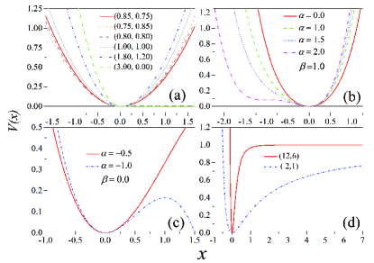
Figure 1: (Color lines) (a) to (d) are plots of potential of piecewise model, FPU-$\alpha$-$\beta$ model, FPU-$\alpha$ model, and L-J model, respectively.

We first study a two-particle system with the piecewise harmonic potential for the illuminating purpose. The equations of motion with periodic boundary conditions are

$$\begin{cases}\ddot{x}_{1}=k_{L,R}(x_{2}-x_{1})-k_{L,R}(x_{1}-x_{2})\\ \ddot{x}_{2}=k_{L,R}(x_{1}-x_{2})-k_{L,R}(x_{2}-x_{1})\end{cases},$$ (5)

and we assume $x_{1}(0)-x_{2}(0)<0$ while $t=0$, then Eq.5 can be rewritten as

$$\begin{cases}\ddot{x}_{1}=(k_{R}+k_{L})x_{2}-(k_{R}+k_{L})x_{1}\\ \ddot{x}_{2}=(k_{L}+k_{R})x_{1}-(k_{L}+k_{R})x_{2}\end{cases}.$$ (6)

In addition, momentum and energy are conserved, i.e., $p_{1}(t)+p_{2}(t)=0~{}\&~{}\frac{1}{2}p_{1}(0)^{2}+\frac{1}{2}p_{2}(0)^{2}+\frac{1}{2}k_{L}(x_{1}(0)-x_{2}(0))^{2}+\frac{1}{2}k_{R}(x_{2}(0)-x_{1}(0))^{2}=2\varepsilon$ (here $\varepsilon$ is mean energy of each particle). So we get $x_{1}(0)=-x_{2}(0)$, and $\varepsilon=\frac{1}{2}p_{1}(0)^{2}+(k_{L}+k_{R})x_{1}(0)^{2}=\frac{1}{2}p_{2}(0)^{2}+(k_{L}+k_{R})x_{2}(0)^{2}$. Then the results can been easily obtained and the simplified form is

$$\begin{cases}x_{1}(t)=\Lambda cos(2\sqrt{\bar{k}}t+\varphi)\\ x_{2}(t)=-\Lambda cos(2\sqrt{\bar{k}}t+\varphi)\end{cases},$$ (7)

where $\bar{k}=\frac{k_{L}+k_{R}}{2}$, $\Lambda=\sqrt{\frac{\varepsilon}{2\bar{k}}}$, $\varphi=-arctan(\frac{\sqrt{2}}{2\sqrt{\bar{k}}}\frac{p_{1}(0)}{x_{1}(0)})$. It’s easy to see the result does not depend on the initial conditions (if we assume $x_{1}(0)\geq x_{2}(0)$, we will get a same result).

We can clearly see the frequency of the system is $\omega=2\sqrt{\bar{k}}=2\sqrt{\bar{k}}sin(\frac{\pi}{2})$, which only relies on the mean value of $k_{L}$ and $k_{R}$ but has no direct dependency upon themselves. Besides, the frequency is completely same as that of the pure harmonic lattice KittelBook . It means that the piecewise linear two-particle system can be strictly described by a harmonic one with force constant $\bar{k}$.

For multi-particle situation

$$\omega=2\sqrt{\bar{k}}|sin(\frac{1}{2}aq)|$$ (8)

where $a$ is the lattice constant that is set be unit in our study, and $q$ is the wave-vector.

To verify our treatment for multi-particle cases, we immediately analyze the power spectrum of the time series of the particles’ instantaneous momentum by fast Fourier transformation (FFT) with molecular dynamics simulation (MDS). And the results are presented in Fig.2.

In Fig.2(a), the red solid line is power spectra of pure harmonic chain, i.e., to set $k_{L}=k_{R}$ in our model (here we set $k_{L}=k_{R}=1.0$). The green dot line is the theoretical position of frequency. It is clearly seen that our numerical results and existing theoretical results KittelBook are consistent, namely, our calculation program is completely accurate. Then we calculated our model and the results are shown in Fig.2(b) to (d). The blue solid (or red dash) line in Fig.2(b) is normalized power corresponding to $k_{L}=0.75~{}\&~{}k_{R}=0.85$ (or $k_{L}=0.85~{}\&~{}k_{R}=0.75$), and the green dot line is the theoretical value of frequencies’ centre position that is calculated by Eq.8. It is clearly seen that the theoretical and numerical results fit perfectly in all frequency regime. An interesting is that the two lines are almost complete overlap. This is due to exchanging the order of $k_{L}$ and $k_{R}$ does not affect the mean value of $\bar{k}$ (the two systems are mirror symmetrical). We also note that $\bar{k}$ does not rely on the temperature of system. The effect can be observed in Fig.2(c), where we did numerical experiments with fixed $k_{L}=1.8~{}\&~{}k_{R}=1.2$ under different energy density $\varepsilon=1.0,~{}10.0$. But the centre position of frequencies are still identical. At the same time, we find that the normalized (by energy density) power spectra overlap completely. This is because the model owns a similar certain scale that is pointed in Ref.ZhongYiCPB13 . Fig.2(d) shows an extremely asymmetric case ($k_{L}=3.0~{}\&~{}k_{R}=0.0$) that is very like a collision model. Strictly speaking, it is not a lattice but a fluid. But Eq.8 is still able to give a precise prediction for the centre positions of some low frequencies (the centre position of lowest frequency is identical with $k_{L}=1.8~{}\&~{}k_{R}=1.2$ because they have same mean value). It states that the piecewise linear system can be equivalent to a harmonic lattice with force constant $\bar{k}$, seriously.

To make a comparison from (a) to (d) in Fig.2, we can easily see that the phonon peak is broadening with asymmetry increasing (see the most typical examples Eq.8(c) and(d)). A similar phenomenon is also reported in Refs.ZhangyongarXiv2013 ; JunjiePRE2015 ; Zhangyong2015 . Therefore, here we emphasize that an asymmetric piecewise linear system can be well described by a pure harmonic lattice, only indicate that the centre positions of phonons peaks are same as an equivalent harmonic lattice, but there is essential difference comes from asymmetry between them, e.g., the phonon peak will broaden in true asymmetric piecewise linear lattice, which means that there exist stronger interactions between phonons. Besides, normal heat conduction is also observed in asymmetric harmonic model ZhongYiCPB13 , but these are absent in the equivalent pure harmonic chain.

All above presented results, the system size is fixed to $N=64$, so that we can clearly see all frequencies. But the correctness has been proved by our numerical experiment (not shown here) that is independent with system size.

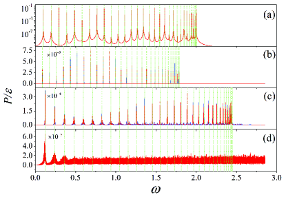
Figure 2: (Color lines) Normalized power spectra of the momentum time series. (a) The red solid line is corresponding to pure harmonic chain with $k_{L}=k_{R}=1.0$. (b) The blue solid (or red dash) line is corresponding to $k_{L}=0.75~{}\&~{}k_{R}=0.85$ (or $k_{L}=0.85~{}\&~{}k_{R}=0.75$). (d) the red solid corresponding $k_{L}=3.0~{}\&~{}k_{R}=0.0$. Energy density $\varepsilon$ is set be unit in these three simulations. (c) The blue solid line and red dash line are, respectively, corresponding to $\varepsilon=1.0,~{}10.0$ with fixed $k_{L}=1.8~{}\&~{}k_{R}=1.2$. The vertical green dot lines in all are predicted centre position of frequency. System size $N=64$ for all.

Up to now, we established our template model. For an unharmonic lattice, our goal is to obtain the two effective force constants. It is well known that the potential of a linear force ($F=-kx$) is $V=\frac{1}{2}kx^{2}$, which can easily obtained by $V=-\bar{F}x$ (here $\bar{F}=\frac{1}{2}F$ is the average force), and only the linear force has this nature. Based on this principle, we think that if a nonlinear force can be equivalent to a linear one, the equivalent potential should be also obtained by the same way, i.e., $\tilde{V}_{h}=\langle\frac{1}{2}\tilde{k}x^{2}\rangle=\langle-\bar{F}x\rangle$, and $\bar{F}=-\frac{1}{2}\frac{\partial V}{\partial x}$, the $\langle\cdots\rangle$ indicates the ensemble average. Further, we can get an specific equivalent approach as

$$\begin{cases}\tilde{k}_{L}=\frac{\langle\frac{\partial V}{\partial x}x\rangle}{\langle x^{2}\rangle},&x<0\\ \tilde{k}_{R}=\frac{\langle\frac{\partial V}{\partial x}x\rangle}{\langle x^{2}\rangle},&x\geq 0\\ \tilde{k}=\frac{\tilde{k}_{L}+\tilde{k}_{R}}{2}&\end{cases},$$ (9)

and above equations can be further rewritten as a general integral form

$$\tilde{k}=\frac{1}{2}\big{(}\frac{\int_{-\infty}^{0}\frac{\partial V}{\partial x}x\rho(x)dx}{\int_{-\infty}^{0}x^{2}\rho(x)dx}+\frac{\int_{0}^{\infty}\frac{\partial V}{\partial x}x\rho(x)dx}{\int_{0}^{\infty}x^{2}\rho(x)dx}\big{)},$$ (10)

where $\rho(x)=e^{-\frac{V(x)+Px}{k_{B}T}}$ is distribution function of relative displacement, $p=-\langle\frac{\partial V}{\partial x}\rangle$ is the thermodynamic pressureSpohnJSP14 ; SpohnarXiv2015 , and $k_{B}$ is Boltzmann constant that set to be unit, and $T$ is the temperature of system. Note that $\tilde{k}$ has a certain relationship with the speed of sound $c_{s}=\sqrt{\tilde{k}}$ in our dimensionless models. It is not a fixed constant but a function of temperature $T$ and system parameters. As a concrete example, FPU-$\alpha\beta$ model, $\tilde{k}=f(T,\alpha,\beta)$.

For symmetric FPU-$\beta$ model ($\alpha=0$) the pressure $p=0$, $V(x)$ and $\rho(x)$ will become even function, at this moment Eq.10 can be simplified as

$$\tilde{k}=\frac{\int_{-\infty}^{\infty}\frac{\partial V}{\partial x}x\rho(x)dx}{\int_{-\infty}^{\infty}x^{2}\rho(x)dx}.$$ (11)

A interesting observation is that Eq.11 is completely same as the form given in Ref.BaowenEPL2006 . So our tactics at least is effective for symmetric nonlinear models. In addition, from Eq.10 we can see that if the pressure is known, we can get the equivalent force constant $\tilde{k}$ through integration directly instead of MDS. Hence, it is necessary for us to find an approach to calculate the pressure. This goal is achived based on Spohn’s recent works SpohnJSP14 ; SpohnarXiv2015 ; SpohnPRL13 . Following these works we develop an algorithm for calculating the pressure of a momentum-conserved lattice as

$$\begin{cases}p=\frac{V(-\lambda)-V(\lambda)}{2\lambda}&(a)\\ \phi_{+}(\lambda)=\int_{0}^{\infty}xe^{-\frac{V(x)+px}{T}}dx&(b)\\ \phi_{-}(\lambda)=\int_{0}^{\infty}xe^{-\frac{V(-x)-px}{T}}dx&(c)\\ \phi(\lambda)=\phi_{+}(\lambda)-\phi_{-}(\lambda)\equiv 0&(d)\end{cases},$$ (12)

where $\lambda$ is an arguments that is governed by (d). Specific steps is to replace (a) into (b) and (c) in turn, then to solve the equation (d), after $\lambda$ is received the pressure will be easily obtained only need to put $\lambda$ back into (a). It is clearly seen that $\lambda$ is not unique but arbitrary for symmetric model. Nevertheless, arbitrary nonzero values of $\lambda$ put into the equation (a) will get fixed zero pressure, which just agree well with expectation of symmetric model. We should point out that if $\int_{-\infty}^{\infty}\rho(x)dx\rightarrow\infty$, the algorithm will do not work. The internal pressure and $\tilde{k}$ can only be acquired by MDS with Eq.9 (e.g., FPU-$\alpha$ model and L-J model).

In the following, we test whether Eq.10 is suitable for the asymmetric situation by the numerical integration. Here, we only need to check whether the prediction of the sound velocity accurately instead of calculating the centre position of lowest frequency by FFT. This is because Ref.ZhangyongarXiv2013 have proved that the shift of lowest frequency and the speed of sound are equal in dimensionless models. We compare our theoretical results (red uptriangle lines in Fig.3) with the standard sound velocity computed via the method developed by SpohnSpohnJSP14 ; SpohnarXiv2015 ; SpohnPRL13 (blue square lines in Fig.3, which can also be calculated by numerical integration). In order to make a comparison, we also show the result obtained with the traditional EPTBaowenEPL2006 (shorted as TEPT in the figure). All these are calculated by numerical integration instead of MDS, so they are independent of system size. One can see that the three methods get same results in low temperature regimes where the velocity is tending to one (gray dash line) and high temperature regimes $c_{s}\propto T^{1/4}$ (gray dot line, this can be also observed in Ref.HePRE2008 ). In the moderated temperature regimes, significant deviation appears with the traditional treatment, especially for large $\alpha$. In all the regimes, our theoretical predictions show no deviations.

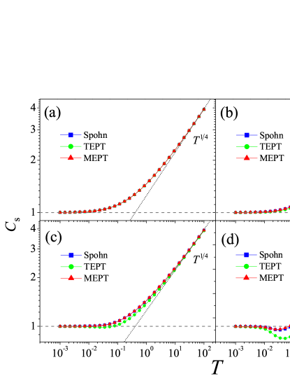
Figure 3: (Color lines) The speed of sound $c_{s}$ against temperature $T$ with different $\alpha=0.0(a),1.0(b),1.5(c)and2.0(d)$. Blue square line is calculated by Spohn’s formula, green circles are obtained by traditional EPT, and red uptriangles are achieved by our formula. $\beta=1.0$ is fixed throughly.

Next, we test it in FPU-$\alpha$ model and L-J model. For FPU-$\alpha$, we apply a small energy density $\varepsilon=0.01$ to avoid runaway instability of trajectories. The results are drawn in Fig. 4(a) for $\alpha=-0.5$, and Fig. 4(b) for $\alpha=-1.0$. For L-J model, $\varepsilon=0.5$ is fixed, and the results are shown in Fig.4(c) for $(m,n)=(12,6)$, and Fig.4(d) for $(m,n)=(2,1)$. From these results, we clearly see that our approach is very workable. And phonons peaks are broadening with asymmetry increasing as well in these models. Especially, it is clearly seen that the results of L-J model are vary similar to the result of a fluid (compare with Fig. 2(d), normal heat conduction is observed in both of themshunda_arXiv2012 ; ZhongYiCPB13 ).

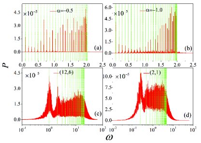
Figure 4: (Color lines) Power spectra of the momentum time series. (a) and (b) for FPU-$\alpha$ model, $\varepsilon=0.01$. (c) and (d) for L-J model, $\varepsilon=0.5$. The vertical green dot lines are predicted centre positions of frequencies. System size is fixed at $N=64$.

To summarize, we present an effective phonon treatment that works very well in one dimensional momentum-conserved lattice with either symmetric or asymmetric interaction potentials. In asymmetric models, all phonons peaks are broaden, and the degree of the broaden depends on the degree of the potential asymmerty. The more stronger the asymmetry, the more stronger the phonon scattering. This effect may explain why the normal heat conduction behavior appears in certain lattice models ZhongYiCPB13 ; shunda_arXiv2012 ; ZhongYiPRE12 ; Savin14PRE. We shall discuss this problem in a forthcoming paper Weicheng02 .

References

- (1) S. Lepri, R. Livi, and A. Politi, Phys. Rep. 377, 1 (2003).
- (2) A. Dhar, Adv. Phys. 57, 457 (2008).
- (3) N. Li, J. Ren, L. Wang, G. Zhang, P. Hänggi, and B. Li, Rev. Mod. Phys. 84, 1045 (2012).
- (4) G. P. Srivastave, The Physics of Phonons (IOP, Bristol, 1990).
- (5) C. Alabiso, M. Casrtelli, and P. Marenzoni, J. Stat. Phys. 79, 451 (1995).
- (6) S. Lepri, Phys. Rev. E 58, 7165 (1998).
- (7) B. Gershgorin, Yuri V. Lvov, and D. Cai, Phys. Rev. Lett. 95, 264302 (2005).
- (8) B. Gershgorin, Yuri V. Lvov, and D. Cai, Phys. Rev. E 75, 046603 (2007).
- (9) N. Li, P. Tong, and B. Li, Europhys. Lett. 75, 49 (2006).
- (10) N. Li, and B. Li, Europhys. Lett. 78, 34001 (2007).
- (11) D. He, S. Buyukdagli, and B. Hu, Phys. Rev. E 78, 061103 (2008).
- (12) N. Li, B. Li, and S. Flach, Phys. Rev. Lett. 105, 054102 (2010).
- (13) S. Liu, J. Liu, P. Hänggi, C. Wu, and B. Li, Phys. Rev. B 90, 174304 (2014).
- (14) Y. Zhang, S. Chen, J. Wang, and H. Zhao, arXiv:1301.2838.
- (15) E. Fermi, J. Pasta, S. Ulam, and M. Tsingou, Los Alamos preprint LA-1940 (1955).
- (16) C. Kittel, Introduction to Solid State Physics (8ed., Wiley,2005).
- (17) Y. Zhong, Y. Zhang, J. Wang, and H. Zhao, Chin. Phys. B 22, 070505 (2013).
- (18) Y. Zhang, J. Wang, and H. Zhao (to be pubilshed).
- (19) J. Liu, S. Liu, N. Li, B. Li, and C. Wu, Phys. Rev. E 91, 042910 (2015).
- (20) H. Spohn, J. Stat. Phys. 154, 1191 (2014).
- (21) H. Spohn, arXiv:1505.05987.
- (22) C. B. Mendl, and H. Spohn, Phys. Rev. Lett. 111, 230601 (2013).
- (23) S. Chen, Y. Zhang, J. Wang, and H. Zhao, arXiv:1204.5933.
- (24) Y. Zhong, Y. Zhang, J. Wang, and H. Zhao, Phys. Rev. E 85, 060102 (2012).
- (25) W. Fu, Y. Zhang, H. Zhao. (unpublished).