Spectrum Reservation Contract Design in TV White Space Networks

Abstract

In this paper, we study a broker-based TV white space market, where unlicensed white space devices (WSDs) purchase white space spectrum from TV licensees via a third-party geo-location database (DB), which serves as a spectrum broker, reserving spectrum from TV licensees and then reselling the reserved spectrum to WSDs. We propose a contract-theoretic framework for the database’s spectrum reservation under demand stochasticity and information asymmetry. In such a framework, the database offers a set of contract items in the form of reservation amount and the corresponding payment, and each WSD chooses the best contract item based on its private information. We systematically study the optimal reservation contract design (that maximizes the database’s expected profit) under two different risk-bearing schemes: DB-bearing-risk and WSD-bearing-risk, depending on who (the database or the WSDs) will bear the risk of over reservation. Counter-intuitively, we show that the optimal contract under DB-bearing-risk leads to a higher profit for the database and a higher total network profit.

I Introduction

I-A Background and Motivations

Nowadays, radio spectrum is becoming more congested and scarce with the explosive development of wireless services and networks. Dynamic spectrum sharing can effectively improve the spectrum efficiency and alleviate the spectrum scarcity, by allowing unlicensed secondary devices access to the licensed spectrum in an opportunistic manner. TV white space network is one of the promising paradigms of dynamic spectrum sharing [2, 3], where unlicensed devices (called white space devices, WSDs) exploit the un-used or under-utilized broadcast television spectrum (called TV white spaces, TVWS) opportunistically.

In order to fully utilize TVWS while not harming licensed devices, regulatory bodies (e.g., FCC in the US and Ofcom in the UK) have advocated a database-assisted spectrum access solution, which relies on a third-party white space database called geo-location [3, 2]. In this solution, WSDs obtain the available spectrum information through querying the geo-location database, instead of performing spectrum sensing. More specifically, WSDs periodically report their location information and other optional information (e.g., spectrum demand) to a geo-location database, and then the database returns the available spectrum in the respective locations and time periods to WSDs.

In general, there are two types of different TV white space spectrum resources. The first type is the TV spectrum not registered to any TV licensee or Programme Making and Special Events (PMSE) at a particular location. This type of spectrum is usually for the open and shared usage among unlicensed WSDs, according to the regulators’ policies [2]. The second type is the TV spectrum already registered to some TV licensees and PMSE, but not fully utilized by those licensees. Hence, the licensees can temporarily lease these idle spectrum to unlicensed WSDs for the exclusive usage. In such a secondary spectrum market, the geo-location database can act as an intermediary (e.g., a broker) between the licensees (sellers) and the WSDs (buyers), due to its proximity to both sides of the market.

In this work, we focus on the secondary sharing and trading of the second type spectrum resource, i.e., those registered but under-utilized spectrum. Such spectrum can be exclusively used by a WSD (with the permission of the licensees), hence are particularly suitable for supporting applications that require a high QoS.

I-B Market Model and Problem

Figure 1: Broker-based spectrum reservation market. In Step 0, the geo-location database (broker) reserves spectrum from TV licensees and PMSE for every reservation period (e.g., one day). In Step 1, each WSD (master) reports its location and demand in every access period (e.g., one hour). In Step 2, the database sells the corresponding spectrum to the WSD in every access period. In Step 3, the WSD serves end-users (slaves) in every access period using the obtained spectrum. Notice that Steps 1-3 will occur repeatedly within every reservation period, as one reservation period consists of many access periods.

Specifically, we study a broker-based secondary spectrum market, where TV licensees lease their idle spectrum to unlicensed WSDs via a spectrum broker acted by a geo-location database. As a broker, the database purchases spectrum from TV licensees in advance, and then resells the leased spectrum to WSDs. Figure 1 illustrates such a broker-based spectrum reservation market model. As the TV towers have fixed locations and TV programs have well planned schedules, the reservation period of TV spectrum can be relative long [8]. Thus, we model and analyze a spectrum reservation market, where the database reserves spectrum from TV licensees in advance for a relatively large time period (e.g., more than one day), called the reservation period. Then, within each reservation period, the database sells the reserved spectrum to WSDs periodically with a relatively small time period (e.g., one hour), called the access period. Namely, the spectrum reservation decision is made at the beginning of the reservation period, which consists of many access periods.

In such a spectrum reservation market, the database needs to reserve spectrum in advance, without knowing the actual future demands from WSDs. Therefore, an important problem for the database in this market is:

• How much bandwidth should the database reserve for each WSD, aiming at maximizing the database’s profit?

The problem is challenging due to the demand stochasticity and the information asymmetry.

(i) Demand Stochasticity. Due to the stochastic nature of end-users’ activities and requirements, each WSD’s spectrum demand (for serving its end-users) is a random variable, and cannot be precisely predicted by the WSD or the database in advance. Therefore, there is inevitably a risk of reservation mismatch, e.g., spectrum over-reservation or under-reservation. Accordingly, the database’s spectrum reservation decision depends on the risk-bearing scheme, namely, who will bear the risk of spectrum over-reservation: the database (called DB-bearing-risk) or the WSD (called WSD-bearing-risk)? In the former case, the WSD only pays for the spectrum it actually purchases in every access period; while in the latter case, the WSD has to pay for the reserved spectrum(even if it is more than actually needed) in every access period.

(ii) Information Asymmetry. The above mentioned demand information is asymmetric between the database and WSDs. Due to the proximity to end-users, the WSD usually has more information (i.e., with less uncertainty) about the spectrum demand than the database. This implies that the database can potentially make a better reservation decision, if it is able to know the WSD’s private information regarding the demand. However, without proper incentives, the WSD may not be willing to share its private information with the database. As will be shown in Section 5, the WSD may even report a false information to the database intentionally, as long as such a misreport can increase the WSD profit.

I-C Results and Contributions

We propose a contract-theoretic spectrum reservation framework, in which the database offers a list of contract items in the form of reservation amount and the corresponding payment, and each WSD chooses the best contract item based on its private demand information (from its served end-users). We first study the incentive compatible contract design, under which each WSD will disclose its private demand information credibly, by choosing the contract item intended for its private information. With the incentive compatibility, we further derive the optimal spectrum reservation contracts that maximize the database expected profit under both DB-bearing-risk and WSD-bearing-risk schemes. For clarity, we summarize the key results regarding the optimal contract design in Table I.

As far as we know, this is the first paper that systematically studies the contract-based spectrum reservations under different risk-bearing schemes for TV white space markets. The proposed market model, together with the derived spectrum reservation solutions, can offer the proper economic incentives for the database operator, and support the practical and commercial deployment of TV white space networks. The main contributions of this paper are summarized as follows.

• Novel modeling and solution techniques: We study a generic spectrum reservation market under demand stochasticity and information asymmetry, and propose a contract-theoretic reservation framework, which ensures that WSDs disclose their private information truthfully, and meanwhile maximizes the database profit.

• Optimal contract design: We analytically derive the optimal spectrum reservation contract design under DB-bearing-risk and WSD-bearing-risk schemes, and numerically compare their performances. Through these numerical comparisons, we characterize the impacts of risk-bearing scheme, demand stochasticity, and information asymmetry on the spectrum reservation solutions.

• Numerical results and insights: Our numerical results show that the optimal contract under the DB-bearing-risk scheme can achieve a higher database profit and a higher total network profit, compared to the optimal contract under the WSD-bearing-risk scheme. The intuition is that the WSD is more risk-averse than the database.

TABLE I: Key Results in This Paper

Risk-Bearing	Information & Sharing		Spectrum Reservation Decision	Solution	Section
	Symmetry (Benchmark)	—	The database makes the reservation decision based on the WSD’s knowledge about demand.	$k_{\textsc{(i)}}^{\textsc{sym}}$ in Eq. (6)	V-A1
DB-Bearing-Risk (Scheme I)	Asymmetry (Benchmark)	No Sharing	The database makes the reservation decision based on its own knowledge about demand.	$k_{\textsc{(i)}}^{\textsc{asy}}$ in Eq. (8)	V-A2
	Asymmetry (Our Focus)	Credibly Sharing via Contract	The database offers a spectrum reservation contract, and each WSD chooses a proper contract item (reservation-payment pair).	$k_{\textsc{(i)}}^{*}$ in Theorem 1	VI-A
	Symmetry (Benchmark)	—	Each WSD makes the reservation decision based on its knowledge about demand.	$k_{\textsc{(ii)}}^{\textsc{sym}}$ in Eq. (11)	V-B1
WSD-Bearing-Risk (Scheme II)	Asymmetry (Benchmark)	No Sharing	Each WSD makes the reservation decision based on its knowledge about demand.	$k_{\textsc{(ii)}}^{\textsc{asy}}$ in Eq. (12)	V-B2
	Asymmetry (Our Focus)	Credibly Sharing via Contract	The database offers a spectrum reservation contract, and each WSD chooses a proper contract item (reservation-payment pair).	$k_{\textsc{(ii)}}^{*}$ in Theorem 2	VI-B

The rest of this paper is organized as follows. In Section II, we review the related literature. In Section III, we present the system model. In Sections IV, we provide the integrated optimal reservation solution as a benchmark. In Sections V and VI, we study the decentralized spectrum reservations without information sharing and with information sharing (via contract), respectively. We provide numerical results in Section VII, and finally conclude in Section VIII.

II Related Work

In the recent regulator’s policy [6], the databases are allowed to determine their own pricing schemes for operating the TVWS. This motivates researchers to study the economic issues in TVWS[13, 14, 15, 16, 17, 18, 19]. In [13], Feng et al. studied the hybrid pricing scheme for the database manager. In [14], Luo et al. studied the pricing strategy of oligopoly competitive WSDs. However, none of the existing work considered the bandwidth reservation problem under information asymmetry. Some recent studies [15, 16, 17, 18, 19] proposed the pure and hybrid information models for TV white spaces, which focus on unlicensed TV white space.

Our work is related to the supply chain contract design in the operations management and marketing science literature. Supply chain contract is widely used as a mechanism to coordinate production quantity and pricing, so that the performance of decentralized supply chain is close or the same as that of an integrated one. In [9], Cachon et al. considered the stochastic nature of demand and prescribed analytical remedies for credible information sharing between a supplier and a manufacturer. $\ddot{O}$zer et al. in [10] extended Cachon’s work and further examined how a supplier can screen buyers’s private information by offering a menu of contracts. However, the above work considered the case where the contract designer bears all of the risk of over-reservation. We consider both cases where the contract designer (the database) and the buyer (WSD) bears the risk of over-reservation, respectively.

Recently, the concept of contract was also introduced into the spectrum trading model (e.g. [20, 21, 22]). In [20], Gao et al. proposed a quality-price contract for the spectrum trading in a monopoly spectrum market. In [21], Duan et al. proposed a contract-based cooperative spectrum sharing mechanism to promote the cooperation of a primary user and a secondary user. In [22], Sheng et al. proposed a contract for a primary license holder to sell its excess spectrum capacity to potential secondary users. In this paper, we propose a contract-based mechanism for the spectrum reservation problem. In our model, the demand of a WSD consists of two parts: one is unknown by both the database and the WSD, and the other is only known by the WSD (hence is the WSD’s private information). Thus, the optimal contract design needs to consider not only the truthful information disclosure of the WSD, but also the uncertainty of demand for both the database and the WSD. This makes our contract design much more challenging than existing contract designs.

III System Model

III-A System Overview

We consider a TV white space network where unlicensed WSDs exploit the under-utilized broadcast television spectrum (called TV white space, or spectrum for simplicity) via a geo-location database. Each WSD is an infrastructure-based device (e.g., a base station), and serves a set of unlicensed end-users/devices called “slave” devices. We assume that the number of unlicensed WSDs is large enough, so that the spectrum demand of a particular WSD does not affect other WSDs’ demand. This allows us to concentrate on the interaction between the database and each WSD.

We focus on the secondary sharing and trading of the under-utilized licensed spectrum of TV licensees. In particular, we model a broker-based secondary spectrum market, where the geo-location database acts as a spectrum broker, reserving spectrum from TV licensees in advance and then reselling the reserved spectrum to unlicensed WSDs.

III-B Broker-based Spectrum Reservation Market

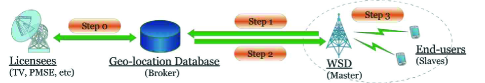
Figure 2: Spectrum reservation and access processes. Step 0: the database reserves spectrum for every reservation period $T$; Step 1: the WSD reports the realized demand in every access period $t$; Step 2: the database returns spectrum to the WSD in every access period $t$; Step 3: the WSD serves end-users in every access period $t$.

Now we discuss the proposed spectrum reservation market more detailedly. Let $c$ denote the unit price (cost) at which the database reserves spectrum from TV licensees. Let $w$ denote the unit price (wholesale price) at which the database sells spectrum to the WSD. Let $r$ and $s$ denote the unit price (market price) at which the WSD serves the subscribed and un-subscribed end-users, respectively. In order to concentrate on the spectrum reservation problem, we consider a fixed spectrum trading model, that is, the trading prices $c,\ w,\ r,$ and $s$ are fixed system parameters. This implies that our proposed spectrum reservation framework does not need to alter the spectrum trading process, and thus is compatible with many existing spectrum market mechanism designs. Moreover, to make the trading model meaningful, we assume that $\min\{r,s\}>w>c$, i.e., both the database and the mater will benefit from the trading process.

We illustrate the detailed spectrum reservation and trading/access processes in Figure 2 and Algorithm 1. It is notable that the spectrum reservation process (Step 0) is performed at a relatively large time period (e.g, oncen every day or every week), called the reservation period (denoted by $T$); while the spectrum trading/access processes (Steps 1-3) are performed at a relatively small time period (e.g., once per hour), called the access period (denoted by $t$).

for each reservation period $T=1,2,\ldots$ do

      Step 0: The database reserves $k$ unit of spectrum from TV licensees at a unit price $c$, for each reservation period; for each access period $t=1,...,T$ do

             Step 1: The WSD collects the realized end-user demand $d$, and requests $d$ units of spectrum from the database in each access period;

             Step 2: The database sells $\min\{k,d\}$;

             Step 3: The WSD serves end-users using the received spectrum at a market price $r$ or $s$ in each access period.

       end for

      

end for

Algorithm 1 Algorithmic statement for the three-stage hierarchical model.

We focus on the following database’s spectrum reservation problem: how to determine the proper spectrum reservation amount $k$ to maximize the database profit? The problem is challenging due to the demand stochasticity (see Section III-C) as well as the information asymmetry (see Section III-D). Moreover, the spectrum reservation decision also depends on the risk-bearing scheme (see Section III-E), namely, who (i.e., the database or the WSD) will bear the risk of spectrum over-reservation. This further complicates the problem.

III-C Demand Stochasticity

In each access period, a WSD $n\in\mathcal{N}$ uses the purchased spectrum to serve its end-users. We consider two types of end-users for each WSD: registered end-users (called subscribers) and unregistered end-users (called random access users or random users). Let $\mathcal{J}_{n}$ and $\mathcal{I}_{n}$ denote the sets of WSD $n$’s subscribers and random users, respectively.

Specifically, subscribers characterize the residents in the WSD’s serving area, and these users can sign a service contract with the WSD in advanced. Because of this, the WSD has a good knowledge regarding the demand of these users based on the long-term interactions. The random end-users characterize the travelers to the WSD’s serving area, and these users do not have any prior contractual relationship with the WSD. It is difficult for the WSD to predict the demand from these users. Naturally, we assume that subscribers have a higher priority in obtaining service than random users. That is, when the spectrum received by the WSD (from the database) is not enough to meet all end-users’ demand, the WSD will satisfy the subscribers’s demand first, and then serve the random users using the remaining spectrum. Recall that $r$ and $s$ are the unit prices (of spectrum) for serving subscribers and random users, respectively. Due to the high priority of subscribers, it is reasonable to assume that $r>s$.

Let $\xi_{n,j}$ and $\varepsilon_{n,i}$ denote the spectrum demands of a subscriber $j\in\mathcal{J}_{n}$ and a random user $i\in\mathcal{I}_{n}$ (to WSD $n$) in one access period, respectively. We assume that (i) $\xi_{n,j}$ keeps unchanged within each reservation period $T$ (but may vary across $T$), which implies that each contract’s validity is larger than one access period; and (ii) $\varepsilon_{n,i}$ keeps unchanged within each access period $t$ (but may vary across $t$), which implies that each random user’s average QoS and wireless characteristic remain constant in each access period. The total demand (of all subscribers and random users) of WSD $n$ in one access period is:

$$\textstyle d_{n}=\sum_{j\in\mathcal{J}_{n}}\xi_{n,j}+\sum_{i\in\mathcal{I}_{n}}\varepsilon_{n,i}\triangleq\xi_{n}+\varepsilon_{n},$$ (1)

where $\xi_{n}\triangleq\sum_{j\in\mathcal{J}_{n}}\xi_{n,j}$ is total subscriber demand, and ${\varepsilon_{n}}\triangleq\sum_{i\in\mathcal{I}_{n}}\varepsilon_{n,i}\triangleq\xi_{n}$ is total random user demand. For convenience, we refer to $\xi_{n}$ as the scheduled demand of WSD $n$ (as it is known at the beginning of each reservation period, and keeps unchanged during the whole reservation period), and refer to ${\varepsilon_{n}}$ as the bursty demand of WSD $n$ (as it is known only at the beginning of each access period, and changes randomly in different access periods).

Based on the assumptions mentioned above, the scheduled demand $\xi_{n}$ is a random variable changing each reservation period $T$, and the bursty demand $\varepsilon_{n}$ is a random variable changing each access period $t$. For simplicity, we assume that $\xi_{n}$ and $\varepsilon_{n}$ are independent and identically distributed (i.i.d) in different reservation periods and access periods, respectively. Let $f(\xi)$ and $F(\xi)$ denote the probability density function (pdf) and cumulative distribution function (cdf) of $\xi$, and $g(\varepsilon)$ and $G(\varepsilon)$ denote the pdf and cdf of $\varepsilon$, respectively. As in many mechanism design literature (see, e.g., [20, 21, 22]), we assume that such distribution information are public information to both the database and the WSD. In practice, they can be obtained through machine learning in a sufficiently long time period. As mentioned previously, the number of WSDs is large enough so that one WSD’s strategy is independent of others. Hence, we can concentrate on the interaction between the database and one WSD.

Since the total demand $d$ changes randomly in each access period $t$, while the spectrum reservation is performed at the beginning of each reservation period $T$, the database or the WSD faces a spectrum reservation problem under demand stochasticity. Obviously, a higher reservation can serve more demand potentially, but may also lead to a higher risk of spectrum over-reservation. A lower reservation, however, may lead to a higher loss due to the spectrum under-reservation.

Next we draw some useful properties of the scheduled demand $\xi$ and the bursty demand $\varepsilon$. First, we notice that the random users’ bursty demand usually depends on the real-time market price $s$ and end-users’ wireless characteristics. As an example commonly used in the networking literature (e.g., [1]-[23]), a random user $i$’s utility $\pi_{i}$ can be defined as the difference between the achiavable data rate (e.g., the Shannon capacity assuming high SNR [24]) and the payment, e.g.,

$$\textstyle\pi_{i}=\beta\cdot\varepsilon_{i}\cdot\ln\left(\frac{P_{i}|h_{i}|^{2}}{\varepsilon_{i}n_{0}}\right)-s\cdot\varepsilon_{i},\vspace{-1mm}$$

where $\left|h_{i}\right|$ is the channel gain, $P_{i}$ is the transmission power, $n_{0}$ is the noise power per unit bandwidth, and $\beta$ denotes the monetary income per unit of data rate. Based on the above utility definition, the optimal bursty demand for a random user $i$ that maximizes its payoff $\pi_{i}$ is

$$\textstyle\varepsilon_{i}=\frac{P_{i}\cdot e^{-{(1+s/\beta)}}\cdot|h_{i}|^{2}}{n_{0}}.$$

Notice that the channel coefficient $h_{i}$ satisfies: (i) $h_{i}\sim\mathcal{C}(0,1)$, the complex normal distribution (when the channel experiences the Rayleigh fading), and (ii) $h_{i}$ is i.i.d for different users $i\in\mathcal{I}_{n}$. Therefore, both $\varepsilon_{i}$ and $\varepsilon$ follow the chi-square distribution [24] (with different degrees of freedom). Note, however, that our analysis also holds for other demand distributions such as the normal distribution.

Second, the subscribers’ scheduled demand $\xi$ is a long-term average demand (changing every reservation period, e.g., one day), and usually independent of the short-term wireless characteristics. Our analysis holds for arbitrary $\xi$ distribution with the increasing failure rate (IFR), i.e., $\frac{f(\xi)}{1-F(\xi)}$ is increasing in $\xi$.

III-D Information Asymmetry

Due to the different proximities to end-users, the database and the WSD usually have different knowledge about the scheduled demand $\xi$ and the bursty demand $\varepsilon$. Table LABEL:table:information illustrates the difference between the database’s knowledge and the WSD’s knowledge regarding the end-user demand at the beginning of each reservation period $T$ (when making the reservation decision). Specifically,

• Bursty demand $\varepsilon$ of random users: Notice that $\varepsilon$ changes randomly every access period. Thus, neither the WSD nor the database knows the exact value of $\varepsilon$ at the beginning of the reservation period. That is, both the WSD and the database only know the distribution of ${\varepsilon}$.

• Scheduled demand $\xi$ of subscribers: Notice that $\xi$ keeps unchanged within each reservation period. Thus, the WSD is able to know the exact value of $\xi$ (e.g., through bilateral agreements signed with subscribers) at the beginning of the reservation period. The database, however, does not know the exact value of $\xi$ unless the WSD shares such information. That is, the database only knows the distribution of ${\xi}$.

We refer to the difference between the database’s knowledge and the WSD’s knowledge regarding demand information as information asymmetry. The co-existence of these two types of end-users and the information asymmetry provide incentives for the WSD to misreport its private information. Without the existence of random users, the WSD would request the database to reserve spectrum equal to the demand of subscribed users. With the existence of random end-users, the WSD would reserve the amount of spectrum larger than the demand of subscribed end-users, in order to gain more revenue by serving both the subscribed end-users and the random end-users. However, the exact value of the random end-users demand is unknown by the WSD at the beginning of the reservation period. Hence, to maximize its own profit, the WSD would optimize the value to be reported to the database, instead of truthfully revealing his information of the certain demand of subscribed users. Such strategic misreporting will make it difficult for the database to make the optimal reservation decision to maximize the database’s payoff. To hedge information asymmetry, it is important to design an incentive compatible mechanism to elicit the WSD’s private demand information (i.e., $\xi$). In this work, we will propose contract-theoretic spectrum reservation mechanisms to achieve this goal.

III-E Risk-Bearing Scheme

Due to the demand stochasticity, there is a risk of spectrum over-reservation. Thus, the spectrum reservation decision depends greatly on the risk-bearing scheme. Namely, who will bear the risk of spectrum over-reservation, i.e., the database or WSDs? We refer to the former scheme as DB-bearing-risk (Scheme I) and the latter scheme as WSD-bearing-risk (Scheme II). Specifically,

• DB-bearing-risk (Scheme I): In this case, the WSD only pays for the spectrum it actually purchases in each access period, and thus the database bears all the risk of spectrum over-reservation. That is, in each access period, the WSD will only pay for $\min\{k,d\}$ units of spectrum that it consumes.

• WSD-bearing-risk (Scheme II): In this case, the WSD pays for all the spectrum reserved, and thus the WSD bears all the risk of spectrum over-reservation. That is, in each access period, the WSD will pay for all $k$ units of reserved spectrum, even if the total demand $d$ is smaller than $k$.

In this paper, we will study the spectrum reservation problem under both risk-bearing schemes systematically. In the following sections, we first study the centralized/integrated spectrum reservation solution as a (centralized) benchmark (Section IV). Then we study the decentralized reservation solution without information sharing as another (decentralized) benchmark (Section V), and show that it may lead to a poor performance (in terms of database profit and network profit) due to the asymmetry of information. To this end, we study the decentralized reservation solution with contract-based credible information sharing (Section VI). To facilitate the understanding, we have listed the key results of this work in Table I.

IV Integrated spectrum Reservation Solution

In this section, we consider an integrated system, where the database and the WSD act as an integrated decision maker to maximize their aggregate profit (called network profit, denoted by $\Pi$). We will study this integrated/centralized optimal spectrum reservation as the centralized benchmark.

Obviously, in this case the integrated player (database and WSD) knows the precise value of $\xi$ and the distribution of ${\varepsilon}$. Moreover, there is no difference between the DB-bearing-risk scheme and the WSD-bearing-risk scheme. Specifically, given any spectrum reservation $k$, the expected network profit is

$$\textstyle\Pi(k,\xi)= r\cdot{\min{\{k,\xi\}}}+s\cdot\mathbb{E}_{\varepsilon}\big{[}\min\big{\{}{\varepsilon},(k-{\xi})^{+}\big{\}}\big{]}-c\cdot{k},$$ (2)

where $(x)^{+}=\max\{x,0\}$. This formula implies that the WSD will satisfy the subscribers’ scheduled demand first (1st term), and then satisfy the random users’ bursty demand using the remaining spectrum (2nd term).

Next we study the centralized optimal reservation $k^{\circ}$ that maximizes the network profit defined in (2). Notice that when $k\leq\xi$, we have $\frac{\partial{\Pi(k,\xi)}}{\partial{k}}=r-c>0$, which implies that the optimal $k$ cannot be smaller than $\xi$; when $k\geq\xi$, we have (i) $\frac{\partial{\Pi(k,\xi)}}{\partial{k}}=s\big{[}1-G(k-\xi)\big{]}-c$, and (ii) $\frac{\partial^{2}{\Pi(k,\xi)}}{\partial{k}^{2}}=-s\cdot g\big{(}k-\xi\big{)}\leq 0$. Thus, the centralized optimal reservation $k^{\circ}$ is given by the first-order condition $\frac{\partial{\Pi(k,\xi)}}{\partial{k}}=0$, and more formally,

$$\textstyle k^{\circ}=\xi+{G^{-1}\Big{(}\frac{s-c}{s}\Big{)}}.\vspace{-1mm}$$ (3)

Intuitively, $k^{\circ}$ consists of two parts: (i) the scheduled demand $\xi$, and (ii) the best response to the bursty demand $\varepsilon$. Note that the centralized optimal reservation $k^{\circ}$ is a function of $\xi$, but not a function of $\varepsilon$. This is because the integrated player knows the precise value of $\xi$, but not the value of $\varepsilon$.

V Decentralized spectrum Reservation – No Information Sharing

Now we consider a general decentralized system, where the database and the WSD make decisions independently, aiming at maximizing their individual profits. In this section, we will study the decentralized spectrum reservation solution under information symmetry and under information asymmetry without information sharing as the decentralized benchmarks.

V-A Scheme I: DB-Bearing-Risk

Under the DB-bearing-risk scheme, the WSD only pays for the spectrum it actually uses, and thus the database bears all the risk of spectrum over-reservation. That is, in each access period, the WSD will only purchase $\min\{k,d\}$ units of spectrum.

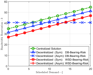
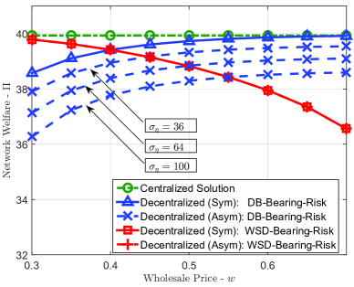
Figure 3: (a) Spectrum Reservation vs Scheduled Demand $\xi$, and (b) Network Profit vs Wholesale Price $w$. Here, $\sigma_{\xi}$ denotes the variance of the scheduled demand $\xi$.

.

V-A1 Information Symmetry

We first study the database’s optimal spectrum reservation solution under information symmetry, where the database is assumed to know the precise value of $\xi$. Specifically, for any reservation $k$, the WSD’s and the database’s (ex-ante) expected profits are, respectively,

$$\textstyle\pi_{\textsc{ms}}(k,\xi)= (r-w)\cdot\min\{k,\xi\}$$ (4)

$$\quad{}+(s-w)\cdot\mathbb{E}_{\varepsilon}\big{[}\min\big{\{}{\varepsilon},(k-\xi)^{+}\big{\}}\big{]},$$

$$\textstyle\pi_{\textsc{db}}(k,\xi)=w\cdot\mathbb{E}_{\varepsilon}\big{[}\min\{\varepsilon+\xi,k\}\big{]}-c\cdot{k}.~{}~{}~{}~{}~{}~{}~{}~{}~{}~{}~{}~{}~{}~{}~{}~{}~{}~{}~{}~{}~{}~{}~{}~{}~{}~{}~{}~{}~{}~{}~{}$$ (5)

The optimal reservation for the database (i.e., that maximizes its profit defined in (5)) is

$$\textstyle k_{\textsc{(i)}}^{\textsc{sym}}=\xi+{G^{-1}\Big{(}\frac{w-c}{w}\Big{)}}.$$ (6)

Similar to the centralized optimal reservation $k^{\circ}$, the above decentralized optimal reservation $k_{\textsc{(i)}}^{\textsc{sym}}$ under information symmetry is also a function of $\xi$.

V-A2 Information Asymmetry

In practice, the demand information is asymmetric between the database and the WSD as discussed in Section III-D. Now we study the database’s optimal spectrum reservation solution under information asymmetry, where the database does not know the precise value of $\xi$.

We first show that the reservation solution $k_{\textsc{(i)}}^{\textsc{sym}}$ in (6) under information symmetry may not be the database’s optimal solution in this case, as it cannot ensure that the WSD shares its private information $\xi$ with the database credibly. Notice that (i) the WSD profit $\pi_{\textsc{ms}}(k,\xi)$ in (4) increases with the spectrum reservation $k$, and (ii) the database’s optimal spectrum reservation $k_{\textsc{(i)}}^{\textsc{sym}}$ in (6) is linear to $\xi$. This implies that the WSD has an incentive to inflate its private information $\xi$. The key reason behind this phenomenon is that the database bears all the risk of over-reservation.

As a consequence, the database will not trust the information (i.e., the value of $\xi$) informed by the WSD, and therefore will act based on its own prior distribution information of $\xi$ and $\varepsilon$. That is, it will maximize the following expected profit:

$$\bar{\pi}_{\textsc{db}}(k)\triangleq\mathbb{E}_{\xi}\big{[}\pi_{\textsc{db}}(k,\xi)\big{]}=w\cdot\mathbb{E}_{\xi,\varepsilon}\big{[}\min\{\varepsilon+\xi,k\}\big{]}-c\cdot{k},$$ (7)

where the expectation $\mathbb{E}_{\xi,\varepsilon}$ is taken over the distribution of $\xi$ and $\varepsilon$. The optimal reservation for the database that maximizes its expected profit defined in (7) is

$$\textstyle k_{\textsc{(i)}}^{\textsc{asy}}=(F\times G)^{-1}\Big{(}\frac{w-c}{w}\Big{)},$$ (8)

where $F\times G$ is the joint c.d.f. of $\xi+{\varepsilon}$.

Note that $k_{\textsc{(i)}}^{\textsc{asy}}$ is not a function of $\xi$, which is different from (3) and (6). This implies that the database cannot adjust its spectrum reservation decision to account for the WSD’s private information. Therefore, both parties’s profits may reduce due to the ignorance of information $\xi$ (that WSD has) in the spectrum reservation. To solve this problem, we will propose a spectrum reservation contract to achieve the credible information sharing between the database and the WSD in Section VI-A.

V-B Scheme II: WSD-Bearing-Risk

Under the WSD-bearing-risk scheme, the WSD pays for all the spectrum reserved, and thus the WSD bears all the risk of spectrum over-reservation. That is, in each access period, the WSD will pay for all $k$ units of reserved spectrum, even if the total demand $d$ is smaller than $k$.

V-B1 Information Symmetry

Similarly, we first study the WSD’s optimal spectrum reservation decision under information symmetry. Specifically, for any reservation $k$, the WSD’s and the database’s (ex-ante) expected profits are, respectively,

$$\textstyle\pi_{\textsc{ms}}(k,\xi)= r\cdot\min\{k,\xi\}+s\cdot\mathbb{E}_{\varepsilon}\big{[}\min\big{\{}{\varepsilon},(k-\xi)^{+}\big{\}}\big{]}-wk,$$ (9)

$$\textstyle\pi_{\textsc{db}}(k,\xi)=(w-c)\cdot{k}.{}{}{}{}{}{}{}{}{}{}{}{}{}{}{}{}{}{}{}{}{}{}{}{}{}{}{}{}{}{}$$ (10)

Note that if the WSD bears the risk, then the WSD will determine the spectrum reservation amount. Otherwise, the database will always choose a very large reservation as it does not bear the risk of over-reservation. Accordingly, the optimal reservation for the WSD (i.e., that maximizes its profit defined in (9)) is

$$k_{\textsc{(ii)}}^{\textsc{sym}}=\xi+{G^{-1}\Big{(}\frac{s-w}{s}\Big{)}},$$ (11)

which is also a function of $\xi$.

V-B2 Information Asymmetry

Since the WSD itself holds the private information under information asymmetry, the WSD’s expected profit under information asymmetry is exactly same as (9). Thus, the optimal reservation for the WSD under information asymmetry is same as that under information symmetry, i.e.,

$$k_{\textsc{(ii)}}^{\textsc{asy}}=k_{\textsc{(ii)}}^{\textsc{sym}}=\xi+{G^{-1}\Big{(}\frac{s-w}{s}\Big{)}}.$$ (12)

Notice that the database profit $\pi_{\textsc{db}}(k,\xi)$ defined in (10) is increasing in the spectrum reservation $k$. This implies that it is possible for the database to improve its profit by incentivizing the WSD to increase the spectrum reservation $k$. In Section VI-B , we will propose a spectrum reservation contract to maximize the database profit under the WSD-bearing-risk scheme.

V-C Comparison

Now we compare the above decentralized optimal reservations (without information sharing). It is easy to see that these decentralized solutions deviate from the integrated optimal solution (3), due to the “double marginalization” effect as well as the lack of information on the database side under information asymmetry.

V-C1 Performance under Information Symmetry

We first compare two spectrum reservation solutions under information symmetry, i.e., $k_{\textsc{(i)}}^{\textsc{sym}}$ and $k_{\textsc{(ii)}}^{\textsc{sym}}$.

Lemma 1.

There exists a critical wholesale price $w^{*}=\sqrt{sc}$ such that

1. when $w<w^{*}$, then $k^{\circ}>k_{\textsc{(ii)}}^{\textsc{sym}}>k_{\textsc{(i)}}^{\textsc{sym}}$;

2. when $w>w^{*}$, then $k^{\circ}>k_{\textsc{(i)}}^{\textsc{sym}}>k_{\textsc{(ii)}}^{\textsc{sym}}$.

We illustrate the spectrum reservation solutions vs scheduled demand $\xi$ in Figure 3.a, where $s=0.8$, $w=0.5$, $c=0.2$, and obviously, $w>\sqrt{sc}=0.4$. It is easy to see that $k_{\textsc{(i)}}^{\textsc{sym}}$ under DB-bearing-risk (the blue triangle curve) is always larger than $k_{\textsc{(ii)}}^{\textsc{sym}}$ under WSD-bearing-risk (the red square curve). This is because with a large wholesale price (e.g., $w>\sqrt{sc}$), the risk of over-reservation that the WSD bears under WSD-bearing-risk is higher than that the database bears under DB-bearing-risk, and thus the WSD will reserve less spectrum than the database. We can further see that $k_{\textsc{(i)}}^{\textsc{sym}}$ and $k_{\textsc{(ii)}}^{\textsc{sym}}$ are smaller than $k^{\circ}$ in the integrated system (the green circle curve) . The gap between $k_{\textsc{(i)}}^{\textsc{sym}}$ (or $k_{\textsc{(ii)}}^{\textsc{sym}}$) and $k^{\circ}$ is caused by the double marginalization effect.

Lemma 2.

Under information symmetry, there exists a critical wholesale price $w^{*}=\sqrt{sc}$ such that

1. when $w<w^{*}$, the optimal network profit under WSD-bearing-risk (i.e., under $k_{\textsc{(ii)}}^{\textsc{sym}}$) is larger than that under DB-bearing-risk (i.e., under $k_{\textsc{(i)}}^{\textsc{sym}}$);

2. when $w>w^{*}$, the optimal network profit under WSD-bearing-risk (i.e., under $k_{\textsc{(ii)}}^{\textsc{sym}}$) is smaller than that under DB-bearing-risk (i.e., under $k_{\textsc{(i)}}^{\textsc{sym}}$)

Lemma 2 can be obtained by Lemma 1, together with the fact that the network profit increases with $k$ when $k\leq k^{\circ}$. For clarity, we illustrate the network profit under different reservation solutions vs wholesale price $w$ in Figure 3.b. We can see that (i) the centralized optimal network profit (the green circle curve) does not depend on the wholesale price $w$, and (ii) the decentralized optimal network profit under DB-bearing-risk (the blue triangle curve) increases with the wholesale price $w$, while the decentralized optimal network profit under WSD-bearing-risk (the red square curve) decreases with the wholesale price. This is because with a larger wholesale price, the database will reserve more spectrum under DB-bearing-risk (hence, the network profit increases), while the WSD will reserve less spectrum under WSD-bearing-risk (hence, the network profit decreases).

V-C2 Performance under Information Asymmetry

We now compare two spectrum reservation solutions under information asymmetry, i.e., $k_{\textsc{(i)}}^{\textsc{asy}}$ and $k_{\textsc{(ii)}}^{\textsc{asy}}$.

From Figure 3.a, we can see that $k_{\textsc{(i)}}^{\textsc{asy}}$ (blue dashed curve with mark “x”) under DB-bearing-risk is independent of $\xi$, while $k_{\textsc{(ii)}}^{\textsc{asy}}$ (red dashed curve with mark “$+$”) under WSD-bearing-risk increases linearly with $\xi$. Obviously, $k_{\textsc{(i)}}^{\textsc{asy}}>k_{\textsc{(ii)}}^{\textsc{asy}}$ when $\xi$ is small (e.g., $\xi<14$), while $k_{\textsc{(i)}}^{\textsc{asy}}<k_{\textsc{(ii)}}^{\textsc{asy}}$ when $\xi$ is large (e.g., $\xi>14$). This is because the database makes the reservation decision $k_{\textsc{(i)}}^{\textsc{asy}}$ without knowing the exact value of $\xi$, and thus it is likely to over-reserve spectrum when $\xi$ is small, while under-reserve spectrum when $\xi$ is large.

Similarly, from Figure 3.b, we can see that (i) the decentralized optimal network profits under DB-bearing-risk (the blue dash curves with mark “x”) increases with the wholesale price $w$, while the decentralized optimal network profit under WSD-bearing-risk (the red dash curve with mark “$+$”, overlapping with the red square curve) decreases with $w$. The reason is similar to that under information symmetry, i.e., a larger wholesale price will increase the database’s reservation $k_{\textsc{(i)}}^{\textsc{asy}}$ under DB-bearing-risk, but reduce the WSD’s reservation $k_{\textsc{(ii)}}^{\textsc{asy}}$ under WSD-bearing-risk. Moreover, we can see that the decentralized optimal network profit under DB-bearing-risk (the blue dash curves with mark “x”) decreases with the variance of scheduled demand $\xi$ (denoted by $\sigma_{\xi}$). This is because the database’s spectrum reservation $k_{\textsc{(i)}}^{\textsc{asy}}$ under DB-bearing-risk does not consider the exact value of $\xi$; hence, a larger variance of $\xi$ will lead to a larger network profit loss.

V-D Observation

By the above comparison, we can see that performances of the decentralized optimal solution under information asymmetry (i.e., $k_{\textsc{(i)}}^{\textsc{asy}}$ in (8) and $k_{\textsc{(ii)}}^{\textsc{asy}}$ in (12)) depend on the wholesale price $w$ and the variance of scheduled demand $\xi$. Moreover, both of these solutions may lead to low profits for both the database and the WSD (comparing with the centralized benchmark), due to the lack of information and/or the double marginalization effect.

VI Decentralized spectrum Reservation – Contract-Theoretic Approach

In the previous section, we have shown that lacking of information and/or the double marginalization effect may result in profit losses for both the database and the WSD. In this section, we will propose a contract-theoretic approach to achieve credible information sharing and hedge double marginalization in spectrum reservation.

VI-A Contract under DB-Bearing-Risk

As shown in (8), under the DB-bearing-risk scheme, the profit loss under information asymmetry is mainly due to the lack of information $\xi$ (when the database makes the spectrum reservation decision). Therefore, we propose a Spectrum Reservation Contract to achieve the credible information sharing between the database and the WSD. We derive the optimal contract that maximizes the database profit under information asymmetry analytically. Simulations demonstrate that with the optimal contract, the total network profit can also be improved, comparing with that (under information asymmetry) without credible information sharing.

VI-A1 Contract Design

The key idea of a spectrum reservation contract is as follows. To motivate the WSD credibly reveal its private information $\xi$, the database put an additional charge on the WSD for spectrum reservation (on top of the wholesale charge of $w\cdot\min{[k,\xi]}$). This forces the WSD to share the cost of over-reservation, such that the WSD has no incentive to inflate the value of $\xi$.

Based on this idea, we design the following contract: $\Psi_{\textsc{(i)}}\triangleq\{\langle k(\xi),p(\xi)\rangle\}_{\forall\xi}$, which consists of a menu of contract items, $\langle k(\xi),p(\xi)\rangle$, each intending for a possible scheduled demand $\xi$. Here, $k(\xi)$ and $p(\xi)$ denote the spectrum reservation and the WSD’s payment to the database, respectively, when the scheduled demand is $\xi$. The detailed spectrum reservation process is as follows.

1. Before reserving spectrum, the database announces the contract $\Psi_{\textsc{(i)}}=\{\langle k(\xi),p(\xi)\rangle\}_{\forall\xi}$;

2. The WSD selects the contract item $\langle k(\hat{\xi}),p(\hat{\xi})\rangle$ that maximizes its expected profit, based on its private information $\xi$;

3. The database reserves spectrum $k(\hat{\xi})$ for one reservation period, and charges the WSD a reservation fee $p(\hat{\xi})$ (Step 0 in Figure 2);

4. The database sells spectrum to the WSD in each access period (Steps 1-3 in Figure 2).

When the WSD with information $\xi$ chooses a contract item $\langle k(\hat{\xi}),p(\hat{\xi})\rangle$ (i.e., that intended for information $\hat{\xi}$), the WSD profit, the database profit, and the aggregate profits (network profit) are, respectively,

$$\pi_{\textsc{ms}}(k(\hat{\xi}),p(\hat{\xi}),\xi)=(r-w)\cdot\min\{k(\hat{\xi}),\xi\}$$ (13)

$$\qquad{}+(s-w)\cdot\mathbb{E}_{\varepsilon}\big{[}\min\big{\{}{\varepsilon},(k(\hat{\xi})-\xi)^{+}\big{\}}\big{]}-p(\hat{\xi}),$$

$$\pi_{\textsc{db}}(k(\hat{\xi}),p(\hat{\xi}),\xi)= ~{}w\cdot\mathbb{E}_{\varepsilon}\big{[}\min\{\varepsilon+\xi,k(\hat{\xi})\}\big{]}$$ (14)

$$~{}-c\cdot k(\hat{\xi})+p(\hat{\xi}),~{}~{}~{}~{}~{}~{}~{}~{}~{}~{}$$

$$\Pi(k(\hat{\xi}),p(\hat{\xi}),\xi)=r\cdot{\min{\{k(\hat{\xi}),\xi\}}}$$ (15)

$$\qquad{}+s\cdot\mathbb{E}_{\varepsilon}\big{[}\min\big{\{}{\varepsilon},(k(\hat{\xi})-{\xi})^{+}\big{\}}\big{]}-c\cdot k(\hat{\xi}).~{}~{}~{}~{}~{}~{}~{}~{}~{}$$

We define a feasible contract as follows.

Definition 1 (Feasible Contract).

A contract is feasible, if and only if

• Incentive Compatibility (IC): The WSD with any information $\xi$ prefers the contract item $\langle k({\xi}),p({\xi})\rangle$ (that is intended for $\xi$) than all other contract items $\langle k({\hat{\xi}}),p({\hat{\xi}})\rangle,\forall\hat{\xi}\neq\xi$. Formally, we have

  $$\pi_{\textsc{ms}}(k({\xi}),p({\xi}),\xi)\geq\pi_{\textsc{ms}}(k(\hat{\xi}),p(\hat{\xi}),\xi),\ \forall\hat{\xi},\xi.$$ (16)

• Individual Rationality (IR): The WSD can achieve a minimum acceptance profit $\pi_{\textsc{ms}}^{\mathrm{min}}$ when choosing $\langle k({\xi}),p({\xi})\rangle$. Formally, we have

  $$\pi_{\textsc{ms}}(k({\xi}),p({\xi}),\xi)\geq\pi_{\textsc{ms}}^{\mathrm{min}},\ \forall\xi.~{}~{}~{}~{}~{}~{}~{}~{}~{}~{}~{}~{}~{}~{}~{}~{}~{}~{}$$ (17)

Moreover, we define an optimal contract, denoted by $\Psi_{\textsc{(i)}}^{*}=\{\langle k_{\textsc{(i)}}^{*}(\xi),p_{\textsc{(i)}}^{*}(\xi)\rangle\}_{\forall\xi}$, as follows.

Definition 2 (Optimal Contract).

The contract $\Psi_{\textsc{(i)}}^{*}=\{\langle k_{\textsc{(i)}}^{*}(\xi),p_{\textsc{(i)}}^{*}(\xi)\rangle\}_{\forall\xi}$ is optimal if this contract is feasible and maximizes the database expected profit. Formally, the optimal contract is given by

$$\max_{\langle k(\xi),p(\xi)\rangle,\forall\xi} \mathbb{E}_{\xi}\big{[}\pi_{\textsc{db}}(k({\xi}),p({\xi}),\xi)\big{]},$$ (18)

$$\mathrm{subject~{}to:~{}~{}} \mathrm{IC~{}and~{}IR~{}in~{}(\ref{IC_requirement})~{}and~{}(\ref{AC_requirement}).}$$

In the following, we first provide the necessary and sufficient conditions for a feasible contract. Then, we derive the optimal contract systematically. For clarity, we present all of the detailed proofs in [25].

VI-A2 Feasibility

Suppose that a contract $\Psi_{\textsc{(i)}}=\{\langle k(\xi),p(\xi)\rangle\}_{\forall\xi}$ is feasible. Then, the following necessary conditions hold.

Proposition 1 (Necessary Condition I for Feasibility).

$$k(\xi_{1})>k(\xi_{2}),\mathrm{~{}~{}if~{}and~{}only~{}if~{}~{}}p(\xi_{1})>p(\xi_{2}).$$

Proposition 2 (Necessary Condition II for Feasibility).

$$k(\xi_{1})\geq k(\xi_{2}),\quad\forall\xi_{1}>\xi_{2}.$$

Proposition 1 implies that in a feasible contract, a larger spectrum reservation $k(\cdot)$ must correspond to a larger reservation fee $p(\cdot)$. This is quite intuitive, as the WSD’s profit is increasing in $k(\cdot)$ but decreasing in $p(\cdot)$. Proposition 2 implies that the spectrum reservation $k(\cdot)$ increases with the value of scheduled demand $\xi$.

For convenience, we denote $\pi_{\textsc{ms}}(\xi)\triangleq\pi_{\textsc{ms}}(k({\xi}),p({\xi}),\xi)$ as the WSD profit when choosing the contract item intended for its true private information $\xi$. Given any feasible $k(\xi)$ (i.e., those non-decreasing with $\xi$), we have the following necessary conditions for the feasible $p(\xi)$, or equivalently, for the WSD profit $\pi_{\textsc{ms}}(\xi)$.

Proposition 3 (Necessary Condition III for Feasibility).

$$\pi_{\textsc{ms}}(\xi_{1})\geq\pi_{\textsc{ms}}(\xi_{2}),\quad\forall\xi_{1}>\xi_{2}.$$

Proposition 4 (Necessary Condition IV for Feasibility).

$$\pi_{\textsc{ms}}(\xi)= \pi_{\textsc{ms}}(\underline{\xi})+(r-s)\cdot(\xi-\underline{\xi})$$

$$~{}+\int_{\underline{\xi}}^{\xi}(s-w)\cdot G\big{(}k(x)-x\big{)}\,\mathrm{d}{x}.$$

Proposition 3 implies that in a feasible contract, the WSD profit increases with the value of $\xi$. Proposition 4 further gives the detailed form of the WSD profit in a feasible contract, given any feasible $k(\xi)$. Note that the third term on the r Here, $\underline{\xi}$ is the minimum achievable value of scheduled demand $\xi$, i.e., $g(\xi)=0$ if $\xi<\underline{\xi}$.

By Proposition 4, we can get the following feasible reservation fee $p(\xi)$ directly:

$$p(\xi)= -{\pi_{\textsc{ms}}(\xi)}+(r-w)\cdot\min\{k({\xi}),\xi\}$$ (19)

$$+(s-w)\cdot\mathbb{E}_{\varepsilon}\big{[}\min\big{\{}{\varepsilon},(k({\xi})-\xi)^{+}\big{\}}\big{]},$$

where ${\pi_{\textsc{ms}}(\xi)}$ is given in Proposition 4.

We have shown the necessary conditions for a feasible contract through Propositions 1-4. Next we show that these conditions are also sufficient for a contract to be feasible.

Proposition 5 (Sufficient Conditions for Feasibility).

A contract $\Psi_{\textsc{(i)}}=\{\langle k(\xi),p(\xi)\rangle\}_{\forall\xi}$ is feasible, if the following conditions hold:

• $k(\xi)$ is non-decreasing in $\xi$ (i.e., Necessary Condition II in Proposition 2),

• $p(\xi)$ is given by (19) (i.e., Necessary Condition IV in Proposition 4),

• $\pi_{\textsc{ms}}(\underline{\xi})\geq\pi_{\textsc{ms}}^{\mathrm{min}}$ (i.e., IR Condition).

Intuitively, the first two conditions guarantee the IC condition for the contract, and the last condition guarantees the IR condition for the contract. Therefore, the conditions in Proposition 5 are sufficient.

VI-A3 Optimality

Now we study the database’s optimal contract characterized by (18). By (13) and (14), we notice that the total profit can be freely transferred between the database and the WSD through the reservation fee $p(\xi)$. Therefore, to maximize the database profit, we need to shrink the WSD’s profit as much as possible. This leads to the following optimality condition immediately.

Proposition 6 (Optimality Condition I).

$$\pi_{\textsc{ms}}(\underline{\xi})=\pi_{\textsc{ms}}^{\mathrm{min}}.$$

Proposition 6 implies that in the optimal contract, the database will assign the minimal acceptable profit to the WSD. Intuitively, if the WSD profit $\pi_{\textsc{ms}}(\underline{\xi})=X>\pi_{\textsc{ms}}^{\mathrm{min}}$, then the database can immediately improve its profit by increasing the reservation fee $p(\xi)$ by a constant $(X-\pi_{\textsc{ms}}^{\mathrm{min}})$ for all $\xi$.

Denote $\pi_{\textsc{db}}(\xi)\triangleq\pi_{\textsc{db}}(k({\xi}),p({\xi}),\xi)$ and $\Pi(\xi)\triangleq\Pi(k({\xi}),p({\xi}),\xi)$. By (13)-(15), we can write the database’s profit as $\pi_{\textsc{db}}({\xi})=\Pi({\xi})-\pi_{\textsc{ms}}({\xi})$. Together with Proposition 4 and Proposition 6, we can rewrite the database profit maximization problem (18) as follows.

$$\max_{k(\xi),\forall\xi}~{}~{}\mathbb{E}_{\xi}\big{[}\pi_{\textsc{db}}(\xi)\big{]} \triangleq\textstyle\int_{\underline{\xi}}^{\bar{\xi}}\phi_{\textsc{(i)}}\big{(}k(\xi),\xi\big{)}\cdot f(\xi)\mathrm{d}{\xi}-\pi_{\textsc{ms}}^{\mathrm{min}},$$

$$\mathrm{subject~{}to:~{}~{}} k(\xi)\mathrm{~{}is~{}non\mbox{-}decreasing~{}in~{}}\xi,$$ (20)

where

$$\textstyle\phi_{\textsc{(i)}}\big{(}k(\xi),\xi\big{)}\triangleq\Pi({\xi})-\frac{1-F(\xi)}{f(\xi)}\big{[}r-s+(s-w)\cdot G\big{(}k(\xi)-\xi\big{)}\big{]}.$$

We first notice that $\phi_{\textsc{(i)}}(k(\xi),\xi)$ is related to a particular $\xi$ only, and is independent of other $\hat{\xi}\neq\xi$. Thus, the optimal solution of (20) can be obtained by maximizing $\phi_{\textsc{(i)}}\big{(}k(\xi),\xi\big{)}$ for each $\xi$ independently (as long as the non-decreasing condition is not violated). However, due to the non-convexity of $G(\cdot)$, $\phi_{\textsc{(i)}}(k(\xi),\xi)$ is non-convex in $k(\xi)$, and thus the classic Karush-Kuhn-Tucker (KKT) analysis cannot be directly applied here.

Next we can show that $\phi_{\textsc{(i)}}(k(\xi),\xi)$ has the nice property of piecewise convexity. Based on this, the maximizer of $\phi_{\textsc{(i)}}(k(\xi),\xi)$ is unique, and it satisfies the first-order condition: $\frac{\partial{\phi_{\textsc{(i)}}(k,\xi)}}{\partial{k}}=0$. Formally, the optimal $k(\xi),\forall\xi$, is given by

$$\textstyle\frac{\partial{\phi_{\textsc{(i)}}(k,\xi)}}{\partial{k}}= s\cdot[1-G(k(\xi)-\xi)]-c$$ (21)

$$-\frac{1-F(\xi)}{f(\xi)}\cdot(s-w)\cdot g(k(\xi)-\xi)=0.$$

We can further check that optimal $k(\xi)$ given by (21) is indeed non-decreasing in $\xi$, due to the IFR assumption for $F(\cdot)$, i.e., $\frac{1-F(\xi)}{f(\xi)}$ decreases with $\xi$. Therefore, we have the following optimal contract under DB-bearing-risk.

Theorem 1.

Under DB-bearing-risk, the database’s optimal contract $\Psi_{\textsc{(i)}}^{*}=\{\langle k_{\textsc{(i)}}^{*}(\xi),{p_{\textsc{(i)}}^{*}}(\xi)\rangle\}_{\forall\xi}$ is given by: $\forall\xi\in[\underline{\xi},\bar{\xi}]$,

• $k_{\textsc{(i)}}^{*}(\xi)$ is given by (21), and

• ${p_{\textsc{(i)}}^{*}}(\xi)$ is given by (19) with $\pi_{\textsc{ms}}(\underline{\xi})=\pi_{\textsc{ms}}^{\mathrm{min}}$.

Now we provide some useful properties for the optimal contract $\Psi_{\textsc{(i)}}^{*}=\{\langle k_{\textsc{(i)}}^{*}(\xi),{p_{\textsc{(i)}}^{*}}(\xi)\rangle\}_{\forall\xi}$. Specifically,

$$\textstyle\frac{\mathrm{d}p_{\textsc{(i)}}^{*}}{\mathrm{d}k_{\textsc{(i)}}^{*}}=\frac{\mathrm{d}p_{\textsc{(i)}}^{*}/\mathrm{d}{\xi}}{\mathrm{d}k_{\textsc{(i)}}^{*}/\mathrm{d}{\xi}}=(s-w)\cdot\big{[}1-G(k_{\textsc{(i)}}^{*}-\xi)\big{]}\geq 0,{}{}{}$$ (22)

$$\textstyle\frac{\mathrm{d}^{2}p_{\textsc{(i)}}^{*}~{}}{\mathrm{d}~{}{k_{\textsc{(i)}}^{*}}^{2}} \textstyle=\frac{\mathrm{d}\big{(}\frac{\mathrm{d}p_{\textsc{(i)}}^{*}}{\mathrm{d}k_{\textsc{(i)}}^{*}}\big{)}/\mathrm{d}{\xi}}{\mathrm{d}k_{\textsc{(i)}}^{*}/\mathrm{d}{\xi}}=\frac{-(s-w)\cdot g(k_{\textsc{(i)}}^{*}-\xi)\cdot\left({\mathrm{d}k_{\textsc{(i)}}^{*}/\mathrm{d}{\xi}}-1\right)}{\mathrm{d}k_{\textsc{(i)}}^{*}/\mathrm{d}{\xi}}\leq 0.$$ (23)

The above properties show that $p_{\textsc{(i)}}^{*}$ is concavely increasing in $k_{\textsc{(i)}}^{*}$ (which can be seen from Figure 4.a). This implies that the database’s reservation fee charge for each additional unit of spectrum reservation will decrease with the total amount of spectrum reservation.

VI-B Contract under WSD-Bearing-Risk

Comparing (3) and (12), we can see that under WSD-bearing-risk, the gap between the centralized optimal reservation $k^{\circ}$ and the decentralized optimal reservation $k_{\textsc{(ii)}}^{\textsc{asy}}$ (under information asymmetry without information sharing) is mainly due to the double marginalization effect, which further leads to some loss in both the database profit and the total network profit. The perfect coordination of the WSD’s optimal solution (12) and the centralized optimal solution (3) requires the wholesale price to be as low as the cost (i.e., $w=c$). This is obviously undesirable for a profit-maximizing database. To this end, we propose a Spectrum Reservation Contract to mitigate the double marginalization effect in this case. Similarly, we analytically derive the optimal contract that maximizes the database profit under information asymmetry. Simulations demonstrate that with the optimal contract, the total network profit can also be improved, comparing with that (under information asymmetry) without credible information sharing.

VI-B1 Contract Design

The detailed contract formulation under WSD-bearing-risk is similar to that under DB-bearing-risk (in Section VI-A). Specifically, to motivate the WSD to order spectrum according to the database’s profit-maximizing objective, the database charges the WSD for the spectrum reservation (in addition of the wholesale charge of $w\cdot k$). This forces the database to share the cost of over-reservation, such that the WSD operates as the database desired.

Similarly, we design the following contract: $\Psi_{\textsc{(ii)}}\triangleq\{\langle k(\xi),p(\xi)\rangle\}_{\forall\xi}$, where each contract item $\langle k(\xi),p(\xi)\rangle$ specifies a spectrum reservation level $k(\xi)$ and the corresponding WSD’s payment $p(\xi)$. The detailed spectrum reservation process is the same as that in Section VI-A. However, the definitions for the database’s and the WSD profits are different, due to the different risk-bearing schemes.

Specifically, when the WSD with information $\xi$ chooses a contract item $\langle k(\hat{\xi}),p(\hat{\xi})\rangle$ (i.e., that intended for $\hat{\xi}$), the WSD’s profit, the database profit, and the aggregate profits (network profit) are, respectively,

$$\pi_{\textsc{ms}}(k(\hat{\xi}),p(\hat{\xi}),\xi)=r\cdot\min\{k(\hat{\xi}),\xi\}-w\cdot k(\hat{\xi})$$ (24)

$$\qquad{}\qquad{}+s\cdot\mathbb{E}_{\varepsilon}\big{[}\min\big{\{}{\varepsilon},(k(\hat{\xi})-\xi)^{+}\big{\}}\big{]}-p(\hat{\xi}),$$

$$\pi_{\textsc{db}}(k(\hat{\xi}),p(\hat{\xi}),\xi)= (w-c)\cdot k(\hat{\xi})+p(\hat{\xi}),~{}~{}~{}~{}~{}~{}~{}~{}$$ (25)

$$\Pi(k(\hat{\xi}),p(\hat{\xi}),\xi)=r\cdot{\min{\{k(\hat{\xi}),\xi\}}}$$ (26)

$$\qquad{}\qquad{}+s\cdot\mathbb{E}_{\varepsilon}\big{[}\min\big{\{}{\varepsilon},(k(\hat{\xi})-{\xi})^{+}\big{\}}\big{]}-c\cdot k(\hat{\xi}).$$

Obviously, the aggregate profit in (26) is same as that in (15), that is, the network profit does not depend on the choice of the risk-bearing scheme.

Similar as in Definition 1 and 2, we first define the contract feasibility and optimality.

Definition 3 (Feasible Contract under WSD-risk-bearing).

The contract $\Psi_{\textsc{(ii)}}=\{\langle k(\xi),p(\xi)\rangle\}_{\forall\xi}$ is feasible, if and only if it satisfies the following conditions.

$$\mathrm{IC:}~{}~{}\pi_{\textsc{ms}}(k({\xi}),p({\xi}),\xi)\geq\pi_{\textsc{ms}}(k(\hat{\xi}),p(\hat{\xi}),\xi),\ \forall\hat{\xi},\xi;$$ (27)

$$\mathrm{IR:}~{}~{}\pi_{\textsc{ms}}(k({\xi}),p({\xi}),\xi)\geq\pi_{\textsc{ms}}^{\mathrm{min}},\ \forall\xi.~{}~{}~{}~{}~{}~{}~{}~{}~{}~{}~{}~{}~{}~{}~{}~{}~{}~{}$$ (28)

We denote the optimal contract by $\Psi_{\textsc{(ii)}}^{*}=\{\langle k_{\textsc{(ii)}}^{*}(\xi),p_{\textsc{(ii)}}^{*}(\xi)\rangle\}_{\forall\xi}$, which is defined below.

Definition 4 (Optimal Contract).

The contract $\Psi_{\textsc{(ii)}}^{*}=\{\langle k_{\textsc{(ii)}}^{*}(\xi),p_{\textsc{(ii)}}^{*}(\xi)\rangle\}_{\forall\xi}$ is optimal if this contract is feasible and maximizes the database expected profit. Formally, the optimal contract is given by

$$\max_{\langle k(\xi),p(\xi)\rangle,\forall\xi} \mathbb{E}_{\xi}\big{[}\pi_{\textsc{db}}(k({\xi}),p({\xi}),\xi)\big{]},$$ (29)

$$\mathrm{subject~{}to:~{}} \mathrm{IC~{}and~{}IR~{}in~{}(\ref{IC_requirement_ad})~{}and~{}(\ref{AC_requirement_ad}).}$$

VI-B2 Feasibility

It is easy to check that the necessary conditions II and III in Propositions 2-3 also hold for the feasible contract under WSD-bearing-risk. However, the necessary condition IV in Proposition 4 is a bit different. Specifically,

Proposition 7 (Necessary Condition IV for Feasibility under WSD-bearing-risk).

Given a feasible $k({\xi})$, the WSD’s expected profit is

$$\pi_{\textsc{ms}}(\xi)= \pi_{\textsc{ms}}(\underline{\xi})+(r-s)\cdot(\xi-\underline{\xi})+\int_{\underline{\xi}}^{\xi}s\cdot G\big{(}k(x)-x\big{)}\,\mathrm{d}{x}.$$

Accordingly, the feasible reservation fee $p(\xi)$ is

$$p(\xi)= -{\pi_{\textsc{ms}}(\xi)}+r\cdot\min\{k({\xi}),\xi\}$$ (30)

$$+s\cdot\mathbb{E}_{\varepsilon}\big{[}\min\big{\{}{\varepsilon},(k({\xi})-\xi)^{+}\big{\}}\big{]}-w\cdot k({\xi}),$$

where $\pi_{\textsc{ms}}(\xi)$ is given in Proposition 7.

VI-B3 Optimality

Notice that the optimality condition in Proposition 6 also holds for the WSD-bearing-risk scheme. Thus, we can similarly rewrite the database profit maximization problem (29) as

$$\max_{k(\xi),\forall\xi} \textstyle~{}~{}\mathbb{E}_{\xi}\big{[}\pi_{\textsc{db}}(\xi)\big{]}\triangleq\int_{\underline{\xi}}^{\bar{\xi}}\phi_{\textsc{(ii)}}\big{(}k(\xi),\xi\big{)}\cdot f(\xi)\mathrm{d}{\xi}-\pi_{\textsc{ms}}^{\mathrm{min}},$$

$$\mathrm{subject~{}to:~{}~{}} k(\xi)\mathrm{~{}is~{}non\mbox{-}decreasing~{}in~{}}\xi,$$ (31)

where

$$\textstyle\phi_{\textsc{(ii)}}\big{(}k(\xi),\xi\big{)}\triangleq\Pi({\xi})-\frac{1-F(\xi)}{f(\xi)}\cdot\big{[}r-s+s\cdot G\big{(}k(\xi)-\xi\big{)}\big{]}.$$

Using a similar analysis as in Section VI-A, we can show that the optimal solution of (31) can be obtained by maximizing $\phi_{\textsc{(ii)}}\big{(}k(\xi),\xi\big{)}$ for each $\xi$ independently. Moreover, the optimal $k(\xi)$ satisfies the first-order condition: $\frac{\partial{\phi_{\textsc{(ii)}}(k,\xi)}}{\partial{k}}=0$. Formally,

$$\textstyle\frac{\partial{\phi_{\textsc{(ii)}}(k(\xi),\xi)}}{\partial{k}}= s\cdot[1-G(k(\xi)-\xi)]-c$$ (32)

$$-\frac{1-F(\xi)}{f(\xi)}\cdot s\cdot g(k(\xi)-\xi)=0.$$

Therefore, the optimal contract under the WSD-bearing-risk scheme is given in the following theorem.

Theorem 2.

Under WSD-bearing-risk, the optimal contract $\Psi_{\textsc{(ii)}}^{*}=\{\langle k_{\textsc{(ii)}}^{*}(\xi),{p_{\textsc{(ii)}}^{*}}(\xi)\rangle\}_{\forall\xi}$ is given by: $\forall\xi\in[\underline{\xi},\bar{\xi}]$,

• $k_{\textsc{(ii)}}^{*}(\xi)$ is given by (32), and

• ${p_{\textsc{(ii)}}^{*}}(\xi)$ is given by (30) with $\pi_{\textsc{ms}}(\underline{\xi})=\pi_{\textsc{ms}}^{\mathrm{min}}$.

We provide some useful properties for the optimal contract $\Psi_{\textsc{(ii)}}^{*}=\{\langle k_{\textsc{(ii)}}^{*}(\xi),p_{\textsc{(ii)}}^{*}(\xi)\rangle\}_{\forall\xi}$. Specifically,

$$\textstyle\frac{\mathrm{d}p_{\textsc{(ii)}}^{*}}{\mathrm{d}k_{\textsc{(ii)}}^{*}}=\frac{\mathrm{d}p_{\textsc{(ii)}}^{*}/\mathrm{d}{\xi}}{\mathrm{d}k_{\textsc{(ii)}}^{*}/\mathrm{d}{\xi}}=s\cdot\big{[}1-G(k_{\textsc{(ii)}}^{*}-\xi)\big{]}-w,{}{}{}{}{}{}{}{}{}$$ (33)

$$\textstyle\frac{\mathrm{d}^{2}p_{\textsc{(ii)}}^{*}~{}}{\mathrm{d}~{}{k_{\textsc{(ii)}}^{*}}^{2}} \textstyle=\frac{\mathrm{d}\big{(}\frac{\mathrm{d}p_{\textsc{(ii)}}^{*}}{\mathrm{d}k_{\textsc{(ii)}}^{*}}\big{)}/\mathrm{d}{\xi}}{\mathrm{d}k_{\textsc{(ii)}}^{*}/\mathrm{d}{\xi}}=\frac{-s\cdot g(k_{\textsc{(ii)}}^{*}-\xi)\cdot\left({\mathrm{d}k_{\textsc{(ii)}}^{*}/\mathrm{d}{\xi}}-1\right)}{\mathrm{d}k_{\textsc{(ii)}}^{*}/\mathrm{d}{\xi}}\leq 0.$$ (34)

The second property shows that $p_{\textsc{(ii)}}^{*}$ is concave in $k_{\textsc{(ii)}}^{*}$, and the first property shows that $p_{\textsc{(ii)}}^{*}$ is non-monotonous in $k_{\textsc{(ii)}}^{*}$. More precisely, $p_{\textsc{(ii)}}^{*}$ first increases with $k_{\textsc{(ii)}}^{*}$ and then decreases with $k_{\textsc{(ii)}}^{*}$, as illustrated in Figure 4.a.

VI-C Comparison

Now we compare the optimal contract $\Psi_{\textsc{(i)}}^{*}=\{\langle k_{\textsc{(i)}}^{*}(\xi),p_{\textsc{(i)}}^{*}(\xi)\rangle\}_{\forall\xi}$ under the DB-bearing-risk scheme (in Theorem 1) and the optimal contract $\Psi_{\textsc{(ii)}}^{*}=\{\langle k_{\textsc{(ii)}}^{*}(\xi),p_{\textsc{(ii)}}^{*}(\xi)\rangle\}_{\forall\xi}$ under the WSD-bearing-risk scheme (in Theorem 2).

Figure 4.a compares the structures of both contracts, by showing the relationships of reservation and reservation fee under both optimal contracts.

• For the optimal contract $\Psi_{\textsc{(i)}}^{*}$ under DB-bearing-risk, we can see that the reservation fee $p^{*}$ monotonically increases with the spectrum reservation $k^{*}$. This is because the WSD always benefits from a larger spectrum reservation level (as it does not need to bear the risk); hence, the database can charge a higher reservation fee for a higher reservation level.

• For the optimal contract $\Psi_{\textsc{(ii)}}^{*}$ under WSD-bearing-risk, we can see that the reservation fee $p^{*}$ first increases and then decreases with the spectrum reservation $k^{*}$. This is because the WSD’s profit first increases with the reservation level, and then decreases with the reservation level (due to the high risk of over-reservation); hence, the reservation fee first increases with the reservation level, and then decreases with the reservation level.

We can further see that under the same reservation level $k^{*}$, the reservation fee under DB-Bear-Risk is larger than that under WSD-Bear-Risk, hence charges a higher reservation fee to compensate its expected cost due to over-reservation.

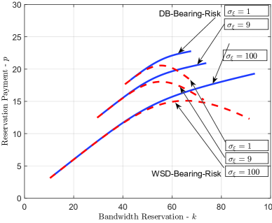
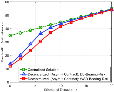
Figure 4: (a) Illustration of Optimal Contracts, (b) Contract-based Spectrum Reservations vs Scheduled Demand $\xi$. Here, $\sigma_{\xi}$ denotes the variance of scheduled demand $\xi$.

Then we compare the spectrum reservations under both contracts. By Proposition 2, both $k_{\textsc{(ii)}}^{*}(\xi)$ and $k_{\textsc{(i)}}^{*}(\xi)$ are increasing in $\xi$. By (21) and (32), we further have the following observation.

Lemma 3 (Contract-based spectrum reservation).

$$k_{\textsc{(ii)}}^{*}(\xi)\leq k_{\textsc{(i)}}^{*}(\xi)\leq k^{\circ}(\xi),\ \ \forall\xi\in[\underline{\xi},\bar{\xi}],$$

and $k_{\textsc{(ii)}}^{*}({\xi})=k_{\textsc{(i)}}^{*}(\xi)=k^{\circ}({\xi})$ only when $\xi=\bar{\xi}$.

That is, only when the realized scheduled demand $\xi$ reaches its maximum value (i.e., $\xi=\bar{\xi}$), the spectrum reservations under both optimal contracts are identical, and are equal the integrated optimal spectrum reservation. Under other values of $\xi$, the spectrum reservation in the contract $\Psi_{\textsc{(ii)}}^{*}$ (under WSD-bearing-risk) is smaller than that in the contract $\Psi_{\textsc{(i)}}^{*}$ (under DB-bearing-risk), which is further smaller than the integrated optimal spectrum reservation.

We illustrate the result of Lemma 3 in Figure 4.b. Intuitively, When the database bears the risk, it has an incentive to charge a high reservation fee in order to force the WSD to shoulder some of the potential cost. When the WSD bears the risk, however, the database has less incentive to charge a high reservation fee. Hence, for the same $\xi$, we find that $p_{\textsc{(i)}}^{*}(\xi)>p_{\textsc{(ii)}}^{*}(\xi)$. Combined with Proposition 1, we have $k_{\textsc{(ii)}}^{*}(\xi)<k_{\textsc{(i)}}^{*}(\xi)$.

VII Numerical Results

In this section, we provide numerical results to compare the performances of the proposed contract-based spectrum reservation mechanisms. Practically speaking, the database’s contract choice depends on many factors, among which the spectrum reservation decision and the resulting (expected) profit are the most important ones. Hence, we will present the expected profits (of the database, WSD, and the aggregated one) under different contracts associated with different risk-bearing schemes. Unless specified otherwise, we assume the following spectrum trading parameters: $r=1$, $s=0.8$, $w=0.5$, and $c=0.2$. We further assume that the scheduled demand $\xi$ follows the normal distribution, and the bursty demand $\varepsilon$ follows the chi-square distribution.

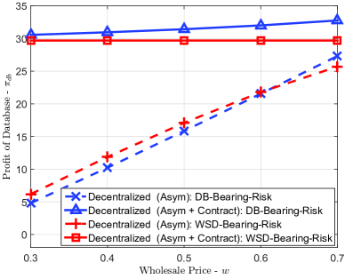
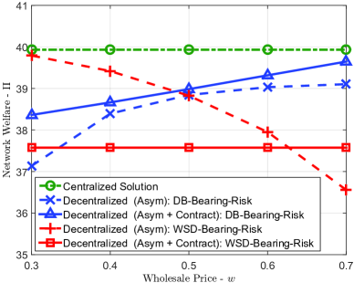
Figure 5: (a) Database Profit vs Wholesale Price, and (b) Network Profit vs Wholesale Price.

VII-A Profit vs Wholesale Price

Figure 5 illustrates (a) the database profit and (b) the network profit (aggregate profit) achieved in different spectrum reservation solutions (associated with information asymmetric under different wholesale prices $w$.) In this simulation, we assume that $\xi$ follows the normal distribution with mean $\mu_{\xi}=30$ and variance $\sigma_{\xi}^{2}=64$, and $\varepsilon$ follows the chi-square distribution with mean $\mu_{\varepsilon}=30$ and variance $\sigma_{\varepsilon}^{2}=60$.

From Figure 5.a, we have the following observations regarding the database profit.

• Under both risking bear-schemes, the contract-based spectrum reservation leads to a much higher profit for the database, compared to the reservation solution without information sharing.

• The database can achieve a higher profit with the optimal spectrum reservation contract under DB-bearing-risk (the blue triangle curve) than that under WSD-bearing-risk (the red square curve).

This is quite counter-intuitive. The reason is that the WSD is more risk-averse than the database.

From Figure 5.b, we have the following observations.

• Centralized Optimal Network Profit: The green circle curve denotes the optimal network profit achieved in the centralized reservation solution $k^{\circ}$ given in (3), which is independent of the wholesale price $w$, and serves as an upper-bound of the network profit under any other reservation solution.

• Network Profit under DB-Bear-Risk: The blue “x” (dash) curve and blue triangle (solid) curve denote the network profit achieved under DB-Bearing-Risk, without and with contract, respectively. Specifically, the former one is achieved from the reservation solution without information sharing, i.e., $k_{\textsc{(i)}}^{\textsc{asy}}$ given in (8). The latter one is achieved from the optimal spectrum reservation contract $\Psi_{\textsc{(i)}}^{*}$ given in Theorem 1. Obviously, information sharing based on the optimal spectrum reservation contract proposed in this paper improves the total network profit up to $5\%$.

• Network Profit under WSD-Bear-Risk: The red “$+$” (dash) curve and red square (solid) curve denote the network profit achieved under WSD-Bearing-Risk, with and without contract, respectively. Specifically, the former one is achieved from the reservation solution without information sharing, i.e., $k_{\textsc{(ii)}}^{\textsc{asy}}$ given in (12). The latter one is achieved from the optimal spectrum reservation contract $\Psi_{\textsc{(ii)}}^{*}$ given in Theorem 2. Different with the DB-Bearing-Risk scheme, we can see that only when the wholesale price $w$ is large (e.g., $w>0.62$ in this example), the performance under the optimal spectrum reservation contract is better than that without information sharing. This is because the purpose of contract under the WSD-bearing-risk is to reduce the double marginalization effect. Hence, the network profit under WSD-Bearing-Risk contract is independent of the wholesale price. However, as the objective of contract is maximizing the database profit, the database would charge an equivalent high “wholesale price” from the WSD. As shown by the Figure 5.b, such equivalent “wholesale price” lies between $0.6$ and $0.7$. This high equivalent high wholesale price decreases the performance of social welfare.

Our results provide the following important insight for a general reservation problem: it is not only individually better, but also socially better to leave the over-reservation risk to the less risk-averse decision maker.

VII-B Profit vs Scheduled Demand Variance

Figure 6 illustrates (a) the database profit and (b) the network profit achieved in different spectrum reservation solutions (associated with information asymmetry), under different scheduled demand variance $\sigma_{\xi}^{2}$. Notice that $\sigma_{\xi}^{2}$ reflects the degree of information asymmetry. That is, a higher $\sigma_{\xi}^{2}$ implies a larger variance of $\xi$, and thus a higher uncertainty of the database regarding $\xi$. In this simulation, we assume that $\xi$ follows the normal distribution with mean $\mu_{\xi}=30$ (and with different variances), and $\varepsilon$ follows the chi-square distribution with mean $\mu_{\varepsilon}=30$ and variance $\sigma_{\varepsilon}^{2}=60$.

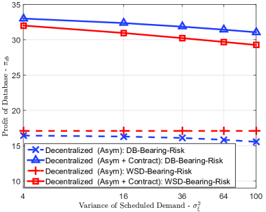
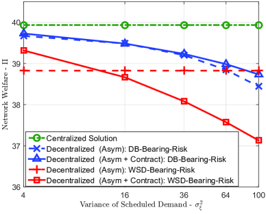
Figure 6: (a) Database Profit vs Scheduled Demand Variance, and (b) Network Profit vs Scheduled Demand Variance.

From Figure 6.a, we can further see that under both risk-bearing schemes, the optimal contracts ($\Psi_{\textsc{(i)}}^{*}$ and $\Psi_{\textsc{(ii)}}^{*}$) can greatly improve the database profit. Moreover, the database can achieve a slightly higher profit with the optimal contract $\Psi_{\textsc{(i)}}^{*}$ under DB-bearing-risk, than the optimal contract $\Psi_{\textsc{(ii)}}^{*}$ under WSD-bearing-risk.

Figure 6.b leads to a similar observation as Figure 5.b. Specifically, under DB-bearing-risk, the optimal contract $\Psi_{\textsc{(i)}}^{*}$ can always increase with the total network profit; while under WSD-bearing-risk, the optimal contract $\Psi_{\textsc{(ii)}}^{*}$ can only increase the total network profit when $\sigma_{\xi}^{2}$ is small (i.e., when the degree of information asymmetry is low). We can further see that the profits under both optimal contracts decrease with $\sigma_{\xi}^{2}$. This is because with a larger $\sigma_{\xi}^{2}$, the scheduled demand $\xi$ varies more dramatically. As the scheduled demand $\xi$ is the private information of the WSD, the larger variance of $\xi$ means that the database needs to pay a higher information rent to the WSDs.

VIII Conclusion

We propose a broker-based spectrum reservation market model for TV white space network, under stochastic demand and information asymmetry. To solve the problem, we propose a contract-based spectrum reservation framework, which ensures WSDs share their private information credibly. We analyze the incentive compatibility of contracts, and further derive the optimal contracts under different risk-bearing schemes. Our analysis and extensive simulations indicate that the optimal contract under DB-bearing-risk leads to a higher database profit and higher network profit than that under WSD-bearing-risk. As there is no large-scale commercializatin of TV white space network with detailed spectrum reservation scheme, our work can serve as a first step to give theoretical insights into the problem of risk-bearing between the database and the WSD, and promote the economic study of such a network.

In this work, we have focused on the TV white space network, where the primary users are the TV broadcasters. As the TV towers have fixed locations and TV programs have well planned schedules, the database has full information regarding the primary usage of TV spectrum ahead of time. This allows us to focus on the demand uncertainty from unlicensed users in this paper. On the other hand, the issue of primary usage uncertainly becomes much more important, if we consider the Licensed Shared Access (LSA) and Authorised Shared Access (ASA) models, where unlicensed users may access specific non-TV band (e.g., $3.5$ GHz band in the United States and $2.3$ GHz band in Europe). This is because these bands are used for ship- and air-borne radar systems which are critical to the operation of the national defense. Our model can be directly extended to analyze the LSA/ASA systems, if there is no penalty to the database and the WSD for not being able to serve all demands. However, when the expected payoffs of the database and the WSD depend on both the demand randomness and the available spectrum randomness, it would be much more challenging to obtain theoretical results by solving the contract design problem. We will consider the issue of two-sided uncertainty and the interaction among the licensee, the database, and the WSDs in our future work.

Appendix A Appendix

A-A Total Spectrum Reservation

In this section, we will show how the database determines the optimal aggregate reservation after knowing WSDs’ contract item choices.

A-A1 Aggregate Reservation under DB-Bearing-Risk

Under the DB-bearing-risk scheme, a WSD only purchases the spectrum that it actually needs in each access period, and hence the database can sell the over-reserved spectrum to other co-located WSDs in each access period.

Consider a set $\mathcal{N}$ of co-located WSDs. Suppose that in a particular reservation period, the scheduled demand of each WSD $n\in\mathcal{N}$ is $\xi_{n}$. By the incentive compatibility of the optimal contract $\Psi_{\textsc{(i)}}^{*}=\{\langle k_{\textsc{(i)}}^{*}(\xi),p_{\textsc{(i)}}^{*}(\xi)\rangle\}_{\forall\xi}$ (defined in Theorem 1), each WSD $n$ will choose the reservation amount $k_{\textsc{(i)}}^{*}(\xi_{n})$ intended for its demand type. Without the further optimization on the aggregate reservation, the database will simply reserve an amount $k_{\textsc{(i)}}^{*}(\xi_{n})$ for each WSD $n$, hence the total reservation is $K_{0}=\sum_{n\in\mathcal{N}}k_{\textsc{(i)}}^{*}(\xi_{n})$. Next we study how to further optimize the aggregate reservation for the database.

Let $\xi_{0}=\sum_{n\in\mathcal{N}}\xi_{n}$ denote the aggregated scheduled demand of all WSDs in $\mathcal{N}$, and let $\varepsilon_{0}=\sum_{n\in\mathcal{N}}\varepsilon_{n}$ denote the aggregated bursty demand of all WSDs in $\mathcal{N}$. Note that $\xi_{0}$ does not change during the whole reservation period, while $\varepsilon_{0}$ changes every access period. Moreover, the database can deduce the previous value of the scheduled demand $\xi_{n}$ of each WSD $n$ (hence the total scheduled demand $\xi_{0}$) from the WSDs’ selections. However, neither the database nor the WSDs can obtain the precise value of $\varepsilon_{0}$, as it changes every access period. Let $h(\varepsilon_{0})$ and $H(\varepsilon_{0})$ denote the p.d.f and c.d.f. of $\varepsilon_{0}$, respectively.

It is easy to see that when the realized total demand $D_{0}=\xi_{0}+\varepsilon_{0}$ is smaller than the total reservation $K_{0}$, the database can reduce the reservation cost by reducing the reservation amount. With a reduced aggregate reservation, on the other hand, the database may need to replenish the spectrum reservation (with a higher replenishment cost) when the realized total demand $D_{0}$ is larger than the aggregate reservation. Let $K_{\textsc{(i)}}$ denote that the reduced aggregate reservation of the database (for WSDs $\mathcal{N}$). Let $K_{0}=\sum_{n\in\mathcal{N}}k_{\textsc{(i)}}^{*}(\xi_{n})$ denote the total reservation requests of all WSDs, and we have $K_{\textsc{(i)}}\leq K_{0}$ as each WSD will not purchase an amount larger than its request.

The database profit depends on the actual realization of total demand $D_{0}$. Let $c$ be the database’s reservation cost, and let $c^{\textsc{ex}}>c$ be the replenishment cost. Then, we have, (a) when $D_{0}\leq K_{\textsc{(i)}}$, the database can reduce the reservation cost by $c\cdot(K_{0}-K_{\textsc{(i)}})$; (b) when $K_{\textsc{(i)}}\leq D_{0}\leq K_{0}$, the database needs to replenish a reservation amount $D_{0}-K_{\textsc{(i)}}$ to meet the requirements of WSDs, which will introduce a total replenishment cost of $c^{\textsc{ex}}\cdot(D_{0}-K_{\textsc{(i)}})$; (c) when $K_{0}\leq D_{0}$, the database needs to replenish a reservation amount $K_{0}-K_{\textsc{(i)}}$ to meet the requirements of WSDs, which will introduce a total replenishment cost of $c^{\textsc{ex}}\cdot(K_{0}-K_{\textsc{(i)}})$. Based on the above discussion, the expected increasing profit of the database is

$$\pi_{\textsc{db}}^{\textsc{a}}= \mathbb{E}_{\varepsilon_{0}}\bigg{[}c\cdot(K_{0}-K_{\textsc{(i)}})\cdot\text{Pr}(D_{0}\leq K_{\textsc{(i)}}\leq K_{0})$$ (35)

$$\qquad{}-c^{\textsc{ex}}\cdot(D_{0}-K_{\textsc{(i)}})\cdot\text{Pr}(K_{\textsc{(i)}}\leq D_{0}\leq K_{0})$$

$$\qquad{}-c^{\textsc{ex}}\cdot(K_{0}-K_{\textsc{(i)}})\cdot\text{Pr}(K_{\textsc{(i)}}\leq K_{0}\leq D_{0})\bigg{]}$$

The database’s optimal aggregate reservation $K_{\textsc{(i)}}^{*}$ that maximizes (35) satisfies

$$c^{\textsc{ex}}+c\cdot(K_{0}-K_{\textsc{(i)}}^{*})\cdot h(K_{\textsc{(i)}}^{*}-\xi_{0})$$ (36)

$$\qquad{}\quad{}-(c+c^{\textsc{ex}})\cdot H(K_{\textsc{(i)}}^{*}-\xi_{0})=0.$$

Obviously, $K_{\textsc{(i)}}^{*}$ is a function of $\xi_{0}$.

Figure 7 illustrates the database profit with and without aggregate reservation optimization under different numbers of WSDs. The blue-square and the red-circle curves denote the database profit with and without further optimization on the aggregate reservation, respectively. In this simulation, we assume that different WSDs’ scheduled demands $\xi_{n}$, $n\in\mathcal{N}$ are i.i.d., and different WSDs’ bursty demands $\varepsilon_{n}$, $n\in\mathcal{N}$ are also i.i.d. The scheduled demand $\xi_{n}$ of each WSD $n$ follows a normal distribution with mean $\mu_{\xi}=9$ and variance $\sigma_{\xi}^{2}=3$. The bursty demand $\varepsilon_{n}$ of each WSD $n$ follows a chi-square distribution with different values of the degrees of freedom.

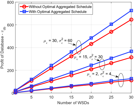
Figure 7: Database profit vs. numbers of WSDs, where $\mu_{\varepsilon}$ and $\sigma_{\varepsilon}^{2}$ denote the mean and variance of the bursty demand of each WSD $n$, respectively.

Figure 7 shows that with the further optimization, the database can increase its profit up to $12\%$. This benefit increases with the number of WSDs, as more WSDs submitting their spectrum reservation requirements, more freedom for the database to assign over-reserved spectrum of one WSD to other WSDs in need. As the mean $\mu_{\varepsilon}$ and variance $\sigma_{\varepsilon}^{2}$ of the bursty demand increase, the difference between the database profit with and without aggregated reservation schedule also increases.

A-A2 Aggregate Reservation under WSD-Bearing-Risk

Under the DB-bearing-risk scheme, a WSD purchases all the spectrum it requests in each access period, even if the realized demand is smaller than the requested reservation. Hence, the database cannot sell the over-reserved spectrum to other co-located WSDs in each access period. In this case, the database does not need to make the further optimization on the aggregate reservation. Namely, the database’s optimal aggregate reservation $K_{\textsc{(ii)}}^{*}$ is,

$$K_{\textsc{(ii)}}^{*}=\sum_{n\in\mathcal{N}}k_{\textsc{(ii)}}^{*}(\xi_{n}),$$ (37)

which is exactly the total requested reservation of all WSDs.

A-B Proof for Lemma 1

Proof.

Since $s>w>c$, we have $k^{\circ}$ is always larger than $k_{\textsc{(i)}}^{\textsc{sym}}$ and $k_{\textsc{(ii)}}^{\textsc{sym}}$. Note that $k_{\textsc{(i)}}^{\textsc{sym}}=\xi+{G^{-1}\Big{(}{(w-c)}/{w}\Big{)}}$ is monotonic increasing with wholesale price $w$ while $k_{\textsc{(ii)}}^{\textsc{sym}}=\xi+{G^{-1}\Big{(}{(s-w)}/{s}\Big{)}}$ decreases monotonically with $w$. We can easily get the conclusion. ∎

A-C Proof for Lemma 2

Proof.

Note that (6) and (11) show that the optimal bandwidth $k\geq\xi$ for any realized $\xi$. Hence, we can write the expected network profit in (2) with respect to $\xi$ as:

$$\mathbb{E}_{\xi}[\Pi]= (r-c)E_{\xi}[k]$$ (38)

$$-(r-s)(\mathbb{E}_{\xi}[k]-\mu_{\xi})-s\cdot\int_{0}^{\mathbb{E}_{\xi}[k]-\mu_{\xi}}G(u)\mathrm{d}u$$

where $\mu_{\xi}=\mathbb{E}[\xi]$ is the mean of the scheduled demand. Moreover, the first derivative with respect to expected bandwidth $\mathbb{E}_{\xi}[k]$ is:

$$\frac{\partial{\mathbb{E}_{\xi}[\Pi]}}{\partial{\mathbb{E}_{\xi}[k]}} =(s-c)-s\cdot G(\mathbb{E}_{\xi}[k]-\mu_{\xi})$$ (39)

and the second derivative is $-s\cdot g(\mathbb{E}_{\xi}[K]-\mu_{\xi})\leq 0$. Hence, the maximum solution of (38) is $\mathbb{E}_{\xi}[k^{\circ}]$ and the network profit increases with $\mathbb{E}_{\xi}[k]$ when $\mathbb{E}_{\xi}[k]<\mathbb{E}_{\xi}[k]$. By applying Lemma 1, we can get the conclusion. ∎

A-D Proof for Proposition 1

Proof.

We prove it by contradiction. $\leftarrow$: When $\xi=\xi_{1}$, the following IC constraint must be satisfied:

$$(s-w)\mathbb{E}_{\varepsilon}\big{[}\min\big{\{}{\varepsilon},(k(\xi_{2})-\xi_{1})^{+}\big{\}}\big{]}$$ (40)

$$~{}~{}-(s-w)\mathbb{E}_{\varepsilon}\big{[}\min\big{\{}{\varepsilon},(k({\xi_{1}})-\xi_{1})\big{\}}\big{]}\geq p(\xi_{2})-p(\xi_{1})$$

from which we can find that if $p(\xi_{1})>p(\xi_{2})$, then $k(\xi_{1})>k(\xi_{2})$. For otherwise, the IC cannot be satisfied. $\rightarrow$: We first differentiate (19) with respect to $\xi$ and get:

$$\frac{\mathrm{d}{p(\xi)}}{\mathrm{d}{\xi}}=(s-w)\cdot[1-G(k(\xi)-\xi)]\cdot\frac{\mathrm{d}{k(\xi)}}{\mathrm{d}{\xi}}$$ (41)

Then we can conclude that if $K(\xi_{1})>K(\xi_{2})$, then $P(\xi_{1})>P(\xi_{2})$ ∎

A-E Proof for Proposition 2

Proof.

We prove it by contradiction. Note that:

$$\frac{\partial^{2}{\pi_{\textsc{ms}}(k,p,\xi)}}{\partial{k}\partial{\xi}}=(s-w)g\big{(}k-\xi\big{)} >0,\mathrm{~{}~{}and~{}~{}}$$ (42)

$$\frac{\partial^{2}{\pi_{\textsc{ms}}(k,p,\xi)}}{\partial{k}^{2}}=-(s-w)g\big{(}k-\xi\big{)}<0.$$ (43)

Hence, for any $\xi_{1}>\xi_{2}$, if $k(\xi_{1})<k(\xi_{2})$. That we have:

$$0 =\left.\frac{\partial{\pi_{\textsc{ms}}\left(k,p,\xi_{1}\right)}}{\partial{k}}\right|_{k=k(\xi_{1})}$$

$$>\left.\frac{\partial{\pi_{\textsc{ms}}\left(k,p,\xi_{1}\right)}}{\partial{k}}\right|_{k=k(\xi_{2})}$$

$$>\left.\frac{\partial{\pi_{\textsc{ms}}\left(k,p,\xi_{2}\right)}}{\partial{k}}\right|_{k=k(\xi_{2})},$$

where the equality is because of IC and the inequalities are because of the sign of the second-order derivatives. But this contradicts the optimality of $k\left(\xi_{2}\right)$. ∎

A-F Proof for Proposition 3

Proof.

The IC constraint implies that $\pi_{\textsc{ms}}({\xi})=\max_{\hat{\xi}}\pi_{\textsc{ms}}\big{(}k(\hat{\xi}),p(\hat{\xi}),\xi\big{)}$. The envelope theorem further shows that:

$$\frac{\mathrm{d}{\pi_{\textsc{ms}}}(\xi)}{\mathrm{d}{\xi}} =\left.\frac{\partial{\pi_{\textsc{ms}}(k({\hat{\xi}}),p(\hat{\xi}),\xi_{i})}}{\partial{\xi}}\right|_{\hat{\xi}=\xi}$$ (44)

$$=(r-s)+(s-w)G\big{(}k({\xi})-\xi\big{)}>0.$$

Then we have $\pi_{\textsc{ms}}(\xi)$ is increasing in $\xi$. ∎

A-G Proof for Proposition 4

Proof.

By using IC constraint and the envelope theorem, we have:

$$\frac{\mathrm{d}{\pi_{\textsc{ms}}}(\xi)}{\mathrm{d}{\xi}} =\left.\frac{\partial{\pi_{\textsc{ms}}(k({\hat{\xi}}),p(\hat{\xi}),\xi_{i})}}{\partial{\xi}}\right|_{\hat{\xi}=\xi}$$ (45)

$$=(r-s)+(s-w)G\big{(}k({\xi})-\xi\big{)}.$$

By integrating both sides, we get the Proposition 4. ∎

A-H Proof for Proposition 5

Proof.

We only have to show that these three conditions imply IC and IR. Noted that (19), $\pi_{\textsc{ms}}(\xi)$ is obtained by Lemma (4). We therefore have:

$$\pi_{\textsc{ms}}\big{(}k(\hat{\xi}),p(\hat{\xi}),\xi\big{)}$$

$$\quad{}={\int_{\underline{\xi}}^{\xi}}\frac{\partial{\pi_{\textsc{ms}}\big{(}k(\hat{\xi}),p(\hat{\xi}),x\big{)}}}{\partial{x}}\mathrm{d}{x}+\pi_{\textsc{ms}}\big{(}k(\hat{\xi}),p(\hat{\xi}),\underline{\xi}\big{)}$$

$$\quad{}=\pi_{\textsc{ms}}\big{(}k(\hat{\xi}),p(\hat{\xi}),\hat{\xi}\big{)}$$

$$\qquad{}+{\int_{\hat{\xi}}^{\xi}}\big{[}(r-s)+(s-w)\cdot G\big{(}k(\xi)-x\big{)}\big{]}\mathrm{d}{x}$$

$$\quad{}=\pi_{\textsc{ms}}\big{(}k(\xi),p(\xi),\xi\big{)}$$

$$\qquad{}+{\int_{\hat{\xi}}^{\xi}}(s-w)\big{[}G\big{(}k(\hat{\xi})-x\big{)}-G\big{(}k(x)-x\big{)}\big{]}\mathrm{d}{x}$$

If $\xi>\hat{\xi}$, then the above equation is non-positive (because both $k$ and $G$ are increasing) and hence $\pi_{\textsc{ms}}\big{(}k(\xi),p(\xi),\xi\big{)}\geq\pi_{\textsc{ms}}\big{(}k({\hat{\xi}}),p(\hat{\xi}),\xi\big{)}$. This inequality also holds for $\xi<\hat{\xi}$ by a similar argument. Therefore, the two condition imply IC.

Evaluate $\pi_{\textsc{ms}}(\xi)$ at $\underline{\xi}$ and using (6), we can get IR immediately. ∎

A-I Proof for Proposition 6

Proof.

Let $i=1,2$ and define ${\hat{\xi}}_{i}^{*}=\arg\max_{\hat{\xi}}\pi_{\textsc{ms}}\big{(}k(\hat{\xi}),p(\hat{\xi}),\xi_{i}\big{)}$ We therefore have $\pi_{\textsc{ms}}\big{(}k({\hat{\xi}}_{1}^{*}),p({\hat{\xi}}_{1}^{*}),\xi_{2}\big{)}\leq\pi_{\textsc{ms}}\big{(}k({\hat{\xi}}_{2}^{*}),p({\hat{\xi}}_{2}^{*}),\xi_{2}\big{)}$. Noted that:

$$\frac{\partial{\pi_{\textsc{ms}}\big{(}k({\hat{\xi}}),p(\hat{\xi}),\xi\big{)}}}{\partial{\xi}} =(r-s)+(s-w)G\big{(}k(\hat{\xi})-\xi\big{)}$$

$$\geq 0.$$

Hence, for any $\xi_{1}<\xi_{2}$, We have $\pi_{\textsc{ms}}\big{(}k({\hat{\xi}}_{1}^{*}),p({\hat{\xi}}_{1}^{*}),\xi_{1}\big{)}\leq\pi_{\textsc{ms}}\big{(}k({\hat{\xi}}_{1}^{*}),p({\hat{\xi}}_{1}^{*}),\xi_{2}\big{)}$. By using the IC constraint, we have ${\hat{\xi}}_{i}^{*}=\xi_{i}$, and therefore $\pi_{\textsc{ms}}\big{(}k(\xi_{1}),p(\xi_{1}),\xi_{1}\big{)}\leq\pi_{\textsc{ms}}\big{(}k(\xi_{2}),p(\xi_{2}),\xi_{2}\big{)}$. Hence IR only needs to be satisfied at $\xi=\underline{\xi}$ and the other participation constraints for $\xi>\underline{\xi}$ are redundant. Hence, we get (6). ∎

A-J Proof for Theorem 1

This Theorem can be simply proved by using Proposition 5 and Proposition 6. Here we jus show that the optimal point of $\phi_{\textsc{(i)}}(k(\xi),\xi)$ is unique by proving $\phi_{\textsc{(i)}}(k(\xi),\xi)$ is unimodal.

Proof.

We let $z(\xi)=k(\xi)-\xi$, then we rewrite $\phi_{\textsc{(i)}}(k(\xi),\xi)$ as $\phi_{\textsc{(i)}}(z(\xi))$ and get

$$\frac{\partial{\phi_{\textsc{(i)}}(z)}}{\partial{z}}= s\cdot[1-G(z)]-c-\frac{1-F(\xi)}{f(\xi)}(s-w)g(z).$$ (46)

To prove that $\phi_{\textsc{(i)}}(z)$ is unimodal, it suffices to show that ${\partial{\phi_{\textsc{(i)}}(z)}}/{\partial{z}}$ changes the sign once. Note that $\varepsilon$ follows chi-square distribution with support $[0,+\infty)$. Then we have $\lim_{z\rightarrow 0}{\partial{\phi_{\textsc{(i)}}(z)}}/{\partial{z}}=s-c>0$,and $\lim_{z\rightarrow+\infty}{\partial{\phi_{\textsc{(i)}}(z)}}/{\partial{z}}=-c<0$. Then we consider the second order derivative of $\phi_{\textsc{(i)}}(z)$ with respect to $z$ and we have

$$\frac{\partial^{2}{\phi_{\textsc{(i)}}(z)}}{\partial{z^{2}}} =-s\cdot g(z)-\frac{1-F(\xi)}{f(\xi)}(s-w)g^{{}^{\prime}}(z)$$ (47)

$$=\frac{z^{\frac{n}{2}-2}e^{-\frac{z}{2}}}{\Gamma(\frac{n}{2})2^{\frac{n}{2}}}\left[\frac{A(\xi)-2}{2}z-A(\xi)\left(\frac{n}{2}-1\right)\right]$$

where $A(\xi)={\left((1-F(\xi))(s-w)\right)}/{(s\cdot f(\xi))}$ and $n$ is the freedom of chi-square distribution. Note that $\lim_{z\rightarrow+\infty}{\partial^{2}{\phi_{\textsc{(i)}}(z)}}/{\partial{z^{2}}}<0$, and case 1: $\frac{A-2}{2}<0$, then ${\partial^{2}{\phi_{\textsc{(i)}}(z)}}/{\partial{z^{2}}}<0$, and ${\partial{\phi_{\textsc{(i)}}(z)}}/{\partial{z}}$ changes the sign once; case 2: $\frac{A-2}{2}>0$, then the value of ${\partial^{2}{\phi_{\textsc{(i)}}(z)}}/{\partial{z^{2}}}$ is first negative, then becomes positive. However, as ${\partial^{2}{\phi_{\textsc{(i)}}(z)}}/{\partial{z^{2}}}$ is the linear function of $z$, then ${\partial{\phi_{\textsc{(i)}}(z)}}/{\partial{z}}$ only changes the sign once.

If $\varepsilon$ follows from normal distribution with mean $\mu$ and standard variance $\sigma$, then $\phi_{\textsc{(i)}}(z)$ is also unimodal as long as $G(x)\rightarrow 0$ when $x<0$. In such case, $\lim_{z\rightarrow 0}{\partial{\phi_{\textsc{(i)}}(z)}}/{\partial{z}}=s-c>0$, and $\lim_{z\rightarrow+\infty}{\partial{\phi_{\textsc{(i)}}(z)}}/{\partial{z}}=-c<0$. And

$$\frac{\partial^{2}{\phi_{\textsc{(i)}}(z)}}{\partial{z^{2}}} =-s\cdot g(z)-\frac{1-F(\xi)}{f(\xi)}(s-w)g^{{}^{\prime}}(z)$$

$$=\frac{1-F(\xi)}{f(\xi)}\frac{s-w}{s}\frac{1}{\sigma\sqrt{2\pi}}e^{-\frac{(z-\mu)^{2}}{2\sigma^{2}}}\left[\frac{z}{\sigma^{2}}-\frac{\mu}{\sigma^{2}}-1\right]$$

The above equation shows that the value of ${\partial^{2}{\phi_{\textsc{(i)}}(z)}}/{\partial{z^{2}}}$ first is negative, then become positive. However, as ${\partial^{2}{\phi_{\textsc{(i)}}(z)}}/{\partial{z^{2}}}$ is the linear function of $z$, then ${\partial{\phi_{\textsc{(i)}}(z)}}/{\partial{z}}$ only changes the sign once. ∎

A-K Proof for Proposition 7

Proof.

By using IC constraint and the envelope theorem, we have:

$$\frac{\mathrm{d}{\pi_{\textsc{ms}}}(\xi)}{\mathrm{d}{\xi}} =\left.\frac{\partial{\pi_{\textsc{ms}}(k({\hat{\xi}}),p(\hat{\xi}),\xi_{i})}}{\partial{\xi}}\right|_{\hat{\xi}=\xi}$$ (48)

$$=(r-s)+s\cdot G\big{(}k({\xi})-\xi\big{)}.$$

By integrating both sides, we get the Proposition 7. ∎

A-L Proof for Theorem 2

This Theorem can be simply proved by using Proposition 5 and Proposition 6. Here we jus show that the optimal point of $\phi_{\textsc{(ii)}}(k(\xi),\xi)$ is unique by proving $\phi_{\textsc{(ii)}}(k(\xi),\xi)$ is unimodal.

Proof.

We let $z(\xi)=k(\xi)-\xi$, then we rewrite $\phi_{\textsc{(ii)}}(k(\xi),\xi)$ as $\phi_{\textsc{(ii)}}(z(\xi))$ and get

$$\frac{\partial{\phi_{\textsc{(ii)}}(z)}}{\partial{z}}= s\cdot[1-G(z)]-c-\frac{1-F(\xi)}{f(\xi)}\cdot s\cdot g(z).$$ (49)

To prove that $\phi_{\textsc{(ii)}}(z)$ is unimodal, it suffices to show that ${\partial{\phi_{\textsc{(ii)}}(z)}}/{\partial{z}}$ changes the sign once. Note that $\varepsilon$ follows chi-square distribution with support $[0,+\infty)$. Then we have $\lim_{z\rightarrow 0}{\partial{\phi_{\textsc{(ii)}}(z)}}/{\partial{z}}=s-c>0$,and $\lim_{z\rightarrow+\infty}{\partial{\phi_{\textsc{(ii)}}(z)}}/{\partial{z}}=-c<0$. Then we consider the second order derivative of $\phi_{\textsc{(ii)}}(z)$ with respect to $z$ and we have

$$\frac{\partial^{2}{\phi_{\textsc{(ii)}}(z)}}{\partial{z^{2}}} =-s\cdot g(z)-\frac{1-F(\xi)}{f(\xi)}\cdot s\cdot g^{{}^{\prime}}(z)$$ (50)

$$=\frac{z^{\frac{n}{2}-2}e^{-\frac{z}{2}}}{\Gamma(\frac{n}{2})2^{\frac{n}{2}}}\left[\frac{A(\xi)-2}{2}z-A(\xi)\left(\frac{n}{2}-1\right)\right]$$

where $A(\xi)={\left((1-F(\xi))\cdot s\right)}/{(s\cdot f(\xi))}$ and $n$ is the freedom of chi-square distribution. Note that $\lim_{z\rightarrow+\infty}{\partial^{2}{\phi_{\textsc{(ii)}}(z)}}/{\partial{z^{2}}}<0$, and case 1: $\frac{A-2}{2}<0$, then ${\partial^{2}{\phi_{\textsc{(ii)}}(z)}}/{\partial{z^{2}}}<0$, and ${\partial{\phi_{\textsc{(ii)}}(z)}}/{\partial{z}}$ changes the sign once; case 2: $\frac{A-2}{2}>0$, then the value of ${\partial^{2}{\phi_{\textsc{(ii)}}(z)}}/{\partial{z^{2}}}$ is first negative, then becomes positive. However, as ${\partial^{2}{\phi_{\textsc{(ii)}}(z)}}/{\partial{z^{2}}}$ is the linear function of $z$, then ${\partial{\phi_{\textsc{(ii)}}(z)}}/{\partial{z}}$ only changes the sign once.

If $\varepsilon$ follows from normal distribution with mean $\mu$ and standard variance $\sigma$, then $\phi_{\textsc{(ii)}}(z)$ is also unimodal as long as $G(x)\rightarrow 0$ when $x<0$. In such case, $\lim_{z\rightarrow 0}{\partial{\phi_{\textsc{(ii)}}(z)}}/{\partial{z}}=s-c>0$, and $\lim_{z\rightarrow+\infty}{\partial{\phi_{\textsc{(i)}}(z)}}/{\partial{z}}=-c<0$. And

$$\frac{\partial^{2}{\phi_{\textsc{(ii)}}(z)}}{\partial{z^{2}}} =-s\cdot g(z)-\frac{1-F(\xi)}{f(\xi)}\cdot s\cdot g^{{}^{\prime}}(z)$$

$$=\frac{1-F(\xi)}{f(\xi)}\frac{s-w}{s}\frac{1}{\sigma\sqrt{2\pi}}e^{-\frac{(z-\mu)^{2}}{2\sigma^{2}}}\left[\frac{z}{\sigma^{2}}-\frac{\mu}{\sigma^{2}}-1\right]$$

The above equation shows that the value of ${\partial^{2}{\phi_{\textsc{(ii)}}(z)}}/{\partial{z^{2}}}$ first is negative, then become positive. However, as ${\partial^{2}{\phi_{\textsc{(ii)}}(z)}}/{\partial{z^{2}}}$ is the linear function of $z$, then ${\partial{\phi_{\textsc{(ii)}}(z)}}/{\partial{z}}$ only changes the sign once. ∎

A-M Proof for Lemma 3

Proof.

By comparing (21) and (32), we can easily get the conclusion. ∎

References

- [1] Y. Luo, L. Gao, and J. Huang, “Spectrum broker by geo-location database,” in IEEE GLOBECOM, 2012, pp. 5427-5432.
- [2] FCC 12-36, Third Memorandum Opinion and Order, USA, Federal Communications Commission, 2012.
- [3] Ofcom, Technical Report 08-260, “Implementing TV white spaces,” London, U.k., Feb. 2015.
- [4] S. Jones and T. Phillips, “Initial Evaluation of the Performance of Prototype Tv-Band White Space Devices,” Federal Communication Commission, Tech. Rep., 2007.
- [5] IEEE, “Ieee 802.22 working group on wireless regional area networks,” [online] http://www.ieee802.org/22/.
- [6] CEPT-ECC, Tech. Rep., “Ecc report 185: Further definition of technical and operational requirements for the operation of the operation of white space devices in the band 470-790 Mhz,” January 2013.
- [7] ETSI, Tech. Rep., “ETSI harmonized European standard for white spaces devies V 1.1.1,” April 2014.
- [8] H. Bogucka, M. Parzy, P. Marques, J. Mwangoka, and T. Forde, “Secondary spectrum trading in TV white spaces,” IEEE Communications Magazine, vol. 50, no. 11, pp. 121–129, November 2012.
- [9] G. P. Cachon and M. A. Lariviere, “Contracting to assure supply: How to share demand forecasts in a supply chain,” Management Science, vol. 47, no. 5, pp. 629–646, 2001.
- [10] Ö. Özer and W. Wei, “Strategic commitments for an optimal capacity decision under asymmetric forecast information,” Management Science, vol. 52, no. 8, pp. 1238–1257, 2006.
- [11] D. Niyato and E. Hossain, “Spectrum trading in cognitive radio networks: A market-equilibrium-based approach,” IEEE Wireless Communications, vol. 15, no. 6, pp. 71–80, December 2008.
- [12] X. Chen and J. Huang, “Game theoretic analysis of distributed spectrum sharing with database,” in IEEE ICDCS, 2012, pp. 255-264.
- [13] X. Feng, Q. Zhang, and J. Zhang, “Hybrid pricing for TV white space database,” in IEEE INFOCOM, 2013, pp. 1995-2003.
- [14] Y. Luo, L. Gao, and J. Huang, “Price and inventory competition in oligopoly TV white space markets,” IEEE Journal on Selected Areas in Communications, vol. 33, no. 5, pp. 1002–1013, May 2015.
- [15] Y. Luo, L. Gao, and J. Huang, “Trade Information, Not Spectrum: A Novel TV White Space Information Market Model”, IEEE WiOpt, 2014, pp. 405-412.
- [16] Y. Luo, L. Gao, and J. Huang, “Information Market for TV White Space”, IEEE INFOCOM Workshop on SDP, 2014.
- [17] Y. Luo, L. Gao, and J. Huang, “MINE GOLD to Deliver Green Cognitive Communications,” IEEE Journal on Selected Areas in Communications, vol. PP, no. 99, 2015.
- [18] Y. Luo, L. Gao, and J. Huang, “Business Modeling for TV White Space Networks”, IEEE Commun. Mag., vol. 53, no. 5, pp. 82-88, May 2015.
- [19] Y. Luo, L. Gao, and J. Huang, “HySIM: A Hybrid Spectrum and Information Market for TV White Space Networks”, IEEE INFOCOM, 2015, pp. 604-609.
- [20] L. Gao, X. Wang, Y. Xu, and Q. Zhang, “Spectrum trading in cognitive radio networks: A contract-theoretic modeling approach,” IEEE Journal on Selected Areas in Communications, vol. 29, no. 4, pp. 843–855, 2011.
- [21] L. Duan, L. Gao, and J. Huang, “Cooperative spectrum sharing: a contract-based approach,” IEEE Transactions on Mobile Computing, vol. 13, no. 1, pp. 174–187, 2014.
- [22] S. P. Sheng and M. Liu, “Profit incentive in a secondary spectrum market: A contract design approach,” in IEEE INFOCOM, 2013, pp. 836-844.
- [23] D. Niyato, E. Hossain, and Z. Han, “Dynamics of multiple-seller and multiple-buyer spectrum trading in cognitive radio networks: A game-theoretic modeling approach,” IEEE Transactions on Mobile Computing, vol. 8, no. 8, pp. 1009–1022, 2009.
- [24] A. Goldsmith, Wireless communications, Cambridge, U.K., Cambridge Univ. Press, 2005.
- [25] Y. Luo, L. Gao, and J. Huang, Tech. Report, online at http://jianwei.ie.cuhk.edu.hk/publication/WSN-Contract.pdf