Cosmic Rays Propagation with HelMod: Difference between forward-in-time and backward-in-time approaches

Abstract:

The cosmic rays modulation inside the heliosphere is well described by a transport equation introduced by Parker in 1965. To solve this equation several approaches were followed in the past. Recently the Monte Carlo approach becomes widely used in force of his advantages with respect to other numerical methods. In the Monte Carlo approach, the transport equation is associated to a fully equivalent set of Stochastic Differential Equations. This set is used to describe the stochastic path of a quasi-particle from a source, e.g., the interstellar medium, to a specific target, e.g., a detector at Earth. In this work, we present both the Forward-in-Time and Backward-in-Time Monte Carlo solutions. We present an implementation of both algorithms in the framework of HelMod Code showing that the difference between the two approach is below 5% that can be quoted as the systematic uncertain of the Method itself.

1 Introduction

Galactic Cosmic Rays (GCRs), entering into the heliosphere, experience of the so-called Solar Modulation: a reduction in the absolute flux, at energies $\lesssim 50$ GeV, with respect to the local interstellar spectrum (LIS). Particles propagating from the heliosphere boundary, located at $\sim 100$ AU, down to the Earth orbit have to pass through an expanding plasma emitted from the Sun (i.e. the Solar Wind). The small scale irregularities of the Sun magnetic field, carried out within the Solar Wind, causes a diffusion process of GCRs passing through the interplanetary medium. The interplanetary conditions vary as a function of the solar cycle, that is approximately 22 years, consequently the intensity of the solar modulation is related to this cycle. In general, particle propagation in the Heliosphere can be described using the well-known equation developed by Parker [1], based on a Fokker-Planck like Equation (FPE). The Parker’s equation was initially solved using the so called “Force Field” approach [2, 3, 4]. In this quasi-analytical solution the whole diffusion/convection process can be described using a single parameter, i.e. the “modulation potential”. Although this approximation is not able to reproduce all the physical processes in the heliosphere (see e.g. discussion in [5]), due to its simplicity it remains the reference method for experimental treatment of Solar Modulation. Numerical methods, e.g. Crank-Nicholson or finite difference method (see e.g.[6, 7]), were used to solve the Parker’s equation allowing to study in more detail the physics of the heliosphere. The Heliosphere Modulation Model (HelMod) [8, 9] implemented a new class of numerical methods, using a Monte Carlo technique. This is based on the mathematic equivalence between FPE and a set of Stochastic Differential Equation (SDEs) (see, e.g. Chapter 1.6-1.7 of [10]). As many authors underline, see e.g. [11, 12, 13, 14, 15, 16, 8, 17], this approach allows for more flexibility in model implementation, more stability of numerical results and to explore physical results that are hard to handle with “classical” numerical methods or even not possible in the simple Force Field approach (see e.g.[18, 9, 19]). In this work, we present two Monte Carlo solutions for the FPE applied on the problem of particle propagation in the heliosphere. The two solutions are obtained solving the FPE forward-in-time and backward-in-time.

2 Monte Carlo Method for HelMod

The galactic cosmic rays transport equation was originally proposed by Parker in his fundamental work [1, 20, 21, 8]. This transport equation is a Fokker-Plank like equation that describes the modulation of Cosmic Rays by means of the so-called omni-directional distribution function $f(\vec{x},p)$ (see e.g. [6, 13, 16]) :

$$\frac{\partial f}{\partial t}=-\nabla\cdot(f\vec{V})+\nabla\cdot\left[\tilde{K}\cdot\nabla f\right]+\frac{(\nabla\cdot\vec{V})}{3p^{2}}\frac{\partial}{\partial p}\left(p^{3}f\right),$$ (1)

where $p$ is particle momentum, $\vec{x}$ is the 3D-spatial position in Cartesian coordinates, $\vec{V}=\vec{V}_{sw}+\vec{V}_{drift}$, $\vec{V}_{sw}$ is the solar wind velocity, $\vec{V}_{drift}$ is the particle magnetic drift velocity and $\tilde{K}$ is the diffusion tensor. The differential intensity $J$ is related to $f$ as $J=p^{2}f$. For sake of clarity, in this work, we treat the stochastic solutions of simple one dimensional Parker’s equation in spherical coordinates. This allow us to focus directly on the numerical methods itself without adding to formulas the complexity of a more realistic treatment of the Heliosphere (see, e.g., [9] for a 2D forward-in-time solution of Parker’s equation using HelMod). In this approximation the diffusion tensor $\tilde{K}$ was simplified to be a scalar $\kappa_{diff}$ and all relevant description in the model (such as, e.g., the magnetic field and the solar wind) are spherically symmetric. Parker’s equation can be thus simplified as follows:

$$\frac{\partial f}{\partial t} = \frac{1}{r^{2}}\frac{\partial}{\partial r}\left(r^{2}\kappa_{diff}\frac{\partial}{\partial r}f\right)-\frac{1}{r^{2}}\frac{\partial r^{2}V_{sw}f}{\partial r}+\frac{1}{3}\left(\frac{1}{r^{2}}\frac{\partial r^{2}V_{sw}}{\partial r}\right)\frac{1}{p^{2}}\frac{\partial}{\partial p}(p^{3}f).$$ (2)

Since the magnetic field is assumed to be spherically symmetric, the magnetic drift velocity in radial direction is equal to zero. The Solar Wind ($V_{sw}$) is taken to be constant, radially directed and equal to $400$ km s^-1. The heliosphere in all approaches presented in this article is spherical with radius 100 AU and does not have Heliosheath or any other structure (Termination Shock, Heliopause, Bow Shock). In our Monte Carlo simulations we set an inner reflecting boundary at 0.3 AU.

With the Monte Carlo approach used in HelMod, the solution can be evaluated computing the SDE forward-in-time and backward-in-time. In forward-in-time approach quasi-particles were traced in the heliosphere from the Heliosphere boundary down to the inner Heliosphere. In backward-in-time approach the numerical process starts from the target, i.e. the Earth Orbit; quasi-particle objects are traced backward in time till the heliosphere boundary. In Ref. [16], authors underline that a pseudo-particle is not a real particle nor a test particle; these are points in phase space that have the tendency to follow field lines according to SDEs, but they do not in general follow them rigorously owing to the random Wiener process present in the equation (see, e.g.,  [16]).

In term of differential operators, formally the backward-in-time formulation is described by the adjoint operator of the forward-in-time [22]. This leads to the conclusion that, from the mathematically point of view, the two approaches describe the same process. However, in the knowledge of authors, in literature there is no contribution with direct quantitative comparison of spectra inside the heliosphere in order to have an estimation of a systematic error due to the numerical methods it self.

2.1 Forward-in-time

The forward-in-time evolution of the transition density function $Q(s,y;t,x)$, from a phase-space point $y$ at time $s$ to a new position $(t,x)$, can be written as the follow FPE (see Equation 1.7.14 of [10], Equation 8 of [14], Equation 7 of [16] and Equation 13 of [22]):

$$\frac{\partial Q}{\partial t}=-\sum_{i}\frac{\partial}{\partial x_{i}}[A_{F,i}(t,x)Q]+\frac{1}{2}\sum_{i,j}\frac{\partial^{2}}{\partial x_{i}\partial x_{j}}[C_{F,ij}(t,x)Q]-L_{F}(t,x)Q+S$$ (3)

where $A_{F,i}$ is the advective term for i-th coordinates (e.g. convection due to Solar Wind and Magnetic Drift), $C_{F,ij}$ is the diffusion tensor, $L_{F}$ is a bounded function that “removes” (or “adds”) particles during the propagation (e.g. fragmentation, radioactive decay, see e.g. [23], Section 17.2.1 of [24]) and finally $S$ represent a “source” of particles (e.g. Jovian Electrons, see [17]). This equation gives the forward-in-time evolution with respect to the final state $(t,x)$. In terms of SDEs, the evolution of the stochastic process can be described by (see e.g. Sections 4.3.2-4.3.5 of [25] and Appendix A.13.1 of [24]):

$$dx_{i}(t)=A_{F,i}dt+B_{F,i,j}dW_{j}(t),$$ (4)

where $\tilde{C}_{F}=\tilde{B}_{F}\tilde{B}_{F}^{T}$, $d\vec{W}$ represents the increments of a standard Wiener process that can be represented as an independent random variable of the form $\sqrt{dt}N(0,1)$ and, finally, $N(0,1)$ denotes a normally distributed random variable with zero mean value and unit variance (See e.g., Appendix A of [14] and Section 2 of [26]). In term of stochastic propagation, the linear part $L_{F}$ is an additional parameter that allows the stochastic process to be created at an exponential rate as function of time [14].

The Set of SDEs for the considered Parker’s Equation can be obtained rewriting Eq. 2 in the form of Eq. 3 (this can be done applying the substitution $F=r^{2}f$ as indicated, e.g., in Refs. [13, 27, 16, 8]). Then, using the equivalence with Eq. 4 the discrete forward-in-time SDEs are the following (hereafter, we will refer to this as F-p from Forward SDE with momentum p):

$$\Delta r = \left(\frac{2\kappa_{diff}}{r}+V_{sw}\right)\Delta t+N(0,1)\sqrt{(2\kappa_{diff}\Delta t)}$$ (5)

$$\Delta p = -\frac{2V_{sw}p}{3r}\Delta t$$ (6)

$$L_{F} = -\frac{4V_{sw}}{3r}$$ (7)

In the Monte Carlo Forward-in-time approach the stochastic path described by Eqs. 5-7 is followed by quasi-particle objects injected at heliosphere boundary. The initial momentum distribution is chosen in order to sample the Local Interstellar Spectrum (LIS) distribution at heliosphere border. According to the sampling method, to each quasi-particle is associated a weight $w_{0}$ that reflect the LIS distribution probability. This weight is modified each $j$-th step during the propagation (from generation $j=0$ to registration $j=k$) in order to account for the Linear term $L$ of Eq. 3 (see Equation 22 in [22]):

$$W=w_{0}\exp(-\sum_{j=0}^{k}L_{F,j}\Delta t)$$ (8)

When a quasi-particle pass through a selected position, momentum and weight, i.e., the one computed with Eq. 8, are registered. The modulated spectrum is obtained using a proper normalization scaling factor on the binned registered distribution. This is equivalent to apply the algorithm 17.2 of [24].

2.2 Backward-in-time

The Backward-in-time evolution of a FPE is described by the Kolmogorov backward equation (see Equation 1.7.15 in Ref. [10]). This equation gives the backward evolution of the associated transition density function with respect to the initial state $(s,y)$ (se e.g. Equation 13 of [14], Equation A2 of [17], Equation 14 of [22]):

$$\frac{\partial Q}{\partial s}=+\sum_{i}A_{B,i}(s,y)\frac{\partial Q}{\partial y_{i}}+\frac{1}{2}\sum_{i,j}C_{B,ij}(s,y)\frac{\partial^{2}Q}{\partial y_{i}\partial y_{j}}-L_{B}Q+S$$ (9)

The meaning of the terms in Eq. 9 are the same of Eq. 3. These are here presented with different subscript since the diffusion and advective coefficients of forward and backward approach are the same only for the special case of constant value [22]. Thus, Eq. 2 is associated with the following set of SDE for the backward-in-time evolution (hereafter we will refer to this as B-p from Backward SDE with momentum p):

$$\Delta r = \left(\frac{2\kappa_{diff}}{r}-V_{sw}\right)\Delta s+N(0,1)\sqrt{(2\kappa_{diff}\Delta s)}$$ (10)

$$\Delta p = \frac{2V_{sw}p}{3r}\Delta s$$ (11)

$$L_{B} = 0$$ (12)

We underline that $\Delta s>0$ represent a step backward-in-time. One should note that Eqs.10-12 differs from  5-7 for the follow: a) the convective term including solar wind reversed the sign, this is equal to a inward directed solar wind speed, b) in the B-p case, quasi-particles gains momentum while propagating in the heliosphere and c) in F-p case $L_{F}>0$ means that, during the stochastic propagation, particles are exponentially “removed” due to the non-zero divergence of solar wind.

For each initial momentum $p_{detector}$, the modulated spectrum, $J_{modulated}$, is obtained as the average of un-modulated spectrum ($J_{LIS}$) evaluated at boundary reconstructed momentum ($p$) [17, 22, 24]:

$$J_{modulated}(p_{detector})=\frac{p_{detector}^{2}}{N}\sum_{k=1}^{N}\left[\frac{J_{LIS}(r_{bound},p)}{p^{2}}\exp(-\sum_{j=0}^{m}L_{B,j}\Delta s)\right]$$ (13)

where $N$ is the number of generated quasi-particles with initial momentum $p_{detector}$, $m$ is the number of step occurred during the stochastic propagation of $k$-th quasi-particle and $r_{bound}$ is the exit point of stochastic path, i.e. the heliosphere boundary.

3 Numerical Solution

The numerical method presented in previous section was applied to GCR propagations into an ideal spherical heliosphere of 100 AU. The LIS from 0.4 GeV to 100 GeV is taken from Ref. [8]. We test the solution with both approach assuming two different diffusion coefficients:

a) $$\kappa_{diff}=k_{0};$$ (14)

b) $$\kappa_{diff}=k_{0}\beta P;$$ (15)

where $k_{0}\simeq 2.22\times 10^{-4}$ AU² s^-1 is the diffusion parameter, $\beta$ is the particle speed in unit of light speed $c$ and $P=\frac{pc}{Ze}$ is the particle rigidity. In Fig. 1 we show the comparison of two solutions for the Forward-in-time and Backward-in-time case. For the Backward solution we used 1,000 quasi particles for each energy bin (70,000 total events generated), while for the forward case we simulate a total of $5\times 10^{10}$ quasi-particles, that allows a simulated modulated spectrum with a statistical error lower than 1%. The relative difference between the two solutions has a root mean square of $\approx 1\%$, evaluated in the range 0.4-20 GeV. We modified $k_{0}$ from $1\times 10^{-4}$ up to $3\times 10^{-4}$ AU² s^-1 with similar results, but with root mean square increasing in the worst case up to $5\%$, leading to the conclusion that the systematic uncertain related to the Monte Carlo solution can estimated as less than $\sim$5% in the considered range (a detailed study is ongoing).

The descriptions of the algorithms clearly suggest that the backward-in-time method is more efficient for evaluating the solution at one (or a small number of) point(s) [24].

On other hand, if one is interested on GCRs spatial distribution, the Forward-in-time easily allows to evaluate multiple solutions inside the heliosphere domain with minor change in the algorithm. An Example of this study with HelMod can be found in Refs. [9, 19].

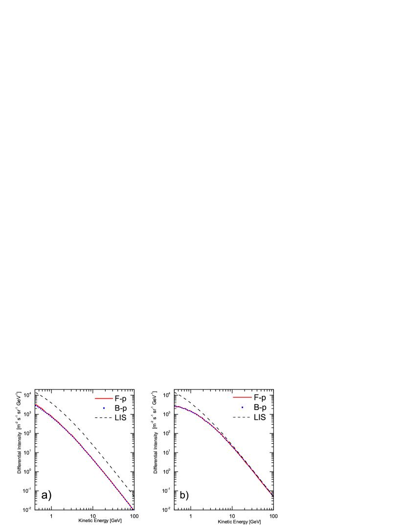
Figure 1: Monte Carlo solutions obtained with the F-p (red line) and B-p (blue dot). In figure a) the diffusion coefficient is taken to be independent from rigidity (see eq. (3.1)), i.e., the diffusion process is the same at any energies as well as the flux reduction. In figure b) the diffusion coefficient is scaled according to eq. (3.2), i.e., at higher rigidities the diffusion process is less efficient and, then, GCR spectrum is less modulated.

4 Conclusion

HelMod Model allows user to evaluate the modulated spectrum of GCR inside heliosphere solving the Parker’s equation using a Monte Carlo Technique involving SDE. We developed two different algorithms solving the SDEs forward-in-time and backward-in-time. We show that the two solutions are equivalent and suitable to provide solutions of the modulated spectrum with a relative systematic uncertainty below of $5\%$, that is the typical error bar of GeV experimental data.

- [1] E. N. Parker, The passage of energetic charged particles through interplanetary space, Plan. Space Sci. 13 (1965) 9.
- [2] L. J. Gleeson and W. I. Axford, Solar Modulation of Galactic Cosmic Rays, Astrophys. J. 154 (Dec., 1968) 1011.
- [3] L. J. Gleeson and I. H. Urch, Energy losses and modulation of galactic cosmic rays., Astrophys. Space Sci. 11 (May, 1971) 288–308.
- [4] L. J. Gleeson and I. H. Urch, A Study of the Force-Field Equation for the Propagation of Galactic Cosmic Rays, Astrophys. Space Sci. 25 (Dec., 1973) 387–404.
- [5] R. A. Caballero-Lopez and H. Moraal, Limitations of the force field equation to describe cosmic ray modulation, J. Geophys. Res.-Space 109 (Jan., 2004) 1101.
- [6] J. R. Jokipii and D. A. Kopriva, Effects of particle drift on the transport of cosmic rays. III - Numerical models of galactic cosmic-ray modulation, Astrophys. J. 234 (Nov., 1979) 384–392.
- [7] M. S. Potgieter and H. Moraal, A drift model for the modulation of galactic cosmic rays, Astrophys. J. 294 (1985), no. part 1 425–440.
- [8] P. Bobik, G. Boella, M. J. Boschini, C. Consolandi, S. Della Torre, M. Gervasi, D. Grandi, K. Kudela, S. Pensotti, P. G. Rancoita, and M. Tacconi, Systematic Investigation of Solar Modulation of Galactic Protons for Solar Cycle 23 Using a Monte Carlo Approach with Particle Drift Effects and Latitudinal Dependence, Astrophys. J. 745 (Feb., 2012) 132, [arXiv:1110.4315].
- [9] P. Bobik, G. Boella, M. J. Boschini, C. Consolandi, S. Della Torre, M. Gervasi, D. Grandi, K. Kudela, S. Pensotti, P. G. Rancoita, D. Rozza, and M. Tacconi, Latitudinal Dependence of Cosmic Rays Modulation at 1 AU and Interplanetary Magnetic Field Polar Correction, Advances in Astronomy 2013 (2013) [arXiv:1212.1559].
- [10] P. E. Klöden and E. Platen, Numerical Solution of Stochastic Differential Equations. Springer Edition, 1999.
- [11] J. R. Jokipii and A. J. Owens, Implications of observed charge states of low-energy solar cosmic rays, J. Geophys. Res. 80 (Apr., 1975) 1209–1212.
- [12] J. R. Jokipii and E. H. Levy, Effects of particle drifts on the solar modulation of galactic cosmic rays, Astrophys. J. Lett. 213 (Apr., 1977) L85–L88.
- [13] Y. Yamada, S. Yanagita, and T. Yoshida, A stochastic view of the solar modulation phenomena of cosmic rays, Geophys. Res. Lett. 25 (July, 1998) 2353–2356.
- [14] M. Zhang, A Markov Stochastic Process Theory of Cosmic-Ray Modulation, Astrophys. J. 513 (Mar., 1999) 409–420.
- [15] K. Alanko-Huotari, I. G. Usoskin, K. Mursula, and G. A. Kovaltsov, Stochastic simulation of cosmic ray modulation including a wavy heliospheric current sheet, J. Geophys. Res. 112 (2007), no. A8.
- [16] C. Pei, J. W. Bieber, R. A. Burger, and J. Clem, A general time-dependent stochastic method for solving Parker’s transport equation in spherical coordinates, J. Geophys. Res.-Space 115 (Dec., 2010) 12107.
- [17] R. D. Strauss, M. S. Potgieter, I. Büsching, and A. Kopp, Modeling the Modulation of Galactic and Jovian Electrons by Stochastic Processes, Astrophys. J. 735 (July, 2011) 83.
- [18] S. Della Torre, P. Bobik, M. J. Boschini, C. Consolandi, M. Gervasi, D. Grandi, K. Kudela, S. Pensotti, P. G. Rancoita, D. Rozza, and M. Tacconi, Effects of solar modulation on the cosmic ray positron fraction, Adv. Space Res. 49 (June, 2012) 1587–1592.
- [19] P. Bobik, G. Boella, M. J. Boschini, S. Della Torre, M. Gervasi, D. Grandi, G. La Vacca, K. Kudela, S. Pensotti, P. G. Rancoita, D. Rozza, and M. Tacconi, Cosmic Ray Modulation studied with HelMod Monte Carlo tool and comparison with Ulysses Fast Scan Data during consecutive Solar Minimums , in Proceeding of the 33rd ICRC, 2–9 July, Rio de Janeiro, International Cosmic Ray Conference, p. 1100, 2013. arXiv:1307.5199.
- [20] J. R. Jokipii and E. N. Parker, on the Convection, Diffusion, and Adiabatic Deceleration of Cosmic Rays in the Solar Wind, Astroph. J. 160 (May, 1970) 735.
- [21] L. Fisk, Solar modulation of galactic cosmic rays, J. Geophys. Res.-Space 76 (1971), no. 1 221.
- [22] A. Kopp, I. Büsching, R. D. Strauss, and M. S. Potgieter, A stochastic differential equation code for multidimensional Fokker-Planck type problems, Comput. Phys. Commun. 183 (Mar., 2012) 530–542.
- [23] R. Trotta, G. Jóhannesson, I. V. Moskalenko, T. A. Porter, R. Ruiz de Austri, and A. W. Strong, Constraints on Cosmic-ray Propagation Models from A Global Bayesian Analysis, Astroph. J. 729 (Mar., 2011) 106, [arXiv:1011.0037].
- [24] D. P. Kroese, T. Taimre, and Z. I. Botev, Handbook of Monte Carlo methods. Wiley, 2011.
- [25] C. Gardiner, Handbook of stochastic methods: for physics, chemistry and natural sciences. Springer Edition, 1985.
- [26] D. J. Higham, An Algorithmic Introduction to Numerical Simulation of Stochastic Differential Equations, SIAM Review 43 (Jan., 2001) 525–546.
- [27] M. Gervasi, P. G. Rancoita, I. G. Usoskin, and G. A. Kovaltsov, Monte-Carlo approach to Galactic Cosmic Ray propagation in the Heliosphere, Nucl. Phys. B - Proc. Sup. 78 (Aug., 1999) 26–31.