Abstract

We extend previously proposed measures of complexity, emergence, and self-organization to continuous distributions using differential entropy. This allows us to calculate the complexity of phenomena for which distributions are known. We find that a broad range of common parameters found in Gaussian and scale-free distributions present high complexity values. We also explore the relationship between our measure of complexity and information adaptation.

10.3390/—— xx Received: xx / Accepted: xx / Published: xx Measuring the Complexity of Continuous Distributions Guillermo Santamaría-Bonfil ^1,2*, Nelson Fernández ^3,4* and Carlos Gershenson ^1,2,5,6,7* [2]guillermo.santamaria@iimas.unam.mx, nfernandez@unipamplona.edu.co,cgg@unam.mx.

1 Introduction

We all agree that complexity is everywhere. Yet, there is no agreed definition of complexity. Perhaps complexity is so general that it resists definition Gershenson (2008). Still, it is useful to have formal measures of complexity to study and compare different phenomena Prokopenko et al. (2009). We have proposed measures of emergence, self-organization, and complexity Gershenson and Fernández (2012); Fernández et al. (2014) based on information theory Shannon (1948). Shannon information can be seen as a measure of novelty, so we use it as a measure of emergence, which is correlated with chaotic dynamics. Self-organization can be seen as a measure of order Gershenson and Heylighen (2003), which can be estimated with the inverse of Shannon’s information and is correlated with regularity. Complexity can be seen as a balance between order and chaos Langton (1990); Kauffman (1993), between emergence and self-organization Lopez-Ruiz et al. (1995); Fernández et al. (2014).

We have studied the complexity of different phenomena for different purposes Zubillaga et al. (2014); Amoretti and Gershenson (2015); Febres et al. (2015); Santamaría-Bonfil et al. (2016); Fernández et al. (Submitted). Instead of searching for more data and measure its complexity, we decided to explore different distributions with our measures. This would allow us to study broad classes of dynamical systems in a general way, obtaining a deeper understanding of the nature of complexity, emergence, and self-organization. Nevertheless, our previously proposed measures use discrete Shannon information. Even when any distribution can be discretized, this always comes with caveats  Cover and Thomas (2005). For this reason, we base ourselves on differential entropy  Cover and Thomas (2005); Michalowicz et al. (2013) to propose measures for continuous distributions.

The next section provides background concepts related to information and entropies. Next, discrete measures of emergence, self-organization, and complexity are reviewed Fernández et al. (2014). Section 4 presents continuous versions of these measures, based on differential entropy. The probability density functions used in the experiments are described in Section 5. Section 6 presents results, which are discussed and related to information adaptation Haken and Portugali (2015) in Section 7.

2 Information Theory

Let us have a set of possible events whose probabilities of occurrence are $p_{1},p_{2},\ldots,p_{n}\in P\left(X\right)$. Can we measure the uncertainty described by the probability distribution $P\left(X\right)$? To solve this endeavor in the context of telecommunications, Shannon proposed a measure of entropy Shannon (1948), which corresponds to Boltzmann-Gibbs entropy in thermodynamics. This measure as originally proposed by Shannon, possess a dual meaning of both uncertainty and information, even when the latter term was later discouraged by Shannon himself Heylighen and Joslyn (2003). Moreover, we encourage the concept of entropy as the average uncertainty given the property of asymptotic equipartition (described later in this section). From an information-theoretic perspective, entropy measures the average number of binary questions required to determine the value of $p_{i}$ . In cybernetics, it is related to variety Ashby (1956), a measure of the number of distinct states a system can be in.

In general, entropy is discussed regarding a discrete probability distribution. Shannon extended this concept to the continuous domain with differential entropy. However, some of the properties of its discrete counterpart are not maintained. This has relevant implications for extending to the continuous domain the measures proposed in Gershenson and Fernández (2012); Fernández et al. (2014). Before delving into these differences, first we introduce the discrete entropy, the asymptotic equipartition property (AEP), and the properties of discrete entropy. Next, differential entropy is described, along with its relation to discrete entropy.

2.1 Discrete Entropy

Let $X$ be a discrete random variable, with a probability mass function $p\left(x\right)=Pr\left\{X=x\right\},x\in X$ . The entropy $H\left(X\right)$ of a discrete random variable X is then defined by

$$H\left(X\right)=-\sum_{x\in X}p\left(x\right)\log_{2}p\left(x\right).$$ (1)

The logarithm base provides the entropy’s unit. For instance, base two measures entropy as bits, base ten as nats. If the base of the logarithm is $\beta$, we denote the entropy as $H_{\beta}\left(X\right)$. Unless otherwise stated, we will consider all logarithms to be of base two. Note that entropy does not depend on the value of $X$, but on the probabilities of the possible values $X$ can take. Furthermore, Eq. 1 can be understood as the expected value of the information of the distribution.

2.2 Asymptotic Equipartition Property for Discrete Random Variables

In probability, the large numbers law states that, for a sequence of n i.i.d. elements of a sample $X$, the average value of the sample $\frac{1}{n}\sum_{i=1}^{n}X_{i}$ approximates the expected value $\mathbb{E}\left(X\right)$. In this sense, the Asymptotic Equipartition Property (AEP) establishes that $H\left(X\right)$ can be approximated by

$$H\left(X\right)\mbox{=}\frac{1}{n}\log_{2}\frac{1}{p\left(X_{1},\ldots,X_{n}\right)},$$

such that $n\rightarrow\infty$, and $x_{i}\in X$ are i.i.d. (independent and identically distributed).

Therefore, discrete entropy can be written also as

$$H\left(X\right)=\mathbb{E}\left[\log\frac{1}{p\left(X\right)}\right],$$ (2)

where $\mathbb{E}$ is the expected value of $P\left(X\right).$ Consequently, Eq. 2 describes the expected or average uncertainty of probability distribution $P\left(X\right).$

A final note about entropy is that, in general, any process that makes the probability distribution more uniform increases its entropy Cover and Thomas (2005).

2.3 Properties of Discrete Entropy

The following are properties of the discrete entropy function. Proofs and details can be found in texbooks  Cover and Thomas (2005).

1. Entropy is always non-negative, $H\left(X\right)\geq 0.$

2. $H_{\beta}\left(X\right)=\left(\log_{\beta}a\right)H_{a}\left(X\right).$

3. $H\left(X_{1},X_{2},\ldots,X_{n}\right)\leq\sum_{i=1}^{n}H\left(X_{i}\right),$ with equality iff $X_{i}$ are i.i.d.

4. $H\left(X\right)\leq\log\left|X\right|,$ with equality iff $X$ is distributed uniformly over $X$.

5. $H\left(X\right)$ is concave.

2.4 Differential Entropy

Entropy was first formulated for discrete random variables, and was then generalized to continuous random variables in which case it is called differential entropy Michalowicz et al. (2008). It has been related to the shortest description length, and thus, is similar to the entropy of a discrete random variable Calmet and Calmet (2005). The differential entropy $H\left(X\right)$ of a continuous random variable $X$ with a density $f\left(x\right)$ is defined as

$$H\left(f\right)=H\left(X\right)=-\intop_{S}f\left(x\right)\log_{2}f\left(x\right)dx,$$ (3)

where $S$ is the support set of the random variable. It is well-known that this integral exists iff the density function of the random variables is Riemann-integrable Cover and Thomas (2005); Michalowicz et al. (2013). The Riemann integral is fundamental in modern calculus. Loosely speaking, is the approximation of the area under any continuous curve given by the summation of ever smaller sub-intervals (i.e. approximations), and implies a well-defined concept of limit  Calmet and Calmet (2005). $H\left(f\right)$ can also be used to denote differential entropy, and in the rest of the article, we shall employ this notation.

2.5 Asymptotic Equipartition Property of Continuous Random Variables

Given a set of i.i.d. random variables drawn from a continuous distribution with probability density $f\left(x\right)$, its differential entropy $H\left(f\right)$ is given by

$$-\frac{1}{n}\log_{2}\left(f\left(X_{1},\ldots,X_{n}\right)\right)\rightarrow\mathbb{E}\left[\log_{2}\left(f\left(X\right)\right)\right]=H\left(f\right),$$ (4)

such that $n\rightarrow\infty$. The convergence to expectation is a direct application of the weak law of large numbers.

2.6 Properties of Differential Entropy

1. $H\left(f\right)$ depends on the coordinates.

   For different choices of coordinate systems for a given probability distribution $P\left(X\right)$, the corresponding differential entropies might be distinct.

2. $H\left(f\right)$ is scale variant Cover and Thomas (2005); Yeung (2008).

   In this sense, $H\left(af\right)=H\left(f\right)+\log_{2}\left|a\right|$, such that $a\neq 0$.

3. $H\left(f\right)$is traslational invariant Cover and Thomas (2005); Yeung (2008); Michalowicz et al. (2013).

   In this sense, $H\left(f+c\right)=H\left(f\right)$.

4. $-\infty\leq H\left(f\right)\leq\infty$.  Michalowicz et al. (2013).

   The $H\left(f\right)$ of a Dirac delta probability distribution, is considered the lowest $H\left(f\right)$bound, which corresponds to $H\left(f\right)=-\infty$.

5. Information measures such as relative entropy and mutual information are consistent, either in the discrete or continuous domain Yeung (2008).

2.7 Differences between Discrete and Continuous Entropies

The derivation of equation 3 comes from the assumption that its probability distribution is Riemann-integrable. If this is the case, then differential entropy can be defined just like discrete entropy. However, the notion of “average uncertainty” carried by the Eq. 1 cannot be extended to its differential equivalent. Differential entropy is rather a function of the parameters of a distribution function, that describes how uncertainty changes as the parameters are modified Cover and Thomas (2005).

To understand the differences between Eqs. 1 and 3 we will quantize a probability density function, and then calculate its discrete entropy Cover and Thomas (2005); Michalowicz et al. (2013).

First, consider the continuous random variable $X$ with a probability density function $f\left(x\right).$This function is then quantized by dividing its range into h bins of length $\Delta$. Then, in accordance to the Mean Value Theorem, within each $h_{i}$ bin of size $\left[i\Delta,\left(i+1\right)\Delta\right]$, there exists a value $x_{i}^{*}$ that satisfies

$$\intop_{i\Delta}^{\left(i+1\right)\Delta}f\left(x\right)dx=f\left(x_{i}^{*}\right)\Delta.$$ (5)

Then, a quantized random variable $X_{i}^{\Delta}$is defined as

$$X_{i}^{\Delta}=x_{i}^{*} \text{if }i\Delta\leq X\leq\left(i+1\right)\Delta,$$ (6)

and, its probability is

$$p_{i}=\int_{i\Delta}^{\left(i+1\right)\Delta}X^{\Delta}=f\left(x_{i}^{*}\right)\Delta.$$ (7)

Consequently, the discrete entropy of the quantized variable $X^{\Delta}$, is formulated as

$$H\left(X^{\Delta}\right) = -\sum_{-\infty}^{\infty}p_{i}\log_{2}p_{i}$$ (8)

$$= -\sum_{-\infty}^{\infty}\left(f\left(x_{i}^{*}\right)\Delta\right)\log_{2}\left(f\left(x_{i}^{*}\right)\Delta\right)$$

$$= -\sum\Delta f\left(x_{i}^{*}\right)\log_{2}f\left(x_{i}^{*}\right)-\sum f\left(x_{i}^{*}\right)\Delta\log_{2}\Delta$$

$$= -\log_{2}\Delta-\sum\Delta f\left(x_{i}^{*}\right)\log_{2}f\left(x_{i}^{*}\right).$$

To understand the final form of Eq. 8, notice that as the size of each bin becomes infinitesimal, $\Delta\rightarrow 0$, the left-hand term of Eq. 8 becomes $\log_{2}\left(\Delta\right)$. This is a consequence of

$$\lim_{\Delta\rightarrow 0}\sum_{-\infty}^{\infty}f\left(x_{i}^{*}\right)\Delta=\int_{-\infty}^{\infty}f\left(x\right)dx=1.$$

Furthermore, as $\Delta\rightarrow 0$, the right-hand side of Eq. 8 approximates the differential entropy of X such that

$$\lim_{\Delta\rightarrow 0}\sum_{-\infty}^{\infty}\Delta f\left(x_{i}^{*}\right)\log_{2}f\left(x_{i}^{*}\right)=\int_{-\infty}^{\infty}f\left(x\right)\log_{2}f\left(x\right)dx.$$

Note that the left-hand side of Eq. 8, explodes towards minus infinity such that

$$\lim_{\Delta\rightarrow 0}\log_{2}\left(\Delta\right)\approx-\infty,$$

Therefore, the difference between $H\left(f\right)$ and $H\left(X^{\Delta}\right)$is $H\left(f\right)-H\left(X^{\Delta}\right)=\log_{2}\left(\Delta\right)$, which approaches to $-\infty$ as the bin size becomes infinitesimal. Moreover, consistently with this is the fact that the differential entropy of a discrete value is $-\infty$ Michalowicz et al. (2013).

Lastly, in accordance to Cover and Thomas (2005), the average number of bits required to describe a continuous variable X with a n-bit accuracy (quantization) is $H\left(X\right)+n\approx H\left(f\right)$ such that

$$H\left(X^{\Delta}\right)^{\prime}=\lim_{\Delta\rightarrow 0}H\left(X^{\Delta}\right)+\log_{2}\left(\Delta\right)\rightarrow H\left(f\right).$$ (9)

3 Discrete Complexity Measures

Emergence $E$, self-organization $S$, and complexity $C$ are close relatives of Shannon’s entropy. These information-based measures, inherit most of the properties of Shannon’s discrete entropy Fernández et al. (2014), being the most valuable one that, discrete entropy quantizes the average uncertainty of a probability distribution. In this sense, complexity $C$ and its related measures ($E$ and $S$) are based on a quantization of the average information contained by a process described by its probability distribution.

3.1 Emergence

Another form of entropy, rather related to the concept of information as uncertainty, is called emergence $E$ Fernández et al. (2014). Intuitively, $E$ measures the ratio of uncertainty a process produces by new information that is consequence of changes in a) dynamics or b) scale Fernández et al. (2014). However, its formulation is more related to the thermodynamics entropy. Thus, it is defined as

$$E\equiv H\left(X\right)=-K\sum_{i=1}^{N}p_{i}\log_{2}p_{i},$$ (10)

where $p_{i}=P\left(X=x\right)$ is the probability of the element $i$, and $K$ is a normalizing constant.

3.2 Multiple Scales

In thermodynamics, the Boltzmann constant K, is employed to normalize the entropy in accordance to the probability of each state. However, Shannon’s entropy typical formulation Cover and Thomas (2005); Michalowicz et al. (2013); Haken and Portugali (2015) neglects the usage of K in Eq. 10 (been its only constraint that $K>0,$ Fernández et al. (2014)). Nonetheless, for emergence as a measure of the average production of information for a given distribution, K plays a fundamental role. In the cybernetic definition of variety Heylighen and Joslyn (2003), $K$ is a function of the distinct states a system can be, i.e. the system’s alphabet size. Formally, it is defined as

$$K=\frac{1}{\log_{2}\left(b\right)},$$ (11)

where $b$ corresponds to the size of the alphabet of the sample or bins of a discrete probability distribution. Furthermore, $K$ should guarantee that $0\leq E\leq 1$, therefore, $b$ should be at least equal to the number of bins of the discrete probability distribution.

It is also worth noting that the denominator of Eq. 11, $\log_{2}\left(b\right),$ is equivalent to the maximum entropy for a continuous distribution function, the uniform distribution. Consequently, emergence can be understood as the ratio between the entropy for given distribution $P\left(X\right)$, and the maximum entropy for the same alphabet size $H\left(U\right)$ Singh (2013), this is

$$E=\frac{H\left(P\left(X\right)\right)}{H\left(U\right)}.$$ (12)

3.3 Self-Organization

Entropy can also provide a measure of system’s organization, and its predictability Singh (2013). In this sense, with more uncertainty less predictability is achieved, and vice-versa. Thus, an entirely random process (e.g. uniform distribution) has the lowest organization, and a completely deterministic system one (Dirac delta distribution), has the highest. Furthermore, an extremely organized system yields no information with respect of novelty, while, on the other hand, the more chaotic a system is, the more information is yielded Singh (2013); Fernández et al. (2014).

The metric of self-organization $S$ was proposed to measure the organization a system has regarding its average uncertainty Gershenson (2012); Fernández et al. (2014). $S$ is also related to the cybernetic concept of constraint, which measures changes in due entropy restrictions on the state space of a system Kauffman (1993). These constraints confine the system’s behavior, increasing its predictability, and reducing the (novel) information it provides to an observer. Consequently, the more self-organized a system is, the less average uncertainty it has. Formally, $S$ is defined as

$$S=1-E=1-\left(\frac{H\left(P\left(X\right)\right)}{H\left(U\right)}\right),$$ (13)

such that $0\leq S\leq 1$. It is worth noting that, $S$ is the complement of $E$. Moreover, the maximal $S$ (i.e. $S=1$) is only achievable when the entropy for a given probability density function (PDF) is such that $H\left(P\left(X\right)\right)\rightarrow 0$, which corresponds to the entropy of a Dirac delta (only in the discrete case).

3.4 Complexity

Complexity $C$ can be described as a balance between order (stability), and chaos (scale or dynamical changes) Fernández et al. (2014). More precisely, this function describes a system’s behavior in terms of the average uncertainty produced by its probability distribution in relation the dynamics of a system. Thus, the complexity measure is defined as

$$C=4\cdot E\cdot S,$$ (14)

such that, $0\leq C\leq 1$.

4 Continuous Complexity Measures

As mentioned before, discrete and differential entropies do not share the same properties. In fact, the property of discrete entropy as the average uncertainty in terms of probability, cannot be extended to its continuous counterpart. As consequence, the proposed continuous information-based measures describe how the production of information changes respect to the probability distribution parameters. In particular, this characteristic could be employed as a feature selection method, where the most relevant variables are those which have a high emergence (the most informative).

The proposed measures are differential emergence ($E_{D}$), differential self-organization ($S_{D}$), and differential complexity ($C_{D}$). However, given that the interpretation and formulation (in terms of emergence) of discrete and continuous $S$ (Eq. 13) and $C$ (Eq. 14) are the same, we only provide details on $E_{D}$. The difference between $S_{D}$, $C_{D}$ and $S,C$ is that the former are defined on $E_{D}$, while the latter on $E$. Furthermore, we make emphasis in the definition of the normalizing constant K, which play a significant role in constraining $E_{D}\in\left[0,1\right]$, and consequently, $S_{D}$ and $C_{D}$ as well.

4.1 Differential Emergence

As for its discrete form, the emergence for continuous random variables is defined as

$$E_{D}=-K\intop_{\upsilon}^{\zeta}f\left(X\right)\log_{2}f\left(X\right),$$ (15)

where, $\left[\upsilon,\zeta\right]$ is the domain, and K stands for a normalizing constant related to the distribution’s alphabet size. It is worth noting that this formulation is highly related to the view of emergence as the ratio of information production of a probability distribution respect the maximum differential entropy for the same range. However, since $E_{D}$ can be negative (i.e. entropy of a single discrete value), we choose $E_{D}$ such that

$$E^{\prime}_{D}=\begin{cases}E{}_{D}&E{}_{D}>0\\ 0&\text{otherwise}.\end{cases}.$$ (16)

$E^{\prime}{}_{D}$ is rather a more convenient function than $E{}_{D}$, as $0\leq E^{\prime}{}_{D}\leq 1$. This statement is justified in the fact that the differential entropy of a discrete value is $-\infty$ Cover and Thomas (2005). In practice, differential entropy becomes negative only when the probability distribution is extremely narrow, i.e. there is a high probability for few states. In the context of information changes due parameters manipulation, an $E{}_{D}<0$ means that the probability distribution is becoming a Dirac delta distribution. For notation convenience, from now on we will employ $E_{D}$ and $E^{\prime}_{D}$ interchangeably.

4.2 Multiple Scales

The $K$ constant expresses the relation between uncertainty of a given $P\left(X\right)$ Defined by $H(X)$, respect to the entropy of a maximum entropy over the same domain Singh (2013). In this setup, as the uncertainty grows, $E^{\prime}_{D}$ becomes closer to unity.

To constrain the value of $H\left(X\right)=\left[0,1\right]$ in the discrete emergence case, it was enough to establish the distribution’s alphabet size, b of Eq. 10, such that $b\geq\text{\# bins}$ Fernández et al. (2014). However, for any PDF, the number of elements between a pair of points $a$ and $b$, such that $a\neq b$, is infinite. Moreover, as the size of each bin becomes infinitesimal, $\Delta\rightarrow 0$, the entropy for each bin becomes $-\infty$ Cover and Thomas (2005). Also, it has been stated that b value should be equal to the cardinality of $X$ Singh (2013), however, this applies only to discrete emergence. Therefore, rather than a generalization, we propose an heuristic for the selection of a proper K in the case of differential emergence. Moreover, we differentiate between b for $H\left(f\right)$, and b’ for $H\left(X^{\Delta}\right)^{\prime}$.

As in the discrete case, K is defined as Eq. 11. In order to determine the proper alphabet size b, we propose the next algorithm:

1. If we know a priori the true $P\left(X\right)$, we calculate $H\left(f\right)$, and $b=\left|P\left(X\right)\right|$ is the cardinality within the interval of Eq. 15. In this sense, a large value will denote the cardinality of an “ghost” sample Michalowicz et al. (2013).

2. If we do not know the true $P\left(X\right)$, or we are interested rather in $H\left(X^{\Delta}\right)^{\prime}$ where a sample of finite size is involved, we calculate b’ as

   $$b^{\prime}=\sum_{i}ind\left(x_{i}\right)$$ , (17)

   such that, the non-negative function $ind\left(\cdot\right)$ is defined as

   $$ind\left(x_{i}\right)=\begin{cases}1&\text{iff }P\left(x_{i}\right)>0\\ 0&\text{otherwise}\end{cases}.$$ (18)

   For instance, in the quantized version of the standard normal distribution ($N\left(0,1\right)$), only values within $\pm 3\sigma$ satisfy this constraint despite the domain of Eq. 15. In particular, if we employ $b=\left|X\right|$ rather than $b^{\prime}$, we compress the $E_{D}$ value as it will be shown in the next section. On the other hand, for a uniform distribution or a power-law (such that $0<x_{min}<x$), the whole range of points satisfies this constraint.

5 Probability Density Functions

In communication and information theory, uniform (U) and normal, a.k.a. Gaussian (G) distributions play a significant role. Both are referent to maximum entropy: on the one hand, U has the maximum entropy within a continuous domain; on the other hand, G has the maximum entropy for distributions with a fixed mean ($\mu$), and a finite support set for a fixed standard deviation ($\sigma$) Cover and Thomas (2005); Michalowicz et al. (2013). Moreover, as mentioned earlier, $H\left(f\right)$ is useful when comparing the entropies of two distributions over some reference space Cover and Thomas (2005); Sharma and Sharma (2006); Michalowicz et al. (2013). Consequently, U, but mainly G, are heavily used in the context of telecommunications for signal processing Michalowicz et al. (2013). Nevertheless, many natural and man-made phenomena can be approximated with power-law (PL) distributions. These types of distributions typically present complex patterns that are difficult to predict, making them a relevant research topic Dover (2004). Furthermore, power-laws have been related to the presence of multifractal structures in certain types of processes Sharma and Sharma (2006). Moreover, power-laws are tightly related to self-organization and criticality theory, and have been studied under information frameworks before (e.g. Tsallis’, and Renyi’s maximum entropy principle) Bashkirov and Vityazev (2000); Dover (2004).

Therefore, in this work we focus our attention to these three PDFs. First, we provide a short description of each PDF, then, we summarize its formulation, and the corresponding $H\left(f\right)$ in Table 1.

5.1 Uniform Distribution.

The simplest PDF, as its name states, establishes that for each possible value of X, the probability is constant over the whole support set (defined by the range between $a$ and $b$), and 0 elsewhere. This PDF has no parameters besides the starting and ending points of the support set. Furthermore, this distribution appears frequently in signal processing as white noise, and it has the maximum entropy for continuous random variables Michalowicz et al. (2013).

Its PDF, and its corresponding $H\left(f\right)$ are shown in first row of Table 1. It is worth noting that, as the cardinality of the domain of U grows, its differential entropy increases as well.

5.2 Normal Distribution.

The normal or Gaussian distribution is one of the most important probability distribution families Ahsanullah et al. (2014). It is fundamental in the central limit theorem Michalowicz et al. (2013), time series forecasting models such as classical autoregressive models Box et al. (2008), modelling economic instruments Mitzenmacher (2009), encryption, modelling electronic noise Michalowicz et al. (2013), error analysis and statistical hypothesis testing.

Its PDF is characterized by a symmetric, bell-shaped function whose parameters are: location (i.e. mean $\mu$), and dispersion (i.e. standard deviation $\sigma^{2}$ ). The standard normal distribution is the simplest and most used case of this family, its parameters are $N\left(\mu=0,\,\sigma^{2}=1\right)$. A continuous random variable $x\in X$ is said to belong to a Gaussian distribution, $X\sim N\left(\mu,\,\sigma^{2}\right)$ , if its PDF $p\left(x\right)$ is given by the one described in the second row of Table 1. As is shown in the table, the differential entropy of G only depends on the standard deviation. Furthermore, it is well known that its differential entropy is monotonically increasing concave in relation to $\sigma$ Ahsanullah et al. (2014). This is consistent with the aforementioned fact that $H\left(f\right)$ is translation-invariant. Thus, as $\sigma$ grows, so does the value of $H\left(G\right)$, while as $\sigma\rightarrow 0$ such that $0<\sigma<1$, it becomes a Dirac delta with $H\left(f\right)\approx 0$.

5.3 Power-Law Distribution.

Power-law distributions are commonly employed to describe multiple phenomena (e.g. turbulence, DNA sequences, city populations, linguistics, cosmic rays, moon craters, biological networks, data storage in organisms, chaotic open systems, and so on) across numerous scientific disciplines Bashkirov and Vityazev (2000); Mitzenmacher (2001); Dover (2004); Sharma and Sharma (2006); Clauset et al. (2009); Frigg and Werndl (2011); Virkar and Clauset (2014). These type of processes are known for being scale invariant, being the typically scales ($\alpha$, see below) in nature between one and 3.5 Bashkirov and Vityazev (2000). Also, the closeness of this type of PDF to chaotic systems and fractals is such that, some fractal dimensions are called entropy dimensions (e.g. box-counting dimension, and Renyi entropy) Frigg and Werndl (2011).

Power-law distributions can be described by continuous and discrete distributions. Furthermore, Power-laws in comparison with Normal distribution, generate events of large orders of magnitude more often, and are not well represented by a simple mean. A Power-Law density distribution is defined as

$$p\left(x\right)dx=P\left(x\leq X\leq x+dx\right)=Cx^{-\alpha}dx,$$ (19)

such that, C is a normalization factor, $\alpha$ is the scale exponent, and $X\mid x>x_{min}>0$ is the observed continuos random variable. This PDF diverges as $x\rightarrow 0$ , and do not hold for all $x\geq 0$ Virkar and Clauset (2014). Thus, $x_{min}$ corresponds to lower bound of a power-law. Consequently, in Table 1 we provide the PDF of a Power-Law as proposed by Clauset et al. (2009), and its corresponding $H\left(f\right)$ as proposed by Yapage (2014).

The aforementioned PDFs, and their corresponding $H\left(f\right)$ are shown in Table 1. Further details about the derivation of $H\left(f\right)$ for U, and G can be found in Cover and Thomas (2005); Michalowicz et al. (2013). For additional details on the differential entropy of the power-law, we refer the reader to Sharma and Sharma (2006); Yapage (2014).

Distribution PDF Differential Entropy Uniform $p\mbox{$\left(x\right)$=}\begin{cases}\frac{1}{b-a}&a\leq x\leq b\\ 0&\text{otherwise}\end{cases}$ $H\left(p\left(x\right)\right)=\log_{2}\left(b\right)$ Normal $p\left(x\right)=\frac{1}{\sigma\sqrt{2\pi}}e^{\frac{-\left(x-\mu\right)^{2}}{2\sigma}}$ $H\left(p\left(x\right)\right)=\frac{1}{2}\log_{2}\left(2\pi e\sigma^{2}\right)$ Power-law $p\left(x\right)=\left(\frac{\alpha-1}{x_{min}}\right)\left(\frac{x}{x_{min}}\right)^{-\alpha}$ $H\left(p\left(x\right)\right)=\log_{2}\left(x_{min}\right)-\log_{2}\left(\alpha-1\right)+\left(\frac{\alpha}{\alpha-1}\right)$

Table 1: Studied PDFs (left column) with their corresponding analytical differential entropies (right column).

6 Results

In this section, comparisons of theoretical vs quantized differential entropy for the PDFs considered are shown. Next, we provide differential complexity results ($E^{\prime}_{D}$, $S_{D}$, and $C_{D}$) for the mentioned PDFs. Furthermore, in the case of power-laws, we also provide and discuss the corresponding complexity measures results for real world phenomena, already described in Newman (2005). Also, it is worth noting that, since for quantized $H\left(f\right)$ of the power-law yielded poor results, the power-law’s analytical $H\left(f\right)$ form was used.

6.1 Theoretical vs Quantized Differential Entropies

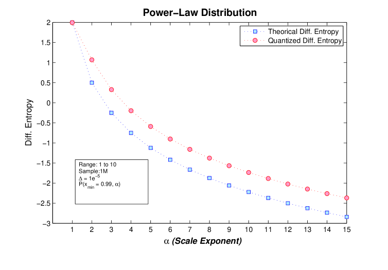
Numerical results of theoretical and quantized differential entropies are shown in Figs. 1 and 2. Analytical $H\left(f\right)$ results are displayed in blue, whereas the quantized $H\left(X^{\Delta}\right)^{\prime}$ ones are shown in red. For each PDF, a sample of one million (i.e. $1\times 10^{6}\equiv\text{1M}$) points where employed for calculations. The bin size $\Delta$ required by $H\left(X^{\Delta}\right)^{\prime}$, is obtained as the ratio $\Delta=\frac{Range}{\left|Sample\right|}$. However, the value of $\Delta$ has considerable influence in the resulting quantized differential entropy.

Figure 1: Theoretical and quantized differential entropies for the uniform and power-law distributions.

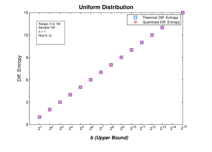
6.1.1 Uniform Distribution.

The results for U were expectable. We tested several values of the cardinality of $P\left(X\right)$, such that $b=2^{i}\mid i=1,\ldots,15$. Using the analytical $H\left(f\right)$ formula of Table 1, the quantized $H\left(X^{\Delta}\right)^{\prime}$, and $\Delta=1$ we achieved exactly the same differential entropy values. Results for U are shown in the left side of Fig. 1. As was mentioned earlier, as the cardinality of the distribution grows, so does the differential entropy of U.

6.1.2 Normal Distribution.

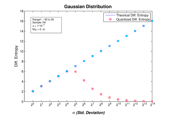
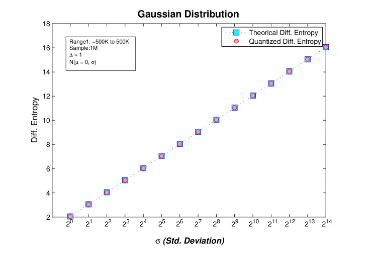
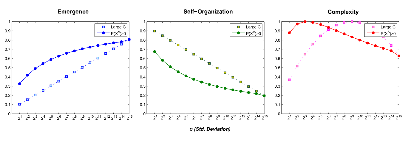
Results for the Gaussian distribution were less trivial. As in the U case, we calculate both $H\left(f\right)$ and $H\left(X^{\Delta}\right)^{\prime}$, for a fixed $\mu=0$, and modified the standard deviation parameter such that, $\sigma=2^{i}\mid i=0,1,\ldots,14$. Notice that the first tested distribution is the standard normal distribution.

In Fig. 2, results obtained for the n-bit quantized differential entropy, and for the analytical form of Table 1 are shown. Moreover, we displayed two cases of the normal distribution: the left side of Fig. 2 shows results for $P\left(X\right)$ with range $\left[-50,50\right]$ and a bin size, $\Delta=\frac{100}{1M}=1\times 10^{-4}$,whereas, right side provides results for a $P\left(X\right)$ with range $\left[-500e3,500e3\right]$ and $\Delta=1$. It is worth noting that, in the former case the quantized differential entropy shows a discrepancy with $H\left(f\right)$ after only $\sigma=2^{4}=16$, which quickly increases with growing $\sigma$. On the other hand, for the latter case there is an almost perfect match between the analytical and quantized differential entropies, however, the same mismatch will be observed if the standard deviation parameter is allowed to grow unboundedly $(\sigma\rightarrow\infty)$. Nonetheless, this is a consequence of how $H\left(X^{\Delta}\right)^{\prime}$ is computed. As mentioned earlier, as $\Delta\rightarrow 0$ the value of each quantized $X^{\Delta}$ grows towards $-\infty$. Therefore, in the G case, it seems convenient employing a Probability Mass Function (PMF) rather than a PDF. Consequently, the experimental setup of right side image of Fig. 2 is employed for the calculation of the continuous complexity measures of G.

Figure 2: Two comparisons of theoretical vs quantized differential entropy for the Gaussian distribution.

6.1.3 Power-Law Distribution.

Results for the power-law distribution are shown in the right side of Fig. 1. In both U and G, a PMF instead of a PDF was used to avoid cumbersome results (as depicted in the corresponding images). However, for the power-law distribution, the use of a PDF is rather convenient. As shown in Fig. 4 and highlighted by Clauset et al. (2009), $x_{min}$ has a considerable impact on the value of $H\left(f\right)$. For Fig. 1, the range employed was $\left[1,50\right]$, with a bin size of $\Delta=1\times 10^{-5}$, a $x_{min}=0.99$, and modified the scale exponent parameter such that, $\alpha=i\mid i=1,\ldots,15$. For this particular setup, we can observe that as $\alpha$ increases, $H\left(f\right)$ and $H\left(X^{\Delta}\right)^{\prime}$ decreases its value towards $-\infty$. This effect is consequence of increasing the scale of the Power-law such that, the slope of the function in a log-log space, approaches to zero. In this sense, with larger $\alpha$’s, the $P\left(X\right)$ becomes closer to a Dirac delta distribution, thus, $H\left(f\right)\rightarrow-\infty$. However, as will be discussed later, for larger $\alpha$’s larger $x_{min}$ values are required, in order for $H\left(f\right)$ to display positive values.

6.2 Differential Complexity: $E{}_{D}$, $S_{D}$, and $C_{D}$

U results are trivial: $E{}_{D}=1$, and $S_{D},C_{D}=0$. For each upper bound of U, $E^{\prime}_{D}=\frac{H\left(U\right)}{H\left(U\right)}=1$, which is exactly the same as its discrete counterpart. Thus, U results are not considered in the following analysis.

Continuous complexity results for G and PL are shown in Figs. 3 and 4, respectively. In the following we provide details of these measures.

6.2.1 Normal Distribution.

It was stated in Section 4 that, the size of the alphabet is given by the function $ind\left(P\left(X\right)\right)$. This rule establishes a valid cardinality such that $P\left(X\right)>0$, thus, only those states with a positive probability are considered. For $P\left(X^{\Delta}\right)$, such operation can be performed. Nevertheless, when the analytical $H\left(f\right)$ is used, the proper cardinality of the set is unavailable. Therefore, in the Gaussian distribution case, we tested two criteria for selecting the value of b:

1. $\sum_{x_{i}}ind\left(\cdot\right)$ is employed for $H\left(X^{\Delta}\right)^{\prime}$

2. A constant with a large value ($C=1\times 10^{6}$) is used for the analytical formula of $H\left(f\right)$.

In Fig. 3, solid dots are used when K is equal to the cardinality of $P\left(X\right)>0$, whereas solid squares are used for an arbitrary large constant. Moreover, for the quantized case of $P\left(G\right)$ , Table 2 shows the cardinality for each sigma, $b^{\prime}_{i}$, and its corresponding $K_{i}$. As it can be observed, for a large normalizing constant K, a logarithmic relation is displayed for $E{}_{D}$ and $S_{D}$. Also, the maximum $C_{D}$ is achieved for $\sigma=2^{8}=256$, which is where $E{}_{D}=S_{D}$. However, for $H\left(X^{\Delta}\right)^{\prime}$ the the maximum $C_{D}$ is found around $\sigma=2^{1,2,3}=2,4,8$, such that $C_{D}\leq\epsilon\mid\epsilon\rightarrow 0$. A word of advise must be made here. The required cardinality to normalize the continuous complexity measures such that $0\leq E{}_{D},S_{D},C_{D}\leq 1$, must have a lower bound. This bound should be related to the scale of the $P\left(X\right)$ Landsberg (1994), and the quantization size $\Delta$. In our case, when a large cardinality $\left|U\right|=1\times 10^{6}$, and $\Delta=1$ are used, the normalizing constant flattens $E_{D}$ results respect those obtained by $b^{\prime}$; moreover, the large constant increases $S_{D}$, and takes greater standard deviations for achieving the maximum $C_{D}$. However, these complexity results are rather artificial in the sense that, if we arbitrarly let $\left|U\right|\rightarrow\infty$ then trivially we will obtain $E{}_{D}=0,\,S_{D}=1,\text{ and }C_{D}=0$. Moreover, it has been stated that the cardinality of $P\left(X\right)$ should be employed as a proper size of b Singh (2013). Therefore, when $H\left(X^{\Delta}\right)^{\prime}$ is employed, the cardinality of $P\left(X\right)>0$ must be used. On the contrary, when $H\left(f\right)$ is employed, a coarse search for increasing alphabet sizes could be used so that the maximal $H\left(f\right)$ satisfies $\frac{H\left(f\right)}{H\left(U\right)}\leq 1$.

$\sigma$	$b^{\prime}=\sum ind\left(Pr\left(X\right)>0\right)$	$H\left(U\right)=\log_{2}\left(b^{\prime}\right)$	$K=\frac{1}{H\left(U\right)}$
$2^{0}=1$	78	6.28	0.16
$2^{1}=2$	154	7.26	0.14
$2^{2}=4$	308	8.27	0.12
$2^{3}=8$	616	9.27	0.11
$2^{4}=16$	1232	10.27	0.10
$2^{5}=32$	2464	11.27	0.09
$2^{6}=64$	4924	12.27	0.08
$2^{7}=128$	9844	13.27	0.075
$2^{8}=256$	19680	14.26	0.0701
$2^{9}=512$	39340	15.26	0.0655
$2^{10}=1024$	78644	16.26	0.0615
$2^{11}=2048$	157212	17.26	0.058
$2^{12}=4096$	314278	18.26	0.055
$2^{13}=8192$	628258	19.26	0.0520
$2^{14}=16384$	1000000	19.93	0.050

Table 2: Alphabet size $b^{\prime}$, and its corresponding normalizing K constant for the normal distribution G.

Figure 3: Complexity of the Gaussian distribution.

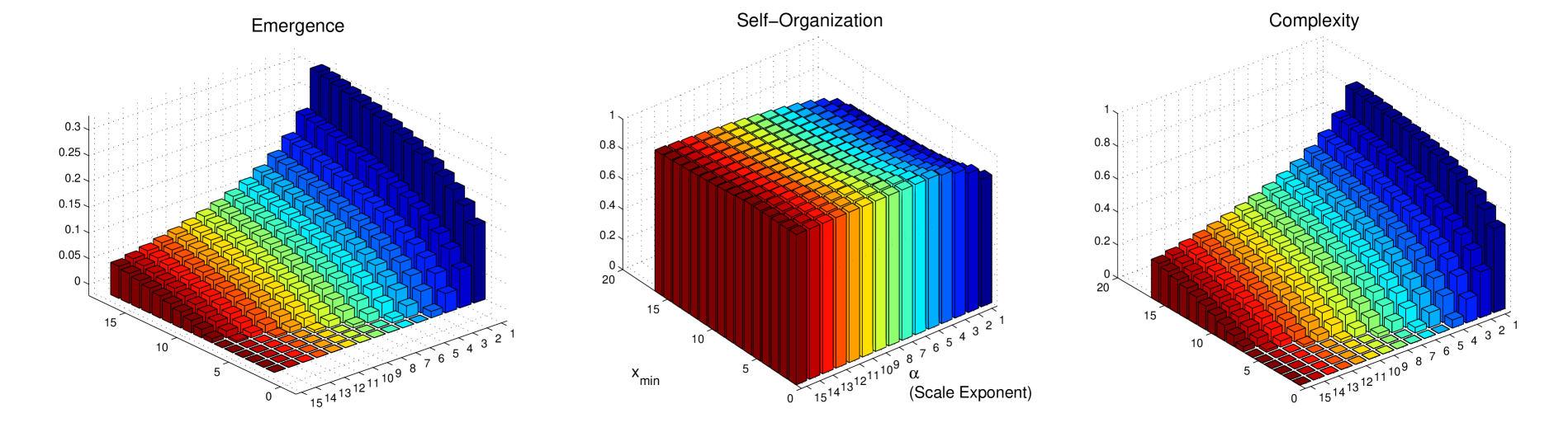
6.2.2 Power-Law Distribution

In this case, $H\left(f\right)$ rather than $H\left(X^{\Delta}\right)^{\prime}$ is used for computational convenience. Although the cardinality of $P\left(X\right)>0$ is not available, by simply substituting $p\left(x_{i}\right)>0\mid x=\left\{1,\ldots,1\times 10^{6}\right\}$ we can see that the condition is fulfilled by the whole set. Therefore, the large $C$ criterium, earlier detailed, is used. Still, given that a numerical power-law distribution is given by two parameters, a lower bound $x_{min}$ and the scale exponent $\alpha$, we depict our results in 3D in Fig. 4. From left to right, $E{}_{D},\,S_{D},\text{ and }C_{D}$ for the power-law distribution are shown, respectively. In the three images, the same coding is used: x-axis displays the scale exponent ($\alpha$) values, y-axis shows $x_{min}$ values, and z-axis depicts the continuous measure values; lower values of $\alpha$ are displayed in dark blue, turning into reddish colors for larger exponents.

As it can be appreciated in Fig. 4, for small $x_{min}$ (e.g. $x_{min}=1$) values, low emergence is produced despite the scale exponent. Moreover, maximal self-organization ($\text{\emph{i.e.} }S_{D}=1$) is quickly achieved (i.e. $\alpha=4$), providing a PL with at most fair complexity values. However, if we let $x_{min}$ take larger numbers, $E_{D}$ grows, achieving the maximal complexity (i.e. $C_{D}\approx 0.8$) of this experimental setup at $x_{min}=15,\,\alpha=1$. This behavior is also observed for other scale exponent values, where emergence of new information is produced as the $x_{min}$ value grows. Furthermore, it has been stated that for $P\left(X\right)$ displays a power-law behavior it is required that $\forall x_{i}\in P\left(X\right)\mid x_{i}>x_{min}$ Virkar and Clauset (2014). Thus, for every $\alpha$ there should be an $x_{min}$ such that $E_{D}>0$. Moreover, for larger scale exponents, larger $x_{min}$ values are required for the distribution shows emergence of new information at all.

6.3 Real World Phenomena and their Complexity

Data of phenomena that follows a power law is provided in Table 3. These power-laws have been studied by Newman (2005); Clauset et al. (2009); Virkar and Clauset (2014), and the power-law parameters were published by Newman (2005). The phenomena in the table mentioned above compromises data from:

1. Numbers of occurrences of words in the novel Moby Dick by Hermann Melville.

2. Numbers of citations to scientific papers published in 1981, from the time of publication until June 1997.

3. Numbers of hits on websites by users of America Online Internet services during a single day.

4. Number of received calls to A.T.&T. U.S. long-distance telephone services on a single day.

5. Earthquake magnitudes occurred in California between 1910 and 1992.

6. Distribution of the diameter of moon craters.

7. Peak gamma-ray intensity of solar flares between 1980 and 1989.

8. War intensity between 1816–1980, where intensity is a formula related to the number of deaths and warring nations populations.

9. Frequency of family names accordance with U.S. 1990 census.

10. Population per city in the U.S. in agreement with U.S. 2000 census.

More details about these power-laws can be found in Newman (2005); Clauset et al. (2009); Virkar and Clauset (2014).

For each phenomenon, the corresponding differential entropy and complexity measures are shown in Table 3. Furthermore, we also provide Table 5 which is a color coding for complexity measures proposed in  Fernández et al. (2014). Five colors are employed to simplify the different value ranges of $E_{D}$, $S_{D}$, and $C_{D}$ results. According to the nomenclature suggested in Fernández et al. (2014), results for these sets show that, very high complexity $0.8\leq C_{D}\leq 1$ is obtained by the number of citations set (i.e. 2), and intensity of solar flares (i.e. 7). High complexity, $0.6\leq C_{D}<0.8$ is obtained for received telephone calls (i.e. 4), intensity of wars (i.e. 8), and frequency of family names (i.e. 9). Fair complexity $0.4\leq C_{D}<0.6$ is displayed by earthquakes magnitude (i.e. 5), and population of U.S. cities (i.e. 10). Low complexity, $0.2\leq C_{D}<0.4$ is obtained for frequency of used words in Moby Dick (i.e. 1) and web hits (i.e. 3), whereas, moon craters (i.e. 6) have very low complexity $0\leq C_{D}<0.2$. In fact, earthquakes, and web hits, have been found not to follow a power law Clauset et al. (2009). Furthermore, if such sets were to follow a power-law, a greater value of $x_{min}$ would be required as can be observed in Fig. 4. In fact, the former case is found for the frequency of words used in Moby Dick. In Newman (2005), parameters of Table 3 are proposed. However, in Clauset et al. (2009), another set of parameters are estimated (i.e. $x_{min}=7,\,\alpha=1.95$). For the more recent estimated set of parameters, a high complexity is achieved (i.e. $C_{D}=0.74$), which is more consistent with literature about Zipf’s law Newman (2005). Lastly, in the case of moon craters, the $x_{min}=0.01$ is rather a poor choice according to Fig. 4. For the chosen scale exponent, it would require at least a $x_{min}\approx 1$, for the power-law to produce any information at all. It should be noted that $x_{min}$ can be adjusted to change the values of all measures. Also, it is worth mentioning that if we were to normalize and discretize a power law distribution to calculate its discrete entropy (as in Fernández et al. (2014)), all power law distributions present a very high complexity, independently of $x_{min}$ and $\alpha$, precisely because these are normalized. Still, this is not useful for comparing different power law distributions.

Figure 4: Complexity measures for the Power-Law. Lower values of the scale exponent $\alpha$ are displayed in dark blue, colors turns into reddish for larger scale exponents.

Phenomenon $x_{min}$ $\alpha$ (Scale Exponent) $H\left(f\right)$ $E^{\prime}_{D}$ $S_{D}$ $C_{D}$ 1 Frequency of use of words 1 2.2 1.57 0.078 0.92 0.29 2 Number of citations to papers 100 3.04 7.1 0.36 0.64 0.91 3 Number of hits on web sites 1 2.4 1.23 0.06 0.94 0.23 4 Telephone calls received 10 2.22 4.85 0.24 0.76 0.74 5 Magnitude of earthquakes 3.8 3.04 2.38 0.12 0.88 0.42 6 Diameter of moon craters 0.01 3.14 -6.27 0 1 0 7 Intensity of solar flares 200 1.83 10.11 0.51 0.49 0.99 8 Intensity of wars 3 1.80 4.15 0.21 0.79 0.66 9 Frequency of family names 10000 1.94 15.44 0.78 0.22 0.7 10 Population of U.S. cities 40000 2.30 16.67 0.83 0.17 0.55

Table 3: Power-Law parameters and information-based measures of real world phenomena

Table 4: Categories for classifying $E$, $S$, and $C$.

Category	Very High	High	Fair	Low	Very Low
Range	$[0.8,1]$	$[0.6,0.8)$	$[0.4,0.6)$	$[0.2,0.4)$	$[0,0.2)$
Color	Blue	Green	Yellow	Orange	Red

Table 5: Color coding for $E_{D}$, $S_{D}$, and $C_{D}$ results

7 Discussion

The relevance of the work presented here lies in the fact that it is now possible to calculate measures of emergence, self-organization, and complexity directly from probability distributions, without needing access to raw data. Certainly, the interpretation of the measures is not given, as this will depend on the use we make of the measures for specific purposes.

From exploring the parameter space of the uniform, normal, and scale-free distributions, we can corroborate that high complexity values require a form of balance between extreme cases. On the one hand, uniform distributions, by definition, are homogeneous and thus all states are equiprobable, yielding the highest emergence. This is also the case of normal distributions with a very large standard deviation and for power law distributions with an exponent close to zero. On the other hand, highly biased distributions (very small standard deviation in G or very large exponent in PL) yield a high self-organization, as few states accumulate most of the probability. Complexity is found between these two extremes. From the values of $\sigma$ and $\alpha$, this coincides with a broad range of phenomena. This does not tell us something new: complexity is common. The relevant aspect is that this provides a common framework to study of the processes that lead phenomena to have a high complexity Gershenson and Lenaerts (2008). It should be noted that this also depends on the time scales at which change occurs Cocho et al. (2015).

In this context, it is interesting to relate our results with information adaptation Haken and Portugali (2015). In a variety of systems, adaptation takes place by inflating or deflating information, so that the “right" balance is achieved. Certainly, this precise balance can change from system to system and from context to context. Still, the capability of information adaptation has to be correlated with complexity, as the measure also reflects a balance between emergence (inflated information) and self-organization (deflated information).

As a future work, it will be interesting to study the relationship between complexity and semantic information. There seems to be a connection with complexity as well, as we have proposed a measure of autopoiesis as the ratio of the complexity of a system over the complexity of its environment Fernández et al. (2014); Gershenson (2015). These efforts should be valuable in the study of the relationship between information and meaning, in particular in cognitive systems.

Another future line of research lies in the relationship between the proposed measures and complex networks Newman (2003); Newman et al. (2006); Boccaletti et al. (2006); Gershenson and Prokopenko (2011), exploring questions such as: how does the topology of a network affect its dynamics? How much can we predict the dynamics of a network based on its topology? What is the relationship between topological complexity and dynamic complexity? How controllable are networks Motter (2015) depending on their complexity?