Boltzmann electron PIC simulation of the E-sail effect

Abstract

The solar wind electric sail (E-sail) is a planned in-space propulsion device that uses the natural solar wind momentum flux for spacecraft propulsion with the help of long, charged, centrifugally stretched tethers. The problem of accurately predicting the E-sail thrust is still somewhat open, however, due to a possible electron population trapped by the tether. Here we develop a new type of particle-in-cell (PIC) simulation for predicting E-sail thrust. In the new simulation, electrons are modelled as a fluid, hence resembling hybrid simulation, but in contrast to normal hybrid simulation, the Poisson equation is used as in normal PIC to calculate the self-consistent electrostatic field. For electron-repulsive parts of the potential, the Boltzmann relation is used. For electron-attractive parts of the potential we employ a power law which contains a parameter that can be used to control the number of trapped electrons. We perform a set of runs varying the parameter and select the one with the smallest number of trapped electrons which still behaves in a physically meaningful way in the sense of producing not more than one solar wind ion deflection shock upstream of the tether. By this prescription we obtain thrust per tether length values that are in line with earlier estimates, although somewhat smaller. We conclude that the Boltzmann PIC simulation is a new tool for simulating the E-sail thrust. This tool enables us to calculate solutions rapidly and allows to easily study different scenarios for trapped electrons.

The electric solar wind sail (electric sail, E-sail) is a planned device for producing interplanetary spacecraft propulsion from the natural solar wind by a set of centrifugally stretched thin metallic tethers that are kept artificially at a high positive potential (Janhunen et al., 2010). In order to engineer E-sail devices in detail, one should predict the magnitude of the Coulomb drag that the flowing solar wind exerts on the charged tether. Thus far this problem has been studied using particle-in-cell (PIC) simulations (Janhunen and Sandroos, 2007; Janhunen, 2009, 2012), Vlasov simulations (Sánchez-Arriaga and Pastor-Moreno, 2014) and other methods (Sanmartín et al., 2008; Sanchez-Torres, 2014). However, a fully satisfactory way of estimating E-sail thrust has not yet emerged, except for negative polarity tethers (Janhunen, 2014a), which are however more suitable to use in low Earth orbit (LEO) as a deorbiting plasma brake device (Janhunen, 2010) than in the solar wind (Janhunen, 2009). Independent laboratory measurements of the width of the electron sheath around a positively biased tether placed in streaming plasma were made by Siguier et al. (2013). The laboratory results were produced in a plasma mimicking conditions in LEO and they are in good agreement with PIC thrust predictions (Janhunen, 2014b).

In this paper we develop a new variant of the PIC simulation of Janhunen (2012) which treats electrons as a fluid obeying the Boltzmann relation, with two additional tricks to be detailed below. The motivation is to have a code which is relatively fast and easy to run and which makes it possible for the user to control the assumed amount of trapped electrons in a simple way. We present the simulation code and use it to derive a thrust estimate in a case which has relevance to the E-sail. Making more comprehensive set of runs with different voltages and in different solar wind conditions is outside of the scope of the paper.

1 Physics of tether Coulomb drag

The negative polarity Coulomb drag effect can be successfully simulated by a PIC code (Janhunen, 2014a). The negative polarity effect is less challenging to simulate than the positive polarity one, because in the negative polarity case, trapped particles do not form. Electrons are not trapped because they are repelled by the tether’s negative potential structure. Ions (protons) are also not trapped, because in relevant cases the surrounding plasma flow is supersonic so that in a coordinate frame where the tether is stationary, ions enter the potential structure with significant kinetic energy and hence cannot be easily trapped by the potential.

In the positive polarity case which is the subject of the present paper, electrons may become trapped because the tether attracts them and because the electron flow is subsonic so that there are some electrons which enter the potential structure with nearly zero initial energy. The issue of trapped electrons was identified by Janhunen and Sandroos (2007) and simulations were later made where chaotisation of trapped electron orbits when scattering at the end of the tether and at the spacecraft was explicitly included in the PIC code, as well as occasional removal of trapped electrons due to collisions with the tether (Janhunen, 2012). However, in that calculation the timescale where trapped electrons were removed was made much faster than in reality, in order to complete the simulation run in a reasonable time. Basically, processes controlling the size of the trapped electron population are poorly known, because we think that they happen at longer timescales than what is accessible by PIC simulation.

Consider a 2-D positive potential structure which thus forms a negative potential energy well (attractive structure) for electrons. If the potential is stationary and hosts no trapped electrons and if the ambient electron distribution is a non-drifting Maxwellian and the plasma is tenuous enough to be collisionless, then it can be shown using Liouville’s theorem that the local electron density can nowhere exceed the background plasma density (Laframboise and Parker, 1973; Janhunen, 2009). In fact, under the stated conditions the electron density is typically significantly less than the background density in most regions covered by the attractive potential structure. Physically the result is due to the fact that although the tether attracts electrons and therefore focusses them to move through its vicinity, the electron density remains low because accelerating the electron reduces the time that the electron spends inside the attractive potential structure. Conservation of the electron’s originally nonzero angular momentum also limits the minimum distance that the electron can have from the tether.

That the electron density nowhere exceeds the background density leads to an interesting dilemma (Éric Choinière, private communication) that is associated with trapped electrons because the ion density, on the other hand, must be higher than the background density inside at least in some regions of the upstream side ion deflection shock. Then, a significant positive charge density can build up at the upstream ion deflection region, which spreads out the electron-attractive potential structure and thus decreases the local electron density further which, unless some process intervenes, makes the charge imbalance worse. What exactly happens remains not well known, but conceivably, instabilities which are able to scatter electrons might develop and take place until enough trapped electrons have been formed so that proper charge neutralisation in the ion deflection shock region has been restored. A simple approach to model this kind of general behaviour may be to reduce the number of trapped electrons in the simulation until the result becomes nonphysical in some way or another and postulate that the most realistic run is the physical run with least amount of trapped electrons. This is what the simulation presented next attempts to accomplish.

2 Simulation code

We use a special version of electrostatic PIC where electrons are not modelled as particles, but as a fluid whose local density $n_{e}(x,y)$ is an assumed function of the local potential $V(x,y)$. When the potential repels electrons (i.e. when $V(x,y)<0$), the Boltzmann relation is assumed,

$$n_{e}(x,y)=n_{\rm o}\exp\left[\frac{eV(x,y)}{T_{e}}\right],\quad\mathrm{when}\ V(x,y)<0$$ (1)

where $n_{\rm o}$ is the background plasma density and $T_{e}=10$ eV is the background electron temperature in energy units. The Boltzmann relation is supposedly a good approximation for the density of particles that try to penetrate thermally into a repulsive potential structure.

For attractive parts of the potential, the electron density depends on the number and distribution function of trapped electrons and thus extra assumptions are needed. That one needs such assumptions is natural because we are not modelling electron dynamics using first principles. We want to have a functional relationship which contains a parameter that can be used to tune the number of trapped electrons in a simple way.

In this paper we use the following functional form for electron density in attractive parts of the potential:

$$n_{e}(x,y)=n_{\rm o}\left[1+\frac{eV(x,y)}{T_{e}}\right]^{\nu}\quad\mathrm{when}\ V(x,y)\geq 0$$ (2)

where $\nu>0$ is the trapped electron control parameter.

In Figure 1 we show how the local electron density depends on the local potential according to Eqs. (1) and (2).

The code that we use in this paper is a descendant of a PIC code that we used earlier (Janhunen and Sandroos, 2007; Janhunen, 2012, 2014a). It is an electrostatic code with linear particle weighting and additional grid-level smoothing which is implemented in the Fourier domain. The code supports 2-D and 3-D simulations and optionally includes a constant external magnetic field. The Poisson solver is implemented by fast Fourier transform and the code is parallelised with OpenMP threads and the Message Passing Interface (MPI) library. The code is also vectorised, so that for a processor with 256-bit wide AVX2 instruction set, each processor core calculates eight particle updates simultaneously. For particle coordinates and velocities, 32-bit floating point accuracy is used. To avoid loss of accuracy, particle coordinates are expressed relative to the centroid of the grid cell where the particle resides. Particles are stored in lists belonging to grid cells which enables fast accumulation of the charge density (no irregular memory addressing patterns needed) and enables good data locality and cache friendliness. When a particle crosses a grid cell boundary, it is removed from the old list and entered into a new one.

An additional trick is needed to avoid solutions that look unphysical and oscillate drastically in time. Namely, the electron density must not react instantaneously to changed electric potential, but with some delay. If $n_{e}^{*}(x,y)$ is the preliminary instantaneous electron density computed by Eqs. (1) and (2), then we propagate the real electron density $n_{e}(x,y)$ by the differential equation

$$\frac{\partial n_{e}}{\partial t}=\frac{n_{e}^{*}-n_{e}}{\tau}$$ (3)

where $\tau$ is a time constant. The solution $n_{e}(t)$ of (3) is effectively a low-pass filtered version of $n_{e}^{*}(t)$ where frequencies above $\sim 1/\tau$ are filtered out. We have tested different values of $\tau$ and found that in order to produce good results (in the sense of avoiding unphysical oscillations), $\tau$ should be proportional to the ion plasma oscillation period, because shorter timescale phenomena are not included in a model with electron fluid. Specifically, we use

$$\tau=C\,\frac{1}{\omega_{pi}},\quad C=1.5$$ (4)

where $\omega_{pi}$ is the ion plasma frequency

$$\omega_{pi}=\sqrt{\frac{n_{\rm o}e^{2}}{\epsilon_{\rm o}m_{i}}}.$$ (5)

By numerical experimentation, $C\leq 1$ produces unphysical oscillations which disappear if $C>1$. We use $C=1.5$ to have some extra margin of safety. On the other hand there is no reason to increase $C$ further.

In summary, the code pushes ions forward by their equations of motion (in this paper with $\mathbf{B}$=0),

$$\frac{d\mathbf{v}_{i}(t)}{dt} = \frac{e}{m_{i}}\left[\mathbf{E}(\mathbf{x}_{i}(t))+\mathbf{v}_{i}(t)\times\mathbf{B}\right]$$

$$\frac{d\mathbf{x}_{i}(t)}{dt} = \mathbf{v}_{i}(t),$$ (6)

accumulates ion density $n_{i}$ from the ion positions $\{\mathbf{x}_{i}(t)\}$

$$n_{i}({\bf x},t)=\sum_{i}S(\mathbf{x}-\mathbf{x}_{i}(t))$$ (7)

where $S$ is the linear area weighing function (Birdsall and Langdon, 1991). Then the code applies Fourier domain filtering to smooth the ion density spatially, calculates the provisional electron density $n_{e}^{*}$ by Eqs. (1) and (2), updates the electron density $n_{e}$ by Eq. (3), computes the charge density $\rho_{e}=e(n_{i}-n_{e})$, solves the Poisson equation

$$-\nabla^{2}\phi(\mathbf{x})=\frac{1}{\epsilon_{\rm o}}\,\rho_{e}(\mathbf{x}),$$ (8)

computes the gridded electric field $\mathbf{E}(\mathbf{x})$ from $\phi(\mathbf{x})$ by finite differencing and repeats the process for the next timestep.

The particle equations of motion (2) are discretised in time using the second order accurate leapfrog method as is common in momentum conservative explicit PIC simulations (Birdsall and Langdon, 1991). Equation (3) is discretised by forward Euler method. This is equivalent to linearly mixing the portion $\Delta t/\tau$ of $n_{e}^{*}$ into $n_{e}$ at each timestep, where $\Delta t$ is the length of the timestep. Table 1 summarises the simulation parameters.

The timestep $\Delta t$ in our code is $\sim 50$ times longer than what it would be in a full electron-ion PIC code using the same grid resolution. In addition to that, it seems that the code can produce useful results with a smaller number of ions per grid cell than a full PIC code so that the improvement factor in practical computational efficiency is probably several hundred. The latter property is probably due to averaging over timescale $\tau\approx 210\,\Delta t$ which effectively reduces the numerical noise.

3 Results

First we made a family of runs at low resolution, varying the trapped electron parameter $\nu$ between 0.16 and 0.08. The grid spacing was 10 m and the box side length 1.92 km so that the grid was $192\times 192$. The timestep was 4 $\mu$s, corresponding to 2500 km/s maximum signal speed, resulting in Courant-Friedrichs-Lewy (CFL) parameter of 0.16 with respect to the used solar wind speed of 400 km/s (Table 1). The solar wind plasma density is 7.3 cm^-3 and for simplicity, no interplanetary magnetic field is used. The ion and electron temperature is 10 eV. Pure proton plasma is used as the solar wind. The plasma parameters correspond to average solar wind properties at 1 au distance from the sun.

The real solar wind also has typically 10 nT magnetic field. However, the resulting background electron Larmor radius of $\sim$1 km is much larger than the diameter of the electron sheath $\sim$100-200 m. Thus the magnetic field is expected to play only a minor role as far as the magnitude of the E-sail thrust is concerned, so that assuming zero magnetic field is not a bad first approximation.

For each run we determined the thrust by two complementary methods, “Mom” and “Coul”. In method Mom we keep track of the momentum $x$ component of all particles entering and leaving the simulation box and deduce that the momentum which is left in the box is the one which gets transferred to the tether and the spacecraft. In method Coul we evaluate the negative gradient of the plasma potential at the tether’s location and use Coulomb’s law, $dF/dz=\lambda E$ where $dF/dz$ is the thrust per tether length, $\lambda$ is the tether’s linear charge density and $E$ is the electric field caused by the plasma and evaluated at the tether. The line charge $\lambda$ is given as an input parameter (in the runs performed, $\lambda=8.64\cdot 10^{-8}$ As/m), and the corresponding tether voltage $V_{0}$ is calculated from the run results after the end of the run by summing the tether’s vacuum potential and the potential created by the plasma. Because the plasma potential varies somewhat from run to run, the resulting tether voltage $V_{0}$ is also slightly different in each run. For each run, we made a qualitative visual check of the result to determine if the solution was physically reasonable in the sense that it contained not more than one ion deflection shock.

We then made an identical family of runs with halved grid spacing of 5 m. The computing time is about 8 times longer than in the low resolution set. Results of both families of runs are summarised in Table 2.

Run $\nu=0.12$ is selected as the baseline because our visual inspection indicates that $\nu=0.12$ is the smallest value of $\nu$ for which we get not more than one ion deflection shock. Figure 2 shows the electron and ion density and the total potential in the baseline $\nu=0.12$ run as well as in another run where $\nu=0.08$ and which exhibits two ion shocks. In addition, in cases where two shocks emerge in the solution, the shocks also tend to slowly propagate upstream so that full convergence is not reached. The high resolution run data are used, but for viewing speed convenience the spatial grid resolution has been halved by neighbour averaging before plotting in Fig. 2. The solar wind arrives from the right in Fig. 2.

In Fig. 2 one clearly sees that the run $\nu=0.12$ looks physically meaningful and well-behaved, while run $\nu=0.08$ exhibits two shocks and is thus physically not acceptable. Similar visual judgement can be made also for the other performed runs, and information presented for each run in Table 2 was compiled in this way.

Figure 3 shows the thrust history of the $\nu=0.12$ run (high resolution version). After natural initial transients have died out, the Coul and Mom methods are in good agreement with each other regarding the thrust per length produced by the E-sail. By construction, the Mom method reacts to changes slower than Coul, and during the first $\sim 10$ ms both methods give unreliable results.

[Discussion and conclusions]

Using Boltzmann electrons in PIC simulation with two additional tricks enables us to rapidly compute reasonable looking solutions for the positive polarity Coulomb drag problem, applicable to the E-sail in the solar wind. The first trick is that while the Boltzmann relation (1) is a natural choice for the electron density in repulsive parts of the potential, in the attractive parts we use an a power law relationship (2) containing one free parameter that can be used to control the amount of trapped electrons. The second trick is that to avoid spurious temporal oscillations, the electron density is not updated instantaneously, but frequencies higher than $\sim\omega_{pi}$ are filtered out by Eq. (3).

The calculated solutions depend on parameter $\nu$ that must be specified by the user and that parametrises the number of trapped electrons. Once $\nu$ is fixed, the simulation produces a prediction for the thrust per tether length. We calculated the thrust per length by two complementary methods and found good mutual agreement. For too small values of $\nu$ the result looks unphysical, however, because it contains two ion deflection shocks. Our strategy is that by finding the smallest value of $\nu$ which gives a physically reasonable single shock solution, we obtain a solution which is expectedly the best approximation to reality within this framework.

For voltage $V_{0}$ of 17.7 kV and nominal solar wind at 1 au (density 7.3 cm^-3, speed 400 km/s), the thrust predicted by the framework is $\sim 320$ nN/m. In our earlier paper (Janhunen, 2009, Figure 12) we arrived at estimate $500$ nN/m at $V_{0}=20$ kV if there are no trapped electrons, 400 nN/m if trapped density equals background density, and 320 nN/m if the average trapped density in the sheath is four times higher than background. If one assumes that the thrust is approximately linearly proportional to $V_{0}$, after scaling to 20 kV the new estimate becomes $\sim 360$ nN/m. The result is thus in quantitative agreement with Janhunen (2009) when one takes into account that the average trapped density is $\sim 1.5$ in the new simulation. In summary, if one assumes that the number of trapped electrons increases until the solution has only one ion deflection shock, then one ends up with $\sim 360$ nN/m thrust estimate for 20 kV and average 1 au solar wind.

One must be somewhat cautious when interpreting the numerical result, because the electron Boltzmann simulation in any case contains less physics than the earlier full PIC simulations, and, for example, the particular functional form (2) used to describe the electron density in attractive parts of the potential was chosen mostly by mathematical convenience. In any case, the Boltzmann simulation is a new addition in the toolbox of the E-sail thrust analyst. Its benefits are fast computation compared to traditional PIC and easy possibility to test different assumptions concerning trapped electrons.

Figure 1: Local relative electron density $n_{e}(x,y)/n_{\rm o}$ as function of local potential $V(x,y)$ for $\nu=0.12$, by Eqs. (1) and (2). The electron temperature is $T_{e}=10$ eV.

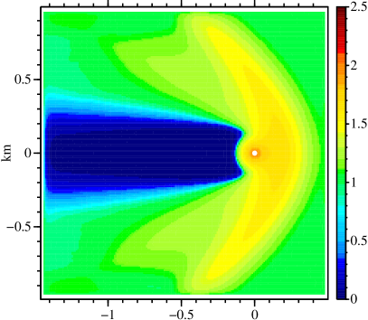
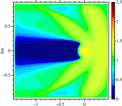
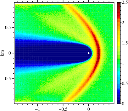
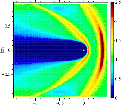
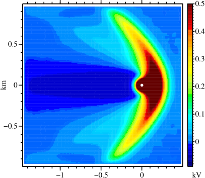
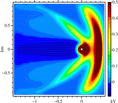
Figure 2: Physically realistic run (left, $\nu=0.12$) and non-physical run (right, $\nu=0.08$) which exhibits double ion deflection shock. The panels are electron density (top), ion density (middle) and electric potential (bottom). Densities are relative to $n_{\rm o}$. White dot shows tether position at the origin.

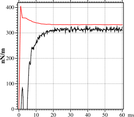
Figure 3: Thrust history in $\nu=0.12$ run: method Mom (black) and method Coul (red).

Table 1: Simulation parameters (high resolution runs). For definition of tether electric radius $r_{w}^{*}$, see Janhunen and Sandroos (2007).

Parameter	Symbol	Value
Grid size		$384\times 384$
Grid spacing	$\Delta x$	$5$ m
$X$ domain		-1.44 .. 0.48 km
$Y$ domain		-0.96 .. 0.96 km
Timestep	$\Delta t$	$2\mu$s
Run duration	$t_{\rm max}$	$60$ ms
Number of timesteps		30000
Ions per cell	$N_{0}$	100 (in plasma stream)
Number of particles		$\sim 15\cdot 10^{6}$
Plasma density	$n_{\rm o}$	$7.3$ cm-3
Ion mass	$m_{i}$	1 amu (protons)
Plasma drift	$v$	400 km/s
Electron temperature	$T_{e}$	10 eV
Ion temperature	$T_{i}$	10 eV
Electron Debye length	$\lambda_{\mathrm{De}}$	8.7 m
Tether voltage	$V_{0}$	$\sim$17.7 kV
Tether electric radius	$r_{w}^{*}$	1 mm
Line charge density	$\lambda$	$8.64\cdot 10^{-8}$ As/m

Table 2: Performed runs. Thrust per tether length in nN/m by Mom and Coul methods, NS=number of shocks. The physically preferred run $\nu=0.12$ is singled out by horizontal lines.

	Low resolution runs			High resolution runs
$\nu$	Mom	Coul	$V_{0}$/kV	Mom	Coul	$V_{0}$/kV	NS	Remarks
0.16	301.1	319.0	17.601	303.6	319.1	17.578	1
0.15	311.5	336.6	17.615	315.6	331.3	17.627	1
0.14	322.3	348.6	17.667	327.3	343.7	17.675	1
0.13	328.1	352.3	17.733	330.1	347.9	17.709	1	Thrust local max
0.12	312.7	340.6	17.745	313.7	332.8	17.725	1	Smallest $\nu$ with NS=1
0.11	296.0	328.5	17.751	300.7	319.8	17.749	1+
0.10	298.7	316.2	17.801	311.7	313.2	17.787	2
0.09	356.5	312.0	17.841	380.9	311.0	17.825	2	Mom$>$Coul
0.08	498.1	308.5	17.881	528.0	307.2	17.868	2	Mom$\gg$Coul