Pixel-wise Segmentation of Street with Neural Networks

Abstract

Pixel-wise street segmentation of photographs taken from a drivers perspective is important for self-driving cars and can also support other object recognition tasks. A framework called SST was developed to examine the accuracy and execution time of different neural networks. The best neural network achieved an $F_{1}$-score of $89.5\text{\,}\frac{\mathrm{\char 37\relax}}{}$ with a simple feedforward neural network which trained to solve a regression task.

I Introduction

Pixel-wise segmentation of street is an important part of assisted and autonomous driving [TB09]. It can help to understand road scenes and reduce the space to search for lane markings. Traditionally, road segmentation is done with computer vision methods such as watershed transformation [BBY90]. Recent advances in deep neural networks, especially in computer vision, suggest that Convolutional Neural Networks (CNNs) might be able to achieve higher classification accuracy on road segmentation tasks then those traditional approaches.

This paper was written in the context of a machine learning hands-on course at Research Center of Information Technology at the KIT (FZI), where self-driving cars are developed. One requirement of self-driving cars is that the algorithms need to be fast (e.g. classify an image in less than $20\text{\,}\frac{\mathrm{ms}}{}$).

Section II mentions published work which influenced us in the choice of our methods. The basics methods used are explained in Section III. It follows a description of the realization in Section IV with a description of the used frameworks as well as details about the developed SST framework. Models are explained in Section V and evaluated in Section VI. Finally, Section VII summarizes the lessons we’ve learned and mentions how our work can be continued.

II Related Work

Road segmentation is a subproblem of general scene parsing or segmentation. In scene parsing every object in a scene is classified pixelwise with a label. Whereas in road segmentation often only two classes exist and more assumptions can be applied.
In the first publications, roads were usually annotated by color-based histogram approaches and specific model knowledge. Examples are the in 1994 introduced approach [BBY90] using the watershed algorithm or [Aly08] where roads were annotated indirectly by lane markings found with a Hough transformation.
Later insights of general scene parsing where transferred and more generic approaches like [GMM12] have achieved remarkable results with a Markov Random Field (MRF) and superpixels.
The impressive classification results of CNNs like AlexNet [KSH12] or GoogLeNet [SLJ⁺14] during the Google ImageNet LSVRC-2010 contest, made CNNs interesting for all kinds of computer vision problems like segmentation.
With [LSD14] Long and his team introduced a method for general scene parsing based on Fully Convolutional Networks (FCNs) and a deconvolutional layer.
This approach is used as a blueprint to our implementation, described in Section V. Therefore the main concepts are introduced in Section III.
Instead of creating a new model, they converted existing classification CNNs like AlexNet or GoogLeNet into FCNs. The obtained heat maps for every class were calculated for multiple resolutions and upscaled with deconvolution layer interpolation to the original resolution. With a fully connected convolutional layer in the end, the multiple outputs are combined into one classification heat map for every class.

In [Moh14] a approach is presented, which makes also use of a CNN in combination with deconvolution. In comparison to Long’s network, among others it is less deep and uses less convolutional then deconvolutional layers. Furthermore the input image is divided in multiple patches and for each patch a separate neural network was trained. Their model achieved the best-recorded result on the same data set we use, which is described in Section VI-A.

III Concept

Two concepts are explained in this section: CNNs and FCNs, which were introduced in [LSD14].

III-A CNN

A CNN is a feedforward neural network with at least one convolutional layer. In general, applying a function repeatedly over the output of other functions is defined as a convolution. In context of CNN a convolution layer is a learned filter which is applied at all possible offsets over an input image. The output of the filter can be seen as an abstraction of the input. Convolutional layers are often combined with pooling layers, which extract one single value out of a larger region. Examples for pooling layer functions are the average or max function.
CNN s can be used for classification with a fully connected layer at the end. The upper part of Figure 1 shows such a network for classification. In the example the input image is classified as “tabby cat”, because this class has the highest probability (illustrated as bar chart).

III-B FCN

A CNN which consists only of convolutional or pooling layers is also known as a FCN. By removing fully connected nodes, the network can generate a output for an image with arbitrary size. In [LSD14] this characteristic is used to train a network that produces a classification heat map. In the lower part of Figure 1, a heat map of probabilities for the presence of a “tabby cat” at different image regions is generated from the input image.

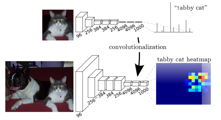
Figure 1: Comparison of a CNN for classification (top) and a FCN which creates a heat map (bottom). The image was taken from [LSD14].

III-C Fully connected convolutional layer

A fully connected convolutional layer is a regular convolutional layer in size of the input. Consequentially, the weight matrix covers every input neuron. Long noted in [LSD14] that it is the two-dimensional equivalent to a fully connected layer in a classification CNN.

III-D Deconvolutional Layer

Deconvolutions are inverse convolutions. In context of neural networks the function for forward and backward calculation are just switched. It is often combined with unpooling and allows to learn how to reconstruct a larger image region from a smaller input. Long indicates in [LSD14] its similarity to interpolation. He explains it as a highly parametrized non-linear interpolation.

IV Realization

IV-A Existing Frameworks

nolearn was used in combination with Lasagne [DSR⁺15] to train the models. Lasagne is based on Theano [BBB⁺10]. We also used Caffe [JSD⁺14] for CNNs, but skipped that approach as the framework crashed very often for different training approaches without giving meaningful error messages.

Theano is a Python package which allows symbolic computation of derivatives as well as automatic generation of GPU code. This is used to calculate the weight update function for arbitrary feed-forward networks. Lasagne makes using Theano simpler by providing basic layer types like fully connected layers, convolutional layers and pooling layers with their update function. nolearn adds syntactic sugar and neural network objects with a similar interface as the scikit-learn package uses for its classifiers [PVG⁺11].

IV-B SST

Street segmentation toolkit (sst) is a Python package hosted on Python Package Index (PyPI) and developed on GitHub. It makes use of Lasagne (see Section IV-A). It was mainly developed during the course “Machine Learning Laboratory — Applications” at KIT by Sebastian Bittel, Vitali Kaiser, Marvin Teichmann and Martin Thoma.

IV-B1 Installation

sst can be installed via pip install sst. To make the installation as simple as possible, this does not try to install all requirements. sst selfcheck gives the user the possibility to check which packages are still required and manually install them.

IV-B2 Functionality

sst makes use of Python files for neural network definitions. Those models must have a generate_nnet(feature_vectors) function which returns an object with a fit(features, labels) method, a predict(feature_vector) method and a predict_proba(feature_vector) method. This is typically achieved by returning a nolearn model object. The Python network definition file has to have two global variables: patch_size (a positive integer) and fully (a Boolean). The first variable is the patch size expected by the neural network, the second variable indicates if the neural network was trained to classify each pixel of the complete patch (fully = True) or only the center pixel (fully = False).

sst --help shows all subcommands. The subcommands are currently

• selfcheck: Test which components or Python packages are missing and have to be installed to be able to use all features of sst.

• train: Train a neural network.

• eval: Evaluate a trained network on a photograph and also generate an overlay image of the segmentation and the data photograph.

• serve: Start a web server which lets the user choose images from the local file system to predict the label and to show overlays.

• view: Show all information about an existing model.

• video: Generate a video.

V Used models

We have implemented two approaches to tackle the street segmentation problem. We have used a sliding window approach which is based on a classification network and a regression approach. Both models are detailed in the following section.

V-A The Sliding Window Approach

Traditionally neural networks are used for classification tasks. As described in Section II they deliver impressive results. Our first approach is a sliding window model, which exploits the classification strength of deep neural networks.

V-A1 Definition of the Classification Problem

We trained a neural network to solve the following binary classification problem:

Classification Problem Input: A $n\times n$ 3-channel pixel image section. Output: Decide whether the center pixel is street.

For $n$ we used $51$. This constant was chosen as we ran into GPU memory problems when training on higher values of $n$. Our classification approach is visualized in Figure 2.

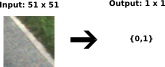
Figure 2: Visualization of the classification problem solved by our neural network.

V-A2 Net Topology

The problem defined above can be tackled with any of the well known classification networks such as GoogLeNet or AlexNet. For our solution we designed our own network detailed in Table I. The small size of only three hidden layers was chosen as our experiments showed that small networks perform better than networks with more layers. One reason for this is that the amount of labeled images is rather small. Hence smaller nets generalize much better. Secondly, the binary decision task of recognizing street is much simpler than detailed image classification. This simplicity does also reflect in the net topology.

Layer	Type	Shape
0	Input	$51\times 51\times 3$
1	Convolution	10 filter each $5\times 5$
2	Convolution	10 filter each $5\times 5$
3	Pooling	$2\times 2$
4	Output	$1$

Table I: Topology of the classification network.

V-A3 Training

The training data for this classification problem can be easily obtained by modifying the original training data. One advantage of our approach is that we get a lot of training data out of each image. In theory, we get one (distinct) datum for each pixel in each training image. However, it is not useful to actually use all of this data as patches which are close to each other and thus are very similar. Hence the information gain of including these patches is very small. On the other hand, if we generate an image section for each pixel we obtain more data than the memory of our GPU can handle. We therefore introduced a training stride. A stride of $s$ results in the center pixels having a distance of $s$ in height and with to the next sections center pixel. This is important in the section generation step before training as well as for the pixel-wise classification. The overlap of two adjacent images is hence reduced to $n-s$, where $n\times n$ is the size of each image section. Empirical evaluations indicated that $s=10$ is a good default value for the trainings stride.

V-A4 Evaluation

In order to apply a classification network on the segmentation problem we used the well known sliding window approach. The main idea is to apply the classification network on each pixel $p$ of the input image by generating the $n\times n$ image section with center pixel $p$. We use padding to be able to apply the method to pixels close to the border. Figure 3 shows the result of this approach.

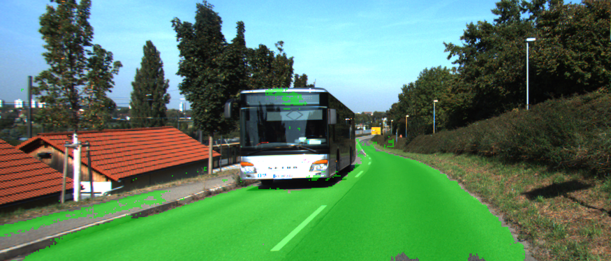
Figure 3: Using the sliding window approach with a stride of $s=2$.

The main disadvantage of this approach is the impractical runtime. For a 1 megapixel image we need to run 1 million classifications. This leads to a runtime of almost two minutes with our hardware. In order to reduce the evaluation time we introduced an evaluation stride $s$. Similar to the training stride we skip $s-1$ pixels in each dimension. This increases the evaluation speed by a factor of $s^{2}$. For the sliding window approach we found that a stride of $s=10$ is a reasonable trade-off between speed and quality. Figure 4 shows the result of the sliding window approach with a stride of $s=10$.

Figure 4: Using the sliding window approach with a stride of $s=10$.

V-B The Regression Approach

The main disadvantage of our sliding window approach is that the segmentation becomes very coarse with higher values for the stride $s$. To overcome this problem we designed a regression neural networks which is able to classify each pixel independently.

V-B1 Definition of the Regression Problem

We trained a neural network to solve the following regression problem:

Regression Problem Input: A $n\times n$ 3-channel pixel image section. Output: A $n\times n$ label.

where the net is trained to minimize the mean squared error of the output. The output of the regression net is continuous. We round the output to obtain a binary classification. Figure 5 visualizes our regression approach.

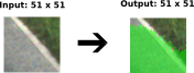
Figure 5: Visualization of the regression approach.

The goal is to choose $n$ as big as possible as $n^{2}$ is the number of pixels which can be classified at once. However, due to GPU memory limitations we cannot train a network with $n>51$.

V-B2 Net Topology

Similar to the classification approach our experiments show that a simple net topologies work best. The topology we used is detailed in Table II.

Layer	Type	Shape
0	Input	$51\times 51\times 3$
1	Convolution	10 filter each $5\times 5$
2	Convolution	1 filter $51\times 51$
3	Reshape (Flatten)	$51\times 51$
4	Output	$2601\times 1$

Table II: Topology of the regression network.

V-B3 Training

Training of the regression model can be implemented analogously to the classification model. We use overlapping image section again to get as much information out of the data as possible.

V-B4 Evaluation

In order to evaluate a whole image using the regression approach we divide the image into patches of size $n\times n$ and evaluate each patch individually. The output is shown in Figure 6. The result is quite impressive, especially regarding the overall runtime of about $0.18\text{\,}\frac{\mathrm{s}}{}$ as shown in Table IV.

Figure 6: Using regression approach with stride $s=51$

One observation is, that the segmentation works better in the center of each patch. The neural network does not have good information close to the border of each image section. To overcome this problem we use an evaluation stride again. This introduces an overlap between each image patch. A pixel $p$ is then segmented according to the patch whose center is closer to $p$.

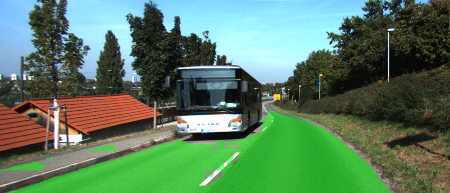
Figure 7: Using regression approach with stride $s=37$

Figure 7 shows the output when using a stride of 37. We see that the edge of the street is classified slightly better. In order to archive this effect a rather big stride between 37 and 47 is already sufficient. In the regression approach there is no measurable benefit of using strides below 37.

VI Experimental Results

In this section we discuss the experimental results of the models presented in Section V. First, we evaluate the two different models. Second, we compare our best one to the work of Mohan [TB09] (which is ranked on place 1 at KITTI road segmentation [TB09]).

VI-A Data Sets

The KITTI Road Estimation data set [FKG13] was used for training of the models and for obtaining the experimental results reported in Section VI.

The left color image base kit contains a training and a test set. All photos are in an urban environment. The training set has 95 photos with land markings (um), 96 photos with multiple lane markings (umm) and 98 photos where the street has no lane markings (uu). The test set has 96 um photos, 94 umm photos and 100 uu photos.

The width of all photos is in $\Set{1226,1238,1241,1242}$, the height is in $\Set{370,374,375,376}$.

The data photos are given as 8-bit color RGB PNG files. The labels (ground truth) are given as images of the same size as the data image, but with only three colors: red (#ff0000), magenta (#ff00ff) for street and black (#000000) for other streets than the one the car is on.

VI-B Metrics / Experiments

For the evaluation of the following experiments we used these metrics: accuracy ($\mathbf{ACC}$), average precision ($\mathbf{AP}$), precision ($\mathbf{PRE}$), recall ($\mathbf{REC}$), false positive rate ($\mathbf{FPR}$), false negative rate ($\mathbf{FNR}$) and the $F_{1}$-measure ($\mathbf{F_{1}}$), see Eqs. 1 to 7. Those metrics make use of true positive (TP), true negative (TN), false positive (FP) and false negative (FN).

(1) ACC $$=\frac{TP+TN}{TP+FP+TN+FN}$$

(2) PRE $$=\frac{TP}{TP+FP}$$

(3) REC $$=\frac{TP}{TP+FN}$$

(4) FPR $$=\frac{FP}{FP+TN}$$

(5) FNR $$=\frac{FN}{TP+FN}$$

(6) AP $$=\frac{1}{11}\displaystyle\sum_{r\in 0,0.1,\dots 1}\max_{\tilde{r}:\tilde{r}>r}\text{Precision}(\tilde{r})$$

(7) $$F_{1} =\frac{2\cdot TP}{2TP+FP+FN}$$

In Eq. 6 $\text{Precision}(\tilde{r})$ is the measured precision at recall $\tilde{r}$ [EVGW⁺10]. These metrics are also used by the official KITTI evaluation.
To be able to evaluate different approaches we used only the training data of the KITTI data set, as the ground truth for the test data is not publicly available. We splitted the training data beforehand 20 to 80 (test/training) in order to be able to measure our performance. Our best model was submitted for the official KITTI evaluation (www.cvlibs.net/datasets/kitti/eval_road.php)

Our goal was to achieve an adequate classification performance while staying within a time frame of $20\text{\,}\frac{\mathrm{ms}}{}$ as maximal classification time per image. As the normal use case of road segmentation would be in autonomous cars the real-time ability is a crucial point.

We used a computer with these specifications for the experiments (GPU was used for training and testing):

• Intel(R) Core(TM) i7-4790K CPU @ $4.00\text{\,}\frac{\mathrm{GHz}}{}$

• System memory $16\text{\,}\frac{\mathrm{GiB}}{}$

• GeForce GTX 980 $4\text{\,}\frac{\mathrm{GiB}}{}$ RAM

Table III shows the result of our evaluation and regression approach using the models and parameters as described in Section V. It shows clearly that the regression model has an overall better $F_{1}$-measure and accuracy score than the classification model. Surprisingly, a smaller stride does not automatically lead to better performance. The classification model shows the best result with a stride of $s=37$, while in the regression based approach a stride $s=51$ achieves the best performance. Unfortunately the RAM of the graphic card limited our possibility to use larger strides and patch sizes. This could have been a promising possibility to train and evaluate on a full image size and still keep our time constraint and even enhance our performance.

Model	$\mathbf{F_{1}}$	TN	FP	FN	TP	ACC
Reg., $s=10$	$88.0\text{\,}\frac{\mathrm{\char 37\relax}}{}$	$97.8\text{\,}\frac{\mathrm{\char 37\relax}}{}$	$2.2\text{\,}\frac{\mathrm{\char 37\relax}}{}$	$19.7\text{\,}\frac{\mathrm{\char 37\relax}}{}$	$80.2\text{\,}\frac{\mathrm{\char 37\relax}}{}$	$94.7\text{\,}\frac{\mathrm{\char 37\relax}}{}$
Reg., $s=37$	$89.0\text{\,}\frac{\mathrm{\char 37\relax}}{}$	$97.3\text{\,}\frac{\mathrm{\char 37\relax}}{}$	$2.6\text{\,}\frac{\mathrm{\char 37\relax}}{}$	$17.6\text{\,}\frac{\mathrm{\char 37\relax}}{}$	$82.3\text{\,}\frac{\mathrm{\char 37\relax}}{}$	$94.8\text{\,}\frac{\mathrm{\char 37\relax}}{}$
Reg., $s=51$	$89.5\text{\,}\frac{\mathrm{\char 37\relax}}{}$	$96.9\text{\,}\frac{\mathrm{\char 37\relax}}{}$	$3.1\text{\,}\frac{\mathrm{\char 37\relax}}{}$	$16.5\text{\,}\frac{\mathrm{\char 37\relax}}{}$	$83.5\text{\,}\frac{\mathrm{\char 37\relax}}{}$	$94.6\text{\,}\frac{\mathrm{\char 37\relax}}{}$
Cla., $s=10$	$85.4\text{\,}\frac{\mathrm{\char 37\relax}}{}$	$98.1\text{\,}\frac{\mathrm{\char 37\relax}}{}$	$1.9\text{\,}\frac{\mathrm{\char 37\relax}}{}$	$24.1\text{\,}\frac{\mathrm{\char 37\relax}}{}$	$75.8\text{\,}\frac{\mathrm{\char 37\relax}}{}$	$94.2\text{\,}\frac{\mathrm{\char 37\relax}}{}$
Cla., $s=37$	$86.2\text{\,}\frac{\mathrm{\char 37\relax}}{}$	$95.9\text{\,}\frac{\mathrm{\char 37\relax}}{}$	$4.1\text{\,}\frac{\mathrm{\char 37\relax}}{}$	$21.2\text{\,}\frac{\mathrm{\char 37\relax}}{}$	$78.7\text{\,}\frac{\mathrm{\char 37\relax}}{}$	$92.9\text{\,}\frac{\mathrm{\char 37\relax}}{}$
Cla., $s=51$	$70.1\text{\,}\frac{\mathrm{\char 37\relax}}{}$	$98.2\text{\,}\frac{\mathrm{\char 37\relax}}{}$	$1.8\text{\,}\frac{\mathrm{\char 37\relax}}{}$	$45.1\text{\,}\frac{\mathrm{\char 37\relax}}{}$	$54.9\text{\,}\frac{\mathrm{\char 37\relax}}{}$	$90.6\text{\,}\frac{\mathrm{\char 37\relax}}{}$

Table III: Results of classification (cla.) and regression (reg.) models with different strides $s$ on our own test set (58 images, $\leavevmode\nobreak\ 6.7\cdot 10^{6}$ pixels). The table entries highlighted in red are the best evaluation scores regarding different parameterizations.

The predefined time constraint (classification of one image in under $20\text{\,}\frac{\mathrm{ms}}{}$) was met which is shown by the run time evaluation displayed in Table IV. As expected, the runtime increases with a smaller stride size. The classification model shows an overall faster run time performance as the regression. Finally, we meet the time constraint by using a stride of $s=51$ in both approaches.

network type / stride $\bm{s}$	10	37	51
regression	$1.99\text{\,}\frac{\mathrm{s}}{}$	$0.29\text{\,}\frac{\mathrm{s}}{}$	$0.18\text{\,}\frac{\mathrm{s}}{}$
classification	$1.83\text{\,}\frac{\mathrm{s}}{}$	$0.20\text{\,}\frac{\mathrm{s}}{}$	$0.11\text{\,}\frac{\mathrm{s}}{}$

Table IV: Runtime per image ($621\times 188$ pixel).

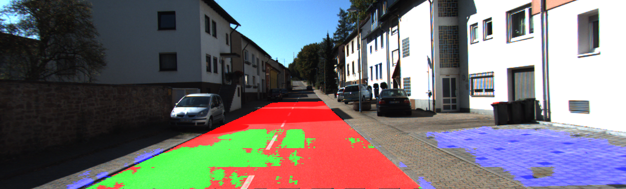
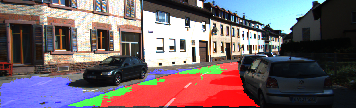
(a) KITTI test data on which our neural net performed badly. Here, red denotes false negatives, blue areas correspond to false positives and green represents true positives.

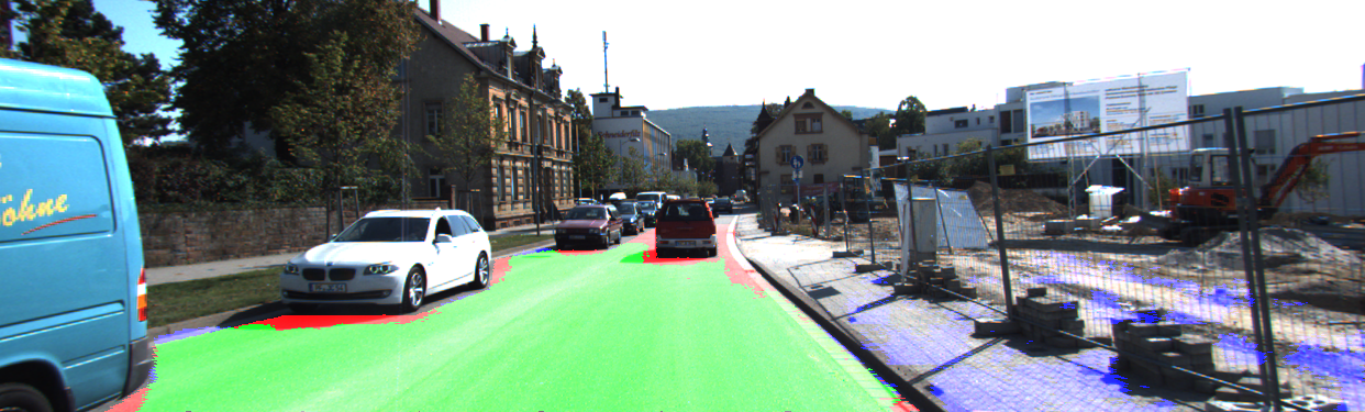
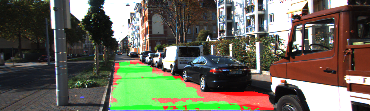
(b) KITTI test data on which our neural net performed well.

Benchmark	$\mathbf{F_{1}}$	AP	PRE	REC	FPR	FNR
UM	$67.91\text{\,}\frac{\mathrm{\char 37\relax}}{}$	$61.63\text{\,}\frac{\mathrm{\char 37\relax}}{}$	$86.90\text{\,}\frac{\mathrm{\char 37\relax}}{}$	$55.74\text{\,}\frac{\mathrm{\char 37\relax}}{}$	$3.83\text{\,}\frac{\mathrm{\char 37\relax}}{}$	$44.26\text{\,}\frac{\mathrm{\char 37\relax}}{}$
UMM	$79.67\text{\,}\frac{\mathrm{\char 37\relax}}{}$	$78.41\text{\,}\frac{\mathrm{\char 37\relax}}{}$	$93.29\text{\,}\frac{\mathrm{\char 37\relax}}{}$	$69.51\text{\,}\frac{\mathrm{\char 37\relax}}{}$	$5.50\text{\,}\frac{\mathrm{\char 37\relax}}{}$	$30.49\text{\,}\frac{\mathrm{\char 37\relax}}{}$
UU	$56.48\text{\,}\frac{\mathrm{\char 37\relax}}{}$	$51.89\text{\,}\frac{\mathrm{\char 37\relax}}{}$	$84.67\text{\,}\frac{\mathrm{\char 37\relax}}{}$	$42.37\text{\,}\frac{\mathrm{\char 37\relax}}{}$	$2.50\text{\,}\frac{\mathrm{\char 37\relax}}{}$	$57.63\text{\,}\frac{\mathrm{\char 37\relax}}{}$
URBAN	$71.10\text{\,}\frac{\mathrm{\char 37\relax}}{}$	$65.14\text{\,}\frac{\mathrm{\char 37\relax}}{}$	$89.83\text{\,}\frac{\mathrm{\char 37\relax}}{}$	$58.84\text{\,}\frac{\mathrm{\char 37\relax}}{}$	$3.67\text{\,}\frac{\mathrm{\char 37\relax}}{}$	$41.16\text{\,}\frac{\mathrm{\char 37\relax}}{}$

Table V: Results of our regression model (stride 51) on the official KITTI evaluation with different road types.

As the regression approach had the best performance and also met our time constraint, we used it to evaluate the KITTI test set and submitted the results after a transformation into birds eye view (KITTI specifications).Table V shows the results which are split into the different road types (UM, UMM, UU, URBAN). Unfortunately, our regression model performs much worse on the official test set than on our own test set. Here the $F_{1}$-measure score ranges between $56.4\text{\,}\frac{\mathrm{\char 37\relax}}{}$ and $79.7\text{\,}\frac{\mathrm{\char 37\relax}}{}$ while Mohan  [TB09] achieves on all road categories a $F_{1}$-measure score of about $90.0\text{\,}\frac{\mathrm{\char 37\relax}}{}$. The reason for this huge difference might be:

1. Overfitting of the neural network on our own test data

2. Specialization of our two models on images with half the original size (the KITTI evaluation is done on full size images)

3. Visible in the two images of Figure 8(a) is an example of very bad performance on a part of the test image data. Basically more non-street is classified as street and most of the street is not recognized as one at all. This could be due to the fact of shadows in some parts of the street and a bit different color of this particular street than most of the street our neural network has learned in the training.

To improve the latter it would be essential to use training data of a lot more different street types and lighting conditions.
Finally Figure 8(b) gives some positives example where our neural network did well. There are hardly no false positives and the street around the cars is nicely segmented.

VII Conclusion

The results presented in this paper were obtained over five months in a hands-on course. We started with the Caffe framework and experimented with a fork created by Jonathan Long. The model he provided could not be used on our computers, because $4\text{\,}\frac{\mathrm{GiB}}{}$ of GPU RAM were not enough to evaluate the model. We tried to adjust the model model, but we failed due to the lack of documentation, cryptic error messages and random crashes while training or evaluating. This was the reason why we switched to Lasagne. Using this framework, we noticed that we still need to try many different topologies. Our first tries lead to bad classification accuracy and we are not aware of any analytical way to determine a network topology for a given task. For this reason, we developed the SST framework. This allows developers to quickly train, test, and evaluate new network topologies. Although the framework got its final flexible form in the last month of the practical course, we used it to evaluate regression and classification models with several topologies. The results are described in Section VI.

In standard scenes, the classification accuracy is impressive. The street gets segmented very well in a runtime of well below $0.5\text{\,}\frac{\mathrm{s}}{}$. However, in some images the model does perform very badly. These are mainly images with special situations such as an uncommon street colors or unusual lightning. We believe that these problems can be easily eliminated by using more training data. Another approach to get better results on the KITTI data set is to train the model with different data and only use the KITTI training data for fine-tuning.

One advantage of our models is that they are perfectly parallelizable. Each image section can be evaluated independently. This can be advantageous in practical applications. When using specialized hardware such as neuromorphic chips it is possible to build hundreds of cores in a car. In such a case our classification approach can yield outstanding results. Given enough training data (e.g. 1.2 million images) using GoogLeNet or AlexNet can provide perfect classification results.

Finally one can also improve the results with better hardware. For some of our models the graphics processing unit (GPU) RAM was the limiting factor. Especially for the regression model using a bigger section of the image can lead to much better results in quality as well as in speed.

References

- [Aly08] M. Aly, “Real time detection of lane markers in urban streets,” in Intelligent Vehicles Symposium, 2008 IEEE. IEEE, 2008, pp. 7–12.
- [BBB+10] J. Bergstra, O. Breuleux, F. Bastien, P. Lamblin, R. Pascanu, G. Desjardins, J. Turian, D. Warde-Farley, and Y. Bengio, “Theano: a CPU and GPU math expression compiler,” in Proceedings of the Python for Scientific Computing Conference (SciPy), Jun. 2010, oral Presentation.
- [BBY90] S. Beucher, M. Bilodeau, and X. Yu, “Road segmentation by watershed algorithms,” in PROMETHEUS Workshop, Sophia Antipolis, France, 1990. [Online]. Available: http://citeseerx.ist.psu.edu/viewdoc/summary?doi=10.1.1.22.5731
- [DSR+15] S. Dieleman, J. Schlüter, C. Raffel, E. Olson, S. K. Sønderby, D. Nouri, D. Maturana, M. Thoma, E. Battenberg, J. Kelly, J. D. Fauw, M. Heilman, diogo149, B. McFee, H. Weideman, takacsg84, peterderivaz, Jon, instagibbs, D. K. Rasul, CongLiu, Britefury, and J. Degrave, “Lasagne: First release.” Aug. 2015. [Online]. Available: http://dx.doi.org/10.5281/zenodo.27878
- [EVGW+10] M. Everingham, L. Van Gool, C. K. Williams, J. Winn, and A. Zisserman, “The pascal visual object classes (voc) challenge,” International journal of computer vision, vol. 88, no. 2, pp. 303–338, 2010.
- [FKG13] J. Fritsch, T. Kuehnl, and A. Geiger, “A new performance measure and evaluation benchmark for road detection algorithms,” in International Conference on Intelligent Transportation Systems (ITSC), 2013.
- [GMM12] C. Guo, S. Mita, and D. McAllester, “Robust road detection and tracking in challenging scenarios based on markov random fields with unsupervised learning,” Intelligent Transportation Systems, IEEE Transactions on, vol. 13, no. 3, pp. 1338–1354, Sept 2012.
- [JSD+14] Y. Jia, E. Shelhamer, J. Donahue, S. Karayev, J. Long, R. Girshick, S. Guadarrama, and T. Darrell, “Caffe: Convolutional architecture for fast feature embedding,” arXiv preprint arXiv:1408.5093, 2014.
- [KSH12] A. Krizhevsky, I. Sutskever, and G. E. Hinton, “Imagenet classification with deep convolutional neural networks,” in Advances in neural information processing systems, 2012, pp. 1097–1105.
- [LSD14] J. Long, E. Shelhamer, and T. Darrell, “Fully convolutional networks for semantic segmentation,” arXiv preprint arXiv:1411.4038, 2014.
- [Moh14] R. Mohan, “Deep deconvolutional networks for scene parsing,” arXiv preprint arXiv:1411.4101, 2014.
- [PVG+11] F. Pedregosa, G. Varoquaux, A. Gramfort, V. Michel, B. Thirion, O. Grisel, M. Blondel, P. Prettenhofer, R. Weiss, V. Dubourg, J. Vanderplas, A. Passos, D. Cournapeau, M. Brucher, M. Perrot, and E. Duchesnay, “Scikit-learn: Machine learning in Python,” Journal of Machine Learning Research, vol. 12, pp. 2825–2830, 2011.
- [SLJ+14] C. Szegedy, W. Liu, Y. Jia, P. Sermanet, S. Reed, D. Anguelov, D. Erhan, V. Vanhoucke, and A. Rabinovich, “Going deeper with convolutions,” CoRR, vol. abs/1409.4842, 2014. [Online]. Available: http://arxiv.org/abs/1409.4842
- [TB09] J.-P. Tarel and E. Bigorgne, “Long-range road detection for off-line scene analysis,” in Intelligent Vehicles Symposium, 2009 IEEE, June 2009, pp. 15–20. [Online]. Available: http://ieeexplore.ieee.org/xpl/login.jsp?tp=&arnumber=5164245&url=http%3A%2F%2Fieeexplore.ieee.org%2Fxpls%2Fabs_all.jsp%3Farnumber%3D5164245