Mg ii Lines Observed during the X-class Flare on 29 March 2014 by the Interface Region Imaging Spectrograph

Abstract

Mg ii lines represent one of the strongest emissions from the chromospheric plasma during solar flares. In this article, we studied the Mg ii lines observed during the X1 flare on March 29 2014 (SOL2014-03-29T17:48) by the Interface Region Imaging Spectrograph (IRIS). IRIS detected large intensity enhancements of the Mg ii h and k lines, subordinate triplet lines, and several other metallic lines at the flare footpoints during this flare. We have used the advantage of the slit-scanning mode (rastering) of IRIS and performed, for the first time, a detailed analysis of spatial and temporal variations of the spectra. Moreover, we were also able to identify positions of strongest hard X-ray (HXR) emissions using the Reuven Ramaty High Energy Solar Spectroscopic Imager (RHESSI) observations and to correlate them with the spatial and temporal evolution of IRIS Mg ii spectra. The light curves of the Mg ii lines increase and peak contemporarily with the HXR emissions but decay more gradually. There are large red asymmetries in the Mg ii h and k lines after the flare peak. We see two spatially well separated groups of Mg ii line profiles, non-reversed and reversed. In some cases, the Mg ii footpoints with reversed profiles are correlated with HXR sources. We show the spatial and temporal behavior of several other line parameters (line metrics) and briefly discuss them. Finally, we have synthesized the Mg ii k line using our non-LTE code with the Multilevel Accelerated Lambda Iteration (MALI) technique. Two kinds of models are considered, the flare model F2 of Machado et al. (1980, ApJ, 242, 336 ) and the models of Ricchiazzi and Canfield (1983, ApJ, 272, 739, RC). Model F2 reproduces the peak intensity of the unreversed Mg ii k profile at flare maximum but does not account for high wing intensities. On the other hand, the RC models show the sensitivity of Mg ii line intensities to various electron-beam parameters. Our simulations also show that the microturbulence produces a broader line core, while the intense line wings are caused by an enhanced line source function.

1 Introduction

The Interface Region Imaging Spectrograph (IRIS: De Pontieu et al., 2014) was launched in the middle of 2013 and since that time many excellent images and spectra were acquired and analyzed, see e.g. a special issue of Science in 2014 (Vol. 346). Among the targets of IRIS, solar flares represent a new challenge because of the unprecedented spatial resolution achieved in the UV/EUV and potentially high cadence, which allows continuous rastering of the flaring region. Many flares have been already captured by IRIS and some of them are X-class flares. IRIS records spectra in two different wavelength channels: FUV (far-UV) from 1332 Å to 1358 Å and 1389 Å to 1407 Å, and NUV (near-UV) from 2783 Å to 2835 Å. In this article, we concentrate on NUV observations with the objective of studying the behavior of Mg ii lines, which appear very bright during flares. To our knowledge, Before the launch of IRIS, the only comprehensive study of Mg ii lines in a flare was based on the 8th Orbiting Solar Observatory (OSO-8) spectral observations obtained in hydrogen, calcium and magnesium lines by the Laboratoire de Physique Stellaire et Planetaire (LPSP) UV spectrometer (Lemaire, Choucq-Bruston, and Vial, 1984). Six resonance lines were detected and their temporal evolution described: hydrogen L$\alpha$ and L$\beta$, Ca ii H (together with the blending H$\epsilon$ Balmer line) and K lines, and Mg ii h and k resonance lines. During the observed flare, the LPSP spectrometer was also able to detect an enhanced emission in three subordinate (intersystem) Mg ii lines, which have wavelengths around the Mg ii k line and appear as absorption lines in the quiet-Sun (QS) spectrum. With the observations from IRIS, the Mg ii lines during an M class flare was studied in detail by Kerr et al. (2015). They investigated the spatial and temporal behaviour of Mg ii lines and found there were red shifts of line centroids, line broadening, and blue asymmetries in flare ribbons. The formation of Mg ii lines in the QS has been recently thoroughly discussed by Leenaarts et al. (2013), in preparation for the analysis of the new IRIS data. It is interesting to note that, according to Lemaire, Choucq-Bruston, and Vial (1984), both Mg ii h and k integrated line intensities are stronger than the hydrogen L$\alpha$ line during the whole evolution of the flare.

Although the hydrogen lines, and in particular the Lyman and Balmer lines, have been extensively modeled for various flare conditions, including time-dependent models, Mg ii lines are largely unexplored. They have been modeled under the QS conditions (Milkey and Mihalas, 1974; Bocchialini and Gouttebroze, 1996; Uitenbroek, 1997; Leenaarts et al., 2013; Avrett, Landi, and McKillop, 2013), but concerning the flare atmospheres, the only study is that of Avrett, Machado, and Kurucz (1986) who used the well-known semi-empirical flare models of Machado et al. (1980) and synthesized the Mg ii k line intensities emergent from F1, F2 and F3 model atmospheres. Lemaire, Choucq-Bruston, and Vial (1984) used the models F1 and F2 and computed their own synthetic intensities to compare with Mg ii OSO-8 observations.

One of the most spectacular events detected by IRIS was the X1-class flare on 29 March 2014 (Kleint et al., 2015b). Several other ground and space instruments observed this flare. Strong Mg ii emission was already reported by Heinzel and Kleint (2014), who studied the accompanying enhancement of the nearby hydrogen Balmer continuum. In this article we perform a first detailed analysis of Mg ii lines in this flare, using the temporal coverage of the flare from its pre-flare period to the decay phase shortly after the flare maximum. We defined several ‘metrics’ quantities and show how they evolve in time. We also perform non-LTE radiative-transfer modeling using the semi-empirical model F2 (Machado et al., 1980) as a representative atmospheric snapshot of the temperature and density structure and compare our synthetic Mg ii line intensities with IRIS observations. We use the theoretical energy balance models of Ricchiazzi and Canfield (1983) to study how various electron-beam parameters affect the profiles of the Mg ii lines.

2 Observations

sec2

The X1 flare observed on 2014 March 29 occurred in the active region (AR) NOAA 12017. It was observed by IRIS from three hours before the flare to a few minutes after the flare peak with a NUV exposure time of 8.00 s before 17:46:04.78 UT and 2.44 s after 17:46:13.98 UT, and 75 s raster cadence (see Section 2 of Heinzel and Kleint (2014) and Section 2 of Young, Tian, and Jaeggli (2015) for detailed descriptions of IRIS observations of this flare). Light curves of the flare in IRIS 1400 Å and IRIS 2796 Å channels, together with X-ray light curves are plotted in Figure fig:lightcurve. The light curves in 1400 Å and 2796 Å are the total counts of the active region, derived from the IRIS slitjaw images, divided by the exposure time. Figure fig:lightcurve shows that the GOES flux started to rise impulsively at 17:45 UT and peaked at 17:48 UT, while fluxes in 1400 Å, 2796 Å and hard X-rays (HXR) peaked 1 – 3 minutes earlier. Figure fig:lightcurve also shows that during the decay phase of the flare, the light curves in the 1400 Å slitjaw image followed the 25–50 keV HXR fluxes observed by the Reuven Ramaty High Energy Solar Spectroscopic Imager (RHESSI: Lin et al., 2002), while the 2796 Å SJI light curve seems to be slightly delayed and more gradual.

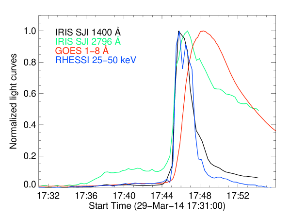
Figure 1.: Normalized and pre-flare subtracted light curves of the 29 March 2014 flare in 1400 Å and 2796 Å (the sum of counts in the images of the AR NOAA 12017 taken by the IRIS slitjaw imager 1400 Å and 2796 Å, divided by the exposure time), in comparison with GOES 1 – 8 Å and RHESSI 25 – 50 keV HXR light curves.fig:lightcurve

  

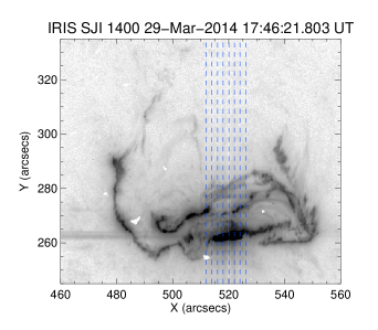
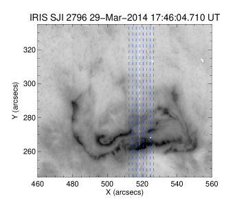
Figure 2.: An IRIS 1400 Å slitjaw image taken at 17:46:22 UT (left) and a 2796 Å slitjaw image at 17:46:04 UT (right), with intensity reversed and in log scale. The IRIS slit positions are indicated by vertical dashed lines.fig:sji

Images of the flare at 17:46 UT in 1400 Å and 2796 Å are presented in Figure fig:sji. The flare ribbons are clearly seen as black patches in the intensity reversed images. Though the contrast of the image in 2796 Å is lower, the flare ribbons look nearly identical in the two images. These images are representative of the plasma in the lower transition region (1400 Å) and upper chromosphere (2796 Å) (De Pontieu et al., 2014). The IRIS slit positions are also plotted in Figure fig:sji as vertical dashed lines; they covered the brightest part of the southern ribbons and part of the northern ribbon during the flare.

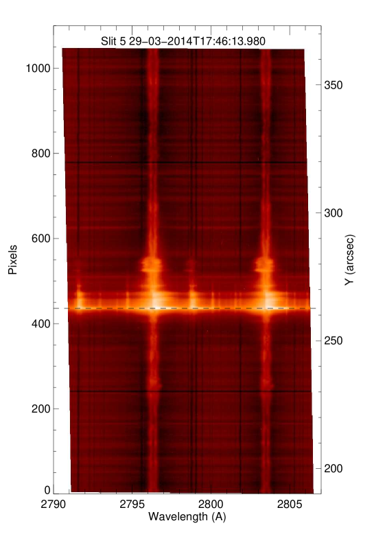
Figure 3.: IRIS spectra of the Mg ii  lines at 17:46:13:98 UT along slit N⁰ 5. The dashed horizontal line indicates the position of pixel 436, which is used to plot the temporal evolution of the line profiles in Figure fig:pixel.fig:spec

Figure fig:spec shows the IRIS spectra of the Mg ii lines taken at 17:46:13.98 UT along slit N⁰ 5. It is clear that there is strong emission in Mg ii h, k, and the subordinate lines, as well as in other metallic lines at 17:46 UT. These emitted Mg ii lines are asymmetric in some of the brightest pixels, with the red wings much broader and brighter than the blue wings. The red asymmetries are usually observed in chromospheric lines (e.g., H$\alpha$, Ca ii K) during flares (e.g., Švestka, Kopecký, and Blaha, 1962; Tang, 1983; Ichimoto and Kurokawa, 1984; Asai et al., 2012; Deng et al., 2013) and are caused by downward motions of the chromospheric material, which is known as chromospheric condensation (Fisher, Canfield, and McClymont, 1985; Fisher, 1989; Longcope, 2014). The dashed horizontal line in Figure fig:spec marks the position of one footpoint pixel, which is the brightest pixel along the slit N⁰ 5 at 17:46:13:98 UT and is used to plot the temporal evolution of Mg ii line profiles in Figure fig:pixel.

We use calibrated IRIS level-2 data. The intensity observed by IRIS in units of data number (DN) is converted to intensities in physical units by the following relation

$$I(\lambda,t)=\frac{n(\lambda,t)~{}Q(\lambda)~{}h~{}c~{}/~{}\lambda}{\delta t~{}\delta\lambda~{}A_{\rm eff}~{}\Omega}\ ,$$ (1)

where $I(\lambda,t)$ is the specific intensity in physical units of erg s^-1 cm^-2 sr^-1 Å^-1, $n(\lambda,t)$ is the observed intensity in units of DN, read from IRIS level-2 data, $\mathbf{Q}(\lambda)$ is the product of the CCD gain and the number of photons needed to create one electron-hole pair on the detector, which is 18 photons DN^-1 for the NUV band (De Pontieu et al., 2014), $h$ is the Planck constant in units of erg s, $c$ is the speed of light in units of cm s^-1, $\lambda$ is the wavelength in cm, $\delta t$ is the exposure time, which is 8 s for this flare in the NUV channel before 17:46 UT, $\delta\lambda$ is the spectral resolution, which is 0.02546 Å for the NUV spectra, $A_{\rm eff}$ is the effective area for the NUV band obtained from the SolarSoftware (SSW: Freeland and Handy, 1998) IDL procedure iris_get_response, and $\Omega$ is the solid angle subtended by one pixel in the y axis of the slit. For the Mg ii spectrum between 2790 Å and 2806 Å, the factor to convert DN s^-1 to physical units is in the range of $1.82\times 10^{4}$ to $1.93\times 10^{4}$. The new IRIS calibration by J.-P. Wülser shows that there is an difference of 10% for the calibration.

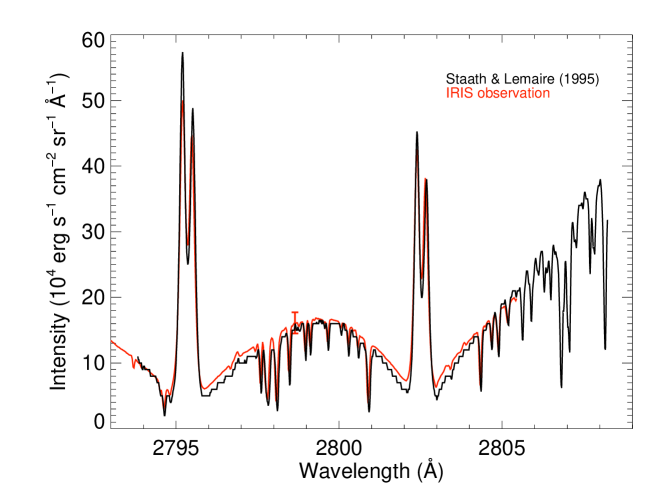
Figure 4.: The Mg ii  spectrum averaged over 100 pixels in the QS region at $\mu=\cos{\theta}$=0.83 in comparison with the QS spectrum observed by RASOLBA at disk center (Staath and Lemaire, 1995). Note that IRIS records spectra in vacuum while the RASOLBA observation was made in the air. We shift the IRIS spectrum by 0.84 Å to the blue to align the wavelengths of these two observations. The error bar in the figure indicates the 10% error for the IRIS calibration.fig:qs

To test the absolute radiometric calibration of the IRIS NUV spectrum, we plot the QS spectrum in the NUV band observed by IRIS in comparison with that observed by the balloon-borne telescope and spectrograph RASOLBA on 19 September 1986 (Staath and Lemaire, 1995) in Figure fig:qs. The IRIS QS spectrum shown in Figure fig:qs is a spectrum averaged over 100 consecutive pixels (pixels 100–199, corresponding to 16.7^′′) and averaged over all eight slit positions in the QS region located at $\mu=\cos{\theta}=0.83$ (Heinzel and Kleint, 2014) taken around 17:30 UT, while the RASOLBA spectrum was an average over 30^′′ slit length and over ten sets of data with alternative 30 s and 90 s exposure times taken at the center of the solar disk. Figure fig:qs shows that the IRIS QS spectrum in the wings of the Mg ii h and k lines is very close to the one from RASOLBA. For example, the IRIS QS spectrum at 2800 Å is 1.62 $\times$ 10⁵ erg s^-1 cm^-2 sr^-1 Å^-1 while the RASOLBA spectrum at the same wavelength is 1.6 $\times$ 10⁵ erg s^-1 cm^-2 sr^-1 Å^-1. The RASOLBA spectrum at 2800 Å is higher than that from the HRTS-9 rocket (Morrill and Korendyke, 2008; Pereira et al., 2013) and other previous calibrated rocket spectra at QS disk center. For example, Kohl and Parkinson (1976) obtained 14.7$\pm$ 1.8, and Bonnet (1968) got 15.0$\pm$3.8 (see Table 2a in Lemaire et al., 1981, for a list of 2800 Å absolute intensity at Sun center). In general, the difference between IRIS and RASOLBA QS spectra in the wings is less than 10% of the RASOLBA data. The differences in the line cores are more pronounced and they reflect the spatial and temporal variations of the quiet chromosphere.

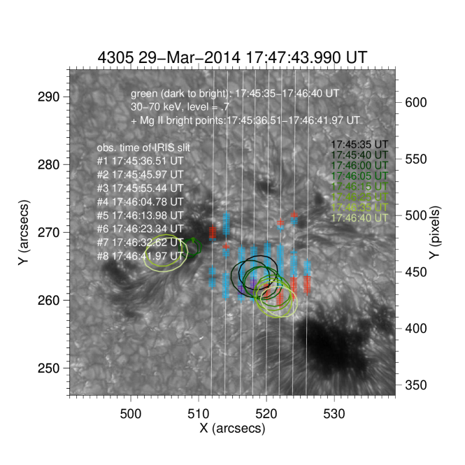
Figure 5.: The Mg ii bright footpoints (with the integrated intensity for the Mg ii h line $\geqslant$ 10⁷ erg s^-1 cm^-2 sr^-1) along all eight slits and RHESSI 30 – 70 keV HXR contours (level = 0.7) overplotted on a G-band image from the Richard B. Dunn Solar Telecope at the National Solar Observatory (NSO/DST). The positions of slits are indicated by vertical white lines. The Mg II bright points are plotted with “+” sign with blue for a non-reversed line profile, red for a reversed line profile, and violet for saturated pixels. The RHESSI contours were created with an integration of 12 s.fig:rhessi

To study the relation between the location of footpoints in Mg ii and HXR sources, we plot the Mg ii bright footpoints along all eight slits for one raster with RHESSI 30 – 70 keV HXR contours around the peak of HXR fluxes in Figure fig:rhessi. We can see that there are two HXR sources around the peak. The IRIS slit did not cross the northern HXR source. The southern HXR source moved south-west and crossed slits 3–7 from 17:45:35 UT to 17:46:40 UT. Mg ii bright footpoints along slits 5 and 6 with reversed profiles coincide well with HXR sources. The Mg ii line profiles at these footpoints become unreversed after the HXR peak, which is clearly seen in the plot of the center-to-peak ratio for slit N⁰ 5 (Figure fig:reversal). Figure fig:rhessi also shows that only a few pixels along slit 3 and 4 (at 17:45:55 UT and 17:46:04 UT, respectively) are saturated in the Mg ii lines. Therefore, the majority of IRIS spectra for this flare are of excellent quality.

In Section sec3, we use several parameters (metrics) to characterize the profiles and intensities of the Mg ii lines and to study their variations during the flare. Since the Mg ii bright footpoints along slits 5 and 6 with reversed profiles are correlated with HXR sources at the HXR peak and the temporal evolution of these metrics along slit 5 and 6 are very similar, we show the evolution of these parameters along slit N⁰ 5 as an example for most cases.

3 Evolution of Mg ii Spectra during the X1 Flare

sec3

Figure fig:pixel shows the temporal evolution of Mg ii spectra in one pixel (pixel 436, slit N⁰ 5) at the footpoint of the flare. The averaged QS spectrum is also plotted in Figure fig:pixel as a reference. Increases of line intensities due to flare energy deposition in the chromosphere are clearly seen in Figure fig:pixel. At the center of the Mg ii h and k lines and the subordinate lines (the three 3p – 3d triplet lines at 2791.6 Å, 2798.8 Å, and 2798.8 Å), intensities increase from 17:36 UT, peak at 17:46 UT and decrease thereafter. At the peak time (17:46 UT), the intensities in the whole spectral range from 2790 Å to 2806 Å increase dramatically, and the widths of the Mg ii lines and metallic lines also increase. Note that for pixel 436 the line profiles of the Mg ii h and k lines are reversed at the peak time and become unreversed after the peak. For pixels close to pixel 436 the Mg ii lines are reversed at the peak time, while for positions a few pixels north of pixel 436 the Mg ii lines are in emission and more symmetric at the peak time. After the peak, the temporal evolution of the line profiles in Mg ii bright pixels along slit N⁰ 5 is similar to that of pixel 436 (line profiles are not shown). At 17:54 UT, the intensities in the wings of the Mg ii h and k lines return to their pre-flare level, which is about 1.5 times the QS intensities. The subordinate lines change from absorption to emission at 17:44 UT and remain in emission after the peak time. All other metallic lines also go into emission at the peak time (17:46 UT) and come back to absorption at 17:54 UT. Figure fig:pixel shows that the line profiles of the h and k lines are very similar and namely the peak intensities are almost the same. Significant red asymmetries of the Mg ii h and k lines are observed at the peak time and after 17:51 UT. Subordinate lines are also significantly asymmetric at the peak time for pixel 436.

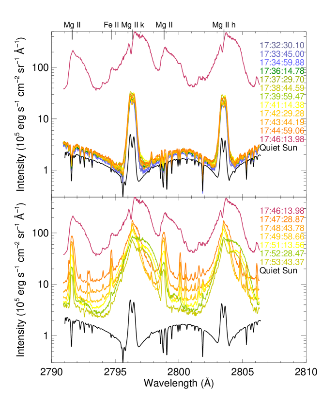
Figure 6.: Temporal evolution of the Mg ii spectra in one pixel (pixel 436, slit N⁰ 5) at the footpoint of the flare. The upper panel shows spectra during the rising phase up to the peak time of Mg ii while the lower panel shows spectra during the decay phase (including the peak time of Mg ii). The QS spectrum is plotted in both panels in black as a reference. The position of the pixel is marked by a dashed horizontal line in Figure fig:spec and in Figure fig:sub-int to fig:fwhm.fig:pixel

The temporal evolution of integrated line intensities for the Mg ii h line over 4 Å along all eight slits from pixel 350 to pixel 600 is plotted in Figure fig:int. Also plotted in these figures are the arbitrarily scaled RHESSI 25 – 50 keV HXR flux in magenta dashed lines and the GOES 1 – 8 Å flux in olive dashed lines. The integrated intensities for the Mg ii h line in Figure fig:int are integrated over a 4 Å band because the h line from the footpoint pixels is very wide with the full width at half maximum (FWHM) around 2 Å after 17:50 UT. Figure fig:int shows that the temporal evolution of integrated Mg ii h line intensities at footpoint pixels along all eight slits is very similar. Bright pixels with an intense Mg ii h line appear when the HXR flux rises impulsively. Then the two ribbons move away from each other: the southern ribbon to the south-west and the northern ribbon to the north. The apparent motion of flare ribbons in the chromosphere may be caused by the flare energy release moving to new coronal loops. Figure fig:int shows that there are also some variations in the integrated intensities for the Mg ii h line at pixels 470–550, which show up before the impulsive phase and continue until the end of the IRIS observations. The penumbra and umbra in slit 7 and slit 8 respectively are also clearly seen in Figure fig:int with low Mg ii h line intensities.

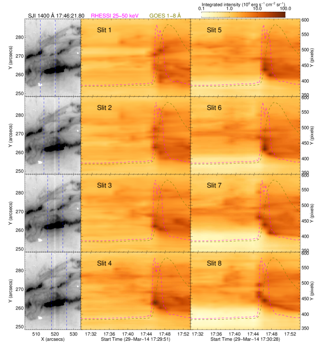
Figure 7.: Left: an IRIS 1400 Å slitjaw image taken at 17:46:21 UT. The vertical dashed lines indicate the positions of the slits which are used to plot the integrated intensity in the center and right columns. Center and right: temporal evolution of the integrated intensities of the Mg ii h line over 4 Å along all eight slits. Arbitrarily scaled RHESSI and GOES light curves are also plotted in the center and right panels. Note that there is a tiny shift in the x axes of the integrated intensity, which is due to a 9 s time step between two consecutive IRIS slit positions.fig:int

Similar to the Mg ii h line, the temporal evolution of subordinate line intensities is very similar at footpoint pixels along all eight slits. As an example, we plot the temporal evolution of integrated line intensities for the subordinate line at 2791.62 Å over 0.53 Å from pixel 350 to pixel 600 along slit N⁰ 5 in Figure fig:sub-int. The Mg ii subordinate lines are in absorption in QS regions and non-flaring active regions. Figure fig:sub-int shows that the subordinate line at 2791.62 Å goes into emission at the footpoint pixels during the flare with integrated intensities peaking at 17:46–17:47 UT. The integrated intensity of the Mg ii subordinate lines at the footpoint pixels rises and peaks as the intensity of the h line, but decreases faster than the h line.

Figure 8.: Temporal evolution of the integrated intensities of the Mg ii subordinate line at 2791.62 Å over 0.53 Å along slit N⁰ 5. The dashed horizontal line indicates the position of pixel 436, which is used to plot the temporal evolution of line profiles in Figure fig:pixel. Arbitrarily scaled RHESSI and GOES light curves are also plotted in the figure.fig:sub-int

As seen in Figure fig:pixel, the metallic lines in the wings of the Mg ii h and k lines at the footpoint pixels also change from absorption to emission during the flare. The temporal evolution of integrated intensities for Fe ii at 2794.69 Å over 0.64 Å along slit N⁰ 5 is plotted in Figure fig:metal-int as an example of those metallic lines. Figure fig:metal-int shows that this line goes into emission at 17:45–17:46 UT and returns to absorption at 17:53:43 UT. Similarly, as for subordinate lines, the integrated intensities for the metallic line also peaks at 17:46–17:47 UT. The metallic line also decreases faster than the Mg ii h line. This may be related to the fact that the Mg ii h and k lines are formed higher in the chromosphere, while the subordinate lines and the iron line are formed much deeper. The temporal evolution of Fe ii (2794.69 Å) intensities at footpoint pixels along other slits is similar to that along slit N⁰ 5 (figures are not shown).

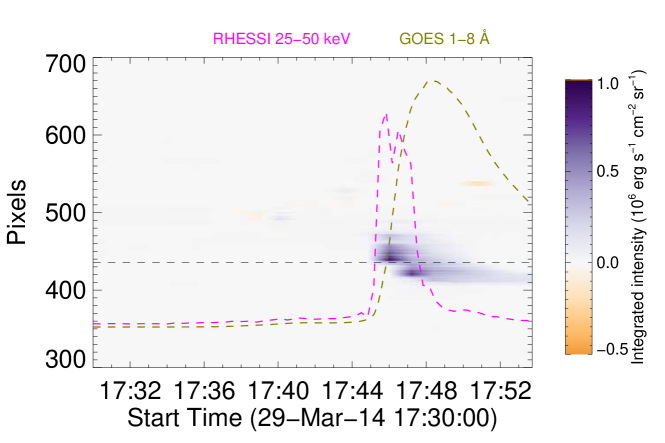
Figure 9.: Temporal evolution of the integrated intensities of Fe ii at 2794.69 Å over 0.64 Å along slit N⁰ 5. The dashed horizontal line indicates the position of pixel 436, which is used to plot the temporal evolution of the line profiles in Figure fig:pixel. Arbitrarily scaled RHESSI and GOES light curves are also plotted in the figure.fig:metal-int

In Figure fig:k2h, we plot the temporal variations of the k to h line ratio, which is the ratio of integrated intensities along slit N⁰ 5 from pixel 350 to pixel 600 which covers the ribbons and part of QS regions. Figure fig:k2h shows that the k to h ratio is in the range between 0.9 to 1.4 along slit N⁰ 5. For pixel 350 to pixel 600 along all eight slits, the k to h ratio is between 0.7 to 1.4. The ratio at footpoint pixels along all eight slits is around 1.1 (with a standard deviation, $\sigma$ = 0.068) and does not change during the flare. This is consistent with previous flare observation by OSO-8/LPSP (Lemaire, Choucq-Bruston, and Vial, 1984) and an M class flare observed by IRIS and analyzed by Kerr et al. (2015), who found the k to h ratio is 1.07 to 1.19 in flaring pixels and does not change much during flare. Figure fig:k2h shows that there are variations of the k to h ratio at pixels 470–550 before the impulsive phase of the flare and during the flare.

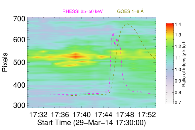
Figure 10.: Ratio of the integrated intensity of the k line to that of the h line along slit N⁰ 5. The dashed horizontal line indicates the position of pixel 436, which is used to plot the temporal evolution of the line profiles in Figure fig:pixel. Arbitrarily scaled RHESSI and GOES light curves are also plotted in the figure.fig:k2h

We use the normalized first-order moment (e.g. Druckmüller, M., Klvaňa, M., and Druckmüllerová, Z., 2007), which is also known as the center of gravity, to measure the centroid of the line

$$\lambda_{g}(\lambda_{0}-\Delta\lambda,\lambda_{0}+\Delta\lambda)=\frac{\int_{\lambda_{0}-\Delta\lambda}^{\lambda_{0}+\Delta\lambda}\lambda\;I(\lambda)~{}{\mathrm{d}}\lambda}{\int_{\lambda_{0}-\Delta\lambda}^{\lambda_{0}+\Delta\lambda}I(\lambda)~{}{\mathrm{d}}\lambda},$$ (2)

where $\lambda_{0}$ is the theoretical line center, $I(\lambda)$ is the intensity at wavelength $\lambda$, $[\lambda_{0}-\Delta\lambda,\lambda_{0}+\Delta\lambda]$ is the interval of integration and $\Delta\lambda$ is estimated as twice the distance between the peak intensity and 1/$e$ of the peak. To reduce the influence of the location of the interval of integration when the observed line is shifted substantially from its theoretical center, the center of gravity is calculated iteratively (Druckmüller, M., Klvaňa, M., and Druckmüllerová, Z., 2007). It is obvious that the center of gravity will move to longer wavelengths if there is a red shift and/or red asymmetry of the line and it will move to shorter wavelengths due to a blue shift and/or blue asymmetry. Therefore, we plot variations of the center of gravity for the Mg ii h line along all eight slits in red and blue colors in Figure fig:lambda-g. We show that the Mg ii h line at footpoint pixels is red shifted and/or red asymmetric when these pixels are bright. The center of gravity for pixels at the northern ribbon is less shifted compared to pixels in the southern ribbon and is only shifted at the time when the pixel is brightest. For most pixels in the southern ribbon, the center of gravity is also shifted to the red wing after 17:49 UT (peak of GOES light curve). The profiles of the Mg ii h line at these footpoint pixels show that the shift is mainly caused by a red asymmetry and therefore the line width is larger at the same time. Figure fig:lambda-g also shows that there are large shifts to the blue at some pixels before the impulsive phase of the flare. Slitjaw images show that the blue shifts and/or blue asymmetries at these pixels are caused by an erupting filament (Kleint et al., 2015b). There are also some small shifts at pixels not related to the filament and flare. Compared to the map of the $k$ to h ratio for slit N⁰ 5 in Figure fig:k2h, these shifts may be related to a larger k to h ratio.

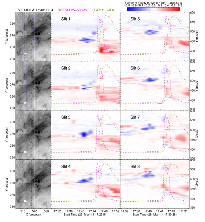
Figure 11.: Left: IRIS 1400 Å slitjaw image taken at 17:40:04 UT. The vertical dashed lines indicate the positions of the slits. For these positions the temporal evolutions of the centers of gravity of the Mg ii h line are plotted in the center and right columns. Arbitrarily scaled RHESSI and GOES light curves are also plotted in the figure. Note that 2803.50 Å is taken as the reference wavelength for plotting the center of gravity because it is the wavelength with the largest number of pixels in the histogram of the center of gravity for all pixels along the eight slits from 17:29:22 UT to 17:54:11 UT. fig:lambda-g

In Figure fig:I-c, we plot the variations of the Mg ii h intensity at its center of gravity along slit N⁰ 5. The variations are mainly at footpoint pixels with intensities increasing at 17:45–17:46 UT and peaking at 17:46–17:47 UT. For other slits, the map of the Mg ii h intensity at its center of gravity also shows clearly when the footpoint pixels start to brighten and become brightest (figures are not shown).

Figure 12.: Mg ii h line intensity at its center of gravity along slit N⁰ 5. The dashed horizontal line indicates the position of pixel 436, which is used to plot the temporal evolution of line profiles in Figure fig:pixel. Arbitrarily scaled RHESSI and GOES light curves are also plotted in the figure.fig:I-c

To describe how much the cores of the Mg ii lines are reversed, we define the center-to-peak ratio as $I_{\rm c}/I_{\rm p}$, where $I_{\rm c}$ is the intensity at the reversal minimum and $I_{\rm p}$ is the intensity at the main peak of the line, which is the maximum intensity of the line. Therefore, the ratio is smaller for line profiles with deeper reversal and larger for line profiles which are less reversed. The ratio value is equal to one for a pure emission line. The variations of this ratio for the Mg ii h line along slit N⁰ 5 are plotted in Figure fig:reversal. We can see that the ratio at some footpoint pixels is close to one, while at other pixels it is about 0.7 (for example, pixel 436, whose profile is shown in Figure fig:pixel). For the filament, the center-to-peak ratio is very small before its eruption and increases when erupting. However, it is interesting to observe a ratio close to one in some active region pixels also before the flare (for example, pixels 380 to 420 and pixels 450 to 470 along slit N⁰ 5).

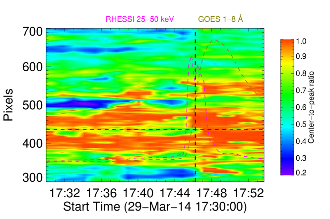
Figure 13.: Center-to-peak ratio of the Mg h line along slit N⁰ 5. The dashed horizontal line indicates the position of pixel 436, which is used to plot the temporal evolution of line profiles in Figure fig:pixel. The vertical dashed line indicates the time 17:46:13:98 UT when the Mg ii bright footpoints along slit N⁰ 5 are plotted in Figure fig:rhessi. Arbitrarily scaled RHESSI and GOES light curves are also plotted in the figure.fig:reversal

To show variations of the line widths during the flare, we plot in Figure fig:fwhm the FWHM of the Mg ii h line along slit N⁰ 5 when it appears as an emission line (i.e. at the time when its center-to-peak ratio is larger than 0.8). We see that the FWHM of the Mg ii h line at the footpoint pixels is larger after 17:50 UT when there are red asymmetries in the line. For this flare, the maximum FWHM of the Mg ii h line is 2 Å which is four times the FWHM at disk center QS regions, where it is observed to be 0.5 $\pm$ 0.02Å (Kohl and Parkinson, 1976; Staath and Lemaire, 1995). Figure fig:fwhm shows that the FWHM of the Mg ii h line in the filament pixels increases two or three minutes before and during the eruption. The shape of a line is also characterized by its various order moments. The line width is expressed in terms of the second order central moment, which is the square of the standard deviation. For an emission line with a Gaussian profile, its FWHM is proportional to its standard deviation.

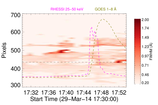
Figure 14.: FWHM of the Mg h line along slit N⁰ 5. The dashed horizontal line indicates the position of pixel 436, which is used to plot the temporal evolution of line profiles in Figure fig:pixel. Arbitrarily scaled RHESSI and GOES light curves are also plotted in the figure.fig:fwhm

Comparing with the flare reported by Lemaire, Choucq-Bruston, and Vial (1984), there are several similarities. First, there are great great emission enhancements in the Mg ii h and k lines and the subordinate lines. Second, the light curves of the Mg ii h or k lines rise and peak at the same time as the subordinate lines. Finally, the $k$ to $h$ ratio is 1.1 $\pm$ 0.068 at footpoint pixels and does not vary with time during the flare. Apart from these similarities, we observe red asymmetries at the flare peak and the decay phase for the X-class flare. Different from the flare of Lemaire, Choucq-Bruston, and Vial (1984), in our flare the light curves of the subordinate lines decrease faster than the light curves of the h and k lines after the peak time. It is interesting to note that some Mg ii line profiles at some footpoint pixels are reversed, while they are non-reversed at other footpoints during the flare, as we have seen before.

4 Synthetic Spectra

sec4

In this section, we present preliminary modeling of the Mg ii lines in a flaring atmosphere to see whether existing flare models can quantitatively reproduce the calibrated IRIS spectra. As we have mentioned in the introduction, the only existing fitting of the Mg ii lines in a flare was performed in Lemaire, Choucq-Bruston, and Vial (1984). We solved the non-LTE radiative-transfer problem to model the Mg ii  lines using a static semi-empirical flare atmosphere. Our numerical code is based on a 1D plane-parallel geometry and assumes the atmosphere in a hydrostatic equilibrium. The non-LTE problem is treated by the so-called Multilevel Accelerated Lambda Iteration (MALI) technique (Rybicki and Hummer, 1991; Heinzel, 1995; Kašparová and Heinzel, 2002). By taking the temperature and pressure structure given by the flare atmosphere, we obtained hydrogen-level populations and electron densities from a five-level plus continuum atomic model of hydrogen. Hydrogen Ly $\alpha$ and Ly $\beta$ lines were treated with the partial frequency redistribution (see Hubeny and Mihalas, 2014). Using the fixed electron density structure, the radiative transfer problem was solved for a five-level plus continuum atomic model of Mg ii with the two resonance lines k and h and the 3p – 3d subordinate triplet around the k line, for details of the atomic model see Heinzel, Vial, and Anzer (2014).

After modeling, we compare our synthetic spectra to the observed IRIS spectra. As the flare was of class X1, we chose the classical semi-empirical flare model F2 of Machado et al. (1980). From an extended grid of synthetic line profiles as shown in Avrett, Machado, and Kurucz (1986) we noticed that the Mg ii k line profile corresponding to model F2 is non-reversed, a feature we observe at several positions. Its peak intensity is quite comparable to that detected around the maximum of Mg ii emission at pixel 447 slit N⁰ 4, just above the saturation region. Using the above mentioned non-LTE technique, we computed the Mg ii line profiles from the F2 model. The resulting Mg ii k line is shown in Figure fig:F2, where we present a few examples for various values of the microturbulent velocity ranging from 0 to 10 km s^-1. Note that this microturbulence is assumed to be uniform in the whole formation region of Mg ii lines, which is certainly a crude approximation. The central line intensities are comparable to the observed ones at about 17:46 UT. The line cores are not much reversed, consistently with the observations. We did not perform a convolution with the IRIS instrumental profile with a width of 52 mÅ; doing so, one could get the emission peaks slightly depressed towards the observed profile (see e.g. Heinzel et al., 2015). The synthetic line profiles are significantly broadened by the microturbulence only in the core, not in the wings. This means that, at least with this schematic model, the observed bright wings are due to an enhanced line source function rather than due to an extra broadening. This can be seen from the formation heights of the Mg ii resonance lines. In Figure fig:cf we show the contribution functions of the Mg ii k line where broad line wings corresponding to the F2 atmosphere are formed over an extended region of about 1000 km. In the quiet Sun, e.g. VAL C atmosphere (Vernazza, Avrett, and Loeser, 1981) which is shown for a comparison, the line wings are formed much deeper in the atmosphere and over a region of only some 200 km wide. Finally, we also tested the influence of the coronal pressure on the line spectrum. Model F2 has an upper boundary gas pressure equal to about 95 dyn cm^-2. The test solution without this pressure leads to a much lower central intensity of the k and h lines. Therefore, the overlying hot loops seem to have an important influence on the line-core emission. The enhanced pressure is related to the explosive evaporation process, described in the next paragraph.

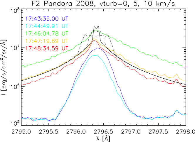
Figure 15.: A comparison between the synthetic Mg ii k line intensities computed from model F2 and IRIS observations for slit N⁰ 4 in pixel 447. The profiles have been obtained for three microturbulent velocities: 0 km s^-1 - full line, 5 km s^-1 - dashed line, and 10 km s^-1 dash-dotted line. ‘Pandora 2008’ is the version of the F2 model with a slightly different coronal pressure from the original model of Machado et al. (1980). Note the intensity decrease at time 17:44:49.91. fig:F2

  

  

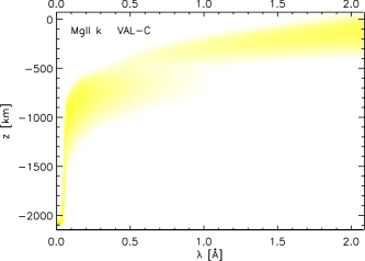
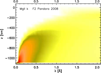
                              (a)                                 (b)

Figure 16.: Mg ii k line contribution function for: (a) VAL C and (b) F2 model atmospheres. Note the height scale $z$ is inverted ($z=0$ denotes photosphere) and it is different for each model. We clearly see how the chromosphere is affected by the heating, contributing significantly to the line wings. The QS wings are formed much deeper.fig:cf

To demonstrate the dependence of Mg ii line intensities and line profile shapes on various model parameters, we have also computed a grid of profiles based on models by Ricchiazzi and Canfield (1983) (hereafter called RC models). Although these models have been published more than three decades ago, they still represent the only systematic grid of theoretical flare models. RC models are 1D static atmosphere models in stationary energy balance where the chromosphere is heated by electron beams. The latter are parameterized by the total energy flux above a low-energy cutoff of 20 keV and a spectral index $\delta$. Another parameter is the coronal pressure at the top of the model atmosphere which is supposed to be enhanced as a result of explosive evaporation. Using RC models, we have computed synthetic Mg ii k line profiles displayed in Figure fig:RC. Figure fig:RCa shows the line-profile variations with increasing electron-beam flux, from 10⁹ to 10¹¹ erg s^-1 cm^-2. The spectral index is equal to five and the coronal pressure is 1 dyn cm^-2. All profiles are rather strongly reversed although for higher fluxes, the averaged line-core intensities are comparable to the observed ones. The wings are however too low. The central line reversal is significantly reduced for higher coronal pressures, as shown in Figure fig:RCb. For the highest value of the pressure, the profile is non-reversed, but its central intensity is much higher compared to observations. Finally, Figure fig:RCc shows how the wing intensities increase with decreasing $\delta$, while the line core remains practically unchanged. At $\delta$=3 the wing reaches the observed intensities, which indicates a deep penetration of the beam into lower atmospheric layers, which are then more heated, contrary to models with a higher $\delta$ or the semi-empirical model F2. From this analysis we can conclude that a model with higher flux, between 10¹⁰ and 10¹¹ erg s^-1 cm^-2, a spectral index around three, and and enhanced coronal pressure between 10 – 100 dyn cm^-2 could roughly reproduce the observations. Such fluxes and spectral indexes are consistent with those derived for this flare from detailed analysis of RHESSI spectra obtained at the same time and locations as the Mg ii spectra reported in this article (Kleint et al., 2015a).

  

                             (a)                                 (b)

  

                                             (c)

Figure 17.: Mg ii k line profiles computed from RC models with different parameters. (a) $\delta$=5, coronal pressure 1 dyn cm^-2 and three electron-beam fluxes 10⁹ (solid line), 10¹⁰ (dashed line) and 10¹¹ erg s^-1 cm^-2 (dash-dotted line). (b) $\delta$=5, flux 10¹⁰ erg s^-1 cm^-2 and four different values of the coronal pressure 1 (solid line), 10 (dashed line), 100 (dash-dotted line) and 1000 dyn cm^-2 (dash-three-dotted line). (c) the electron-beam flux 10¹¹ erg s^-1 cm^-2, coronal pressure 100 dyn cm^-2 and three spectral indexes of the electron beam $\delta$=3 (solid line), $\delta$=5 (dashed line) and $\delta$=7 (dot-dashed line).fig:RC

There is still another aspect to be taken into account when one compares the enhanced wings of the k and h lines. As found by Heinzel and Kleint (2014), there seems to be a rather significant Balmer-continuum emission during the maximum of this flare detected in the NUV channel of IRIS. Assuming that this emission is optically thin in the chromosphere, one can subtract it from the NUV spectrum by using the Lockheed Martin Solar and Astrophysics Laboratory (LMSAL) pre-flight calibration for the IRIS NUV spectra as in Heinzel and Kleint (2014). This is shown in Figure fig:cont, where the Balmer continuum is subtracted from the spectrum at 17:46:04.78 UT (depending on the radiometric calibration used (Heinzel and Kleint, 2014) one gets the continuum levels differing by about a factor of three). The effect of the Balmer continuum is marginal in the line core and inner wings where the line intensity is high, but it is significant in the extended wings. Since our preliminary synthesis of the Mg ii lines does not account for an enhanced Balmer continuum of hydrogen, we should compare the synthetic profiles from Figure fig:F2 with the reduced ones in this Figure fig:cont. This naturally leads to a somewhat better agreement. Note that when calculating the integrated intensities for the subordinate line or metallic line, we subtract the continuum intensities at the wings near the center of the subordinate line or the metallic line before integration. So the integrated intensities in Figure fig:sub-int and Figure fig:metal-int are not affected by the Balmer continuum.

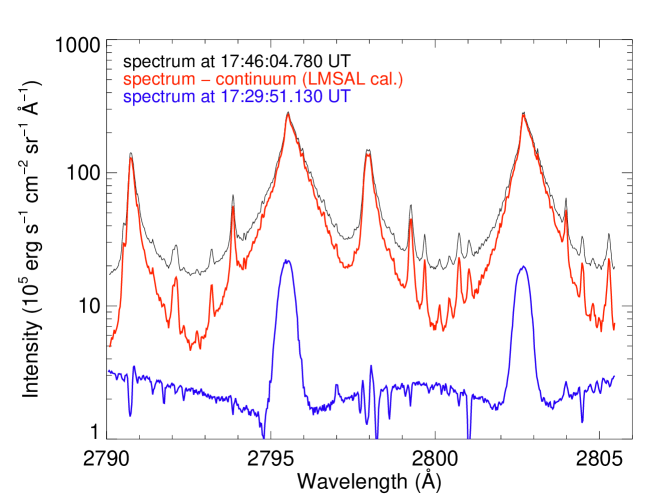
Figure 18.: Observed Mg ii spectrum at 17:46:04.780 UT with (red) and without (black) the Balmer continuum subtracted at pixel 447 slit N⁰ 4. The pre-flare spectrum at pixel 447 is also plotted in the figure with a blue continuous line, as a reference.fig:cont

5 Conclusions

We study the 2D spatial and temporal evolution of flare ribbons in Mg ii lines in detail. The observations of the Mg ii spectrum along all eight slits can be summarized as follows. (1) The intensities of the Mg ii lines at the footpoints increase during the impulsive phase of the flare and peak at the maximum of the HXR emission. (2) The $k$ to $h$ ratio of the integrated intensities is 1.1 $\pm$ 0.068 at the footpoints and does not vary during the flare. (3) There are red asymmetries at most footpoints located in the southern ribbon after the peak. (4) The Mg ii h and k lines are non-reversed at some footpoints and reversed at others at the flare peak. Some of the Mg ii footpoints with reversed profiles are correlated with HXR sources. After the peak, the Mg ii line profiles at most footpoints become non-reversed. (5) The subordinate lines and metallic lines at the footpoints rise from absorption to emission during the flare. (6) The Mg ii lines become broader during the flare.

We have compared the observed line intensities with synthetic spectra computed from the semi-empirical model F2 and found several similarities. The temperature structure of the F2 model, which can be regarded as a ‘snapshot’ of a more realistic model evolution, reproduces some features of the observed profiles, but does not explain the broad line wings well, which will require stronger heating deeper in the chromosphere. Since the original F2 model was constructed without taking into account the non-thermal rates in hydrogen, we also neglected this aspect. For the Mg ii lines, the non-thermal processes seem to be of a secondary importance as we found from several tests. Another class of models is represented by a grid of theoretical flare models constructed by RC. For these models we have synthesized the Mg ii k profiles and shown that for some specific model parameters they roughly fit our observations. However, all used models are static and thus they do not reproduce the line asymmetries observed in some pixels. These mostly red asymmetries are usually associated with the downward moving chromospheric plasma. The velocity field affects the line profiles (asymmetry), but also significantly influences the line intensities via the statistical equilibrium for the Mg ii atom. Without any systematic modeling, it is rather difficult to interpret the observation that the Mg ii line profiles are grouped into reversed (red in Figure fig:rhessi) and non-reversed (blue in Figure fig:rhessi). However, based on a limited grid of RC models, we may speculate that reversed profiles will appear at sites of strong heating and moderate coronal pressures where the chromospheric condensation (downflows) is formed due to the electron-beam impact, leading to the red asymmetries which are observed. On the other hand, unreversed and more symmetrical profiles might be related to higher coronal pressures (the loops are filled with the evaporated plasma) and motions inside the ribbons are very small. This might be consistent with Figure fig:rhessi where the outer edges of the southern ribbon may represent the footpoints of hot loops in which the electron beams propagate, while the inner edges are places where cooler and denser loops are rooted. From the modeling we found that the line cores are very sensitive to gas pressure in overlying coronal loops. In a future study we plan to perform more realistic radiative-hydrodynamical simulations of the temporal evolution of flare spectra using the code Flarix developed at the Ondřejov observatory (Varady et al., 2010). Electron-beam spectra derived from simultaneous RHESSI observations (see Kleint et al., 2015a) will be used. These simulations will also allow us to study the velocity flows, which cause the line asymmetries.

Acknowledgements

The research leading to these results has received funding from the European Community s Seventh Framework Programme (FP7/2007–2013) under grant agreement N⁰ 606862 (F-CHROMA) and from ASI ASCR project RVO:67985815. L.K. was supported by a Marie-Curie Fellowship. IRIS is a NASA small explorer mission developed and operated by LMSAL with mission operation executed at the NASA Ames Research Center and major contributions to downlink communications funded by the Norwegian Space Center (NSC, Norway) through an ESA PRODEX contract.

Disclosure of Potential Conflicts of Interest

The authors declare that they have no conflicts of interest.

References

- Asai et al. (2012) Asai, A., Ichimoto, K., Kita, R., Kurokawa, H., Shibata, K.: 2012, A Study on Red Asymmetry of H Flare Ribbons Using a Narrowband Filtergram in the 2001 April 10 Solar Flare. PASJ 64, 20. DOI. ADS.
- Avrett, Landi, and McKillop (2013) Avrett, E., Landi, E., McKillop, S.: 2013, Calculated Resonance Line Profiles of [Mg II], [C II], and [Si IV] in the Solar Atmosphere. ApJ 779, 155. DOI. ADS.
- Avrett, Machado, and Kurucz (1986) Avrett, E.H., Machado, M.E., Kurucz, R.L.: 1986, Chromospheric flare models. In: Neidig, D.F. (ed.) The lower atmosphere of solar flares, 216. ADS.
- Bocchialini and Gouttebroze (1996) Bocchialini, K., Gouttebroze, P.: 1996, Solar chromospheric structures as observed simultaneously in strong UV lines. II. Network and cell modelling. A&A 313, 949. ADS.
- Bonnet (1968) Bonnet, J.: 1968, Recherches sur l’émission continue du Soelil entre 1950 & Aring et 3000 Å. Ann. d’Astrophysique 31, 597. ADS.
- De Pontieu et al. (2014) De Pontieu, B., Title, A.M., Lemen, J.R., Kushner, G.D., Akin, D.J., Allard, B., et al.: 2014, The Interface Region Imaging Spectrograph (IRIS). Sol. Phys. 289, 2733. DOI. ADS.
- Deng et al. (2013) Deng, N., Tritschler, A., Jing, J., Chen, X., Liu, C., Reardon, K., Denker, C., Xu, Y., Wang, H.: 2013, High-cadence and High-resolution H Imaging Spectroscopy of a Circular Flare’s Remote Ribbon with IBIS. ApJ 769, 112. DOI. ADS.
- Druckmüller, M., Klvaňa, M., and Druckmüllerová, Z. (2007) Druckmüller, M., Klvaňa, M., Druckmüllerová, Z.: 2007, Solar Spectra Analysis Based on the Statistical Moment Method. Central European Astrophys. Bull. 31, 297. ADS.
- Fisher (1989) Fisher, G.H.: 1989, Dynamics of flare-driven chromospheric condensations. ApJ 346, 1019. DOI. ADS.
- Fisher, Canfield, and McClymont (1985) Fisher, G.H., Canfield, R.C., McClymont, A.N.: 1985, Flare Loop Radiative Hydrodynamics - Part Seven - Dynamics of the Thick Target Heated Chromosphere. ApJ 289, 434. DOI. ADS.
- Freeland and Handy (1998) Freeland, S.L., Handy, B.N.: 1998, Data Analysis with the SolarSoft System. Sol. Phys. 182, 497. DOI. ADS.
- Heinzel (1995) Heinzel, P.: 1995, Multilevel NLTE radiative transfer in isolated atmospheric structures: implementation of the MALI-technique. A&A 299, 563. ADS.
- Heinzel and Kleint (2014) Heinzel, P., Kleint, L.: 2014, Hydrogen Balmer Continuum in Solar Flares Detected by the Interface Region Imaging Spectrograph (IRIS). ApJ 794, L23. DOI. ADS.
- Heinzel, Vial, and Anzer (2014) Heinzel, P., Vial, J.-C., Anzer, U.: 2014, On the formation of Mg ii h and k lines in solar prominences. A&A 564, A132. DOI. ADS.
- Heinzel et al. (2015) Heinzel, P., Schmieder, B., Mein, N., Gunár, S.: 2015, Understanding the Mg II and H Spectra in a Highly Dynamical Solar Prominence. ApJ 800, L13. DOI. ADS.
- Hubeny and Mihalas (2014) Hubeny, I., Mihalas, D.: 2014, Theory of Stellar Atmospheres, Princeton Univ. Press, Princeton, New Jersey, USA. ADS.
- Ichimoto and Kurokawa (1984) Ichimoto, K., Kurokawa, H.: 1984, H-alpha red asymmetry of solar flares. Sol. Phys. 93, 105. DOI. ADS.
- Kašparová and Heinzel (2002) Kašparová, J., Heinzel, P.: 2002, Diagnostics of electron bombardment in solar flares from hydrogen Balmer lines. A&A 382, 688. DOI. ADS.
- Kerr et al. (2015) Kerr, G.S., Simões, P.J.A., Qiu, J., Fletcher, L.: 2015, IRIS observations of the Mg ii h and k lines during a solar flare. A&A 582, A50. DOI. ADS.
- Kleint et al. (2015a) Kleint, L., Heinzel, P., Judge, P., Krucker, S.: 2015a, ApJ submitted.
- Kleint et al. (2015b) Kleint, L., Battaglia, M., Reardon, K., Sainz Dalda, A., Young, P.R., Krucker, S.: 2015b, The Fast Filament Eruption Leading to the X-flare on 2014 March 29. ApJ 806, 9. DOI. ADS.
- Kohl and Parkinson (1976) Kohl, J.L., Parkinson, W.H.: 1976, The MG II H and K lines. I - Absolute center and limb measurements of the solar profiles. ApJ 205, 599. DOI. ADS.
- Leenaarts et al. (2013) Leenaarts, J., Pereira, T.M.D., Carlsson, M., Uitenbroek, H., De Pontieu, B.: 2013, The Formation of IRIS Diagnostics. I. A Quintessential Model Atom of Mg II and General Formation Properties of the Mg II h & k Lines. ApJ 772, 89. DOI. ADS.
- Lemaire, Choucq-Bruston, and Vial (1984) Lemaire, P., Choucq-Bruston, M., Vial, J.-C.: 1984, Simultaneous H and K CA II, H and K MG II, L-alpha and L-beta H I profiles of the April 15, 1978 solar flare observed with the OSO-8/L.P.S.P. experiment. Sol. Phys. 90, 63. DOI. ADS.
- Lemaire et al. (1981) Lemaire, P., Gouttebroze, P., Vial, J.C., Artzner, G.E.: 1981, Physical properties of the solar chromosphere deduced from optically thick lines. I - Observations, data reduction, and modelling of an average plage. A&A 103, 160. ADS.
- Lin et al. (2002) Lin, R.P., Dennis, B.R., Hurford, G.J., Smith, D.M., Zehnder, A., Harvey, P.R., et al.: 2002, The Reuven Ramaty High-Energy Solar Spectroscopic Imager (RHESSI). Sol. Phys. 210, 3. DOI. ADS.
- Longcope (2014) Longcope, D.W.: 2014, A Simple Model of Chromospheric Evaporation and Condensation Driven Conductively in a Solar Flare. ApJ 795, 10. DOI. ADS.
- Machado et al. (1980) Machado, M.E., Avrett, E.H., Vernazza, J.E., Noyes, R.W.: 1980, Semiempirical models of chromospheric flare regions. ApJ 242, 336. DOI. ADS.
- Milkey and Mihalas (1974) Milkey, R.W., Mihalas, D.: 1974, Resonance-line transfer with partial redistribution. II - The solar MG II lines. ApJ 192, 769. DOI. ADS.
- Morrill and Korendyke (2008) Morrill, J.S., Korendyke, C.M.: 2008, High-Resolution Center-to-Limb Variation of the Quiet Solar Spectrum near Mg II. ApJ 687, 646. DOI. ADS.
- Pereira et al. (2013) Pereira, T.M.D., Leenaarts, J., De Pontieu, B., Carlsson, M., Uitenbroek, H.: 2013, The Formation of IRIS Diagnostics. III. Near-ultraviolet Spectra and Images. ApJ 778, 143. DOI. ADS.
- Ricchiazzi and Canfield (1983) Ricchiazzi, P.J., Canfield, R.C.: 1983, A static model of chromospheric heating in solar flares. ApJ 272, 739. DOI. ADS.
- Rybicki and Hummer (1991) Rybicki, G.B., Hummer, D.G.: 1991, An accelerated lambda iteration method for multilevel radiative transfer. I - Non-overlapping lines with background continuum. A&A 245, 171. ADS.
- Staath and Lemaire (1995) Staath, E., Lemaire, P.: 1995, High resolution profiles of the MG II H and MG II K lines. A&A 295, 517. ADS.
- Tang (1983) Tang, F.: 1983, Flare asymmetry as seen in offband H-alpha filtergrams. Sol. Phys. 83, 15. DOI. ADS.
- Uitenbroek (1997) Uitenbroek, H.: 1997, THE SOLAR MG II H AND K LINES - Observations and Radiative Transfer Modeling. Sol. Phys. 172, 109. DOI. ADS.
- Švestka, Kopecký, and Blaha (1962) Švestka, Z., Kopecký, M., Blaha, M.: 1962, Qualitative discussion of 244 flare spectra. II. Line asymmetry and helium lines. Bull. Astron. Inst. Czechoslovakia 13, 37. ADS.
- Varady et al. (2010) Varady, M., Kasparova, J., Moravec, Z., Heinzel, P., Karlicky, M.: 2010, Modeling of Solar Flare Plasma and Its Radiation. IEEE Trans. Plasma Scien. 38, 2249. DOI. ADS.
- Vernazza, Avrett, and Loeser (1981) Vernazza, J.E., Avrett, E.H., Loeser, R.: 1981, Structure of the solar chromosphere. III - Models of the EUV brightness components of the quiet-sun. ApJS 45, 635. DOI. ADS.
- Young, Tian, and Jaeggli (2015) Young, P.R., Tian, H., Jaeggli, S.: 2015, The 2014 March 29 X-flare: Subarcsecond Resolution Observations of Fe XXI 1354.1. ApJ 799, 218. DOI. ADS.