Large N meson propagators from twisted space-time reduced model

Abstract:

Recently, we proposed a new method to calculate meson propagators in the large $N$ limit from twisted space-time reduced model. In this note, we give simulation details for obtaining meson spectra and discuss the smearing technique which should improve the signal of meson propagators in future works.

1 Introduction

In the last few years, we have performed several studies of the twisted space-time reduced model. This is a one-site lattice model[1, 2], expected to become equivalent in the large $N$ limit to the usual lattice gauge theory at infinite volume. We have identified the condition on the twisted boundary condition which ensures this equivalence[3]. We have also calculated a variety of quantities on both lattice[4] and continuum[5, 6] space-time. We also showed that it is straightforward to introduce adjoint fermions within our framework[7, 8].

Although one of the most important observables of lattice gauge theories is given by the hadron spectra, our previous studies did not attempt to calculate it in the twisted reduced model. At first sight it seemed impossible to calculate space-time extended hadron correlation functions in the one-site model. Furthermore, the presence of quarks in the fundamental representation of the group seemed in conflict with twisted boundary conditions. Recently, we found a way to circumvent these difficulties and succeeded in calculating meson spectra in the large $N$ limit[9]. The purpose of this note is to present simulation details which are not covered in ref[9], and propose a new smearing method which should be indispensable for a precise determination of meson spectra.

2 Formulation

We consider the twisted Eguchi-Kawai model with gauge group SU($N$) with $N=L^{2}$, $L$ being positive (preferably prime) integer. The action of the TEK model is given by

$$S=-bN\sum_{\mu\neq\nu=0}^{d-1}z_{\nu\mu}{\rm Tr}\left[U_{\mu}U_{\nu}U_{\mu}^{\dagger}U_{\nu}^{\dagger}\right]$$ (1)

Here, $U_{\mu}$ are d=4 SU($N$) link variables. The symmetric twist tensor $z_{\mu\nu}$ is an element of Z($L$);

$$z_{\nu\mu}=\exp\left(k{2\pi i\over L}\right),\ \ \ z_{\mu\nu}=z_{\nu\mu}^{*},\ \ \ \mu>\nu$$ (2)

$k$ and $L$ are co-prime and should obey some constraint in order to avoid Z($N$) symmetry breaking at intermediate values of the coupling[3]. The minimum action solution is given by matrices $\Gamma_{\mu}$ satisfying

$$\Gamma_{\mu}\Gamma_{\nu}=z_{\mu\nu}\Gamma_{\nu}\Gamma_{\mu}$$ (3)

whose explicit form is given, for example, in eq. (2.13) of ref.[4].

As has been shown in ref.[9], the meson propagator in channel $\gamma_{A}$ and $\gamma_{B}$ at time distance $n_{0}$ is given by the following formula

$$C_{AB}(n_{0})={1\over\ell_{0}N^{3/2}}\sum_{q_{0}}{\rm e}^{-iq_{0}n_{0}}{\rm Tr}\left[\gamma_{A}D^{-1}(0)\gamma_{B}D^{-1}(q_{0})\right]$$ (4)

Here $D(q_{0})$ is the Wilson-Dirac matrix acting on color ($U_{\mu}$), spatial ($\Gamma_{\mu}$) and Dirac ($\gamma_{\mu}$) spaces and its explicit form is

$$D(q_{0})=1-\kappa\sum_{\mu=0}^{d-1}\left[(1-\gamma_{\mu}){\tilde{U}_{\mu}}\Gamma_{\mu}^{*}+(1+\gamma_{\mu}){\tilde{U}_{\mu}^{\dagger}}\Gamma_{\mu}^{t}\right]$$ (5)

with

$${\tilde{U}_{\mu=0}}={\rm e}^{iq_{0}}U_{\mu=0},\ \ \ \ \ {\tilde{U}_{\mu=1,2,3}}=U_{\mu=1,2,3}$$ (6)

and

$$q_{0}={2\pi m\over\ell_{0}L},\ \ \ \ 0\leq m\leq\ell_{0}L-1$$ (7)

Quark fields are supposed to live in a finite box $\ell_{0}L\times L^{3}$ with positive integer $\ell_{0}$, whereas gauge fields live in a $L\times L^{3}$. A value of $\ell_{0}>1$ is very convenient since in formula (4) we represent the correlation function of ultralocal meson operators in spatially zero momentum state. This correlator receives important contributions of higher excitation and one must go to relatively long time separation to extract a good signal for the lowest mass state. As will be discussed in sect. 4, this problem can be circumvented by using spatially extended smeared meson operators.

We use $Z(4)$ random source method to compute Tr in (4). Let $z(\alpha,\beta,i)$ be the source vector having color ($U_{\mu}$) index $1\leq\alpha\leq N$, spatial ($\Gamma_{\mu}$) index $1\leq\beta\leq N$ and Dirac ($\gamma_{\mu}$) index $1\leq i\leq 4$. Then $z(\alpha,\beta,i)={1\over\sqrt{2}}(\pm 1\pm i)$. After averaging over random source, we have $\left<z^{*}(\alpha^{\prime},\beta^{\prime},i^{\prime})z(\alpha,\beta,i)\right>=\delta_{\alpha^{\prime}\alpha}\delta_{\beta^{\prime}\beta}\delta_{i^{\prime}i}$. Now we define Hermitian operator $Q(q_{0})=D(q_{0})\gamma_{5}$ and solve the following $\ell_{0}L+1$ equations.

$$Q(0)x_{A}=\gamma_{5}\gamma_{A}^{\dagger}z$$ (8)

$$Q(q_{0})\gamma_{5}\gamma_{B}^{-1}y_{B}(q_{0})=z,\ \ \ \ q_{0}={2\pi m\over\ell_{0}L},\ \ \ \ 0\leq m\leq\ell_{0}L-1$$ (9)

Taking the inner product of $x_{A}^{\dagger}$ and $y_{B}(q_{0})$ and averaging over random source, we have

$$\left<x_{A}^{\dagger}y_{B}(q_{0})\right> = \left<z^{\dagger}\gamma_{A}\gamma_{5}Q^{-1}(0)\gamma_{B}\gamma_{5}Q^{-1}(q_{0})z\right>$$ (10)

$$= {\rm Tr}\left[\gamma_{A}D^{-1}(0)\gamma_{B}D^{-1}(q_{0})\right]$$

We use the CG inversion, so $Q^{-1}$ actually means $Q^{-1}=QQ^{-2}$. It should be noted that once we have calculated $y_{5}(q_{0})$ for all $q_{0}$, $y_{B}(q_{0})$ can be obtained without the CG inversion as

$$y_{B}(q_{0})=\gamma_{B}\gamma_{5}y_{5}(q_{0})$$ (11)

3 Simulation

The $d=4$ gauge link variables $U_{\mu}$ are generated by a recently proposed over-relaxation Monte Carlo method[10]. This method produces independent gauge configuration approximately twice faster than the conventional heat bath method[11]. We choose $N=289=17^{2}$. Therefore the effective lattice size of the gauge field is $17^{4}$. We take $k=5$ to ensure that our theory does not suffer from Z($N$) symmetry breaking and use 5 random sources to approximate (10). We study two values of gauge coupling $b=0.36$ and $0.37$, and for each $b$, 800 gauge configurations are stored. Each configuration are separated by 1000 MC sweeps. Errors are estimated by jackknife method.

In fig. 1, we show ${1\over N}{\rm Tr}\left[\gamma_{5}D^{-1}(0)\gamma_{5}D^{-1}(q_{0})\right]$ with $q_{0}={2\pi m\over\ell_{0}L}$ for $\ell_{0}=2$, at $b$=0.36 and $\kappa$=0.155. The actual error bars are too small to see in this scale, so they are artificially enhanced 100 times. We notice error bars are larger for smaller $q_{0}$ (mod $2\pi$).

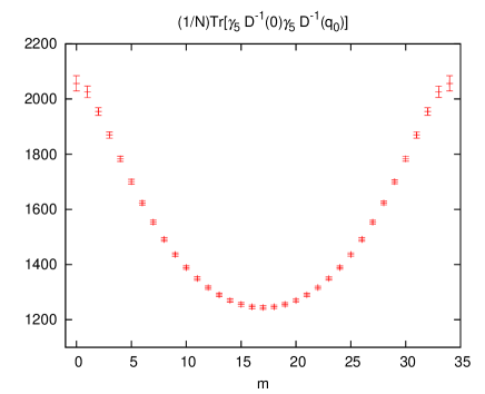
Figure 1: ${1\over N}{\rm Tr}\left[\gamma_{5}D^{-1}(0)\gamma_{5}D^{-1}(q_{0}={2\pi m\over\ell_{0}L})\right]$ as a function of $m$ at $b$=0.36 and $\kappa$=0.155. The error bars of $y$-axis are 100 times enhanced artificially.

Meson correlation functions are extracted from (4). By making the sum over $q_{0}={2\pi m\over\ell_{0}L}$, $0\leq m\leq\ell_{0}L-1$ for $0\leq n_{0}\leq\ell_{0}L-1$, we obtain the correlation function for the quarks living in a $\ell_{0}L\times L^{3}$ finite box.

In fig. 2, we show the pion correlation function $C_{55}(n_{0})$ both for $\ell_{0}=1$ and $2$. For $\ell_{0}$ =1, signals are good for entire range of $0\leq n_{0}\leq L=17$. However, contaminations from higher excited states are so large that we can not reliably extract the information of the lowest state. On the other hand, for $\ell_{0}$ =2, although the data points are quite smooth as a function of $n_{0}$, the error bars become large for larger separation. This is in sharp contrast to the convention calculation of pion correlator, where we know that the error of the pion correrator decreases proportional to the value of the correlator itself. The reason is simple; we extract the correlation function from (4). As is pointed out earler, largest error comes from ${\rm Tr}\left[\gamma_{5}D^{-1}(0)\gamma_{5}D^{-1}(0)\right]$, whose contribution to $C_{AB}(n_{0})$ is independent on $n_{0}$.

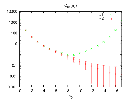
Figure 2: Pion correlation function $C_{55}(n_{0})$ as functions of $n_{0}$ at $b$=0.36 and $\kappa$=0.155. Green symbols represent the results with $\ell_{0}=1$ whereas red symbols are for $\ell_{0}=2$.

We, therefore, expect that constant error contributions are canceled out in effective mass $m_{\rm eff}(n_{0})=\log\left[C(n_{0}-1)/C(n_{0})\right]$ and get good signals even for $\ell_{0}=2$. Results are shown in fig. 3 for both pion (black) and rho meson(red) at $b$=0.36 and $\kappa$=0.155. We clearly see good signals up to $n_{0}\sim 13$, although contributions of higher excitation states are not negligible for small $n_{0}$ due to the use of local meson operators. We then make a three mass fit of the form

$$m_{\rm eff}(n_{0})=\log\left[G(n_{0}-1)/G(n_{0})\right]$$ (12)

$$G(n_{0})={\rm e}^{-m_{1}n_{0}}+a_{2}{\rm e}^{-m_{2}n_{0}}+a_{3}{\rm e}^{-m_{3}n_{0}}$$ (13)

with the fitting range $[3:13]$ for pion and $[2:13]$ for rho meson. The fits are reasonable with $\chi^{2}/$ndf 0.76 for pion and 0.63 for rho meson. We have repeated the above procedure for other $\kappa$ values with $b$=0.36 and 0.37, and these results are used to make discussion in ref.[9].

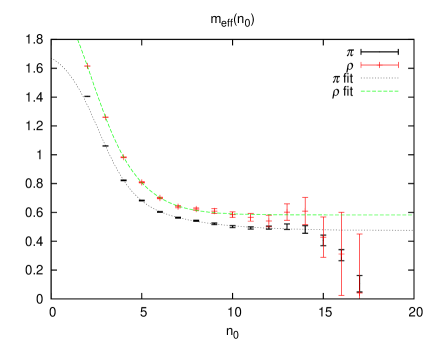
Figure 3: Effective mass $m_{\rm eff}(n_{0})=\log\left[C(n_{0}-1)/C(n_{0})\right]$ as functions of $n_{0}$ for pion (black) and rho meson(red). Fits are made with fitting function (3.1).

4 Smearing

From the above discussion, it is obvious that we have to reduce the effects of higher excitation states to get more reliable results. Usually, this is achieved by constructing spatially extended operators having the same quantum numbers and make a variational analysis. At first sight, it does not seem to be clear how to make spatially extended operators in our one-site model. Nevertheless, it is a rather straightforward generalization of our formulation to construct smeared operators.

Our proposal is summarized as follow. For the meson operator in channel $A$, we replace $\gamma_{A}$ by the following operator having the same quantum number

$$\gamma_{A}\rightarrow D_{s}^{l}\gamma_{A},\ \ \ D_{s}\equiv{1\over 1+6c}\left[1+c\sum_{i=1}^{d-1}\left({\bar{U}_{i}}\Gamma_{i}^{*}+{\bar{U}_{i}^{\dagger}}\Gamma_{i}^{t}\right)\right]$$ (14)

$l$ is the smearing level and ${\bar{U}_{i}}$ is the ape-smeared spatial link variables after making the following transformation several times iteratively

$$U^{\prime}_{i}={\rm Proj_{SU(N)}}\left[(1-f)U_{i}+{f\over 4}\sum_{j\neq i}(U_{j}U_{i}U_{j}^{\dagger}+U_{j}^{\dagger}U_{i}U_{j})\right]$$ (15)

$c$ and $f$ are smearing parameters. (14) is just the one-site version of the smearing adopted in [12]. The smeared meson propagators are given by

$$C_{AB}^{ll^{\prime}}(n_{0})={1\over\ell_{0}N^{3/2}}\sum_{q_{0}}{\rm e}^{-iq_{0}n_{0}}{\rm Tr}\left[D_{s}^{l}\gamma_{A}D^{-1}(0)D_{s}^{l^{\prime}}\gamma_{B}D^{-1}(q_{0})\right],$$ (16)

which can be easily calculated from

$$x_{A}^{l} = Q^{-1}(0)D_{s}^{l}\gamma_{5}\gamma_{A}^{\dagger}z$$ (17)

$$y_{B}^{l^{\prime}}(q_{0}) = D_{s}^{l^{\prime}}y_{B}(q_{0})$$ (18)

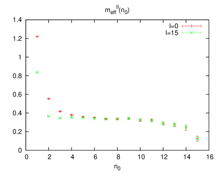
Figure 4: Effective mass $m_{\rm eff}^{ll}(n_{0})=\log\left[C_{55}^{ll}(n_{0}-1)/C_{55}^{ll}(n_{0})\right]$ for pion as functions of $n_{0}$ in $d=2$ TEK model. Red symbols are for unsmeared operator and green symbols are 15 times smeared operator.

To check the validity of the smearing, we have applied it to the $d=2$ TEK model. In two dimension, SU($N$) TEK model is related to the usual lattice theory on a $N\times N$ finite box. Since there is no extra spatial dimension to make ape-smearing, $D_{s}$ takes very simple form

$$D_{s}={1\over 1+2c}\left[1+c\left(U_{1}\Gamma_{1}^{*}+U_{1}^{\dagger}\Gamma_{1}^{t}\right)\right]$$ (19)

Simulations are made with $N$=31, $k$=7, $b$=2.0 and $\kappa$=0.25.

In fig. 4, we show the effective mass of pion both for unsmeared local operator ($l=0$, red symbol) and that of 15 times smeared spatially extended operator ($l=15$, $c=0.4$, green symbol) with $\ell_{0}=1$. The effect of the smearing is significant. We are now making systematic variational analysis for both 2 and 4 dimensional TEK model[13]. We hope to present new results in coming lattice conference.

- [1] A. Gonzalez-Arroyo and M. Okawa, Phys. Lett. B 120 (1983) 174.
- [2] A. Gonzalez-Arroyo and M. Okawa, Phys. Rev. D 27, 2397 (1983).
- [3] A. Gonzalez-Arroyo and M. Okawa, JHEP 07 (2010) 043 [arXiv:1005.1981 [hep-th]].
- [4] A. Gonzalez-Arroyo and M. Okawa, JHEP 12 (2014) 106 [arXiv:1410.6405 [hep-lat]].
- [5] A. Gonzalez-Arroyo and M. Okawa, Phys. Lett. B 718 (2013) 1524 [arXiv:1206.0049 [hep-th]].
- [6] M. Garcia Perez, A. Gonzalez-Arroyo, L. Keegan and M. Okawa, JHEP 01 (2015) 038 [arXiv:1412.0941 [hep-lat]].
- [7] A. Gonzalez-Arroyo and M. Okawa, Phys. Rev. D 88 (2013) 014514 [arXiv:1305.6253 [hep-lat]].
- [8] M. Garcia Perez, A. Gonzalez-Arroyo, L. Keegan and M. Okawa, JHEP 08 (2015) 034 [arXiv:1506.06536 [hep-lat]].
- [9] A. Gonzalez-Arroyo and M. Okawa, [arXiv:1510.05428 [hep-lat]].
- [10] M. Garcia Perez, A. Gonzalez-Arroyo, L. Keegan, M. Okawa and A. Ramos, JHEP 06 (2015) 093 [arXiv:1505.05784 [hep-lat]].
- [11] K. Fabricius and O. Haan, Phys. Lett. B 143 (1984) 459.
- [12] G. Bali, F. Bursa, L. Castagnini, S. Collins, L. Del Debbio, B. Lucini and M. Panero, JHEP 06 (2013) 071.
- [13] M. Garcia Perez, A. Gonzalez-Arroyo and M. Okawa, in preparation.