Validity of the generalized Brink-Axel hypothesis in ²³⁸Np

Abstract

We have analyzed primary $\gamma$-ray spectra of the odd-odd ²³⁸Np nucleus extracted from ²³⁷Np($d,p\gamma$)²³⁸Np coincidence data measured at the Oslo Cyclotron Laboratory. The primary $\gamma$ spectra cover an excitation-energy region of $0\leq E_{i}\leq 5.4$ MeV, and allowed us to perform a detailed study of the $\gamma$-ray strength as function of excitation energy. Hence, we could test the validity of the generalized Brink-Axel hypothesis, which, in its strictest form, claims no excitation-energy dependence on the $\gamma$ strength. In this work, using the available high-quality ²³⁸Np data, we show that the $\gamma$-ray strength function is to a very large extent independent on the initial and final states. Thus, for the first time, the generalized Brink-Axel hypothesis has been experimentally verified for $\gamma$ transitions between states in the quasi-continuum region, not only for specific collective resonances, but also for the full strength below the neutron separation energy. Based on our findings, the necessary criteria for the generalized Brink-Axel hypothesis to be fulfilled are outlined.

Sixty years ago, David M. Brink proposed in his PhD thesis brink that the photoabsorption cross section of the giant electric dipole resonance (GDR) is independent of the detailed structure of the initial state. In his thesis, he expressed his hypothesis as follows: ”If it were possible to perform the photo effect on an excited state, the cross section for absorption of a photon of energy $E$ would still have an energy dependence given by (15)”, where equation (15) refers to a Lorentzian shape of the photoabsorption cross section. Brink’s original idea, the Brink hypothesis, was first intended for the photoabsorption process on the GDR, but has been further generalized, applying the principle of detailed balance, to include absorption and emission of $\gamma$ rays between resonant states axel ; Bartholomew . In addition to assuming independence of excitation energy, there is no explicit dependence of initial and final spins except the obvious dipole selection rules, implying that all levels exhibit the same dipole strength regardless of their initial spin quantum number. We will refer to this as the generalized Brink-Axel (gBA) hypothesis. A review of the history of the hypothesis was given by Brink in Ref. oslo2009 .

The gBA hypothesis has implications for almost any situation where nuclei are brought to an excited state above $\approx 2\Delta$, where $\Delta\approx 1$ MeV is the pair-gap parameter. Here, the nucleus will typically de-excite via $\gamma$-ray emission and/or by emission of particles. In this context, it is usual to translate the $\gamma$-ray cross section $\sigma(E_{\gamma})$ into $\gamma$-ray strength function ($\gamma$SF) by $f(E_{\gamma})=(3\pi^{2}\hbar^{2}c^{2})^{-1}\sigma(E_{\gamma})/E_{\gamma}$.

To describe and model the electric dipole part of the $\gamma$-decay channel, the gBA hypothesis is frequently used, applying in particular the assumption of spin independence RIPL3 . For example, a rather standard approach to calculating $E1$ strength is to apply some variant of the quasi-particle random-phase approximation (QRPA) to obtain $B(E1)$ values as function of excitation energy, and assuming that this $E1$ distribution corresponds to the one in the quasi-continuum; see, e.g., Ref. daoutidis2012 and references therein. Also for $M1$ transitions the gBA hypothesis has been utilized, see e.g. Ref. loens2012 . Furthermore, the hypothesis is also often applied to $\beta$-decay and electron capture for calculating Gamow-Teller and Fermi transition strengths, see e.g. Ref. fantina2012 and references therein. The main reason for its wide range of applications is the drastic simplification of the considered problem, and in some cases it is a key necessity to be able to perform the desired calculation fantina2012 . Hence, the question of whether the hypothesis is valid or not, and under which circumstances, is of utmost importance for multiple reasons: its fundamental impact on nuclear structure and dynamics, and its pivotal role for the description of $\gamma$ and $\beta$ decay for applied nuclear physics, such as input for ($n,\gamma$) cross-section calculations relevant to the $r$-process nucleosynthesis in extreme astrophysical environments arnould2007 and next-generation nuclear power plants IAEA-TECDOC .

However, it is not at all obvious neither from experiment nor theory that the gBA hypothesis is valid. From an experimental point of view, there are two main reasons for this; the hypothesis has primarily been tested at very high excitation energies or with only a few states included. In the first case, compilations show that the width of the GDR varies with temperature and spin, in contradiction to the gBA hypothesis schiller2007 . However, the hypothesis was not originally considered for building the GDR on such highly excited states. Obviously, thermal fluctuations will affect the width of the GDR, but the GDR energy centroid stays rather fixed. Other test cases suffer from large Porter-Thomas (PT) fluctuations PT , since the $\gamma$SF could not be averaged over a sufficient amount of levels 46Ti . In particular, this is the case for lighter nuclei or if levels close to the ground state are considered.

In general, experimental data supporting the gBA hypothesis are rather scarce. For example, $(n,\gamma)$ reactions give $\gamma$SFs consistent with the gBA hypothesis, but in a limited $\gamma$-ray energy range stefanon1977 ; raman1981 ; kahane1984 ; islam1991 ; kopecky1990 . Furthermore, data on the ⁸⁹Y$(p,\gamma)^{90}$Zr reaction point towards deviations from the gBA hypothesis netterdon2015 . There have also been various theoretical attempts to test the gBA hypothesis and modifications or even violations are found misch2014 ; johnson2015 . For some theoretical applications, the assumption of the gBA hypothesis is successfully applied koeling1978 ; horing1992 ; gu2001 ; betak2001 ; hussein2004 . We may learn from these experimental and theoretical attempts that the structure and dynamics of the system represents important constraints.

In this Letter, we address the gBA hypothesis from an experimental point of view, and we provide the needed criteria for the hypothesis to be valid for $\gamma$ decay below the neutron threshold by a detailed analysis of the ²³⁸Np $\gamma$SF. The ²³⁸Np nucleus is probably the ultimate case to test the gBA hypothesis, as it is an odd-odd system with extremely high level density. Already a few hundred keV above the ground state, we find a level density of $\approx 200$ MeV^-1, which increases to $\approx 43\cdot 10^{6}$ MeV^-1 at the neutron separation energy of $S_{n}=5.488$ MeV. In a previous study 238Np , the level density and $\gamma$SF were extracted from the distributions of primary $\gamma$-rays measured in the ²³⁷Np$(d,p\gamma)^{238}$Np reaction. This very rich data set represents ideal conditions for testing the gBA hypothesis where the PT fluctuations are negligible due to the high level density. In the following, we utilize the primary matrix of initial excitation energy $E_{i}$ versus $\gamma$-ray energy 238Np .

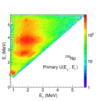
Figure 1: (Color online) Primary $\gamma$-ray matrix of ²³⁸Np 238Np .

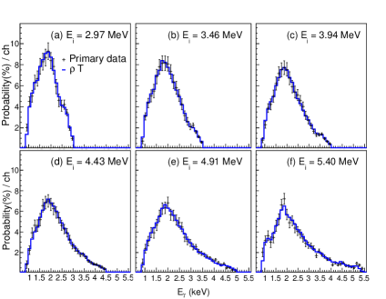
Figure 2: (Color online) Primary $\gamma$-ray spectra (data points) at various initial excitation energies compared to the product $\rho(E_{i}-E_{\gamma}){\cal{T}}(E_{\gamma})$ (blue curve).

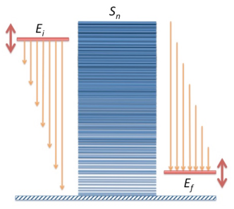
Figure 3: (Color online) The procedure to extract $\gamma$SFs as function of initial $E_{i}$ (left) and final $E_{f}$ (right) excitation energies. The blue-shaded region (middle) illustrates the exponentially increasing level density as function of excitation energy. The two $\gamma$SFs are limited to $E_{\gamma}<E_{i}$ and $E_{\gamma}<S_{n}-E_{f}$, respectively, where $S_{n}$ is the neutron separation energy.

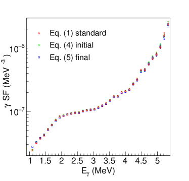
Figure 4: (Color online) Comparison between the three $\gamma$SFs obtained by Eqs. (1), (4) and (5).

Figure 1 shows the primary $U(E_{\gamma},E_{i})$ $\gamma$ spectra (unfolded with the detector response functions) as function of initial excitation energy $E_{i}$. We now normalize $U$ to obtain the probability that the nucleus emits a $\gamma$-ray with energy $E_{\gamma}$ at excitation energy $E_{i}$ by $P(E_{\gamma},E_{i})=U(E_{\gamma},E_{i})/\sum_{E_{\gamma}}U(E_{\gamma},E_{i})$. The probability is assumed to be factorized into:

$$P(E_{\gamma},E_{i})\propto\rho(E_{i}-E_{\gamma}){\cal{T}}(E_{\gamma}).\$$ (1)

According to Fermi’s golden rule dirac ; fermi , the decay probability $P$ is proportional to the level density at the final energy $\rho(E_{i}-E_{\gamma})$. The decay probability is also proportional to the squared transition matrix element $|\langle f|\hat{T}|i\rangle|^{2}$ between initial $|i\rangle$ and final $\langle f|$ states, which is represented by the $\gamma$-ray transmission coefficient ${\cal{T}}$ when averaged over many transitions with the same transition energy $E_{\gamma}$. For now, let us assume that the transmission coefficient depends only on $E_{\gamma}$, in accordance with the gBA hypothesis.

The factorization given in Eq. (1) allows us to simultaneously extract the functions $\rho$ and ${\cal{T}}$ from the two-dimensional probability landscape $P$. The technique used, the Oslo method Schiller00 , requires no models for these functions. In the present case 238Np , we have fitted each vector element of the two functions to the following region of the $P$ matrix: $3.0\leq E_{i}\leq 5.4$ MeV and $E_{\gamma}>0.84$ MeV. The justification of this standard procedure has been experimentally tested for many nuclei by the Oslo group compilation and a survey of possible errors for the Oslo method was presented in Ref. Lars11 .

The applicability of Eq. (1) and the quality of the least $\chi^{2}$ fitting procedure are demonstrated in Fig. 2. The agreement is very satisfactory with a $\chi^{2}_{\rm reduced}=0.81$, and indicates that the determination of the level density $\rho$ and the transmission coefficient ${\cal{T}}$ works well. In the following we assume that $\rho$ and ${\cal{T}}$ are normalized according to the procedure in Ref. Schiller00 . Thus, we introduce a normalization factor $N$ in Eq. (1), which only depends on the initial excitation energy, and rewrite:

$$N(E_{i})P(E_{\gamma},E_{i})=\rho(E_{i}-E_{\gamma}){\cal{T}}(E_{\gamma}),\$$ (2)

which determines the normalization factor by

$$N(E_{i})=\frac{\int_{0}^{E_{i}}{\cal T}(E_{\gamma})\rho(E_{i}-E_{\gamma})\,{\mathrm{d}}E_{\gamma}}{\int_{0}^{E_{i}}\,P(E_{\gamma},E_{i})\,{\mathrm{d}}E_{\gamma}}.$$ (3)

It is an open question if the transmission coefficient ${\cal{T}}$ actually changes with excitation energy, as this procedure gives an average ${\cal{T}}$ for a rather wide range of initial excitation energies in the standard Oslo method. Hence, it is possible that variations of ${\cal{T}}$ as function of initial (or final) excitation energy might be masked. In the following, we will investigate whether ${\cal{T}}$ depends on initial and final excitation energies in order to test the gBA hypothesis. For this we collect $\gamma$ transitions from certain initial states or $\gamma$ transitions into certain final states as illustrated in Fig. 3.

The idea is that, as the level density $\rho$ is known, the $\gamma$ transmission coefficient can be studied in detail per excitation energy bin simply by $NP/\rho$ from Eq. (2).

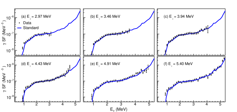
Figure 5: (Color online) The $\gamma$SFs as function of initial excitation energies (data points), see Eq. (4). The blue curve is obtained by the standard Oslo method, see Eq. (1). The excitation energy bins are 121 keV broad.

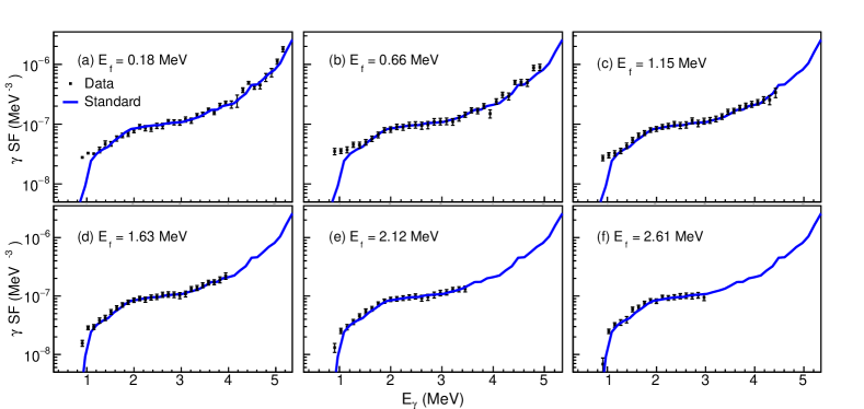
Figure 6: (Color online) The $\gamma$SFs as function of final excitation energies (data points), see Eq. (5). See text of Fig. 5.

More specifically, we get for initial states:

$${\cal T}(E_{\gamma},E_{i})=\frac{N(E_{i})P(E_{\gamma},E_{i})}{\rho(E_{i}-E_{\gamma})},$$ (4)

or alternatively for final states:

$${\cal T}(E_{\gamma},E_{f})=\frac{N(E_{f}+E_{\gamma})P(E_{\gamma},E_{f}+E_{\gamma})}{\rho(E_{f})},$$ (5)

where $E_{f}=E_{i}-E_{\gamma}$. One should note that the normalization factor $N$ is calculated from the assumption that both ${\cal T}(E_{\gamma},E_{i})$ and ${\cal T}(E_{\gamma},E_{f})$ fluctuate on the average around the excitation-independent ${\cal T}(E_{\gamma})$, see Eq. (3).

We now translate the $\gamma$ transmission coefficient into $\gamma$SF by kopecky1990

$$f(E_{\gamma})=\frac{1}{2\pi}\frac{{\cal T}(E_{\gamma})}{E_{\gamma}^{2L+1}},$$ (6)

where we assume that dipole radiation ($L=1$) dominates the $\gamma$ decay in the quasi-continuum. This is motivated by known discrete $\gamma$-ray transitions from neutron capture kopecky1990 and angular distributions of primary $\gamma$-rays measured at high excitation energies larsen2013 .

To check that the normalization function $N(E_{i})$ is reasonable, we compare the three $\gamma$SFs obtained from Eqs. (1), (4) and (5), where $f(E_{\gamma},E_{i})$ and $f(E_{\gamma},E_{f})$ are averaged over initial and final excitation energies by

$$f_{i}(E_{\gamma}) = \frac{1}{S_{n}-E_{\gamma}}\int_{0}^{S_{n}-E_{\gamma}}f(E_{\gamma},E_{i})\,\mathrm{d}E_{i},$$ (7)

$$f_{f}(E_{\gamma}) = \frac{1}{S_{n}-E_{\gamma}}\int_{E_{\gamma}}^{S_{n}}f(E_{\gamma},E_{f})\,\mathrm{d}E_{f},$$ (8)

respectively. Figure 4 demonstrates that the three extraction methods give $f(E_{\gamma})=f_{i}(E_{\gamma})=f_{f}(E_{\gamma})$ within the experimental errors. This supports the normalization function $N$ used in Eqs. (4) and (5).

We are now ready to compare our data with the gBA hypothesis. Figure  5 shows the initial excitation energy dependent $f(E_{\gamma},E_{i})$ compared to $f(E_{\gamma}$) obtained with the standard Oslo method (blue curve). The excitation-energy bins are $\Delta E_{i}=121$ keV wide, and only every fourth gate is shown. The overall agreement is excellent, and the same holds also for all the bins not shown. It is clear that each of these $\gamma$SFs are built on a specific initial excitation-energy gate, but with no specific final state, as illustrated in Fig. 3. However, for a given $E_{\gamma}$ and $E_{i}$, the final excitation energy is determined. Since all data points coincide with $f(E_{\gamma})$, this also indicates independence of the final state.

Any potential dependence of the final state is best analyzed by $f(E_{\gamma},E_{f})$ as given by Eq. (5) and shown in Fig. 6. Again, we find an excellent agreement between the various $\gamma$SFs with $\gamma$ transitions into specific final excitation-energy bins. However, there are discrepancies for $E_{\gamma}<1$ MeV, which feed final states below $\approx 1$ MeV. At these energies, $f(E_{\gamma},E_{f})$ shows an increase compared to the average $f(E_{\gamma})$. These $\gamma$ transitions could possibly be due to vibrational modes built on the ground state, and, if this be true, not part of a general $\gamma$SF extracted in the quasi-continuum with the standard Oslo method. Vibrational levels are strongly populated in inelastic scattering, such as the reactions ^237,239Np($d,d^{\prime}$)^237,239Np performed by Thompson et al. dd . In that work, levels built on vibration modes were seen for excitation energies in the $\approx 0.9$-MeV and $\approx 1.6$-MeV regions. A similar population of vibrational states has been observed in the ²³⁸U(¹⁶O,¹⁶O^′)²³⁸U and ²³⁸U($\alpha$,$\alpha^{\prime}$)²³⁸U reactions aa . By means of $\alpha\gamma$-coincidences, a concentration of $E_{\gamma}\approx 1$ MeV transitions depopulating $\beta$-, $\gamma$- and octupole vibrational bands has been seen. Thus, the enhanced $\gamma$SF found in our data at low excitation energies with $E_{\gamma}\approx 1$ MeV is likely due to deexcitation of vibrational structures, which do not show up in the high level density quasi-continuum.

The excellent agreement between excitation energy dependent and independent $\gamma$SFs indicate that PT fluctuations are small compared to the experimental errors for the system studied. For the $\chi_{\nu}^{2}$ distribution, which governs the PT fluctuations, the relative fluctuations are given by $r=\sqrt{(2/\nu)}$ where $\nu$ is the number of degrees of freedom murray1975 . Typically, we have at 2.0 and 4.0 MeV of excitation energies, $\approx 1200$ and $\approx 120000$ levels within the 121-keV excitation energy bins. Taking the number of levels as the number of degrees of freedom, we obtain $r=4.1$ % and 0.4 %, respectively, which should be compared with the data error bars of Figs. 5 and 6 of typically 10%. Thus, in the ²³⁸Np case, the PT fluctuations are smaller than the statistical errors and not significant. However, for systems with less than $\approx 200$ levels per bin the PT fluctuations will exceed the experimental statistical error of 10%. This gives guidance for the necessary statistics and the required level density for the gBA hypothesis to be fulfilled.

In conclusion, we have studied the $\gamma$-ray strength function between well defined excitation energy bins in ²³⁸Np. For the first time, the generalized Brink-Axel hypothesis has been verified in the nuclear quasi-continuum. The discrepancies seen in the low excitation energy region are probably caused by decay of vibrational states built on the ground state. These excitation modes are not part of the $\gamma$-ray strength function of the quasi-continuum. The validity of the generalized Brink-Axel hypothesis requires that Porter-Thomas fluctuations are low by averaging over a sufficient amount of levels compared to the experimental errors.