Ground-based detectors in very-high-energy gamma-ray astronomy

Abstract

Following the discovery of the cosmic rays by Victor Hess in 1912, more than 70 years and numerous technological developments were needed before an unambiguous detection of the first very-high-energy gamma-ray source in 1989 was made. Since this discovery the field on very-high-energy gamma-ray astronomy experienced a true revolution: A second, then a third generation of instruments were built, observing the atmospheric cascades from the ground, either through the atmospheric Cherenkov light they comprise, or via the direct detection of the charged particles they carry. Present arrays, 100 times more sensitive than the pioneering experiments, have detected a large number of astrophysical sources of various types, thus opening a new window on the non-thermal Universe. New, even more sensitive instruments are currently being built; these will allow us to explore further this fascinating domain. In this article we describe the detection techniques, the history of the field and the prospects for the future of ground-based very-high-energy gamma-ray astronomy.

Résumé: Détecteurs au sol en Astronomie Gamma de Très Haute Energie

Depuis la découverte des rayons cosmiques en 1912 par Victor Hess, il aura fallu près de 70 ans et de nombreux développements, pour aboutir à la première détection d’une source gamma de très haute énergie en 1989. Depuis cette découverte, le domaine de l’astronomie gamma de très haute énergie a vécu une véritable révolution: des détecteurs de deuxième, puis de troisième génération ont vu le jour, observant les cascades atmosphériques depuis le sol, soit à travers l’émission Tcherenkov atmosphérique qui les accompagne, soit en détectant directement les particules chargées qui les composent. Les réseaux récents, environ 100 fois plus sensibles que les plus anciens, ont détecté de très nombreuses sources astrophysiques de types variés et ont ainsi ouvert une nouvelle fenêtre sur l’Univers non thermique. De nouveaux réseaux de télescopes encore plus sensibles, en cours de construction, vont nous permettre de pousser encore plus loin l’exploration de ce domaine fascinant. Dans cet article, nous décrivons les techniques de détection, dressons un panorama historique du domaine et présentons les perspectives pour le futur de l’astronomie gamma de très haute énergie au sol. Keywords : Gamma-rays; Cherenkov Detectors; Imaging Atmospheric Cherenkov Telescopes Mots-clés : Rayons Gammas ; Détecteurs Tcherenkov; Télescopes à effet Cherenkov Atmosphériques

Astrophysics

1 Introduction - Atmospheric Showers

The field of very-high energy (VHE) gamma-ray astronomy has been intimately linked to the physics of cosmic rays (CRs) since the discovery of the latter in 1912. Indeed, it was rapidly noticed that processes giving rise to non-thermal, very-high-energy particles would also lead, via the interaction of those particles with the interstellar medium (matter and radiation), to the production of very high energy photons [1].

Although the first attempts to detect the Cherenkov light from the charged particles traveling in the atmosphere dates back from 1953 [2], after a suggestion from Blackett [3], it took several decades before the emergence of ground-based very-high-energy gamma-ray astronomy. Before even trying to distinguish the gamma rays from the charged cosmic rays, the main challenges to overcome at that time were to actually detect a Cherenkov signal itself. The difficulties in the detection were caused by the very short duration of the flashes, the small intensity of the signal and the very large background from the night sky (light from stars and scattered light, that required the use of sensitive detectors and fast electronics.

In 1989, the first source of VHE gamma rays was discovered by the Whipple collaboration [4]. This seminal detection opened a new window in gamma-ray astronomy and started a very productive research field in an energy domain which is essentially accessible only to ground-based instruments.

In this paper, we discuss various concepts of detecting gamma rays from the Earth’s surface as well as major ground-based experiments of the past, present and near future that largely shaped and continue to shape the booming field of gamma-ray astronomy.

1.1 Development of atmospheric Showers

Ever since 1912, when Victor Hess announced the first evidence that ionizing radiation constantly impinges on the Earth’s atmosphere, scientists are continuing to develop efficient techniques to detect and study this radiation.

When a high-energy particle ($\gamma$ ray or charged nucleus) enters the atmosphere, it can interact with the atmospheric nuclei through various processes, leading to the development of a so-called “extended air shower (EAS)” of particles. Electromagnetic showers, initiated by high energy photons or electrons, are governed by mainly two elementary processes:

• Production of pairs of $e^{\pm}$ by the conversion of high energy photons in the Coulomb field of the nuclei,

• Bremsstrahlung emission of $e^{\pm}$ in the same Coulomb field, leading the production of further high energy photons.

The energy of the impinging particle is then redistributed over many particles as the shower develops in the atmosphere. Pair production and bremsstrahlung emission have the same characteristic length, the “electromagnetic radiation length”, defined for a material of mass and atomic numbers $A$ and $Z$ as:

$$X_{0}=\left[{4\alpha r_{e}^{2}\frac{N_{A}}{A}Z^{2}\ln\left(183\,Z^{-1/3}\right)}\right]^{-1}\;\left[\mathrm{\ g}\mathrm{\ cm^{-2}}\right]$$ (1)

where $\alpha=1/137$ is the fine structure constant, $r_{e}$ the classical electron radius and $N_{A}$ the Avogadro number. This quantity, expressed as a density-integrated thickness $X=\int\!\!\rho\,\mathrm{d}z$, represents roughly the amount of traversed matter after which an electron loses a significant fraction of its energy by bremsstrahlung. The bremsstrahlung emission leads to an average energy loss as a function of thickness $X$:

$$E(X)=E_{0}\exp\left(-\frac{X}{X_{0}}(1+b)\right)$$ (2)

where $\displaystyle b=1/\left(18\ \ln(183/Z^{1/3})\right)=0,0122$ in air, so that, on average, each electron looses half of its energy after a depth $R=X_{0}\ln 2$ . Similarly, the integrated pair-creation probability is given by:

$$\mu(X)=1-\exp\left(-\frac{X}{X_{0}}\left(\frac{7}{9}-\frac{b}{3}\right)\right)$$ (3)

In the atmosphere (dry air), the radiation length corresponds to $36.7\mathrm{\ g}\mathrm{\ cm^{-2}}$. The atmosphere is therefore a thick calorimeter of $\sim 27$ radiation lengths compared to about $\sim 10X_{0}$ for gamma-ray satellites and $\sim 25X_{0}$ for particle physics calorimeter such as those of ATLAS or CMS at the CERN Large Hadron Collider.

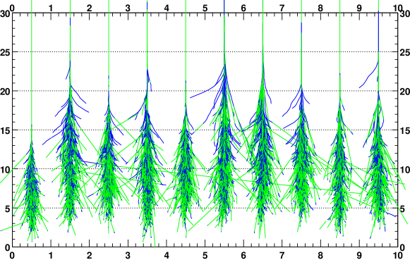
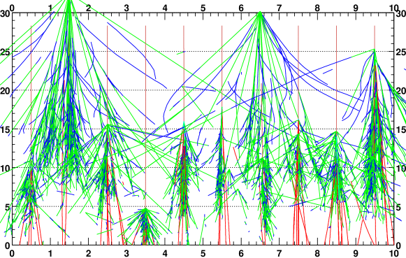
Figure 1: Illustration of the intrinsic variability of shower development. Top: Simulation of 10 showers, each initiated by a $\gamma$ ray of $300\mathrm{\ GeV}$. Bottom: Simulation of 10 showers initiated by a proton of the same energy. Due to larger transverse momentum transfers, hadronic showers show larger fluctuations. From [5].

It has to be noted that, due to its varying density, the atmosphere is a strongly inhomogeneous calorimeter. At sea level, for an atmospheric density of $\sim 1.2\mathrm{\ kg}\mathrm{\ m^{-3}}$, one radiation length corresponds to $\sim 300\mathrm{\ m}$. At $10\mathrm{\ km}$ altitude (roughly the altitude of the maximum of development of the showers), the radiation length corresponds to a 3 times larger distance ($\sim 1\mathrm{\ km}$). This has an important consequence: as a shower penetrates deeper in the atmosphere, its development accelerates due to the larger amount of target matter. In a homogeneous calorimeter, the depth of the shower maximum depends logarithmically on the energy of the primary particle. In the atmosphere, the evolution of the altitude of the shower maximum is even slower. This can easily be shown in the framework of the simplified model of an isothermal atmosphere in hydrostatic equilibrium. Then, one finds:

$$z_{\mathrm{max}}=z_{0}\log\frac{\rho_{0}z_{0}}{X_{0}}-z_{0}\log\left(\log\left(\frac{E_{0}}{E_{c}}\right)\right)\approx 9\mathrm{\ km}-8.4\mathrm{\ km}\times\log\left(\log\left(\frac{E_{0}}{1\mathrm{\ TeV}}\right)\right)$$ (4)

where $z_{0}=RT/gM\approx 8.4\mathrm{\ km}$, $T$ being the absolute temperature, $R$ the perfect gas constant, $M$ the equivalent molar mass for air and $g$ the gravity acceleration. The conclusion remains valid in a more realistic model of the atmosphere.

Additional processes play a significant role in the shower development, mainly at low energy:

• Multiple scattering of charged particles, leading to shower broadening;

• Energy losses of $e^{\pm}$ by ionization and atomic excitation, leading to rapid extinction of the shower when the energy of the charged particles in the shower pass below the so-called “critical energy” ($E_{c}=83\mathrm{\ MeV}$ in the air);

• Electron scattering and positron annihilation which leads to an excess of $\sim 10\%$ of electrons compared to positrons (“charge excess”), which in turn can produce a significant radio emission signal (“Askaryan effect”).

• The Earth’s magnetic field which broadens the shower in the East-West direction.

At high energy, photo-production or electro-production of hadrons can occasionally give rise to a hadronic component in electromagnetic showers. However the corresponding cross-sections are typically a factor or $10^{-3}$ smaller than that of pair creation.

Hadronic showers are more complicated to describe, and depend on several different characteristic lengths (nuclear interaction length, decay lengths for unstable particles, radiation length) so no universal scaling is applicable. They comprise several components:

• Hadronic components: nuclear fragments resulting from collision with atmospheric nuclei, isolated nucleons, $\pi$ and $K$ mesons, etc.,

• Electromagnetic component resulting in particular from the decay of neutral pions into $\gamma$ rays,

• High energy muons resulting from the decay of charged mesons ($\pi^{\pm}$ and $K^{\pm}$ mainly),

• Atmospheric neutrinos resulting from the decay of mesons and muons ($\pi^{\pm}$, $K^{\pm}$ and $\mu^{\pm}$).

The electromagnetic and hadronic showers are illustrated in Fig. 1. Hadronic showers are more irregular, often comprising several electromagnetic sub-showers.

1.2 Semi-analytic model of electromagnetic showers

In the 1950’s, Greisen [6] proposed a semi-empirical model of the electromagnetic shower development that, in particular, takes into account ionization losses which where neglected in the previous models.

This models introduces a shower age parameter, which depends on the primary energy $E_{0}$, the critical energy $E_{c}$ and the reduced depth $t=X/X_{0}$:

$$s=\frac{3t}{t+2y}\hbox{ with }y=\ln\left(\frac{E_{0}}{E_{c}}\right)$$ (5)

The age is $s=0$ at the start of the shower, $s=1$ at the depth of shower maximum $t_{\mathit{max}}=y=\ln(E_{0}/E_{c})$ and $s>1$ in the following extinction phase. The semi-empirical Greisen formula gives the average number of electrons at depth $t$ and at the depth of shower maximum $t_{\mathit{max}}$ respectively:

$$\overline{{N_{e}}}(t)=\frac{0,31}{\sqrt{y}}\exp\left[t\left(1-\frac{3}{2}\ln s\right)\right]\leavevmode\nobreak\ \leavevmode\nobreak\ \longrightarrow\leavevmode\nobreak\ \leavevmode\nobreak\ \overline{{N_{e}}}(t_{\mathit{max}})=\frac{0,31}{\sqrt{y}}\left(\frac{E_{0}}{E_{c}}\right)$$ (6)

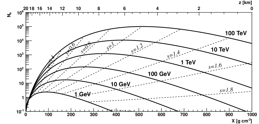
Figure 2: Illustration of the development of electromagnetic showers in an hydrostatic, isothermal atmosphere, following the Greisen semi-empirical model. The solid lines indicate the number of electrons and positrons in the shower as function of depth. The dashed lines corresponds to equal-age curves.

Orders of magnitude for the number of particles and the altitude of the maximum development of showers are given in Table 1 and shown in Fig. 2.

$E_{0}$	$T_{\mathit{max}}(\mathrm{\ g}\mathrm{\ cm^{-2}})$	Altitude (m)	$N_{e}(t_{\mathit{max}})$
$30\mathrm{\ GeV}$	$216$	$12000$	$50$
$1\mathrm{\ TeV}$	$345$	$8000$	$1200$
$1000\mathrm{\ TeV}$	$600$	$4400$	$0,9\times 10^{6}$
$10^{19}\mathrm{\ eV}$	$936$	$1200$	$7,4\times 10^{9}$

Table 1: Orders of magnitude of shower development for different primary energies

1.3 Cherenkov Radiation

Ultra-relativistic particles in the shower travel faster than the speed of light in the air. Coherent depolarization of the dielectric medium (of refractive index $n$) results in a forward-beamed emission called “Cherenkov Radiation”, emitted along a cone with opening angle $\theta_{c}$, and with a number of photons emitted per unit track length $\mathrm{d}z$ of charged particle and per unit wavelength $\mathrm{d}^{2}N/\mathrm{d}z\mathrm{d}\lambda$ (See Fig 3):

$$\cos\theta_{c}=\frac{1}{\beta n},\leavevmode\nobreak\ \leavevmode\nobreak\ \leavevmode\nobreak\ \leavevmode\nobreak\ \leavevmode\nobreak\ \frac{\mathrm{d}^{2}N_{ph}}{\mathrm{d}x\mathrm{d}\lambda}=2\pi\alpha Z^{2}\frac{\sin^{2}\theta_{c}}{\lambda^{2}}$$ (7)

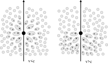
Figure 3: Left: Illustration of the polarization of the medium induced by the crossing of a relativistic particle. Right: Construction of Cherenkov wave-front.

In general, the refractive index depends on the density of air (and therefore on the altitude), so the Cherenkov yield does as well. The refractive index of air is mainly a function of the pressure (or density):

$$(n-1)=2.92\times 10^{-4}\times\frac{P}{P_{0}}\times\frac{288.15\mathrm{\ K}}{T}$$ (8)

In the simplified case of an hydrostatic, isothermal atmosphere, the density as function of altitude reads $\rho(z)=\rho_{0}\exp(-z/z_{0})$, with $z_{0}=RT/gM=8.4\mathrm{\ km}$ and $\rho_{0}=1.2\mathrm{\ kg}\mathrm{\ m^{-3}}$. Under the approximation of small angles, $\sin^{2}\theta\approx 2(n-1)$ and for essentially vertical charged particles, the Cherenkov yield per unit thickness $\mathrm{d}X=X/z_{0}\times\mathrm{d}z$, can be then expressed analytically:

$$\frac{\mathrm{d}^{2}N_{ph}}{\mathrm{d}X\,\mathrm{d}\lambda}=2\pi\alpha Z^{2}\frac{\sin^{2}\theta_{c}}{\lambda^{2}}\times\frac{z_{0}}{X}\approx\frac{4\pi\alpha Z^{2}}{\rho_{0}\lambda^{2}}\times 2.92\times 10^{-4}\times\frac{288.15\mathrm{\ K}}{T}$$ (9)

Remarkably, this quantity does not depend on the altitude: the Cherenkov yield, when expressed in the natural variable describing the shower development, does not depend on the local density. Under these approximations, the total amount of Cherenkov light emitted by a shower is given by an integral over the shower age:

$$\frac{\mathrm{d}N_{ph}}{\mathrm{d}\lambda}=\int\mathrm{d}XN_{e}(t)\times\frac{\mathrm{d}^{2}N_{ph}}{\mathrm{d}X\,\mathrm{d}\lambda}=6\times 0.31\sqrt{y}X_{0}\times\frac{E_{0}}{E_{c}}\times\frac{\mathrm{d}^{2}N_{ph}}{\mathrm{d}X\,\mathrm{d}\lambda}\int\frac{\mathrm{d}s}{(3-s)^{2}}\exp\left(\frac{2s}{3-s}\left(1-\frac{3}{2}\ln s\right)\right)$$ (10)

To a correction factor $\sqrt{y}$ that varies only between 2.2 and 3.4 for $E_{0}$ between $10\mathrm{\ GeV}$ and $10\mathrm{\ TeV}$, the total amount of Cherenkov light is therefore almost proportional to the primary energy, thus making a calorimetric measurement possible even in an strongly inhomogeneous environment. This is further confirmed by more elaborated, realistic simulations.

1.4 Angular distribution and light pool

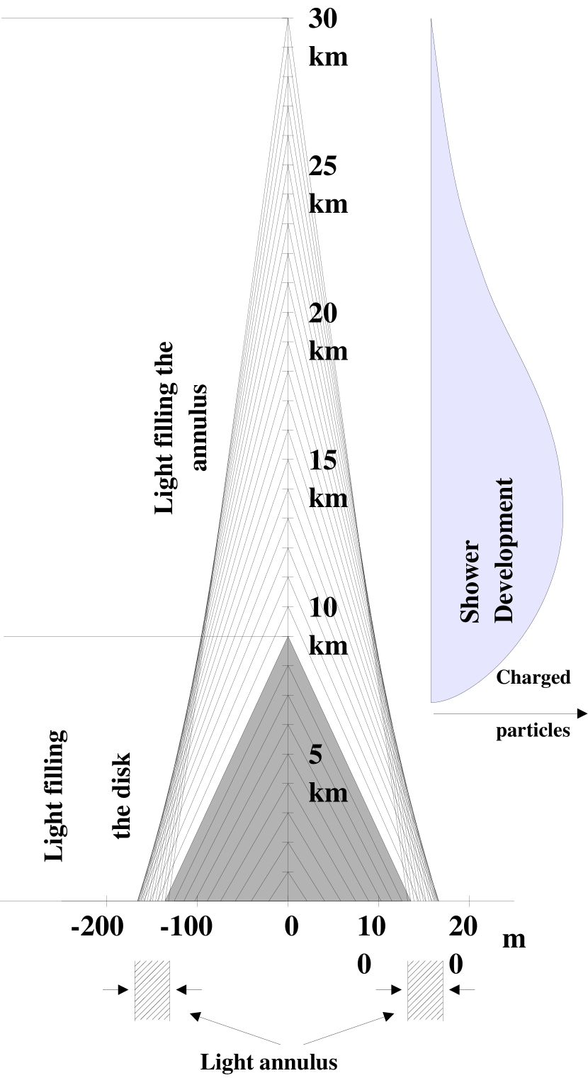
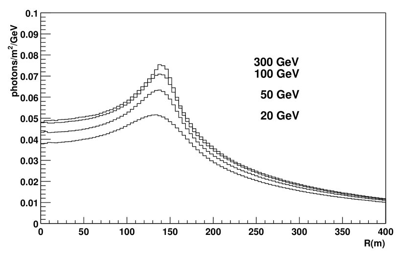
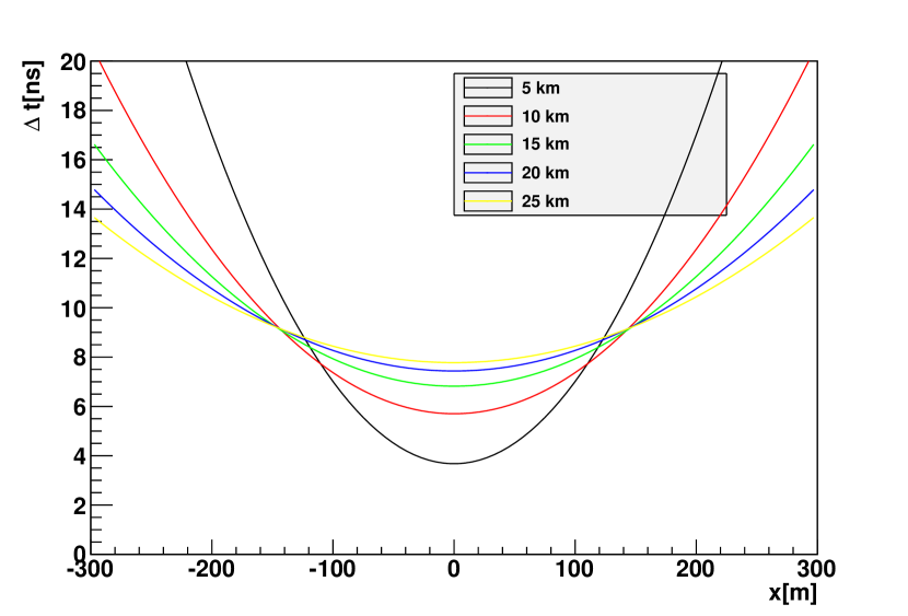
Figure 4: Left: Shower development. Top Right: Lateral profile of showers of different energies at sea level. Bottom Right: Time delay as function of lateral distance for various altitudes of emission.

Due to the evolution of the atmospheric density with altitude, the Cherenkov angle increases from $\sim 0.2^{\circ}$ at an altitude of $\sim 30\mathrm{\ km}$ to $\sim 1.5^{\circ}$ at sea level. The effect of this variation is illustrated for vertical showers in Fig. 4, left, and is responsible for the formation of a light annulus at a distance of $\sim 150\mathrm{\ m}$ from the shower impact on the ground: the variation of the Cherenkov angle with altitude almost exactly compensates the effect of the varying distance to the ground.

Similarly, the spread of the arrival time of the photons on the ground results from two different effects, somewhat in competition: The charged particle in the shower travels faster than light. Therefore, close to the shower axis, the photons emitted at low altitude reach the detector before those emitted at high altitude. At large impact distance however, the photons emitted at low altitude have a longer geometrical trajectory (track of the charged particle to the emission point + track of the photon itself) than those emitted at high altitude, and reach the detector after the latter. At a distance of $\sim 120\mathrm{\ m}$ from the shower (Fig. 4, bottom right), the two effects compensate almost exactly, resulting in a very short duration of the shower of $\sim 2\mathrm{\ ns}$. The shower duration can reach $\sim 5\mathrm{\ ns}$ on axis, and increases significantly for impact distances $>200\mathrm{\ m}$. The time integration window of the detectors therefore has a direct impact on their effective area (through their capability to detect distant showers) but also on the amount of integrated night sky background light and therefore on their energy threshold.

1.5 Detection Techniques

VHE gamma-ray astronomy rests on two basic detector technologies:

• Detectors that measure particles of the shower tail reaching the ground. This method provides a snapshot of the shower at the moment it reaches the ground and constitutes the so-called “particle sampler” technique. Those detectors have a very large duty cycle (potentially $100\%$), but rather high energy threshold (as high energy showers are more penetrating and produce charged particles at lower altitude than lower energy showers). Moreover, as they only have access to shower tails, they usually have a rather poor capability to discriminate the showers induced by $\gamma$ rays from the much more numerous showers induced by protons and charged nuclei. Such detectors are usually installed at high altitude to collect more charged particles. Several types of particle samplers have been tried, including scintillator arrays [7], resistive plate chamber carpets [8] and water Cherenkov ponds [9, 10, 11]. A sketch of the Milagro water Cherenkov detector is shown in Fig. 5.

  

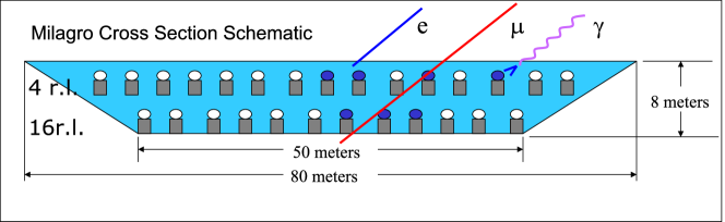
  Figure 5: Sketch of the central Milagro water pond detector.

  In the sampling technique, the direction reconstruction is based on the timing information (simple trigonometric direction measurement using the time of arrival of the signal in each detector), completed by the spatial distribution of the signal on the ground (mainly being used to determine the impact of the shower on the ground).

• Cherenkov detectors for observing showers that died before reaching the ground, through the detection of the Cherenkov light produced in the atmosphere. This method uses the atmosphere as a calorimeter as described in the previous section. Several techniques have been tried in the past. The most successful has been to use optical telescopes to take a “picture” of the showers (recording the Cherenkov light emitted by them), as illustrated in Fig. 6. These so-called “imaging atmospheric Cherenkov telescopes” (IACTs) are characterized by a relatively small field of view (a few degrees angular diameter), low duty cycle ($\sim 10\%$, corresponding to moonless, clear nights), but a very large effective area, corresponding to the size of the light-pool illuminated by the showers ($\sim 10^{5}\mathrm{\ m^{2}}$), and very powerful discrimination capabilities. The experimental challenges are, on the one hand, the very low intensity and short duration of the signal, requiring very fast and sensitive acquisition systems, and, on the other hand, the huge background, from both the night sky luminosity and from the air showers produced by charged cosmic rays. The optimal altitude ($\sim 1500\mathrm{\ m}$) for this technique results from a trade-off between the transparency of the atmosphere to Cherenkov light (pushing for higher altitude) and the development of the shower (leading to larger effective areas, better shower containement and improved calorimetric capabilities at low altitude).

  

  

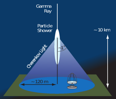
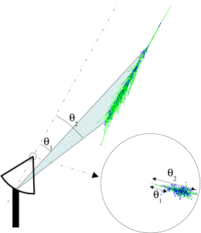
  Figure 6: Imaging Atmospheric Cherenkov technique. Left: the Cherenkov light emitted by the charged particles in the shower is collected by several dishes. Right: The shower angular image is projected into the camera focal plane.

2 The pioneering era

2.1 Early days

After the discovery of cosmic rays by V. Hess, many experiments were designed to study their nature and origin with improved detection techniques. In the 1920s it was a popular belief that all cosmic rays originated from gamma rays. The debate between Robert Millikan (arguing that electrons reaching the earth were produced by Compton scattering of high energy gamma-rays) and Arthur Compton (claiming that cosmic rays were genuine charged particles) made the cover page of the New York Times in 1932. It took 27 years after Hess’ first discovery of CRs until Pierre Auger discovered extended air showers initiated by CRs hitting the atmosphere [12]. The understanding of the shower process grew with time and cosmic ray physicists built balloons to study low energy charged CRs and air shower arrays to detect the high energy tail of the CR spectrum. Meanwhile it was becoming clear that gamma rays are only a tiny fraction of the ionizing radiation hitting the atmosphere. In the early 1980s it was mostly thought that about $1\%$ of the CRs were gamma rays. Nowadays this question is still not completely solved and much smaller flux ratios are assumed. One currently estimates that at most $10^{-4}$ of all particles coming from the Galactic plane are gamma rays, and that an even smaller fraction ($\sim 10^{-5}$) of particles from outside the galactic plane are gamma rays. The expectation in the early days of high gamma-rays fluxes led to strong enthusiasm about abilities to detect sources of gamma rays, but with time these expectations vanished as no unambiguous detection of gamma-ray signals was successful.

It took 19 years to detect Cherenkov light from air showers after the discovery of the effect [13]. In 1953, W. Galbraith and J. V. Jelley built a simple detector and proved that air showers do actually generate Cherenkov light, which could be detected as a fast light flash during clear dark nights [14]. With a threshold of around four times the night sky-noise level, they observed signals with a rate of about one event every two to three minutes. The early detectors consisted of a very simple arrangement, mainly a search-light mirror viewed by a single photomultiplier tube (PMT) as light detector. The first setup was installed in a garbage can for shielding from stray light. In the following years, the technique was refined by using larger mirrors, replacing the single PMT by a few ones arranged in the focal plane and even by trying to detect coincidences between several such simple telescopes .

The three decades from 1960 to the end of the 1980’s saw steady but rather slow progress towards discovering sources of VHE gamma rays. Experiments provided doubtful and often inconsistent results and the funding agencies were not willing to fund large installations, which led many physicists to leave the field.

In 1977 T.C. Weekes, in collaboration with K.E. Turver, presented for the first time concepts for the separation of gamma-ray initiated showers from hadronic background showers [15]. In this work, where computer simulations were used for the first time, the advantages of stereoscopic observation was already advocated.

The “imaging technique”, first proposed by A.M. Hillas in 1985 [16] and developed during these days, consisted of placing a fast camera (initially of 37 PMT’s) at the focal plane of a telescope (Fig. 6) in order to record the image of the shower with an angular resolution better than its size. This technique quickly looked the most promising, which encouraged a few dedicated enthusiasts to stay and pursue developing the instrumentation and the data analysis techniques. Finally, in 1989 a first gamma-ray source, the Crab Nebula, was unambiguously detected with more than 9 standard deviations by the Whipple telescope under the lead of Trevor Weekes [4]. It was the culmination of a long journey for the group that had started in 1968 with a large $10\mathrm{\ m}$ telescope that was completed at the Fred Lawrence Whipple Observatory on Mount Hopkins in Arizona, USA [17].

Three major factors led to the detection of the first gamma-ray source [18]:

• The Whipple collaboration focused on a source that turned out to be the strongest steady state gamma-ray emitter: the Crab Nebula.

• They used a large light collection area telescope ($10\mathrm{\ m}$ diameter) and an imaging camera with 37 PMTs covering a field of view of 3.5 degrees. This allowed recording of true images of air showers, which could be used for an efficient gamma/hadron separation which was not possible with telescopes without imaging cameras.

• The team invested a lot of effort to improve the analysis and gamma/hadron discrimination methods. The analysis developed by the Whipple collaboration in the mid-eighties was based on the combination of a measurement of the shower image orientation [19] and on differences in image shapes between gamma-ray- and hadron-induced showers [20]. The originally rather simple analysis, based on image first and second moments commonly known as Hillas parameters [16], became the basic concept for gamma/hadron separation in the following Cherenkov telescope experiments.

2.2 In all directions …

Subsequent (and mostly contemporaneous with Whipple) experiments confirmed the gamma-ray signal from the Crab Nebula: Crimean GT48 Observatory [21, 22], Yerevan [23], Ala-Too [24], Cangaroo-I [25], The HEGRA array [26], Granite (Whipple+$11\mathrm{\ -m}$ Tel.) [27], MarK V [28], ASGAT [29], Themistocle [30], Telescope Array prototype (TA coll.) [31] and CAT [32]. In 1992, the Whipple collaboration made another great discovery: a signal from an active galactic nuclei (the blazar Markarian 421, located at a red-shift of $z=0.031$) was detected on a level of $30\%$ of the the signal from the Crab Nebula [33]. This opened the window of extragalactic gamma-ray searches.

In 1992, Patrick Fleury and Giuseppe Vacanti invited the community to a conference at Palaiseau with the aim of forming a project of a major imaging Cherenkov telescope [34]. Despite a large participation at the conference and a strong excitement of the community about the new discoveries it was not possible to converge on a joint large scale project. Instead, individual groups pursued developments of the Cherenkov technique in different directions.

Major ideas and experiments followed in the 1990s, exploring different instrumental paths in parallel.

2.2.1 Developments in Imaging Atmospheric Cherenkov Telescopes

• The Cherenkov Array at Thémis (CAT) collaboration built a single dish Cherenkov telescope with $4.7\mathrm{\ m}$ diameter [32]. The novelty of the telescope was a fine grained camera consisting of 546 pixels with an angular size of $0.12^{\circ}$ each. The use of such a camera allowed an accurate analysis of the longitudinal and lateral light profile of the shower image, as discussed in [35], giving a good separation of gamma-ray showers from hadronic ones by means of a goodness of the fit variable and of the pointing angle $\alpha$.

• The HEGRA array in the Canaries island, consisting of 5 IACTs each having $3.3\mathrm{\ m}$ diameter mirror reflector and a camera of 271 pixels, made of PMTs, demonstrated the power of stereoscopic observations. The telescopes were arranged on a square of $100\mathrm{\ m}$ side length with an additional telescope centered in the square. HEGRA did not actually pioneer stereoscopic observations based on a telescope coincidence trigger – this was already done by the Crimean observatory [36] – but it was the first one to find the right separation between the telescopes thanks to Monte-Carlo simulations. Multiple shower images provided information for the optimum discrimination between the Cherenkov light flashes of gamma-ray and cosmic-ray induced showers. Based on the stereo views, an unambiguous reconstruction of the air showers in space became possible, leading to a very significantly improved angular reconstruction of primary particles on an event-by-event basis as well as a much stronger rejection of cosmic-ray induced showers.

• The CANGAROO collaboration constructed a Whipple-like telescope in Australia.

• A group from Durham University upgraded their Mark-VI telescope in Narrabri, Australia combining an idea of a 3-fold coincidence between signals from reflector dishes placed next to each other (the idea originally developed and implemented with smaller reflectors by the Crimean observatory in the 1960s [36]) and an imaging camera in the focus of each dish [28]. The Mark-VI telescope was successfully operated between 1995 and 2000.

2.2.2 Wave-front sampling technique

• The ASGAT [29] and Themistocle [30] arrays, installed in 1988 on the site of a former solar power plant, ”Themis”, in the french Pyrenees, were using a completely independent technique based on fast-timing wave front sampling. ASGAT used 7 parabolic dishes of $7\mathrm{\ m}$ diameter arranged on an hexagonal shape, whereas Themistocle was based on 18 much smaller mirrors ($80\mathrm{\ cm}$ diameter) but spread on a larger area ($170\mathrm{\ m}\times 300\mathrm{\ m}$). Both experiments proved that timing information was useful for reconstructing the shower parameters and for distinguishing gamma rays from charged cosmic rays, quickly confirmed the detection of the Crab Nebula and extended the measurement of its energy spectrum well above $1\mathrm{\ TeV}$.

• Following this first success in the wave-front sampling technique, several groups tried to convert solar farms into gamma-ray detectors during night time. These solar farms were based on the concept of fields of heliostats reflecting the light of the sun onto a furnace at the top of a $\sim 100\mathrm{\ m}$ tower. The use of many large-area heliostats collecting Cherenkov light and focusing it onto a single detector mounted on a tower had advantages to save costs and achieve a low energy threshold. Four installations were in operation: CELESTE in the French Pyrenees [37], STACEE detector using a prototype solar power station near Albuquerque, New Mexico [38], the Keck Solar Two in Barstow, California [39], and the GRAAL detector using the heliostats of the Plataforma Solar in Almería, Spain [40]. Although the approached proved to be very successful in terms of reduction of the energy threshold, the very narrow field of view of these instruments ($\sim 0.5^{\circ}$, corresponding to the angular size of the sun) resulted in a very challenging background subtraction and event identification: the detectors were actually only observing a fraction of the hadronic showers, making them resemble electromagnetic ones. All detectors based on solar heliostat plants were able to detect the strongest sources like the Crab nebula and the flaring Mkn 421 and Mkn 501 but did not reach the sensitivity of the third-generation imaging telescopes and therefore the method was abandoned around 2005 [18].

2.2.3 Particle samplers

• After a first successful prototype Water Cherenkov detector (MILAGRITO [41]), the Milagro [9] experiment operated between 1999 and 2008 in a former water reservoir in the Jemez mountains near Los Alamos, New Mexico, at an altitude of $2630\mathrm{\ m}$. Milagro (see Fig. 5) was composed of a central $60\mathrm{\ m}\times 80\mathrm{\ m}$ pond completed by a sparse $200\mathrm{\ m}\times 200\mathrm{\ m}$ array of 175 “outrigger” water tanks surrounding it. The pond was instrumented with 723 photo-multiplier tubes arranged in two layers the top one being dedicated to the measurement of the electromagnetic component in showers, and the bottom one, located $6\mathrm{\ m}$ below the surface, dedicated to the identification of hadronic showers through their muonic content. Milagro’s large field of view ($2\mathrm{\ sr}$) and high duty cycle ($>90\%$) allowed it to monitor the entire overhead sky continuously, making it well suited to measuring diffuse emission. This is illustrated by the view of the Galactic Plane by Milagro (Fig. 7) above $\sim 20\mathrm{\ TeV}$ , representing 2358 days of data collected by Milagro between July 2000 and January 2007.

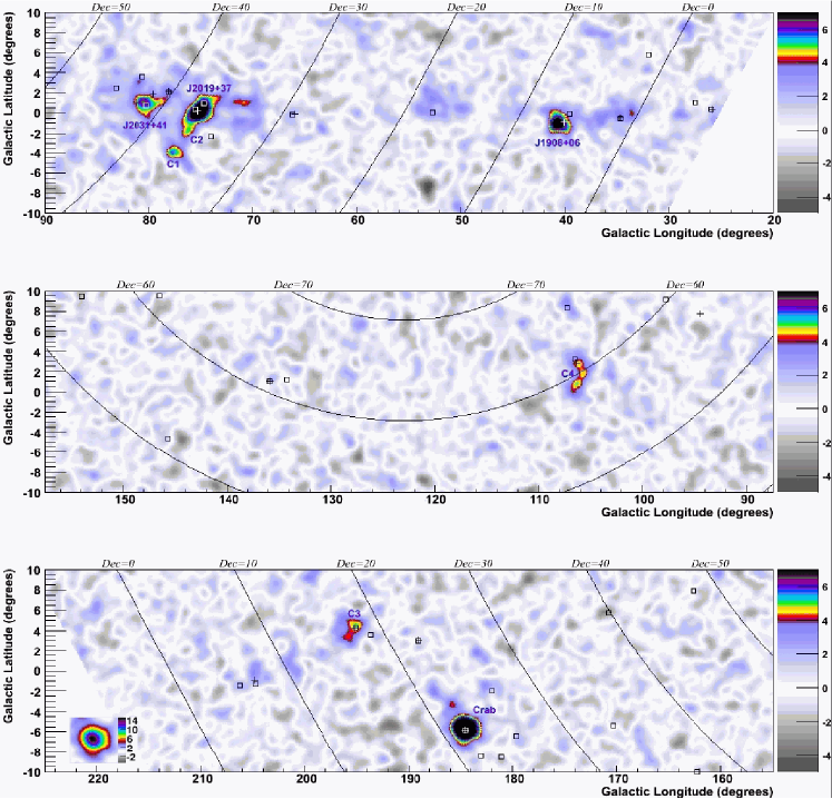
Figure 7: Significance map of the galactic emission as seen by the Milagro Water Cherenkov experiment. The color code shows the pretrial significance, smoothed according to the instrument PSF. From [42].

At the end of this era of so-called second generation of Cherenkov telescopes (around the year 2000) 7 gamma-ray emitters were established: The Crab pulsar wind nebula and the supernova remnant RX J1713.7-3946 as Galactic emitters [43] and Mrk 421, Mrk 501, 1ES 1959+650, PKS 2155-304, and 1ES 1426+428 as extragalactic sources [44], with 1ES 1426+428 being the most distant one (redshift $z=0.129$).

2.3 Digging in the data

The advent of more powerful computers allowed the development of the showers to be simulated to a much better precision, and opened the way to more efficient and elaborated analysis techniques, able to take full advantage of the fine-grained camera with improved acquisition speed.

From the beginning of ground-based gamma-ray astronomy, data analysis techniques have been mostly based on the “Hillas parametrization” [16] of shower images, relying on the fact that gamma-ray images in the focal plane are, to a good approximation, elliptical in shape and intrinsically narrower than hadronic images. In 1985, based on pioneering Monte Carlo simulations, A.M. Hillas proposed to reduce the recorded images to a few parameters, constructed from the first and second moments of the light distribution in the camera, and corresponding to the modeling of the image by a two-dimensional ellipse.

Figure 8: Geometrical definition of the Hillas Parameters. From [45].

These parameters, shown in Fig. 8, are the following:

• image center of gravity (first moments)

• length $L$ and width $w$ of the ellipse (second moments)

• size (total charge of photo-electrons in the image)

• nominal distance $d$ (angular distance between the centre of the camera and the image centre of gravity)

• azimuthal angle of the image main axis $\phi$ (second moments)

• orientation angle $\alpha$ (see Fig. 8.)

The stereoscopic imaging technique, already advocated in 1977 [15] and successfully developed by HEGRA [46] in 1997, allowed a simple, geometrical reconstruction of the shower direction and impact parameter and resulted in a major step in angular resolution as well as in background rejection. The source direction is given by the intersection of the major axes of the shower images in the camera (Fig. 9), and the shower impact point is obtained in a similar manner, using a geometrical intersection of the planes containing the telescopes and the shower axes. The energy is then estimated from a weighted average of each single telescope energy reconstruction. The separation between the showers induced by gamma rays and those induced by charged cosmic rays originates mainly from the larger width of the later.

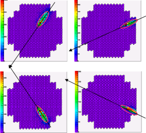
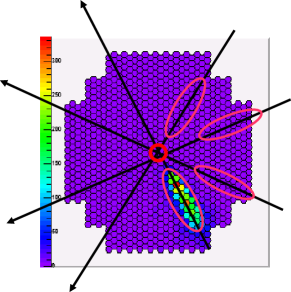
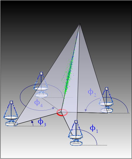
Figure 9: Geometric reconstruction of shower direction and impact in stereoscopic mode. Left: In the camera frame, the main axis of the shower corresponds to a plane that contains the actual shower track and the telescope. The primary particle direction corresponds to a point on this main axis. Middle: The intersection of the main axis of the images recorded by the different telescopes immediately provides the primary particle direction. Right: Direct intersection of the planes containing the shower tracks and the telescopes provides the shower impact on the ground. From [45].

The Hillas parameters not only allow the reconstruction of the shower parameters, but also provide some discrimination between $\gamma$ ray candidates and the much more numerous hadrons, based on the extension (width and length) of the recorded images. Several techniques have been developed, exploiting to an increased extent the existing correlation between the different parameters [47, 46, 48]. As an example, in the so-called Scaled Cuts technique [46], the actual image width ($w$) and length ($l$) are compared to the expectation value and variance obtained from simulation as a function of the image charge $q$ and reconstructed impact distance $\rho$, expressed by two normalized parameters Scaled Width (SW) and Scaled Length (SL).

More elaborate analysis techniques were pioneered by the work of the CAT collaboration [35] on a “model analysis technique”, where shower images are compared to a realistic pre-calculated model. Precise description of the longitudinal development of the shower allowed, for the first time, a bi-dimensional reconstruction even with a single dish.

3 The breakthrough - Third generation instruments (CANGAROO-III, H.E.S.S., MAGIC, VERITAS, HAWC)

The third generation of ground-based telescopes started with the building of two new major European collaborations: H.E.S.S. and MAGIC. The researchers from the CAT, CELESTE and HEGRA experiments at the Ecole Polytechnique, CNRS/IN2P3 in Paris and MPI for nuclear physics in Heidelberg formed the core of the collaboration named High Energy Stereoscopic System (H.E.S.S.) to build an array of four $12\mathrm{\ m}$ diameter IACTs in Namibia. Originally 16 telescopes were planned, and in the first phase 4 IACTs were built. The first of the four telescopes of Phase I of the H.E.S.S. project went into operation in Summer 2002; all four were operational in December 2003, and were officially inaugurated on September 28, 2004. H.E.S.S. started operation in 2002 and is as of now the most successful IACT installation.

The other part of the HEGRA experiment led by MPI for physics in Munich was joined by several Spanish groups as well as by Italian INFN researchers, to build the core of Major Atmospheric Gamma-ray Imaging Cherenkov (MAGIC) collaboration to construct a single $17\mathrm{\ m}$ diameter IACT in La Palma, the same site as was previously used by HEGRA. The first MAGIC telescope was inaugurated in 2003 and the science program started in autumn 2004.

During the same time the two European collaborations were formed, the U.S.-dominated Whipple collaboration proposed to build an array of seven $12\mathrm{\ m}$ diameter IACTs in Arizona, U.S, naming the new project VERITAS. Four telescopes were finally built at the Whipple Observatory in southern Arizona and not, as planned, at the Kitt Peak National Observatory. VERITAS went in full operation in 2008.

Around the same time, early 2000’s, the Australian-Japanese collaboration CANGAROO upgraded their telescopes for the phase III by constructing four $10\mathrm{\ m}$ diameter parabolic shape telescopes in Australia which operated until 2011.

The other three major collaborations underwent a series of upgrades in the recent years.

The MAGIC collaboration constructed a second telescope, almost clone of the first one, in 2008; both telescopes have been operating in stereoscopic mode since 2009. In 2011-2012, the MAGIC telescopes were further upgraded to have finer-grained cameras, larger trigger area and a better readout system for improved sensitivity.

The H.E.S.S. collaboration constructed a much larger fifth telescope - the $28\mathrm{\ m}$ diameter H.E.S.S. II - placed in the middle of the H.E.S.S. Phase 1 array. The H.E.S.S. II telescope has been operational since July 2012, extending the energy coverage towards lower energies and further improving sensitivity.

The VERITAS telescopes were also upgraded: one telescope was moved to a new location for optimizing the sensitivity of the array in 2009. Further, photomultipliers of all four cameras were changed for more sensitive ones in 2012, thus lowering the energy threshold of the experiment and increasing its sensitivity.

Lowering the energy of the threshold of the instruments, as aimed by the H.E.S.S. II, MAGIC and VERITAS telescopes, not only improves the overlap with HE space instruments such as Fermi-LAT, but also open new possibilities. High energy emission of pulsars or gamma-ray bursts [49] can for the first time be investigated with ground-based instruments.

The parameters of the third generation instruments are summarized in Tab. 2 and the VHE sky map of 2015, resulting mainly from their discoveries, is shown in Fig. 10.

	CANGAROO III	HESS	MAGIC	VERITAS	HESS-II
Number of telescopes	4	4	1$\rightarrow$2	2$\rightarrow$ 4	4 (HESS I)+1
Dish Diameter (m)	10	12	17	12	28
Site	Australia	Namibia	Canaries	Arizona (US)	Namibia
Altitude (m a.s.l.)	160	1800	2200	1250	1800
Pixels per camera	427 (552)	960	396+180 $\rightarrow$ 1039	499	2048
Pixel Field of View (∘)	0.17 (0.115)	0.16	0.1-0.2 $\rightarrow$ 0.1	0.15	0.1
Trigger Field of View (∘)	4 (3)	5	2.0 $\rightarrow$ 2.6	3.5	3.5
Camera Field of View (∘)	4 (3)	5	3.5	3.5	3
Readout speed	ADC, $100\mathrm{\ ns}$ integration	$1\mathrm{\ GHz}$ ARS analog memory, $16\mathrm{\ ns}$ integration	$300\mathrm{\ MH}$z FADC $\rightarrow$ $2\mathrm{\ GHz}$ DRS4	$500\mathrm{\ MHz}$ FADC	$1\mathrm{\ GHz}$ SAM analog memory, $16\mathrm{\ ns}$ integration

Table 2: Parameters of third generation instruments. The first CANGAROO-III telescope was slightly different from the other 3, its parameters are in parenthesis. Upgrades are indicated by an arrow.

3.1 IACTs - overall concept

The concept followed by the major IACT collaborations includes the following four main concepts (developed in chronological order):

• Large mirrors in order to collect as much light from low-energy air showers as possible. The energy threshold decreases linearly with the mirror area, if the night sky background (NSB) contribution per pixel is kept at a level below 2 photo-electrons per event. For cost reasons, the mirror surface of all IACTs is segmented in individual, relatively small $0.5\mathrm{\ m}$ – $1\mathrm{\ m}$ facets. Two optical arrangements of facets are used, depending on the size of the dish: relatively small ($\sim 10\mathrm{\ m}$ diameter) telescopes follow the Davies-Cotton optical design, which keeps optical aberrations at a very low level, even for rather large offsets from the camera center, at the expense of a small anisochronism of $\sim 4\mathrm{\ ns}$. For larger telescopes, parabolic mirror shapes are mandatory to keep the arrival times of the shower photons isochronous at the focal plane.

• Stereoscopic observations: multiple images of the same air shower provide superior gamma/hadron separation, as well as energy and angular resolutions compared to single telescope images.

• Fine-grained cameras with a pixel field of view of the order of $0.1^{\circ}$ (for a total field of view of a few degrees) to improve the definition of the shower image, thus leading to an efficient gamma/hadron separation, as well as better energy and angular resolutions.

• Fast integrating electronics (with a sampling rate larger than $500\times 10^{6}$ samples per second) that, together with the small pixel field of view, keeps the NSB contribution low, which is important for achieving a low energy threshold at the trigger level.

VERITAS and H.E.S.S.-I phase telescopes follow the Davies-Cotton optical design, whereas MAGIC and H.E.S.S.-II utilize parabolic mirror shapes. The CANGAROO-III telescopes also used a parabolic shape reflector.

The individual segments are spherical mirrors with $0.5\mathrm{\ m}$–$1\mathrm{\ m}$ diameter (shape is round, square or hexagonal, depending on individual design), from several technologies (front aluminized glass, diamond-milled aluminum, etc. The trigger gate can be kept short for isochronous shower photons, order of several $\mathrm{\ ns}$, which allows the contribution of NSB to be suppressed. In the same time, the time for charge integration in a channel can be kept short, too, around $3\mathrm{\ ns}$. This motivates using very fast electronics, short trigger gates and short charge integration times, which help significantly in lowering the instrument threshold. Davies-Cotton telescopes with reasonable focal lengths does not have this possibility due to the spread in arrival times of the shower photons because of the spherical mirror and the use of very fast readout and trigger electronics becomes less appropriate. However, in case of a parabolic mirror, the shower images suffer from increased coma aberration, which degrades the energy resolution and has also negative effects on the trigger because the photons coming from the same sky direction could end up in different camera pixels, which dilutes the photon density in a pixel.

The trigger systems usually follow usually a three-level concept:

• A minimal response is required at the single pixel level, usually by means of a simple discriminator (or a constant fraction discriminator).

• The second level trigger is built as a pattern trigger: either groups of neighbouring pixels or a given number of pixels within a pre-defined area must fulfill the first level trigger condition.

• The third level is an array trigger which requires a coincidence between at least two IACTs within a given time window.

An alternative to the first and second level digital triggers as described above is the so-called sum-trigger. The sum-trigger adds copies of the PMT signals in an analog way in a certain camera area (patch) and the trigger decision for the camera is based upon the strength of the added signal in a patch. The sum-trigger is more efficient for low energy events. However, it requires additional electronics to first clip the analog signals from individual pixels in order to remove large after-pulsing signals from PMTs to mimic large summed up signals and, secondly, to equalize the timing of the signals for the analog sum at a precision of $1\mathrm{\ ns}$ for an effective signal pile-up. A sum-trigger system was installed in the two MAGIC telescopes as an alternative trigger solution after a prototype sum-trigger proved successful by detecting the Crab pulsar at energies above $25\mathrm{\ GeV}$ with a single MAGIC telescope.

Figure 10: The VHE sky 2015. From http://tevcat.uchicago.edu/ .

3.2 Data mining

Following the effort carried out in the 1990-2000’s, the data analysis methods have been largely improved in the last decade. Not only the detectors have been studied in great detail and Monte Carlo simulations improved but also the analysis methods themselves became quite sophisticated.

The model analysis, initiated by CAT has been further developed with a more precise model of showers, which depends on the altitude of the first interaction, the introduction of a complete modeling of the background using a log-likelihood approach and the extension to stereoscopy [50].

A completely new analysis technique, “3D Model analysis” [51, 52] was developed, based on a 3 dimensional elliptical modeling of the Cherenkov photo-sphere on the sky, that is then adjusted on the observed images simultaneously on all telescopes, thus taking into account intrinsically the stereoscopic nature of the observation.

In the 1990’s simple cuts on basic shower parameters were applied to achieve an efficient gamma/hadron separation and simple look-up-tables created to obtain best guesses for particle properties. In the last 5 years the very large increase in computing power led to the advent of massive simulations, which opened the possibility the reproduce and understand the behaviour of the instruments in much greater details. Since then, the Random Forest, neural networks and boosted decision trees [53] are much more popular in use since they proved to improve the separation as well as the angular and energy resolution. The image cleaning procedures have been steadily improved, too, to make use of the faint light recorded at the edges of the shower image and to extract it from the NSB.

The advent of very fast readout systems of the cameras, with one or more measurements of the Cherenkov signals per ns in every channel allowed to record not only the total intensity in a pixel, but also its time evolution. This opened a completely new field in analysis technique. The timing information can be used in single telescope mode to break the degeneracy between distant, high-energy showers and nearby, lower-energy showers. This was pioneered by the HEGRA experiment [54] which first measured a time gradient along the major axis in the Cherenkov images. The MAGIC telescope [55] more recently demonstrated that, in single telescope mode, the use of timing lead to an improvement of the background rejection by a factor of $\sim 2$ due to the combination of two different effects:

• By integrating the signal only around the time of its maximum, the effect of the night sky background can be minimized.

• The time gradient across the field of view can be used as an additional discriminating parameter.

Similar studies performed by the VERITAS collaboration in stereoscopic mode [56] did not, however, lead to any improvement beyond the reduction of the night sky background.

The variety of the methods both boosts the sensitivity of the experiments and increases the robustness of the spectral and morphological reconstruction of gamma-ray sources.

3.3 Main systematics effects

The main systematic effects are due to uncertainties in the absolute energy scale and in the knowledge of the atmospheric conditions. The former is related to the fact that there is no calibration beam of VHE gamma rays. The latter is connected to changes in the temperature, pressure and humidity profiles in the atmosphere, as well as amount of aerosols or thin clouds: they affect the density of Cherenkov light arriving at the observatory level and, therefore, influence the energy reconstruction and the trigger efficiency (effective collection area). The current best estimates on the energy scale are at a precision of 10-15% and the absolute flux level is uncertain to 10-15%.

The Earth magnetic field tends to separate apart positively and negatively charged particles in the shower, leading to a broadening of the shower in the direction orthogonal to the magnetic field. This introduces an asymmetry in the response of the system, with degraded performances in regions of the sky perpendicular to the direction of the observation. This effect, particularly important at low energy, is however properly taken into account by Monte Carlo simulations and are therefore not a major part of the systematic uncertainty.

3.4 New generation particle samplers

The successor of Milagro, HAWC (High Altitude Water Cherenkov) [10, 11] relies on a slightly different concept to its predecessor: instead of a single, large pool, it consists of an array of 300 large water tanks ($7.3\mathrm{\ m}$ diameter and $4.5\mathrm{\ m}$ height) instrumented with 4 photomultipliers each (Fig. 11). Beside simplifying a lot the filtration and the filling of the system (which can be done step by step), this different geometry provides a much better hadronic rejection (due to optical isolation between the modules) and a more precise reconstruction. HAWC, recently inaugurated, is operated in the energy band between $100\mathrm{\ GeV}$ and $100\mathrm{\ TeV}$ with a sensitivity 15 times better than that of Milagro. This is the largest dense particle sampler so far.

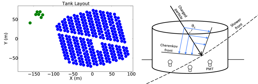
Figure 11: HAWC layout and operation principle. Left: HAWC tank layout. Right: Sketch of Water Cherenkov Detection Principle. From [10].

4 Towards large scale, worldwide observatories

4.1 Challenges

While the VHE gamma-ray instruments have matured they faced new challenges. The first is the amount of data that is being taken and needs to be processed and archived. While the duty cycle of HESS, MAGIC or VERITAS is about 1200 h per year (which does not seem to be large), they record some 200-400 TB per instrument per year. For the life time of an experiment (about 10 years is foreseen) it becomes several Petabytes of data. This made the use of distributed computing and large data centers an essential point in cost, but also in successful operation of the instruments.

The second challenge is the automation of the telescope operation. The observer teams are still required to be on-site to take shifts of data taking but the instruments are so complex and the operation duty cycle is so demanding that it became impossible to educate every observer on shift with many technical details of the instruments. To ensure stable operation and reduce human errors, the automation of the operation is implemented and the role of the observers is mainly to react in case automatic procedures fail.

The third challenge is the automation of the data processing. The amount of data mentioned earlier is so large that it cannot be processed manually. Automatic pipelines for data quality, data calibration, low level image parameter calculation as well as for high level products such as sky maps and energy spectra are implemented. Team of experts are overlooking the pipelines to react on possible exceptions and problems but this must be well organized to reduce the manpower needed.

4.2 Building a new community

There is an increasing demand on close cooperation between different VHE collaborations on several scientific topics, particularly with the HE community (space-borne detectors). Shared efforts for monitoring variable sources and maximizing time coverage of flaring known sources are some of the examples of good cooperation. In the extragalactic sky, joint campaigns on the radio galaxy M 87 discovering a day-scale VHE gamma-ray variability is the best example. In the Galaxy, joint campaigns on gamma-ray binary LS I+61 303 trying to unveil the reason for a super-orbital modulation of the emission is another good example.

Though positive examples exist, large collaborations and their rather strict data access and publication rights make joint publication a complicated and rather time-consuming process. Experts that are non-collaboration members do not have access to IACT low level products and are usually discouraged by the size of the collaborations and the complexity of the data processing. Therefore, a call for a different organization of IACTs, such as is common at optical observatories, with open calls for observation proposals and data rights either partially or completely public, gains a large popularity. Operating IACTs as open observatories, implying public data analysis tools and data archives accessible to general astronomers, would necessarily increase the scientific output of the observations through a participation of astronomers and astrophysicists that are experts on the research field but non-experts of the IACT data analysis.

Publication of scientific results becomes another challenge. At the beginning of the successful era of the VHE gamma-ray community every gamma-ray source detection was a great discovery leading to a publication. Nowadays, and probably even more after the advent of CTA, a well organized multi-wavelength campaign generally needs to be conducted and detailed studies of the source behavior performed to learn something significantly new. While the discovery potential of the instruments is still high (e.g. only about 5% of the extragalactic sky were observed with IACTs so far) the effort to produce a scientific publication of the high standard increases. The publication policy of major IACTs typically requires that the entire collaboration (100-150 people) sign every scientific publication, in order to acknowledge the high effort of individuals in instrument construction and operation. With the increase of collaboration sizes, this model might lead to unacceptable delays and may need to be revised.

4.3 Cherenkov Telescope Array

What was not possible in 1992 [34], became reality around 2006. A community-driven effort resulted in unifying major European, American, and Japanese groups from H.E.S.S.  MAGIC and VERITAS to design a large scale Cherenkov telescope observatory. The maturity of the current big experiments and the need for larger financial resources to significantly improve the sensitivity of the instruments led to a consolidation of the efforts for the next generation instrument.

The Cherenkov Telescope Array (CTA) was born as an idea for two observatories, one in each hemisphere, and to cover energies from 10s of GeV to 100s of TeV with unprecedented sensitivity. The project was funded for the design phase of 5 years in 2008.

At the moment, CTA brings together a community of more than 1500 scientists from all over the world, with groups in Europe, Asia, North and South-America, Africa, and Australia. The collaboration is presently nearly ready to start the construction of more than 150 telescopes.

The optimization process of the array layout (in terms of cost and sensitivity) favors usage of three different telescope types on the same site: few large size telescopes (LSTs), some 15-25 mid size telescopes (MSTs), and many (order of 70) small size telescopes (SSTs). For low gamma-ray energies, the major task is to collect every single Cherenkov photon from faint air-showers. This motivates usage of LSTs: four $23\mathrm{\ m}$ diameter parabolic dish telescopes with a field of view of $4.5^{\circ}$. The physics of transient phenomena, such as very-high-energy counterparts of Gamma Ray Bursts, requires fast slewing telescopes which limits the camera weight and therefore prevents the usage of a larger field of view. LSTs, which essentially follow the MAGIC design with a light weight structure, are most sensitive between $20\mathrm{\ GeV}$ and few TeV. The MSTs are an optimization result of HESS-1 (camera and trigger) and VERITAS (mount) telescopes and target the golden energy regime of IACTs around $1\mathrm{\ TeV}$. With $12\mathrm{\ m}$ diameter Davies-Cotton reflector, fine-grained cameras and fields of view larger than $7^{\circ}$, MSTs will have an improved survey capability. The number of MSTs is optimized to obtain multiple ($>4$) images from the same shower in the TeV range, which further improves the gamma-ray sensitivity. MSTs are most sensitive between $200\mathrm{\ GeV}$ and $50\mathrm{\ TeV}$. The SSTs are targeting gamma rays with energies above $20\mathrm{\ TeV}$, where detection and reconstruction is less a problem (the showers are rather luminous) but the expected fluxes are low. This motivates the construction of many SSTs in order to cover large area of up to $3\mathrm{\ km^{2}}$. Both SSTs and MSTs have dual mirror version prototypes, dubbed SST-dual mirror and Schwarzschild-Couder telescope respectively, which reduce camera sizes and encourage usage of small size advanced photo-sensors such as Silicon photomultipliers. The disadvantage of this design is the shadowing created by the secondary mirror, leading to a higher energy threshold which, however, is not critical due to the targeted energies at which showers contain a large amount of Cherenkov photons. A challenge of the dual-mirror technique is the precision of the mirror adjustment and control (at some critical points down to few tens of micrometers); the reward being an improved angular resolution and larger field of view.

Operating a “Hybrid” system, consisting of telescopes of different sizes, is however a complicated task. The observation strategy needs to be defined very precisely depending on the physics case (which telescope to use on a specific source, …), but also also at the reconstruction and analysis stage. HESS-II is currently the only hybrid system operating in the world. The data stream consists in both stereoscopic events (seen by at least two telescopes out of five) and monoscopic events (seen only by the large telescope). The analysis techniques are still under development to be able to cope with this much larger complexity, and this will become a real challenge for CTA. More and more accurate simulations are needed as new, more complex, detectors will come on line.

CTA will in general improve the sensitivity by an order of magnitude compared to what can be achieved with the current generation. Moreover it will extend the accessible energy range from $20\mathrm{\ GeV}$ (best overlap with gamma-ray satellites) to some 300 TeV (crucial for Pevatron searches). The cost of the project is about 300 M Euro and the construction phase should begin in 2016 with the goal to operate the full array by 2021. The sites of the CTA observatories have not yet been decided, with Chili and Namibia selected as Southern site candidates and Baja California (Mexico) and La Palma, Canary Islands (Spain) for the Northern site.

5 Outlook

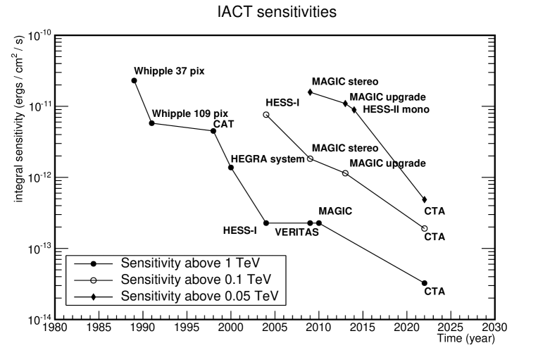
Figure 12: Evolution of integral sensitivity of the IACTs over time above 100 GeV (open circles) and 1 TeV (filled circles). The expected sensitivities of CTA are also shown. See text for references.

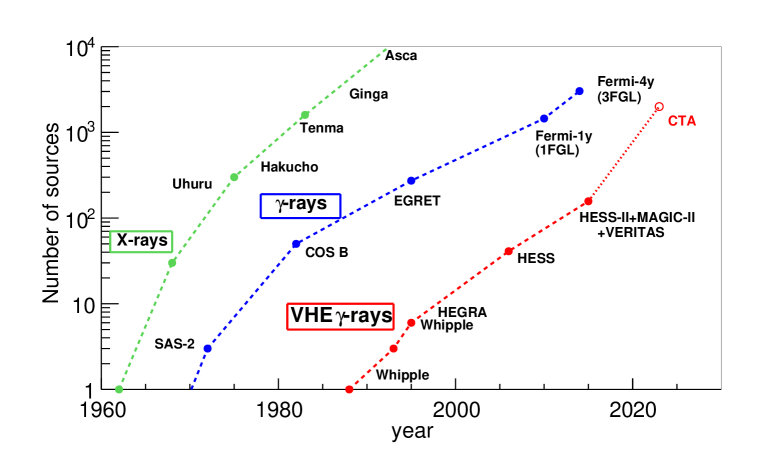
Figure 13: The so-called Kifune plot showing evolution of number of sources at different wavelengths as a function of time and different instruments. The CTA point is a prediction after 2 years data taking with two full arrays.

The IACT technique proved to be very efficient in detecting gamma-ray induced air showers and distinguishing them from the dominating background, mainly consisting of hadron-induced air showers. The evolution of the integral gamma-ray flux sensitivity for point sources is shown in Figure 12 as a function of time above three different thresholds: $50\mathrm{\ GeV}$, $100\mathrm{\ GeV}$ and $1\mathrm{\ TeV}$. The sensitivities are computed as Signal/sqrt(Background) for a 50 h observation for consistency with older experiments, even if this formula gives slightly overestimated results. The numbers are taken or computed from [4, 57, 35, 58, 59, 60, 61, 62] and are sometimes approximate. Since the first discovery of a VHE gamma-ray source (Whipple observatory, 1989), the sensitivity of the instruments at energies above $1\mathrm{\ TeV}$ improved by more than two orders of magnitude in less than 20 years. The sensitivity above $100\mathrm{\ GeV}$ improved by 1.5 orders of magnitude in 10 years. The extrapolation to the CTA era at all energies accessible by the IACTs clearly shows that the sensitivity potential of this technique is far from being saturated. In the $50\mathrm{\ GeV}$ to $1\mathrm{\ TeV}$ energy range, the expected sensitivities are almost an order of magnitude better than the ones of the current instruments all together.

By having such an enormous improvement in sensitivity in the IACT technique over the last 25 years there is no surprise that the number of detected sources at VHE should explode, too. In fact, the situation of the VHE gamma-ray astronomy is similar to the one of X-ray or lower energy gamma rays: there is almost an exponential rise of number of sources after a new window is opened in the electromagnetic spectrum, see Fig. 13. The so-called “Kifune-plot”, named after T. Kifune, who first showed a similar plot at the 1995 ICRC conference in Rome, shows that the number of detected sources does not saturate in the first 20-30 years and the CTA simulations follow this development. What this plot also shows is that for the time being the number of sources is not limited by their scarcity but by the sensitivity of the instruments. For many researchers, the recent success of VHE astronomy comes as a surprise, as in the 1980’s only a handful of them believed there was any detectable gamma-ray source above $100\mathrm{\ GeV}$.

References

- [1] Degrange, B. & Fontaine, G., gamma-ray astronomy / Astronomie des rayons gamma, Comptes Rendus Physique, 16 (6–7) (2015) 587 – 599.
- [2] Galbraith, W. & Jelley, J. V., Nat., 171 (1953) 349–350.
- [3] Blackett, P. M. S., in: The Emission Spectra of the Night Sky and Aurorae, (1948), p. 34.
- [4] Weekes, T. C., Cawley, M. F., Fegan, D. J., et al., The Astrophysical Journal, 342 (1989) 379–395.
- [5] de Naurois, M., Ph.D. thesis, Université Pierre et Marie Curie - Paris VI (2000).
- [6] Greisen, K., Progresses in Cosmic Ray Physics III (1956) .
- [7] Amenomori, M., Ayabe, S., Cao, P. Y., et al., The Astrophysical Journal, Letters, 525 (1999) L93–L96.
- [8] Aielli, G., Assiro, R., Bacci, C., et al., Nuclear Instruments and Methods in Physics Research Section A, 562 (1) (2006) 92 – 96.
- [9] Atkins, R., Benbow, W., Berley, D., et al., The Astrophysical Journal, 608 (2004) 680–685.
- [10] Abeysekara, A. U., Aguilar, J. A., Aguilar, S., et al., Astroparticle Physics, 35 (2012) 641–650.
- [11] Abeysekara, A. U., Alfaro, R., Alvarez, C., et al., Astroparticle Physics, 50 (2013) 26–32.
- [12] Auger, P., Ehrenfest, P., Maze, R., Daudin, J., & Fréon, R. A., Reviews of Modern Physics, 11 (1939) 288–291.
- [13] Cherenkov, P. A., Doklady Akademii Nauk SSSR, 2 (1934) 451.
- [14] Galbraith, W. & Jelley, J. V., Nature, 171 (1953) 349–350.
- [15] Weekes, T. C. & Turver, K. E., in: Wills, R. D. & Battrick, B. (Eds.), Recent Advances in Gamma-Ray Astronomy, Vol. 124 of ESA Special Publication, (1977), pp. 279–286.
- [16] Hillas, A. M., in: International Cosmic Ray Conference, (1985), pp. 445–448.
- [17] Fazio, G. G., Helmken, H. F., Rieke, G. H., & Weekes, T. C., Canadian Journal of Physics Supplement, 46 (1968) 451.
- [18] Lorenz, E. & Wagner, R., European Physical Journal H, 37 (2012) 459–513.
- [19] Weekes, T. C., in: International Cosmic Ray Conference, Vol. 8, (1981), p. 34.
- [20] Stepanian, A. A., Fomin, V. P., & Vladimirskii, B. M., Izvestiya Ordena Trudovogo Krasnogo Znameni Krymskoj Astrofizicheskoj Observatorii, 66 (1983) 234–241.
- [21] Vladimirsky, B. M., Zyskin, Y. L., Neshpor, Y. I., et al., in: Stepanian, A. A., Fegan, D. J., & Cawley, M. F. (Eds.), Very High Energy Gamma Ray Astronomy, (1989), p. 21.
- [22] Fomin, V. P., O’Flaherty, K. S., Kornienko, A. P., et al., International Cosmic Ray Conference, 2 (1991) 603.
- [23] Aharonian, F. A., Akhperjanian, A. G., Atoyan, A. M., et al., in: Stepanian, A. A., Fegan, D. J., & Cawley, M. F. (Eds.), Very High Energy Gamma Ray Astronomy, (1989), p. 36.
- [24] Nikolsky, S. I. & Sinitsyna, V. G., in: Stepanian, A. A., Fegan, D. J., & Cawley, M. F. (Eds.), Very High Energy Gamma Ray Astronomy, (1989), p. 11.
- [25] Kifune, T., in: Fleury, P. & Vacanti, G. (Eds.), Towards a Major Atmospheric Cerenkov Detector for TeV Astro/particle Physics, (1992), p. 229.
- [26] Aharonian, F. A., Akhperjanian, A. G., Kankanian, A. S., et al., International Cosmic Ray Conference, 2 (1991) 615.
- [27] Akerlof, C. W., Cawley, M. F., Fegan, D. J., et al., Nuclear Physics B Proceedings Supplements, 14 (1990) 237–243.
- [28] Bowden, C. C. G., Bradbury, S. M., Braier, K. T. S., et al., International Cosmic Ray Conference, 2 (1991) 626.
- [29] Goret, P., Palfrey, T., Tabary, A., Vacanti, G., & Bazer-Bachi, R., Astronomy & Astrophysics, 270 (1993) 401–406.
- [30] Baillon, P., Behr, L., Danagoulian, S., et al., (THEMISTOCLE Collaboration), Astroparticle Physics, 1 (1993) 341–355.
- [31] Aiso, S., Chikawa, M., Hayashi, Y., et al., International Cosmic Ray Conference, 3 (1997) 177.
- [32] Barrau, A., Bazer-Bachi, R., Beyer, E., et al., Nuclear Instruments and Methods in Physics Research A, 416 (1998) 278–292.
- [33] Punch, M., Akerlof, C. W., Cawley, M. F., et al., Nature, 358 (1992) 477.
- [34] Fleury, P. & Vacanti, G., in: Fleury, P. & Vacanti, G. (Eds.), Towards a Major Atmospheric Cerenkov Detector for TeV Astro/particle Physics, (1992).
- [35] Le Bohec, S., Degrange, B., Punch, M., et al., Nuclear Instruments and Methods in Physics Research A, 416 (1998) 425–437.
- [36] Chudakov, A. E., Dadykin, V. L., Zatsepin, V. I., & Nesterova, N. M., International Cosmic Ray Conference, 4 (1963) 199.
- [37] Paré, E., Balauge, B., Bazer-Bachi, R., et al., Nuclear Instruments and Methods in Physics Research A, 490 (2002) 71–89.
- [38] Gingrich, D. M., Boone, L. M., Bramel, D., et al., IEEE Transactions on Nuclear Science, 52 (2005) 2977–2985.
- [39] Tümer, T., Bhattacharya, D., Mohideen, U., et al., Astroparticle Physics, 11 (1999) 271–273.
- [40] Plaga, R., International Cosmic Ray Conference, 5 (1999) 215.
- [41] Atkins, R., Benbow, W., Berley, D., et al., Nuclear Instruments and Methods in Physics Research A, 449 (2000) 478–499.
- [42] Abdo, A. A., Allen, B., Berley, D., et al., The Astrophysical Journal, Letters, 664 (2007) L91–L94.
- [43] Hewitt, J. W. & Lemoine-Goumard, M., gamma-ray astronomy / Astronomie des rayons gamma, Comptes Rendus Physique, 16 (6–7) (2015) 674 – 685.
- [44] Dermer, C. & Giebels, B., this volume (2015) .
- [45] de Naurois, M., Habilitation thesis, Université Pierre et Marie Curie - Paris VI (2012).
- [46] Daum, A., Hermann, G., Hess, M., et al., Astroparticle Physics, 8 (1997) 1–11.
- [47] Reynolds, P. T., Akerlof, C. W., Cawley, M. F., et al., The Astrophysical Journal, 404 (1993) 206–218.
- [48] Mohanty, G., Biller, S., Carter-Lewis, D. A., et al., Astroparticle Physics, 9 (1998) 15–43.
- [49] Piron, P., this volume (2015) .
- [50] de Naurois, M. & Rolland, L., Astroparticle Physics, 32 (2009) 231–252.
- [51] Lemoine-Goumard, M., Degrange, B., & Tluczykont, M., Astroparticle Physics, 25 (2006) 195–211.
- [52] Naumann-Godó, M., Lemoine-Goumard, M., & Degrange, B., Astroparticle Physics, 31 (2009) 421–430.
- [53] de Naurois, M., ArXiv e-prints, astro-ph/0607247 (2006) .
- [54] HEGRA Collaboration, Heß, M., Bernlöhr, K., et al., Astroparticle Physics, 11 (1999) 363–377.
- [55] Aliu, E., Anderhub, H., Antonelli, L. A., et al., Astroparticle Physics, 30 (2009) 293–305.
- [56] Holder, J., in: International Cosmic Ray Conference, Vol. 5 of International Cosmic Ray Conference, (2005), p. 383.
- [57] Vacanti, G., Cawley, M. F., Colombo, E., et al., The Astrophysical Journal, 377 (1991) 467–479.
- [58] Pühlhofer, G., Bolz, O., Götting, N., et al., Astroparticle Physics, 20 (2003) 267–291.
- [59] Aharonian, F., Akhperjanian, A. G., Bazer-Bachi, A. R., et al., (H.E.S.S. Collaboration), Astronomy & Astrophysics, 457 (2006) 899.
- [60] Aleksić, J., Alvarez, E. A., Antonelli, L. A., et al., Astroparticle Physics, 35 (2012) 435–448.
- [61] Aleksić, J., Ansoldi, S., Antonelli, L. A., et al., Astroparticle Physics (2015) .
- [62] Bernlöhr, K., Barnacka, A., Becherini, Y., et al., Astroparticle Physics, 43 (2013) 171–188.