The hard-disk fluid revisited

Abstract

The hard-disk model plays a role of touchstone for testing and developing the transport theory. By large scale molecular dynamics simulations of this model, three important autocorrelation functions, and as a result the corresponding transport coefficients, i.e., the diffusion constant, the thermal conductivity and the shear viscosity, are found to deviate significantly from the predictions of the conventional transport theory beyond the dilute limit. To improve the theory, we consider both the kinetic process and the hydrodynamic process in the whole time range, rather than each process in a seperated time scale as the conventional transport theory does. With this consideration, a unified and coherent expression free of any fitting parameters is derived succesfully in the case of the velocity autocorrelation function, and its superiority to the conventional ‘piecewise’ formula is shown. This expression applies to the whole time range and up to moderate densities, and thus bridges the kinetics and hydrodynamics approaches in a self-consistent manner.

For a system with translation invariance, the transport theory predicts that the autocorrelation function (ACF) of a physical quantity, denoted by $C(t)$, generally decays as theorySP ; Lebowitz ; Leener ; Alder ; Alder2 ; Alder3 ; wain-tlnt ; Dorfman1 ; Dorfman2 ; Dorfman3 ; Ernst ; tlnt ; cv-longtail ; review-l-t-coupling ; high-density

$$\frac{C(t)}{C(0)}=\left\{\begin{array}[]{ll}e^{-\xi t},&\text{kinetics stage;}\\ b_{h}t^{-d/2},&\text{hydrodynamics stage.}\end{array}\right.$$ (1)

Here $t$ is the correlation time, $\xi$ is a characterizing constant, $d$ is the dimension of the system, $b_{h}$ is the amplitude of the power-law decay function. Given $C(t)$, the transport coefficient of the corresponding physical quantity can be obtained with the Green-Kubo formula theorySP ; Andrieux ; Kubo . The most important ACFs are those of the velocity, the energy current and the viscosity current, which will be referred to as the VACF, the EACF and the VisACF in the following.

Nevertheless, the transport theory has not been fully established. On one hand, the theoretical predictions have not been well verified yet. Though a lot of numerical studies have been done since the 1970’s Alder ; Alder2 ; wain-tlnt ; formula-2d ; 2d-tailnotimport ; Erpenbeck , the results are not accurate enough to conclude until 2008 pre2008 , Isobe computed the VACF of the two-dimensional hard-disk fluid and found that the tail is of the power-law $\sim t^{-1}$ at low densities but logarithmic $\sim(t\sqrt{\ln t})^{-1}$ at moderate densities. It implies that the power-law decay prediction may not be always correct. The logarithmic decay agrees with the self-consistent mode coupling prediction wain-tlnt ; tlnt . However, the transition form $\sim t^{-1}$ to $\sim(t\sqrt{\ln t})^{-1}$ has not been characterized. For the EACF and VisACF, up to now simulation results are rare and those allow for drawing a conclusion still lack. On the other hand, dividing the time dependence of $C(t)$ into the kinetics and hydrodynamics stages is an expedient measure. To quantitatively calculate the transport coefficient, a coherent and unified expression is indispensable. Particularly, for a two dimensional system the power-law tail of $C(t)$ makes the transport coefficient diverge in the thermodynamical limit, but for a real system, the measured coefficient should be finite. To predict the coefficient theoretically, one needs to evaluate the influence of the long-time tail to reveal when it can be ignored comparing with the kinetic contribution and when it becomes dominantformula-2d ; 2d-tailnotimport . This requires to know the crossover time from the kinetics stage to the hydrodynamics stage. Numerically, parameter fitting formula-2d ; pre2015 may allow one to construct a unified $C(t)$ within the time period investigated, but it is risky to extend it out or to use it in other parameter regimes.

In this work we revisit the hard-disk fluid. First, by large scale simulations, we calculate the three ACFs and show their deviations from the theoretical predictions. We then derive a unified expression for the VACF. The model consists of $N$ disks of unitary mass $m=1$ moving in an $L_{x}\times L_{y}$ rectangular area with the periodic boundary conditions. The system is evolved with the event-driven algorithm Alder ; cal at the dimensionless temperature $T=1$ (the Boltzmann constant is set to be $k_{B}=1$). The disk number density is fixing at $n=N/(L_{x}L_{y})=0.01$ throughout and the disk diameter, $\sigma$, is adopted to control the packing density $\phi=n\pi\sigma^{2}/4$ (referred to as the density for short in the following). Three cases, $\sigma=2$, $4$, and $6$ corresponding to $\phi\approx 0.03$, $0.13$, and $0.28$, respectively, are studied intensively. As a reference, the crystallization density is $\phi=0.71$, hence our study covers the moderate density regime. Applying the Enskog formula with the first Sonine polynomial approximation formula-2d ; Gass ; pl-eskog , the diffusion coefficient $D$, the thermal conductivity $\lambda$, the sheer viscosity $\eta$, and the sound speed $u_{s}$ are, respectively, $D=13.4$, $5.70$, $2.76$, $\lambda=0.59$, $0.35$ , $0.36$, $\eta=0.14$, $0.077$, $0.063$, and $u_{s}=1.5$, $1.8$, $2.7$, for the three densities.

The VACF is defined as $C_{u}(t)=$ $\langle u_{x}(t)u_{x}(0)\rangle$, where $u_{x}(t)$ is the $x$-component of the velocity of a tagged disk. Figure 1(a)-(c) show the simulated results obtained with $10^{10}$ ensemble samples for $L_{x}=L_{y}=2000$ ($N=40000$). The time range free from the finite-size effects is $0\leq t<t_{f}=L_{x}/(2u_{s})$ pre2008 ; chenfinite ; SM . For the three densities, $t_{f}=667$, $556$, and $370$, respectively. In this time range, the initial exponential decaying stage and the long-time tail can be observed in all the three cases. The hydrodynamics prediction $C_{u}(t)/C_{u}(0)=[8\pi(D+\nu)n]^{-1}t^{-1}$ Alder ; Alder2 ; Alder3 ; wain-tlnt ; Dorfman1 ; Dorfman2 ; Dorfman3 is also plotted for comparison, where $\nu=\eta m/n$ is the viscosity diffusivity. It can be seen that the predicted $\sim t^{-1}$ tail is close to the simulation result, but as the density increases, the deviation grows. The diffusion coefficients calculated following the Green-Kubo formula, $D(t)=\int_{0}^{t}C_{u}(t^{\prime})dt^{\prime}$, are shown in Fig. 1(d).

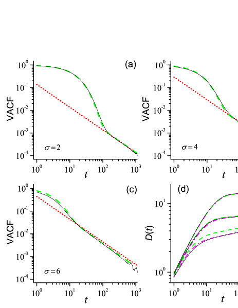
Figure 1: (Color online) (a)-(c) The VACFs obtained by, respectively, simulations (black solid lines), the unified formula Eq. (5) (green dashed lines), and the hydrodynamics theory (red dotted lines). (d) The diffusion coefficients calculated with the VACFs obtained by simulations (black solid lines) and by the unified formula Eq. (5). For the latter, the green dashed lines are for the results with the kinetic transport coefficients given by the Enskog equation and the magenta dash-dotted lines are for the results with the corrected coefficients.

Calculating the EACF $C_{J}(t)=\langle J_{x}(t)J_{x}(0)\rangle$ is $N$ times harder than calculating the VACF. Here $J_{x}(t)=\sum_{i}j_{x}^{i}(t)$, where $j_{x}^{i}(t)=|\mathbf{v}^{i}|^{2}v_{x}^{i}$ is the $x$-component of the energy current of the $i$th disk. For a given simulation run we can obtain $N$ ensemble samples for calculating $C_{u}(t)$ as every disk can be taken as the tagged disk but only one for calculating $C_{J}(t)$ because the total current, $J_{x}$, involves the contributions of all the disks wain-tlnt ; tlnt . This is the reason why the hydrodynamics prediction of the EACF has not been conclusively tested. To decrease the simulation difficulty we consider a smaller size, i.e., $L_{x}\times L_{y}=3000\times 400$ $(N=12000)$. Correspondingly, $t_{f}=1000$, $833$, and $535$ for the three densities. Figure 2(a)-(c) show the results of $C_{J}(t)$ calculated with $10^{9}$ ensemble samples. For $\sigma=2$, a perfect $\sim t^{-1}$ tail is observed, but the value of $C_{J}(t)$ at the tail is one time larger than the hydrodynamics prediction Alder ; Alder2 ; Alder3 ; wain-tlnt ; Dorfman1 ; Dorfman2 ; Dorfman3 that $C_{J}(t)/C_{J}(0)=[4\pi(\eta/m+\lambda/2k_{B})]^{-1}t^{-1}$. For $\sigma=4$ and $6$, the EACF shows a multistage decaying behavior – after the initial exponential decaying stage there appears another fast decaying stage, before a power-law tail slower than $\sim t^{-1}$ follows. Figure 2(d) shows the corresponding thermal conductivity calculated following the Green-Kubo formula $\lambda(t)=\frac{1}{k_{B}T^{2}L_{x}L_{y}}\int_{0}^{t}C_{J}(t^{\prime})dt^{\prime}$.

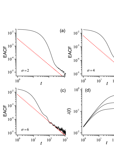
Figure 2: (Color online) (a)-(c) The EACFs obtained by simulations (black solid lines) and by the hydrodynamics theory (red dotted lines). (d) The thermal conductivity calculated based on the EACFs obtained by simulations.

Calculating the VisACF $C_{vis}(t)=\langle J_{vis}(t)J_{vis}(0)\rangle$ suffers from the same difficulty. Here $J_{vis}(t)=\sum_{i}u_{x}^{i}(t)u_{y}^{i}(t)$. Taking $L_{x}=L_{y}=1000$ $(N=10^{4})$ and $\sigma=4$, we show in Fig. 3(a) the VisACF calculated with $10^{10}$ ensemble samples. Though for $t<t_{f}=278$ the VisACF decays fast for several orders, it is still uncertain if a power-law tail follows. Indeed, the VisACF may drop to be negative from $t\approx 70$ to $100$. The demanded huge amount of samples make the computation so difficult that we can only provide the results for one case ($\sigma=4$) as an example. The hydrodynamics prediction $C_{vis}(t)/C_{vis}(0)=(32\pi)^{-1}[m/\eta+(\eta/m+\lambda/2k_{B})^{-1}]t^{-1}$ Alder ; Alder2 ; Alder3 ; wain-tlnt ; Dorfman1 ; Dorfman2 ; Dorfman3 is also plotted for comparison. Figure 3(b) shows the shear viscosity by following the Green-Kubo formula $\eta(t)=m\int_{0}^{t}C_{vis}(t^{\prime})dt^{\prime}$.

Figure 3: (Color online) (a) The simulation result of the VisACF and (b) the corresponding sheer viscosity for $\sigma=4$.

Next, we derive the unified expression for the VACF. Our key consideration is that the VACF is governed by two physical processes simultaneously. One is collisions of the tagged disk with other surrounding disks, referred to as the kinetic process, through which $C_{u}(0)$ will be transferred to other disks from the tagged disk. Let $C_{u}^{k}(t)$ denote the portion of $C_{u}(0)$ that has not been transferred at time $t$. Following the kinetics theory, it decays exponentially: $C_{u}^{k}(t)=C_{u}(0)\exp({-\frac{k_{B}T}{mD^{k}}t})$ Alder ; Alder2 ; Alder3 ; Dorfman1 ; Dorfman2 ; Dorfman3 , where $D^{k}$ is the kinetic diffusion constant. Meanwhile, it is possible for the transferred portion to feedback to the tagged disk by ring collisionsAlder2 , which is referred to as the hydrodynamic process. The amount returns to the tagged disk at time $t$, denoted by $C_{u}^{h}(t)$, contributes to the hydrodynamics diffusion constant $D^{h}$. The VACF is thus a sum of these two portions,

$$C_{u}(t)=C_{u}^{k}(t)+C_{u}^{h}(t),$$ (2)

and the diffusion constant is divided into the kinetic and hydrodynamic parts as $D=D^{k}+D^{h}$ accordingly. To obtain $C_{u}^{h}(t)$, it is necessary to investigate how $C_{u}(0)$ is delivered to the surroundings. This reduces to investigating the relaxation process of the momentum $\mathbf{p}_{c}=m\mathbf{u}_{c}$ initially carried by the tagged disk, which can be approached with the spatiotemporal correlation function zhao2006 ; chendiffusion

$$c(\mathbf{r},t)=\frac{\langle\mathbf{p}_{c}\cdot\mathbf{p}(\mathbf{r},t)\rangle}{\langle|\mathbf{p}_{c}|^{2}\rangle}+\frac{n}{N-1}.$$ (3)

Here $\mathbf{p}(\mathbf{r},t)$ is the momentum density of the system. It is found that $c(\mathbf{r},t)$ is axisymmetric with respect to $\mathbf{r}=0$; it has one center peak surrounded by a ‘crater’ (see Fig. 4(a)-(b) for the intersection of $c(\mathbf{r},t)$ with $y=0$) and the center peak can be well fitted by the Gaussian function $c^{center}(\mathbf{r},t)=\frac{a_{\nu}}{4\pi\widetilde{\nu}t}\exp({-\frac{r^{2}}{4\widetilde{\nu}t}})$ with $a_{\nu}=1/2$ and $\widetilde{\nu}=14.3$, $8.3$, and $7.9$ for $\sigma=2$, $4$, and $6$, respectively. The function $c(\mathbf{r},t)$ gives the portion of $C_{u}(0)$, that transfers to a unit area centering $\mathbf{r}$ at time $t$. There are $n$ disks on average in this area, and each of them carries a portion, i.e., $c(\mathbf{r},t)/n$, of $C_{u}(0)$. Suppose that the tagged disk appears in this area with the probability $\rho(\mathbf{r},t)$, then on average the portion of $C_{u}(0)$ it carries is $\rho(\mathbf{r},t)c(\mathbf{r},t)/n$. The total amount carried by it is therefore $C_{u}^{h}(t)=(1/n)C_{u}(0)\int c(\mathbf{r},t)\rho(\mathbf{r},t)d\mathbf{r}$.

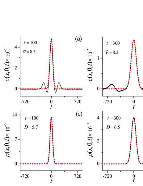
Figure 4: (Color online) (a)-(b) The intersection of $c(\mathbf{r},t)$ and (c)-(d) the intersection of $\rho(\mathbf{r},t)$ at $t=100$ and $300$ (black solid lines). The red dotted line in each panel is the best Gaussian fitting to the center peak of $c(\mathbf{r},t)$ or $\rho(\mathbf{r},t)$. $\sigma=4$.

The probability function $\rho(\mathbf{r},t)$ can be measured directly by tracing the tagged disk. It is found to overlap perfectly with a Gaussian function (see Fig. 4(c)-(d) for its intersection) with a time dependent diffusion coefficient, i.e., $\rho(\mathbf{r},t)=\frac{1}{4\pi D(t)t}\exp({-\frac{r^{2}}{4D(t)t}})$. As $\rho(\mathbf{r},t)$ decays exponentially as $r^{2}$, we can replace $c(\mathbf{r},t)$ with $c^{center}(\mathbf{r},t)$ in the integrand for calculating $C_{u}^{h}(t)$. With this simplification we have

$$C_{u}^{h}(t)/C_{u}(0)=a_{\nu}[4\pi(D(t)+\widetilde{\nu})n]^{-1}t^{-1}.$$ (4)

Noting that Fig. 4 represents the case that the hydrodynamics effects become completely dominant. For $t>100$, $C_{u}^{k}(t)$ has decayed to a negligibly small value($<10^{-8}$ with $D^{k}=5.70$), implying that $C_{u}(0)$ has transferred to the surrounding disks almost completely. Equation (4) thus characterizes the situation at large times. At short times, the portion of $C_{u}(0)$ the hydrodynamics process accounts for is $C_{u}(0)[1-\exp(-\frac{k_{B}T}{mD^{k}}t)]$; Assuming that $c(\mathbf{r},t)$ for this portion has the same structure as shown in Fig. 4(a)-4(b), it is straightforward to have

$$C_{u}^{h}(t)/C_{u}(0)=a_{\nu}[1-\exp(-\frac{k_{B}T}{mD^{k}}t)][4\pi(D(t)+\widetilde{\nu})n]^{-1}t^{-1}.$$ (5)

This extended expression applies in both the kinetics and the hydrodynamics stages.

The parameter $a_{v}$ and $\widetilde{\nu}$ can be connected to the properties of the hydrodynamic modes analytically  SM . Let $n(\mathbf{r},t)$ and $\mathbf{u}(\mathbf{r},t)$ be the disk number density and the velocity density, we have $\mathbf{p}(\mathbf{r},t)=mn(\mathbf{r},t)\mathbf{u}(\mathbf{r},t)=m\mathbf{j}(\mathbf{r},t)$, considering the hydrodynamics assumption theorySP that local deviations of hydrodynamic variables from their average values are small. Here $\mathbf{j}(\mathbf{r},t)$ is the local disk current. Applying the hydrodynamics analysis to solve the linearized conservation laws for the disk number, the energy, and the momentum with initial conditions of $\delta$-function impulses of $\delta(\mathbf{r})\Delta n$, $\delta(\mathbf{r})\Delta T$ and $\delta(\mathbf{r})\mathbf{p}_{c}$, we obtain $c(\mathbf{k},t)=(k_{y}^{2}/k^{2})\exp(-\nu k^{2}t)$ in the wave-vector space, where $\Delta n$ and $\Delta T$ represent the deviation of the disk density and the temperature induced by the tagged particle, and $\mathbf{k}$ is the wave vector in the Fourier space. With a rough estimation of $k_{y}^{2}/k^{2}\sim 1/2$, it appears $c(\mathbf{k},t)=(1/2)\exp(-\nu k^{2}t)$ and gives $c(\mathbf{r},t)=(1/8\pi\nu t)\exp(-r^{2}/4\nu t)$ in the real space. The expression of $c(\mathbf{r},t)$ implies $a_{v}=1/2$ and $\widetilde{\nu}=\nu$. With this connection, Eq. (4) is exactly the same as that of the hydrodynamics theory.

In principle, $\nu$ is time-dependent according to the hydrodynamics theory, but based on our numerical observation of the relaxation of $c^{center}(\mathbf{r},t)$ and the fact that $\eta$ converges in time [see Fig. 3(d)], it can be assumed to be a time-independent constant up to moderate densities. Previous numerical studies using the Helfand-Einstein formula have also shown that the shear viscosity does not depend on the system size either formula-2d ; 2d-tailnotimport , which supporting the constant $\nu$ assumption as well.

Inserting $C_{u}^{h}(t)$ into the Green-Kubo formula, we have

$$D^{h}(t)=\int_{0}^{t}C_{u}^{h}(t^{\prime})dt^{\prime}.$$ (6)

It is interesting to note that the self-consistent solutions wain-tlnt ; tlnt , i.e., $C_{u}^{h}(t)/C_{u}(0)=\sqrt{1/16\pi n}(t\sqrt{\ln(t)})^{-1}$ and $D^{h}(t)=\sqrt{k_{B}T\ln(t)/4\pi mn}$, are asymptotic solutions of Eq. (5) and (6) in the long-time limit where $D^{h}(t)\gg D^{k}+\nu$, i.e., $t>\exp[(4\pi mn/k_{B}T)(D^{k}+\nu)^{2}]$. Using the Enskog results of $D^{k}$ and $\nu$, it can be estimated that this time scale is about $10^{23}$, $10^{10}$, and $10^{4}$, respectively, for $\sigma=2$, $4$, and $6$. During the transition process which may contribute a dominant part to the diffusion constant, the self-consistent asymptotic solutions are not exact.

In order to solve the coupled equations (5) and (6) accurately, we turn to the iterative algorithm: We set $D^{h}(t)=0$ as the first trial solution and substitute it into Eq. (5) to get $C_{u}^{h}(t)$, then put it into Eq. (6) to get the next trial solution of $D^{h}(t)$, and so on. In general if $D^{h}(t)$ increases, $C_{u}^{h}(t)$ will decrease and make $D^{h}(t)$ decrease, and vice versus, hence the convergence of the iteration is guaranteed. Indeed, usually the solutions converge after only several iterations. The predicted VACFs [Fig.1(a)-(c)] and the corresponding diffusion coefficients [Fig.1(d)] agree with the simulation results quite well, except that the diffusion coefficient $D(t)$ show a shift from the simulation result as the density increases.

This deviation should be induced by the inaccuracy of the kinetics transport coefficients that we have employed. With the simulation data of $C_{u}(t)$, we can estimate the kinetics diffusion constant $D^{k}$. The kinetics process plays a role mainly before the time, denoted as $\tau$, at which $C_{u}(t)$ turns from the exponential decay to the followed tail. For example, for $\sigma=2$, $\tau\approx 110$, at which $C_{u}^{k}$ has decayed to $C_{u}^{k}(\tau)/C_{u}(0)\sim 10^{-4}$. Truncating the Green-Kubo integration at $\tau$, we have $D(\tau)=13.97$, $6.40$, and $2.85$ for $\sigma=2$, $4$, and $6$, respectively. These values can be considered as the upper bound of $D^{k}$. Subtracting $D^{h}(\tau)$ from it, we get the estimated $D^{k}$; i.e., $D^{k}=13.61$, $5.50$, and $2.35$, correspondingly. These values are close to the Enskog approximations, within maximally $13\%$ errors. Meanwhile, the relation $\widetilde{\nu}=\nu$ is also not accurate; it is a result of ignoring the anisotropic feature of the momentum diffusion SM . More properly, $\widetilde{\nu}$ measured by the direct simulation should be employed to characterize the momentum diffusion instead of $\nu$. With these corrections of $D^{k}$ and $\nu$, the shift of $D(t)$ can be well suppressed [see Fig. 1(d)].

Similarly, we can estimate the upper bounds for the heat conductivity. From Fig. 2(d) we have the heat conductivity $\lambda\leq 0.580$, $0.258$, and $0.139$ for $\sigma=2$, $4$, and $6$, respectively, which deviates at least $2\%$, $36\%$, and $160\%$ from the Enskog approximations. Therefore, the Enskog equation is relatively precise for the kinetic diffusion constant, but lacks accuracy for the heat conductivity and the sheer viscosity at higher densities.

With the unified expression of $C_{u}(t)$, we can estimate the hydrodynamics contribution to the diffusion constant to systems of macroscopic sizes. For example, the average distance between two neighboring molecules in the air is about $10^{-9}$ meter, implying that if our model has a macroscopic size, say one centimeter, we have $L_{x}$, $L_{y}\sim 10^{8}$. For such a size, the time a disk diffuses freely without being influenced by the boundaries is $t\sim L_{x}/(2u_{s})\sim 10^{7}$. Taking this time as the truncation time of integration in Eqs. (5) and (6), our iteration algorithm gives $D^{h}(t)/D^{k}\approx 0.15$, $0.5$, and $10$ for $\sigma=2$, $4$,and $6$, respectively, suggesting that in a dilute system it is the kinetics contribution that dominates, but as the density increases, the hydrodynamics contribution increases dramatically and the kinetics contribution turns to be negligible.

In summary, beyond the dilute limit, the accuracy of the hydrodynamics theory is not sufficient in describing the ACFs at least in the transient stage that is essential for calculating the transport coefficients. For the VACF, the numerically observed tail is between $\sim t^{-1}$ and $\sim(t\sqrt{\ln(t)})^{-1}$. For the EACF, we have evidenced the power-law tail but the exponent agrees with the hydrodynamics prediction only in a very dilute system. As the density increase, a multistage decaying phenomenon is observed, and the long-time tail is slower than $\sim t^{-1}$. The VisACF decays much faster than the VACF and the EACF. The long-time tail has not been observed in our example. In addition, we have estimated the upper bounds of transport coefficients using the simulated ACFs, and reveal that the Enskog equation generally used for approximating the kinetics transport coefficients need be improved particularly at higher densities.

For the VACF, our intuitive representation of the ring-collision mechanism and the iterative algorithm lead us to a unified and coherent expression valid in the whole time range. The key point is to distinguish the kinetics and the hydrodynamics processes and investigate them respectively over the whole time range. Particularly, we emphasize that the hydrodynamic contribution at short times should not be ignored. This is different from the traditional treatments that divide the relax process into separated stages. Extension of our method to the EACF and VisACF is open.

Acknowledgments

Very useful discussions with J. Wang, Y. Zhang and Dahai He are gratefully acknowledged. This work is supported by the National Natural Science Foundation of China (Grant No. 11335006), and the NSCC-I computer system of China.

References

- (1) J. P. Hansen and I. R. McDonald, Theory of Simple Liquids, 3rd ed. (Academic, London, 2006).
- (2) F. Bonetto, J. L. Lebowitz, and L. Rey-Bellet, Fourie’s Law: A Chanllenge to Theorists, Mathematical Physics 2000 (Imperial College Press, London, 2000).
- (3) P. Reusibois and M. de Leener, Classical Kinetic Theory of Fluids Wiley-Interscience, New York, 1977.
- (4) B. S. Alder and T. E. Wainwright, Phys. Rev. Lett. 18, 988 (1967)
- (5) B. S. Alder and T. E. Wainwright, Phys. Rev. A 1,18 (1970).
- (6) B. S. Alder, D. M. Gass, and T. E. Wainwright, J. Chem. Phys. 53, 3813 (1970).
- (7) T. E. Wainwright, B.J. Alder, and D. M. Gass, Phys. Rev. A 4, 233 (1971).
- (8) S. R. Dorfman and E. G. D. Cohen, Phys. Rev. Lett. 25, 1257(1970)
- (9) J. R. Dorfman and E. G. D. Cohen, Phys. Rev. A 6, 776 (1972)
- (10) S. R. Dorfman and E. G. D. Cohen, Phys. Rev. A.12, 292 (1975).
- (11) M. H. Ernst, E. H. Hauge, and J. M. J. van Leeuwen, Phys. Rev. A 4, 2055 (1971)
- (12) D. Forster, D. R. Nelson, and M. J. Stephen, Phys. Rev. A 16 732 (1977).
- (13) J. J. Erpenbeck and W. W. Wood, Phys. Rev. A 26, 1648 (1982); Phys. Rev. A 32, 412 (1985).
- (14) Y. Pomeau and P. Reuibois, Physics Reports, 19, 63 (1975).
- (15) J. W. Dufty, Mol. Phys. 100, 2331, (2002); J. W. Dufty and M. H. Ernst, ibid, 102, 2123 (2004).
- (16) R. Kubo, M. Toda, and N. Hashitsume, Statistical Physics II: Nonequilibrium Statistical Mechanics (Springer, New York, 1991);
- (17) D. Andrieux and P. Gaspard, J. Stat. Mech. P02006 (2007).
- (18) R. Garcia-Rojo, S. Luding, and J. J. Brey, Phys. Rev. E 74, 061305 (2006).
- (19) S. Viscardy and P. Gaspard, Phys. Rev. E 68, 041204 (2003).
- (20) J. J. Erpenbeck and W. W. Wood, Phys. Rev. A 26, 1648(1982)
- (21) M. Isobe, Phys. Rev. E 77, 021201 (2008).
- (22) S. Bellissima, M. Neumann, E. Guarini, U. Bafile, and F. Barocchi, Phys. Rev. E 92, 042166 (2015).
- (23) D. C. Rapaport, J. Comput. Phys. 34, 184 (1980)
- (24) D. M. Gass, J. Chem. Phys. 54, 1898 (1971).
- (25) J. J. Erpenbeck and W. W. Wood, Phys. Rev. A 43, 4254 (1991).
- (26) S. Chen, Y. Zhang, J. Wang, and H. Zhao, Phys. Rev. E 89, 022111 (2014)
- (27) S. Chen, Y. Zhang, J. Wang, and H. Zhao, J. Stat. Mech., 033205 (2016)
- (28) H. Zhao, Phys. Rev. Lett. 96, 140602 (2006)
- (29) S. Chen, Y. Zhang, J. Wang, and H. Zhao, Phys. Rev. E 87, 032153 (2013)
- (30) See the Supplied Materials with this submission.