Understanding frequency distributions of path-dependent processes with non-multinomial maximum entropy approaches

Abstract

Path-dependent stochastic processes are often non-ergodic and observables can no longer be computed within the ensemble picture. The resulting mathematical difficulties pose severe limits to the analytical understanding of path-dependent processes. Their statistics is typically non-multinomial in the sense that the multiplicities of the occurrence of states is not a multinomial factor. The maximum entropy principle is tightly related to multinomial processes, non-interacting systems, and to the ensemble picture; It loses its meaning for path-dependent processes. Here we show that an equivalent to the ensemble picture exists for path-dependent processes, such that the non-multinomial statistics of the underlying dynamical process, by construction, is captured correctly in a functional that plays the role of a relative entropy. We demonstrate this for self-reinforcing Polya urn processes, which explicitly generalise multinomial statistics. We demonstrate the adequacy of this constructive approach towards non-multinomial pendants of entropy by computing frequency and rank distributions of Polya urn processes. We show how microscopic update rules of a path-dependent process allow us to explicitly construct a non-multinomial entropy functional, that, when maximized, predicts the time-dependent distribution function.

Keywords: Pólya urns, statistical mechanics, maximum entropy principle, relative entropy, information divergence

1 Introduction

“It seems questionable whether the Boltzmann principle alone, meaning without a complete […] mechanical description or some other complementary description of the process, can be given any meaning.” Einstein’s famous critical comment on the completeness of Boltzmann entropy, [1], is still thought provoking. For ergodic systems, e.g. [2], over a well defined set of states, this critique has turned out to be of minor relevance. Here we demonstrate how Einstein’s observation becomes relevant again when dealing with non-ergodic, path-dependent systems or processes, i.e. processes where ensemble and time averages cease to yield identical results and the ensemble descriptions of a processes fails to describe the dynamics of a particular process (e.g. compare [3]).

Moreover, for path dependent systems we have to specify what we mean with “entropy”, since no unique generalization of entropy from equilibrium to non-equilibrium systems exists. However, Boltzmann’s principle is grounded in the idea that in large systems the most likely samples we may draw from a process, i.e. the so called maximum-configuration, also characterize the typical samples, while it becomes very unlikely to draw atypical samples. In fact we will demonstrate the possibility to directly construct “entropic functionals” from the microscopic properties determining the dynamics of a large class of non-ergodic processes using maximum-configuration frame work. In this approach we identify relative entropy (up to a multiplicative constant) with the logarithm of the probability to observe a particular macro state (which typically is represented by a histogram over a set of observables states), compare e.g. [4]. By construction, maximisation of the resulting entropy functionals leads to adequate predictions of statistical properties of non-ergodic processes, in maximum configuration.

For ergodic processes it is possible to replace time-averages of observables by their ensemble-averages, which leads to a tremendous simplification of computations. In particular, this is true for systems composed of independent particles or for Bernoulli processes, i.e. processes where samples are drawn independently, and the states of the independent components or observations collectively follow a multinomial statistics. The multinomial statistics of such a system with $W$ observable states $i=1,\cdots,W$ is captured by a functional that coincides with Shannon entropy [5], $H(p)=-\sum_{i=1}^{W}p_{i}\log p_{i}$. In this context $p=(p_{1},\cdots,p_{W})$ is the empirical relative frequency distribution of observing states $i$ in an experiment of drawing from the process for $N$ times, i.e. $p=k/N$ is the normalized histogram of the experiment where state $i$ has been drawn $k_{i}$ times. Clearly, $\sum_{i}k_{i}=N$. In this context $H(p)$ can be understood as the logarithm of the multinomial factor, i.e. $-\sum_{i=1}^{W}p_{i}\log p_{i}\sim\frac{1}{N}\log{N\choose k}$, where and ${N\choose{k}}=N!/\prod_{i=1}^{W}k_{i}!$ (e.g. compare [6]).

Maximization of Shannon entropy under constraints therefore is a way of finding the most likely relative frequency distribution function (normalized histogram of sampled events) one will observe when measuring a system, provided that it follows a multinomial statistics. Constraints represent knowledge about the system. Bernoulli processes with multinomial statistics are characterized by the prior probabilities, $q=(q_{1},\cdots,q_{W})$. In general, the set of parameters characterizing a process, we denote by $\theta$. In the multinomial case $\theta\equiv q$.

Denoting the probability to measure a specific histogram by $P(k|\theta,N)$, the most likely histogram $\hat{k}$, that maximizes $P(k|\theta,N)$, is the optimal predictor or the so-called maximum configuration. For a multinomial distribution function, $P(k|\theta,N)={N\choose{k}}q_{i}^{k_{i}}$, where $q_{i}$ are the prior probabilities (or biases), the functional that is maximized is $\psi(p|\theta)=H(p)+\sum_{i}p_{i}\log q_{i}$, which is (up to a sign) called the relative entropy or Kullback-Leibler divergence [7]. The term $H(p)$ coincides with Shannon entropy, the term that depends on $q$ is called cross-entropy and is a linear functional in $p$. By re-parametrizing $q_{i}=\exp(-\beta\varepsilon_{i})$, where $\beta>0$ is a constant, one gets the standard max-ent functional

$$\psi(p|\theta,N)=H(p)-\beta\sum_{i}p_{i}\varepsilon_{i}\qquad\left[\sum_{i}p_{i}=1\right]\quad.$$ (1)

In statistical physics, the constants $\varepsilon_{i}$ typically correspond to energies and $\beta$ to the so called inverse temperature of a system. Maximization of this functional with respect to $p$ yields the most likely empirical distribution function; this is sometimes called the maximum entropy principle (MEP).

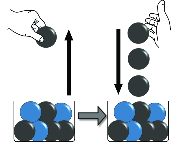
Figure 1: Schematic illustration of a Pólya process. When a ball of a certain color is drawn, it is replaced by $1+\delta$ balls of the same color. Then the next ball is drawn and the process is repeated for $N$ iterations. Here $\delta=2$. This reinforcement process creates a history-dependent dynamics. The configurations obtained after successive iterations have non-multinomial structure.

Clearly, systems composed of independent components follow a multinomial statistics. Note that a multinomial statistics is also a direct consequence of working with ensembles of statistically independent systems. In this case the multinomial distribution function reflects the ensemble property and is not necessarily a property of the system itself. Therefore $H(p)$ only has physical relevance for systems that consist of sufficiently independent elements. For path-dependent processes, where ensemble- and time-averages typically yield different results, $H(p)$ remains the entropy of the ensemble picture, but ceases to be the “physical” entropy that captures the time evolution of a path-dependent process. Obviously, assuming that the entropy functional $H$, which is consistent with an underlying multinomial statistics, in general also is adequate for characterizing path-dependent processes that are inherently non-multinomial (break multinomial symmetry), is nonsensical.

Surprisingly, the possibility that non-multinomial max-ent functionals can be constructed for path-dependent processes seems to have caught only little attention. In [4] it was noticed that a particular class of non-Markovian random walks with strongly correlated increments can be constructed, where the multiplicity of event sequences is no longer given by the multinomial factor, and the max-ent entropy functional of the process class exactly violates the composition axiom of Khinchin [8]. The general method of constructing a relative entropy principle for a particular process class does not inherently depend on the validity of particular information theoretic axioms, which opens a way for a general treatment of path-dependent, and non-equilibrium processes. We demonstrate this by constructing the max-ent entropy of multi-state Pólya urn processes, [9, 10]

In multi-state Pólya processes, once a ball of a given color is drawn from an urn, it is replaced by a number of $\delta$ balls with the same color. They represent self-reinforcing, path-dependent processes that display the the rich get richer and the winner takes all phenomenon. Pólya urns are related to the beta-binomial distribution, Dirichlet processes, the Chinese restaurant problem, and models of population genetics. Their mathematical properties were studied in [11, 12], extensions and generalizations of the concept are found in [13, 14], applications to limit theorems in [15, 16, 17]. Pólya urns have been used in a wide range of practical applications including response-adaptive clinical trials [18], tissue growth models [19], institutional development [20], computer data structures [21], resistance to reform in EU politics [22], aging of alleles and Ewens’s sampling formula [23, 24], image segmentation and labeling [25], and the emergence of novelties in evolutionary scenarios [26, 27]. A notion of Pólya-divergence was recently defined in [28] in the context of Sanov’s theorem [29], which may be regarded as a notion of Pólya-divergence for very small reinforcement parameter $\delta$. We use a constructive approach towards identifying the maximum configuration of sampled histograms, i.e. towards identifying the most likely distribution function, one may observe. Our approach allows us to access strong reinforcement and the transition of Pólya urn dynamics from Bernoulli-process like behavior to a winner-takes-all type of dynamics can be studied.

2 Non-multinomial max-ent functionals

The general aim is to construct a max-ent functional for a path-dependent process, which allows us to infer the maximum configuration, i.e. the most likely sample we may draw from a process of interest. From a given class of processes $X$ we select a particular process $X(\theta)$, specified by a set of parameters, $\theta$. Running the processes $X(\theta)$ for $N$ consecutive iterations produces a sequence of observed states $x(\theta,N)=[x_{1},\cdots,x_{N}]$, where each $x_{n}$ takes a value from $W$ possible states. As before, we assume the existence of a most likely histogram $\hat{k}$, that maximises $P(k|\theta,N)$. To construct a max-ent functional for $X$, one has to conveniently rescale $P(k|\theta,N)$, which happens in two steps. First, we define $\Psi(p|\theta,N)\equiv\log P(Np|\theta,N)$. Note, if $\hat{k}$ maximises $P(k|\theta,N)$, then $\hat{p}=\hat{k}/N$ maximises $\Psi(p|\theta,N)$. One may interpret $-\Psi$ as a measure of probability in bits. Second, a scaling factor $\phi(N)$ can be used to scale out the leading term of the $N$ dependence of $\Psi$. Typically $\phi(N)=N^{c}$, for some constant $1\geq c>0$, compare [4]. $\phi(N)$ and corresponds to the effective number of degrees of freedom of samples of size $N$. We identify the max-ent functional with $\psi(p|\theta,N)\equiv\Psi(p|\theta,N)/\phi(N)$. Again, if $\hat{k}$ maximises $P(k|\theta,N)$ with $\sum_{i}k_{i}=N$, then $\hat{p}=\hat{k}/N$ maximises $\psi(p|\theta,N)$, with $\sum_{i}p_{i}=1$. In other words, $\psi(p|\theta,N)$ represents (up to a sign) a functional providing us with a notion of relative entropy (information divergence) for the process-class $X$. If this process-class $X$ is the class of Bernoulli-processes, such that $P(k|q,N)$ is the multinomial distribution, then asymptotically $-\psi(p|q,N)\sim\sum_{i}p_{i}(\log p_{i}-\log q_{i})$, is the Kullback-Leibler divergence, and $\phi(N)=N$. In the following we compute $\psi(p|\theta,N)$ for Pólya urn processes.

3 Max-ent functional for Pólya urns

In urn models observable states $i$ are represented by the colors balls contained in the urn can have. The likelihood of drawing a ball of color $i$ is determined by the number of balls contained in the urn. Initially the urn contains $a_{i}$ balls of color $i=1,\cdots,W$. The initial prior probability to draw a ball of color $i$ is given by $q_{i}=a_{i}/A_{0}$, where $A_{0}=\sum_{i}a_{i}$ is the total number of balls initially in the urn. Balls are drawn sequentially from the urn. Whenever a ball of color $i$ is drawn, it is put back into the urn and another $\delta$ balls of the same color are added. This defines the multi-state Pólya process [9]. A particular Pólya process is fully characterised by the parameters, $\theta=(q_{1},\cdots,q_{W};A_{0},\delta)$. Drawing without replacement is the hypergeometric process, drawing with replacement ($\delta=0$), is the multinomial process.

If $\delta>0$, after $N$ trials there are $a_{i}(N)=a_{i}+\delta k_{i}$ balls of color $i$ in the urn ($a_{i}=a_{i}(0)$). The total number of balls is $A(N)=\sum a_{i}(N)=A_{0}+N\delta$, and the probability to draw a ball of color $i$ in the $(N+1)$th step is

$$p(i|k,\theta)=\frac{a_{i}(N)}{A(N)}=\frac{a_{i}+k_{i}\delta}{A_{0}+N\delta}\,,$$ (2)

which depends on the history of the process in terms of the histogram $k$. With $x(0)=[\,\,]$ the empty sequence, the probability of sampling sequence $x$ can be computed

$$p(x|\theta)=\prod_{n=1}^{N}p(x_{n}|k(x(n-1)),\theta)=\frac{\prod_{i=1}^{W}a_{i}^{(\delta,k_{i})}}{A_{0}^{(\delta,N)}}\,,$$ (3)

where the function $m^{(\delta,r)}$ is defined as

$$m^{(\delta,r)}\equiv m(m+\delta)(m+2\delta)\cdots(m+(r-1)\delta)\,.$$ (4)

Note that $m^{(\delta,r)}$ generalises the multinomial law,

$$\left(\sum_{i}a_{i}\right)^{(\delta,N)}=\sum_{\{k|N=\sum_{i}k_{i}\}}{N\choose{k}}\prod_{i=1}^{W}a_{i}^{(\delta,k_{i})}\,,$$ (5)

and forms a one-parameter generalisation of powers $m^{r}$. For $\delta=0$, $m^{(0,r)}=m^{r}$ and for $\delta=1$, $m^{(1,r)}=(m+r-1)!/(m-1)!$.

The probability of observing a particular histogram $k$ after $N$ trials becomes

$$P(k|\theta,N)={N\choose{k}}\frac{\prod_{i=1}^{W}a_{i}^{(\delta,k_{i})}}{A_{0}^{\left(\delta,N\right)}}\,,$$ (6)

with $\sum_{\{k_{i}\geq 0|\sum_{i}k_{i}=N\}}P(k|\theta,N)=1$. Note that $P(k|\theta,N)$ is almost of multinomial form, it is a multinomial factor times a term depending on $\theta$. One might conclude that the max-ent functional for Pólya processes is Shannon entropy in combination with a generalised cross-entropy term that depends on $\theta$. However, this turns out to be wrong, since contributions from the generalised powers $m^{(\delta,r)}$ in equation (6) cancel the multinomial factor almost completely. To see this we first rewrite

$$\begin{array}[]{lcl}a_{i}^{(\delta,k_{i})}&=&a_{i}(a_{i}+\delta)\cdots(a_{i}+(k_{i}-1)\delta)\\ &=&(a_{i}+\delta)\cdots(a_{i}+k_{i}\delta)\frac{a_{i}}{a_{i}+k_{i}\delta}\\ &=&k_{i}!\delta^{k_{i}}(1+\frac{a_{i}}{\delta})\cdots(1+\frac{a_{i}}{k_{i}\delta})\frac{a_{i}}{a_{i}+k_{i}\delta}\\ &\sim&k_{i}!\delta^{k_{i}}(k_{i}+1)^{\frac{a_{i}}{\delta}}\frac{a_{i}}{a_{i}+k_{i}\delta}\,,\end{array}$$ (7)

where we use $\sum_{r=1}^{s}\frac{1}{r}\sim\log(s+1)$ and $1+y\sim\exp(y)$, which is valid for sufficiently small $y=a_{i}/\delta$, i.e. for sufficiently large $\delta$. With the notation $\gamma\equiv\delta/A_{0}$ we obtain

$$P(k|\theta,N)=\frac{1+\gamma N}{\left(1+\frac{1}{N}\right)^{\frac{1}{\gamma}}}\prod_{i=1}^{W}\frac{\left(p_{i}+\frac{1}{N}\right)^{\frac{q_{i}}{\gamma}}}{1+N\gamma\frac{p_{i}}{q_{i}}}\,,$$ (8)

where $k=pN$. Following the construction discussed above, we identify $\Psi(p|\theta,N)=\log P(pN|\theta,N)$, which no longer scales explicitly with $N$, but $\phi(N)=1$ ($c=0$), so that $\psi=\Psi$. Inserting Eq. (7) into Eq. (6), leads to the expression

$$\begin{array}[]{lcl}\psi(p|\theta)&=&-\sum_{i=1}^{W}\left(1-\frac{q_{i}}{\gamma}\right)\log\left(p_{i}+\frac{1}{N}\right)\\ &&-\sum_{i=1}^{W}\log\left(1+\frac{1}{N\gamma}\frac{q_{i}-\gamma}{p_{i}+\frac{1}{N}}\right)+\sum_{i=1}^{W}\log q_{i}\\ &&-\frac{1}{\gamma}\log\left(1+\frac{1}{N}\right)+\log\left(1+N\gamma\right)-W\log(N\gamma)\,.\end{array}$$ (9)

More precisely, the finite size Pólya “entropy” can be conveniently identified with the terms in $\psi(p|\theta)$ that do not depend on $q$,

$$H^{\rm P\acute{o}lya}(p)=-\sum_{i=1}^{W}\log\left(p_{i}+\frac{\lambda}{N}\right)\,,$$ (10)

where $\lambda>0$ can in principle be chosen freely. Up to a constant depending only on $\gamma$ and $N$, the finite size cross-entropy can be identified with

$$H_{\rm cross}^{\rm P\acute{o}lya}(p|q)=-\sum_{i}\left[\frac{q_{i}}{\gamma}\log\left(p_{i}+\frac{1}{N}\right)-\log\left(1+\frac{1}{N\gamma}\frac{q_{i}-\lambda\gamma}{p_{i}+\frac{\lambda}{N}}\right)+\log q_{i}\right]\ .$$ (11)

Convenient choices for $\lambda$ are the following. $\lambda=1$, represent $\log\psi$ as in Eq. (9). Alternatively, one may choose $\lambda=1/(W\gamma)$, which is a convenient choice if one considers a uniform initial distribution, $q_{i}=1/W$, of balls in the urn. The finite size Pólya entropy equation (10), yields well defined entropy even if some states $i$ have vanishing probability $p_{i}=0$.

To simplify the following analysis we consider the limit $N\to\infty$ of this functional, where the notion of ”information divergence” for Pólya processes, essentially reduces to

$$\psi(p|\theta)=-\sum_{i=1}^{W}\log p_{i}+\frac{1}{\gamma}\sum_{i=1}^{W}q_{i}\log p_{i}+\sum_{i=1}^{W}\log q_{i}\,,$$ (12)

up to terms of order $1/N$ and terms that do not explicitly depend on $p_{i}$ or $q_{i}$. In this limit the asymptotic Pólya “entropy” is given by,

$$H^{\rm P\acute{o}lya}(p)=-\sum_{i=1}^{W}\log p_{i}\,.$$ (13)

We observe that one cannot derive $H^{\rm P\acute{o}lya}(p)$ from the multiplicity of the system, which gets canceled by counter terms, as we have seen above. In addition, we note that the $q$ dependent terms, $\sum_{i}q_{i}\log p_{i}$, in equation (12) play the role of the Pólya ”cross-entropy”, which is no longer linear in $p$.

Maximising $\psi(p|\theta)$ with respect to $p$ on $\sum p_{i}=1$, either leads to the solution

$$p_{i}=\frac{1}{\zeta}\left(q_{i}-\gamma\right)\,,$$ (14)

for $0<p_{i}<1$, or, if this can not be satisfied, to boundary solutions $p_{i}=0$. $\zeta$ is a normalisation constant. There exist three scenarios:

(A) For $\gamma<\min(q)$, equation (14) is the max-ent solution for all $i$ (no boundary-solutions). The limit $\gamma\to 0$ provides the correct multinomial limit $p_{i}\to q_{i}$.

(B) If $\max(q)>\gamma>\min(q)$, $\psi$ gets maximal for those $i$ with $q_{i}>\gamma$ and follows solution equation (14); those $i$ where $q_{i}<\gamma$ are boundary-solutions, $p_{i}=0$.

(C) For $\gamma>\max(q)$ all $p_{i}$ are boundary-solutions, meaning that one winner $i$ takes it all, $p_{i}=1$, while all other states have vanishing probability.

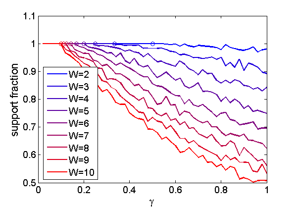
Figure 2: The fraction of distinct colors contained in the Pólya urn, which at least get sampled once within the first $N=500$ steps of the process, for numbers of colors $W=2,3,\cdots,10$ for uniformly distributed initial conditions $q_{i}=1/W$, $i=1,\cdots,W$, evaluated from $250$ runs for each $\gamma=0.01,0.02,\cdots,1$. The onset of instability $\gamma_{\rm crit}(q)=\min(q)=1/W$ (circular markers) is very well reproduced experimentally.

Since $\partial^{2}\psi_{\rm P\acute{o}lya}/\partial p_{i}^{2}<0\$if $\gamma<q_{i}$, $\psi_{\rm P\acute{o}lya}$ is maximal and case (A) applies. If $q_{i}<\gamma$, Eq (14) becomes negative but also unstable and is replaced by a boundary solution: cases (B) and (C). The Pólya max-ent not only allows us to predict $p_{i}$ from the initial prior probabilities $q_{i}$, it also identifies $\gamma$ as the crucial parameter that distinguishes between the three regimes of Pólya urn dynamics. For sufficiently large but finite $N$, the analysis above is more involved but solvable.

Assuming uniformly distributed priors, $q_{i}=1/W$ for all $i$, the max-ent result equation (14) correctly predicts uniformly distributed $\hat{p}_{i}=1/W$, while observed distributions $p$ may strongly deviate from this prediction. This result reflects the fact that despite the Pólya urn process being inherently instable (e.g. winner takes all) with little chance of predicting who in particular will win, i.e. which color of balls will dominate the others, repeating the experiment many times every color of balls has the same chance to win (or biased according to the priors $q$). This discrepancy between ensemble average and time average makes it impossible to predict who in particular will win or loose in the course of time. However, using detailed information about the process one can predict how winners win. In particular one can (i) predict the onset of instability, i.e. the emergence of colors $i$ that will effectively never be drawn, at $\gamma_{\rm crit}=\min(q)$ (compare Fig. (2)), and (ii) construct a maximum entropy functional for predicting the time dependent frequency distribution of a process, i.e. the number of times one observes states $i$ for $n$ times. As a consequence, one also can derive the rank distributions of the process, i.e. the frequency of observing balls of some color after ranking those frequencies according to their magnitude.

3.1 Rank and frequency distributions of Pólya urns

With the presented max-ent approach we now compute frequency distribution functions. Given the histogram $k=(k_{1},k_{2},\cdots k_{W})$ is obtained after $N$ iterations of the process,we define new variables,

$$n_{z}(k)=\sum_{i=1}^{W}\chi(k_{i}=z)\,,$$ (15)

where $\chi$ is the characteristic function that returns $1$ if the argument is true and $0$ if false. $n_{z}(k)$ is the number of colors $i$ that occur $z$ times after running the Pólya process for $N$ iterations. $n_{z}$ is subject to the two constraints,

$$W=\sum_{z=0}^{N}n_{z}(k)\quad{\rm and}\quad N=\sum_{z=0}^{N}n_{z}(k)z\,,$$ (16)

which can be included in the maximization procedure introducing Lagrange multipliers, $\alpha$ and $\beta$. The probability of observing some $n=(n_{1},\cdots,n_{N})$ is

$$\tilde{P}(n|\theta,N)=\sum_{\{k_{i}\geq 0|n=n(k)\}}P(k|\theta,N)\,.$$ (17)

Defining the relative frequencies $\pi_{z}=n_{z}/W$ and $\bar{p}_{z}=z/N$ we can construct the max-ent functional from $\tilde{P}(n|\theta,N)$. We identify $\tilde{\psi}(\pi|\theta,N)\equiv\log(\tilde{P}(n|\theta,N))/W$.

For the multinomial $P(k|\theta,N)={N\choose{k}}\prod_{i}q_{i}^{k_{i}}$, and uniform priors $q_{i}=1/W$ we find up to an additive constant,

$$\begin{array}[]{lcl}\tilde{\psi}(\pi|\theta,N)&=&-\sum_{z=0}^{N}\pi_{z}\log\pi_{z}\\ &&\\ &&-N\sum_{z=0}^{N}\pi_{z}\bar{p}_{z}\log\bar{p}_{z}\,.\end{array}$$ (18)

$\tilde{\psi}(\pi|\theta,N)$ has to be maximised subject to equation (16),

$$\sum_{z=0}^{N}\pi_{z}=1\quad{\rm and}\quad\sum_{z=0}^{N}\pi_{z}\bar{p}_{z}=\frac{1}{W}\,,$$ (19)

so that we get the asymptotic solution for large $W$ and large $N$, ($N\gg W\gg 1$),

$$\pi_{z}=\frac{\phi^{z}}{\zeta\ z!}\,.$$ (20)

This is the Poisson distribution, exactly as expected for multinomial processes. $\phi=Ne^{-(1+\frac{\beta}{N})}$, $\zeta$ is a normalisation constant, and $\pi_{z}$ gets maximal at $\hat{z}=\phi\sim N/W$.

For the Pólya urn with uniform priors we get from equation (17)

$$\tilde{P}(n|\theta,N)=\frac{1}{Z(\theta,N)}\frac{W!}{\prod_{z=0}^{N}n_{z}!}\prod_{z=0}^{N}\left[\frac{\left(\bar{p}_{z}+\frac{1}{N}\right)^{\frac{1}{W\gamma}}}{\bar{p}_{z}+\frac{1}{\gamma WN}}\right]^{n_{z}}\,.$$ (21)

$Z(\theta,N)$ is the normalisation. Up to a constant the max-ent functional $\tilde{\psi}_{\rm P\acute{o}lya}(\pi|\theta,N)\equiv\log(P(n|\theta,N))/W$ is

$$\begin{array}[]{lcl}\tilde{\psi}_{\rm P\acute{o}lya}(\pi|\theta,N)&=&-\sum_{z=0}^{N}\pi_{z}\log(\pi_{z})\\ &&\\ &&-\sum_{z=0}^{N}\pi_{z}\log\left(\bar{p}_{z}+\frac{1}{\gamma WN}\right)\\ &&\\ &&+\frac{1}{W\gamma}\sum_{z=0}^{N}\pi_{z}\log\left(\bar{p}_{z}+\frac{1}{N}\right)\,.\end{array}$$ (22)

maximising $\tilde{\psi}_{\rm P\acute{o}lya}(\pi|\theta,N)$ under the conditions of equation (19) provides the frequency distribution of the Pólya process for uniform priors,

$$\pi_{z}=\frac{1}{\zeta}\phi^{z}\frac{(z+1)^{\frac{1}{W\gamma}}}{z+\frac{1}{\gamma W}}\,,$$ (23)

with $\phi=\exp(-\beta)$, and normalisation $\zeta=\exp(1+\alpha)N^{\frac{1}{W\gamma}-1}$.

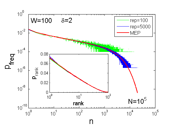
Figure 3: Frequency distribution of a Pólya urn process and uniform initial conditions (red line), for $W=100$, $\delta=2$, $a_{i}=1$ for all $i=1$, and $N=10^{5}$ steps. Simulations are shown for $100$ (green) and $5000$ (blue) repetitions of the process. Inset: Rank distributions of the max-ent result and the numerical realisations in semi-log scale.

The rank distribution of states, $f(r)$, can now be obtained as follows. $r=1$ is the state that occurs most frequently, $r=W$ is the least occupied state. For $r=1,\cdots,W$ we define intervals $[t_{r+1}t_{r}]$ with $t_{1}=N$ and $t_{W+1}=0$, such that $\sum_{t_{r+1}\leq z<t_{r}}\pi_{z}\sim 1/W$. To find $t_{i}$ we substitute sums by integrals and get

$$\frac{1}{W}=\int_{t_{r+1}}^{t_{r}}dz\ \pi_{z}\quad{\rm and}\quad f(r)=\frac{W}{N}\int_{t_{r+1}}^{t_{r}}dz\ \pi_{z}z\,.$$ (24)

Results for the frequency distributions for $a_{i}=1$, $W=100$, and $\delta=2$ are shown in Fig. (3), together with a numerical simulation for the same process. The inset shows the rank distribution. The Pólya max-ent predicts frequency and rank distribution extremely well.

The above results were all derived under the assumption that $\gamma>0$ is sufficiently large. By numerical simulation we find that the solution equation (23) also works remarkably well for very small values of $\gamma$, if the value of $\gamma$ in equation (23) is appropriately renormalised, $\gamma\to\gamma_{0}$. In particular for $\gamma=0$ (multinomial process) we sample the Poisson distribution function, equation (20). The Pólya max-ent solution recovers the Poisson distribution extremely well if $\gamma=0\to\gamma_{0}(W,N)=1/(N+3W)$. In this sense the Pólya max-ent remains adequate in the limit of small $\gamma$.

4 Discussion

Pólya urns offer a transparent way to study self-reinforcing systems with explicit path-dependence. Based on the microscopic rules of the process, we constructively derive the generalised information divergence $\psi$ which acts as the corresponding non-multinomial max-ent functional. This provides us with an alternative to the ensemble approach for path-dependent processes that is able to predict the statistics of the system. The maximisation of the functional leads to an equivalent to the classical maximum configuration approach, which by definition predicts the most likely distribution function. In this sense maximum configuration predictions are optimal, and can be used to understand even details of the statistics of path-dependent processes, such as their frequency and rank distributions.

It is interesting to note that the functional playing the role of the entropy in the Pólya processes violates at least two of the four classic information theoretic (Shannon-Khinchin) axioms which determine Shannon entropy [8]. Even more, for the finite size Pólya entropy, three of the four axioms are violated. This indicates that the classes of generalised entropy functionals that are useful for a max-ent approach may be even larger than expected [30, 31]. One might speculate that in this sense the classic information theoretic axioms are too rigorous, when it comes to characterising information flow and phase space structure in non-stationary, path-dependent, processes. The observation that each particular class of non-multinomial processes requires a matching max-ent functional that can in principle be constructed from the generative rules of a process, opens the applicability of max-ent approaches for a wide range of complex systems in a meaningful way. The generalized max-ent approach in this sense responds to Einsteins comment on Boltzmann’s principle in a natural way.

Finally we note the implications for statistical inference with data from non-multinomial sources, which implicitly involves the estimation of the parameters $\theta$ that determine the process that generates the data. In a max-ent approach this is done by fitting classes of curves to the data, that are consistent with the max-ent approach. For doing this, the nature of the process, i.e. its class, needs to be known. For path-dependent processes, which are non-multinomial by nature, entropy will no longer be Shannon entropy $H$, and the information divergence will no longer be the Kullback-Leibler divergence.

References

- [1] Einstein A 1910, Theorie der Opaleszenz von homogenen Flüssigkeiten und Flüssigkeitsgemischen in der Nähe des kritischen Zustandes. Ann. d. Phys. 33, 1275.
- [2] Landau L D and Lifshitz E M 1980, Statistical Physics, Course in Theoretical Physics 5, footnote p. 12. (Elsevier, 3’rd edition)
- [3] Peters O. 2011, The time resolution of the St Petersburg paradox. Phil. Trans. R. Soc. A 396, 4913-4931
- [4] Hanel R, Thurner S, and Gell-Mann M 2014, How multiplicity of random processes determines entropy: derivation of the maximum entropy principle for complex systems, Proc. Nat. Acad. Sci. USA 111 6905–6910.
- [5] Shannon C E 1948, A Mathematical Theory of Communication, Bell Syst. Tech. J. 27 379 -423, 623 -656.
- [6] Jaynes E T 1968, Prior Probabilities, IEEE Trans Sys Sci and Cybernetics 4 227- 241.
- [7] Kullback S, and Leibler R A 1951, On information and sufficiency, Ann. Math. Stat. 22 79- 86.
- [8] Khinchin A I 1957, Mathematical foundations of information theory, (Dover Publ., New York).
- [9] Eggenberger F, G. Pólya G 1923, Über die Statistik verketteter Vorgänge, Z. Angew. Math. Mech. 1 279–289.
- [10] Pólya G 1930, Sur quelques points de la théorie des probabilités, Ann. Inst. Henri Poincare 1 117–161.
- [11] Wallstrom T C 2012, The equalization probability of Pólya urn, Am. Math. Mon. 119 516–518.
- [12] Johnson N L and Kotz S 1977, Urn Models and Their Application: An Approach to Modern Discrete Probability Theory, In Urn models and their application. An approach to modern discrete probability theory. (John Wiley, New York).
- [13] Mahmoud H 2008, Pólya Urn Models, Texts in Statistical Science, (Chapman & Hall/CRC Texts in Statistical Science, Taylor and Francis Ltd, Hoboken, NJ).
- [14] Kotz S, Mahmoud H, and Robert P 2000, On generalised Pólya urn models, Stat. Prob. Lett. 49 163–173.
- [15] Janson S 2004, Functional limit theorems for multitype branching processes and generalised Pólya urns, Stoch. Proc. Appl. 110 177 -245.
- [16] Smythe R T 1996, Central limit theorems for urn models, Stoch. Proc. Appl. 65 115–137.
- [17] Gouet R 1993, Martingale Functional Central Limit Theorems for a generalised Pólya Urn, Ann. Prob. 21 1624–1639.
- [18] Tolusso D and Wang X 2011, Interval estimation for response adaptive clinical trials, Comput. Stat. Data Anal. 55 725–730.
- [19] Binder B J and Landman K A 2009, Tissue growth and the Pólya distribution, Aust. J. Eng. Edu. 15 35–42.
- [20] Crouch C and Farrell H 2004, Breaking the Path of Institutional Development? Alternatives to the New Determinism, Ratio. Soc. 16 5–43.
- [21] Bagchi A and Pal A K 1985, Asymptotic Normality in the generalised Pólya Eggenberger Urn Model, with an Application to Computer Data Structures, SIAM J. Algeb. Disc. Meth. 6 394 -405.
- [22] Geppert T 2012, EU-Agrar- und Regionalpolitik, Wie vergangene Entscheidungen zukünftige Entwicklungen beeinflussen - Pfadabhängigkeit und die Reformfähigkeit von Politikfeldern, PhD Thesis, (University of Bamberg Press, Bamberg).
- [23] Donnelly P 1986, Partition structures, Pólya urns, the Ewens sampling formula, and the ages of alleles, Theor. Popul. Biol. 30 271- 288.
- [24] Hoppe F M 1984, Pólya-like urns and the Ewens’ sampling formula, J. Math. Biol. 20 91–94.
- [25] Banerjee A, Burlina P, and Alajaji F 1999, Image segmentation and labeling using the Pólya urn model, IEEE Trans. Image. Proc. 8 1243–1253.
- [26] Alexander J M, Skyrms B, and Zabell S 2012, Inventing new signals, Dyn. Games Appl. 2 129–145.
- [27] Tria F, Loreto V,Servedio V D P, and Strogatz S H 2014, The dynamics of correlated novelties, Sci. Rep. 4:5890.
- [28] Grendar M, and Niven R K 2010, The Pólya information divergence, Info. Sci. 180 4189- 4194.
- [29] Sanov I N 1957, On the probability of large deviations of random variables, Mat. Sbornik 42 11–44.
- [30] Hanel R and Thurner S 2011, A comprehensive classification of complex statistical systems and an ab initio derivation of their entropy and distribution function, EPL 93:20006.
- [31] Hanel R and Thurner S 2011, When do generalised entropies apply? How phase space volume determines entropy, EPL 96:50003.