I/O Efficient Core Graph Decomposition at
Web Scale

Abstract

Core decomposition is a fundamental graph problem with a large number of applications. Most existing approaches for core decomposition assume that the graph is kept in memory of a machine. Nevertheless, many real-world graphs are big and may not reside in memory. In the literature, there is only one work for I/O efficient core decomposition that avoids loading the whole graph in memory. However, this approach is not scalable to handle big graphs because it cannot bound the memory size and may load most parts of the graph in memory. In addition, this approach can hardly handle graph updates. In this paper, we study I/O efficient core decomposition following a semi-external model, which only allows node information to be loaded in memory. This model works well in many web-scale graphs. We propose a semi-external algorithm and two optimized algorithms for I/O efficient core decomposition using very simple structures and data access model. To handle dynamic graph updates, we show that our algorithm can be naturally extended to handle edge deletion. We also propose an I/O efficient core maintenance algorithm to handle edge insertion, and an improved algorithm to further reduce I/O and CPU cost by investigating some new graph properties. We conduct extensive experiments on $12$ real large graphs. Our optimal algorithm significantly outperform the existing I/O efficient algorithm in terms of both processing time and memory consumption. In many memory-resident graphs, our algorithms for both core decomposition and maintenance can even outperform the in-memory algorithm due to the simple structures and data access model used. Our algorithms are very scalable to handle web-scale graphs. As an example, we are the first to handle a web graph with $978.5$ million nodes and $42.6$ billion edges using less than $4.2$ GB memory.

I Introduction

Graphs have been widely used to represent the relationships of entities in a large spectrum of applications such as social networks, web search, collaboration networks, and biology. With the proliferation of graph applications, research efforts have been devoted to many fundamental problems in managing and analyzing graph data. Among them, the problem of computing the $k$-core of a graph has been recently studied [11, 27, 19, 12]. Here, given a graph $G$, the $k$-core of $G$ is the largest subgraph of $G$ such that all the nodes in the subgraph have a degree of at least $k$ [28]. For each node $v$ in $G$, the core number of $v$ denotes the largest $k$ such that $v$ is contained in a $k$-core. The core decomposition problem computes the core numbers for all nodes in $G$. Given the core decomposition of a graph $G$, the $k$-core of $G$ for all possible $k$ values can be easily obtained. There is a linear time in-memory algorithm, devised by Batagelj and Zaversnik [9], to compute core numbers of all nodes.

Applications. Core decomposition is widely adopted in many real-world applications, such as community detection [15, 12], network clustering [30], network topology analysis [28, 5], network visualization [4, 3], protein-protein network analysis [2, 7], and system structure analysis [31]. In addition, many researches are devoted on the core decomposition for specific kinds of networks [13, 21, 25, 22, 17, 10]. Moreover, due to the elegant structural property of a $k$-core and the linear solution for core decomposition, a large number of graph problems use core decomposition as a subroutine or a preprocessing step, such as clique finding [8], dense subgraph discovery [6, 26], approximation of betweeness scores [16], and some variants of community search problems [29, 18].

Motivation. Despite the large amount of applications for core decomposition in various networks, most of the solutions for core decomposition assume that the graph is resident in the main memory of a machine. Nevertheless, many real-world graphs are big and may not reside entirely in the main memory. For example, the $\mathsf{Facebook}$ social network contains $1.32$ billion nodes and $140$ billion edges; and a sub-domain of the web graph $\mathsf{Clueweb}$ contains $978.5$ million nodes and $42.6$ billion edges. In the literature, the only solution to study I/O efficient core decomposition is $\mathsf{EMCore}$ proposed by Cheng et al. [11], which allows the graph to be partially loaded in the main memory. $\mathsf{EMCore}$ adopts a graph partition based approach and partitions are loaded into main memory whenever necessary. However, $\mathsf{EMCore}$ cannot bound the size of the memory and to process many real-world graphs, $\mathsf{EMCore}$ still loads most edges of the graph in the main memory. This makes $\mathsf{EMCore}$ unscalable to handle web-scale graphs. In addition, many real-world graphs are usually dynamically updating. The complex structure used in $\mathsf{EMCore}$ makes it very difficult to handle graph updates incrementally.

Our Solution. In this paper, we address the drawbacks of the existing solutions for core decomposition and propose new algorithms for core decomposition with guaranteed memory bound. Specifically, we adopt a semi-external model. It assumes that the nodes of the graph, each of which is associated with a small constant amount of information, can be loaded in main memory while the edges are stored on disk. We find that this assumption is practical in a large number of real-world web-scale graphs, and widely adopted to handle other graph problems [32, 33, 20]. Based on such an assumption, we are able to handle core decomposition I/O efficiently using very simple structures and data access mechanism. These enable our algorithm to efficiently handle graph updates incrementally under the semi-external model.

Contributions. We make the following contributions:

(1) The first I/O efficient core decomposition algorithm with memory guarantee. We propose an I/O efficient core decomposition algorithm following the semi-external model. Our algorithm only keeps the core numbers of nodes in memory and updates the core numbers iteratively until convergency. In each iteration, we only require sequential scans of edges on disk. To the best of our knowledge, this is the first work for I/O efficient core decomposition with memory guarantee.

(2) Several optimization strategies to largely reduce the I/O and CPU cost. Through further analysis, we observe that when the number of iterations increases, only a very small proportion of nodes have their core numbers updated in each iteration, and thus a total scan of all edges on disk in each iteration will result in a large number of waste I/O and CPU cost. Therefore, we propose optimization strategies to reduce these cost. Our first strategy is based on the observation that the update of core number for a node should be triggered by the update of core number for at least one of its neighbors in the graph. Our second strategy further maintains more node information. As a result, we can completely avoid waste I/Os and core number computations, in the sense that each I/O is used in a core number computation that is guaranteed to update the core number of the corresponding node. Both optimization strategies can be easily adapted in our algorithm framework.

(3) The first I/O efficient core decomposition algorithm to handle graph updates. We consider dynamical graphs with edge deletion and insertion. Our semi-external algorithm can naturally support edge deletion with a simple algorithm modification. For edge insertion, we first utilize some graph properties adopted in existing in-memory algorithms [27, 19] to handle graph updates for core decomposition. We propose a two-phase semi-external algorithm to handle edge insertion using these graph properties. We further explore some new graph properties, and propose a new one-phase semi-external algorithm to largely reduce the I/O and CPU cost for edge insertion. To the best of our knowledge, this is the first work for I/O efficient core maintenance on dynamic graphs.

(4) Extensive performance studies. We conduct extensive performance studies using $12$ real graphs with various graph properties to demonstrate the efficiency of our algorithms. We compare our algorithm, for memory-resident graphs, with $\mathsf{EMCore}$ [11] and the in-memory algorithm [9]. Both our core decomposition and core maintenance algorithms are much faster and use much less memory than $\mathsf{EMCore}$. In many datasets, our algorithms for core decomposition and maintenance are even faster than the in-memory algorithm due to the simple structure and data access model used. Our algorithms are very scalable to handle web-scale graphs. For instance, we consume less than $4.2$ GB memory to handle the web-graph $\mathsf{Clueweb}$ with $978.5$ million nodes and $42.6$ billion edges.

Outline. Section II provides the preliminaries and problem statement. Section III introduces some existing solutions for core decomposition under different settings. Section IV presents our semi-external core decomposition algorithm and explores some optimization strategies to reduce I/O and CPU cost. Section V discusses how to design semi-external algorithms to maintain core numbers incrementally when the graph is dynamically updated, and investigates some new graph properties to improve the algorithm when handling edge insertion. Section VI evaluates all the introduced algorithms using extensive experiments. Section VII reviews the related work and Section VIII concludes the paper.

II Problem Statement

Consider an undirected and unweighted graph $G=(V,E)$, where $V(G)$ represents the set of nodes and $E(G)$ represents the set of edges in $G$. We denote the number of nodes and the number of edges of $G$ by $n$ and $m$ respectively. We use ${\mathsf{nbr}}(u,G)$ to denote the set of neighbors of $u$ for each node $u\in V(G)$, i.e., ${\mathsf{nbr}}(u,G)=\{v|(u,v)\in E(G)\}$. The degree of a node $u\in V(G)$, denoted by ${\mathsf{deg}}(u,G)$, is the number of neighbors of $u$ in $G$, i.e., ${\mathsf{deg}}(u,G)=|{\mathsf{nbr}}(u,G)|$. For simplicity, we use ${\mathsf{nbr}}(u)$ and ${\mathsf{deg}}(u)$ to denote ${\mathsf{nbr}}(u,G)$ and ${\mathsf{deg}}(u,G)$ respectively if the context is self-evident. A graph $G^{\prime}$ is a subgraph of $G$, denoted by $G^{\prime}\subseteq G$, if $V(G^{\prime})\subseteq V(G)$ and $E(G^{\prime})\subseteq E(G)$. Given a set of nodes $V_{c}\subseteq V$, the induced subgraph of $V_{c}$, denoted by $G(V_{c})$, is a subgraph of $G$ such that $G(V_{c})=(V_{c},\{(u,v)\in E(G)|u,v\in V_{c}\})$.

Definition 2.1: ($k$-Core) Given a graph $G$ and an integer $k$, the $k$-core of graph $G$, denoted by $G_{k}$, is a maximal subgraph of $G$ in which every node has a degree of at least $k$, i.e., $\forall v\in V(G_{k}),d(v,G_{k})\geq k$ [28]. $\Box$

Let $k_{max}$ be the maximum possible $k$ value such that a $k$-core of $G$ exists. According to [9], the $k$-cores of graph $G$ for all $1\leq k\leq k_{max}$ have the following property:

Property 2.1: $\forall 1\leq k<k_{max}:G_{k+1}\subseteq G_{k}$. $\Box$

Next, we define the core number for each $v\in V(G)$.

Definition 2.2: (Core Number) Given a graph $G$, for each node $v\in V(G)$, the core number of $v$, denoted by ${\mathsf{core}}(v,G)$, is the largest $k$, such that $v$ is contained in a $k$-core, i.e., ${\mathsf{core}}(v,G)=\max\{k|v\in V(G_{k})\}$. For simplicity, we use ${\mathsf{core}}(v)$ to denote ${\mathsf{core}}(v,G)$ if the context is self-evident. $\Box$

Based on Property II and Definiton II, we can easily derive the following lemma:

Lemma 2.1: Given a graph $G$ and an integer $k$, let $V_{k}=\{v\in V(G)|{\mathsf{core}}(v)\geq k\}$, we have $G_{k}=G(V_{k})$. $\Box$

Problem Statement. In this paper, we study the problem of Core Graph Decomposition (or Core Decomposition for short), which is defined as follows: Given a graph $G$, core decomposition computes the the $k$-cores of $G$ for all $1\leq k\leq k_{max}$. We also consider how to update the $k$-cores for of $G$ for all $1\leq k\leq k_{max}$ incrementally when $G$ is dynamically updated by insertion and deletion of edges.

According to Lemma II, core decomposition is equivalent to computing ${\mathsf{core}}(v)$ for all $v\in V(G)$. Therefore, in this paper, we study how to compute ${\mathsf{core}}(v)$ for all $v\in V(G)$ and how to maintain them incrementally when graph is dynamically updating .

Considering that many real-world graphs are huge and cannot entirely reside in main memory, we aim to design I/O efficient algorithms to compute and maintain the core numbers of all nodes in the graph $G$. To analyze the algorithm, we use the external memory model introduced in [1]. Let $M$ be the size of main memory and let $B$ be the disk block size. A read I/O will load one block of size $B$ from disk into main memory, and a write I/O will write one block of size $B$ from the main memory into disk.

Assumption. In this paper, we follow a semi-external model by assuming that the nodes can be loaded in main memory while the edges are stored on disk, i.e., we assume that $M\geq c\times|V(G)|$ where $c$ is a small constant. This assumption is practical because in most social networks and web graphs, the number of edges is much larger than the number of nodes. For example, in SNAP, among $79$ real-world graphs, the largest graph contains $65$ M nodes and $1.8$ G edges. In KONET, among $239$ real-world graphs, the largest graph contains $68$ M nodes and $2.6$ G edges. In WebGraph, among $75$ real-world graphs, the largest graph contains $721$ M nodes and $137.3$ G edges, and the second largest graph contains $978$ M nodes and $42.6$ G edges. In our proposed algorithm of this paper, when handling the two largest graphs in WebGraph, we only require $3.1$ GB and $4.2$ GB memory respectively, which is affordable even by a normal PC.

Graph Storage. In this paper, we use an edge table on disk to store the edges of $G$. e.g., we store ${\mathsf{nbr}}(v_{1})$, ${\mathsf{nbr}}(v_{2})$, $\ldots$, ${\mathsf{nbr}}(v_{n})$ consecutively as adjacency lists in the edge table. We also use a node table on disk to store the offsets and degrees for $v_{1}$, $v_{2}$, $\ldots$, $v_{n}$ consecutively. To load the neighbors of a certain node $v_{i}\in V(G)$, we can access the node table to get the offset and ${\mathsf{deg}}(v_{i})$ for $v_{i}$, and then access the edge table to load ${\mathsf{nbr}}(v_{i})$.

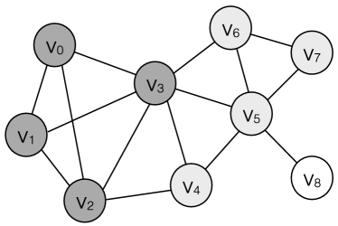
Figure 1: A Sample Graph $G$ and its Core Decomposition

Example 2.1: Consider a graph $G$ in Fig. 1, the induced subgraph of $\{v_{0},$ $v_{1},$ $v_{2},$ $v_{3}\}$ is a $3\text{-}core$ in which every node has a degree at least $3$. Since no $4$-core exists in $G$, we have ${\mathsf{core}}(v_{0})={\mathsf{core}}(v_{1})={\mathsf{core}}(v_{2})={\mathsf{core}}(v_{3})=3$. Similarly, we can derive that ${\mathsf{core}}(v_{4})={\mathsf{core}}(v_{5})={\mathsf{core}}(v_{6})={\mathsf{core}}(v_{7})=2$ and ${\mathsf{core}}(v_{8})=1$. When an edge $(v_{7},v_{8})$ is inserted in $G$, ${\mathsf{core}}(v_{8})$ increases from $1$ to $2$, and the core numbers of other nodes keep unchanged. $\Box$

III Existing Solutions

In this section, we introduce three state-of-the-art existing solutions for core decomposition in different settings, namely, in-memory core decomposition, I/O efficient core decomposition, and in-memory core maintenance.

In-memory Core Decomposition. The state-of-the-art in-memory core decomposition algorithm, denote by ${\mathsf{IMCore}}$, is proposed in [9]. The pseudocode of ${\mathsf{IMCore}}$ is shown in Algorithm 1. The algorithm processes the node with core number $k$ in increasing order of $k$. Each time, $k$ is selected as the minimum degree of current nodes in the graph (line 3). Whenever there exists a node $v$ with degree no larger than $k$ in the graph (line 4), we can guarantee that the core number of $v$ is $k$ (line 5) and we remove $v$ with all its incident edges from the graph (line 6). Finally, the core number of all nodes are returned (line 7). With the help of bin sort to maintain the minimum degree of the graph, ${\mathsf{IMCore}}$ can achieve a time complexity of $O(m+n)$, which is optimal.

Algorithm 1 ${\mathsf{IMCore}}($Graph $G)$

1:  $G^{\prime}\leftarrow G$;

2:  while $G^{\prime}\neq\emptyset$ do

3:     $k\leftarrow\min_{v\in V(G^{\prime})}{\mathsf{deg}}(v,G^{\prime})$;

4:     while $\exists v\in V(G^{\prime}):{\mathsf{deg}}(v,G^{\prime})\leq k$ do

5:        ${\mathsf{core}}(v)\leftarrow k$;

6:        remove $v$ and its incident edges from $G^{\prime}$;

7:  return ${\mathsf{core}}(v)$ for all $v\in V(G)$;

I/O Efficient Core Decomposition. The state-of-the-art efficient core decomposition algorithm is proposed in [11]. The algorithm, denoted as ${\mathsf{EMCore}}$, is shown in Algorithm 2. It first divides the whole graph $G$ into partitions on disk (line 1). Each partition contains a disjoint set of nodes along with their incident edges. An upper bound of ${\mathsf{core}}(v)$, denoted by ${{\mathsf{ub}}}(v)$, is computed for each node $v$ in each partition $P_{i}$. Then the algorithm iteratively computes the core numbers for nodes in a top-down manner.

In iteration, the nodes with core values falling in a certain range $[k_{l},k_{u}]$ is computed (line 6-14). Here, $k_{l}$ is estimated based on the number of partitions that can be loaded in main memory (line 6). In line 7, the algorithm computes the set of partitions each of which contains at leat one node $v$ with ${{\mathsf{ub}}}(v)$ falling in $[k_{l},k_{u}]$, and in line 8, all such partitions are loaded in main memory to form an in-memory graph $G_{mem}$. In line 9, an in-memory core decomposition algorithm is applied on $G_{mem}$, and those nodes in $G_{mem}$ with core numbers falling in $[k_{l},k_{u}]$ get their exact core numbers in $G$. After that, for all partitions loaded in memory (line 10), those nodes with exact core numbers computed are removed from the partition (line 11), and the their core number upper bounds and degrees are updated accordingly (line 12). Here the new node degrees have to consider the deposited degrees from the removed nodes. Finally, the in-memory partitions are merged and written back to disk (line 13), and $k_{u}$ is set to be $k_{l}-1$ to process the next range of $k$ values in the next iteration.

The I/O complexity of ${\mathsf{EMCore}}$ is $O(\frac{k_{max}\cdot(m+n)}{B})$. The CPU complexity of ${\mathsf{EMCore}}$ is $O(k_{max}\cdot(m+n))$. However, the space complexity of ${\mathsf{EMCore}}$ cannot be well bounded. In the worst case, it still requires $O(m+n)$ memory space to load the whole graph into main memory. Therefore, ${\mathsf{EMCore}}$ is not scalable to handle large-sized graphs.

Algorithm 2 ${\mathsf{EMCore}}($Graph $G$ on Disk$)$

1:  divide $G$ into partitions ${\cal P}=\{P_{1},P_{2},\ldots,P_{t}\}$ on disk;

2:  for all partition $P_{i}\in{\cal P}$ do

3:     compute ${{\mathsf{ub}}}(v)$ for all $v\in V(P_{i})$;

4:  $k_{u}\leftarrow+\infty$;

5:  while $k_{u}>0$ do

6:     estimate $k_{l}$;

7:     ${\cal P}_{mem}\leftarrow\{P_{i}\in{\cal P}|\exists v\in V(P_{i}):{{\mathsf{ub}}}(v)\in[k_{l},k_{u}]\}$;

8:     $G_{mem}\leftarrow$ load partitions in ${\cal P}_{mem}$ in main memory;

9:     ${\mathsf{core}}(v)\leftarrow{\mathsf{core}}(v,G_{mem})$ for all ${\mathsf{core}}(v,G_{mem})\in[k_{l},k_{u}]$;

10:     for all partition $P_{i}\in{\cal P}_{mem}$  do

11:        remove nodes $v$ with ${\mathsf{core}}(v,G_{mem})\in[k_{l},k_{u}]$ from $P_{i}$;

12:        update ${{\mathsf{ub}}}(v)$ and ${\mathsf{deg}}(v)$ for all $v\in V(P_{i})$;

13:        write $P_{i}$ back to disk (merge small partitions if necessary);

14:     $k_{u}\leftarrow k_{l}-1$;

15:  return ${\mathsf{core}}(v)$ for all $v\in V(G)$;

In-memory Core Maintenance. To handle the case when the graph is dynamically updated by insertion and deletion of edges, the state-of-the-art core maintenance algorithms are proposed in [27] and [19], which are based on the same findings shown in the following theorems:

Theorem 3.1: If an edge is inserted into (deleted from) graph $G$, the core number ${\mathsf{core}}(v)$ for any $v\in V(G)$ may increase (decrease) by at most $1$. $\Box$

Theorem 3.2: If an edge $(u,v)$ is inserted into (deleted from) graph $G$, suppose ${\mathsf{core}}(v)\leq{\mathsf{core}}(u)$ and let $V^{\prime}$ be the set of nodes whose core numbers have changed, if $V^{\prime}\neq\emptyset$, we have:
$\bullet$ $G(V^{\prime})$ is a connected subgraph of $G$;
$\bullet$ $v\in V^{\prime}$; and
$\bullet$ $\forall v^{\prime}\in V^{\prime}:{\mathsf{core}}(v^{\prime})={\mathsf{core}}(v)$; $\Box$

Based on Theorem 2 and Theorem 2, after an edge $(u,v)$ is inserted into (deleted from) graph $G$, suppose ${\mathsf{core}}(v)\leq{\mathsf{core}}(u)$, instead of computing the core numbers for all nodes in $G$ from scratch, we can restraint the core computation within a small range of nodes $V^{\prime}$ in $G$. Specifically, we can follow a two-step approach: In the first step, we can perform a depth-first-search from node $v$ in $G$ to compute all nodes $v^{\prime}$ with ${\mathsf{core}}(v^{\prime})={\mathsf{core}}(v)$ and are reachable from $v$ via a path that consists of nodes with core numbers equal to ${\mathsf{core}}(v)$. Such nodes form a set $V^{\prime}$ which is usually much smaller than $V(G)$. In the second step, we only restraint the core number updates within the subgraph $G(V^{\prime})$ in memory, and each update increases (decreases) the core number of a node by at most $1$. The algorithm details and other optimization techniques can be found in [27] and [19].

IV I/O Efficient Core Decomposition

In this section, we present our basic semi-external algorithm and then discuss how to improve the algorithm by partial node computation. Finally, we will propose an algorithm by eliminating all useless node computations.

IV-A Basic Semi-external Algorithm

Drawback of $\mathsf{EMCore}$. $\mathsf{EMCore}$ (Algorithm 2) is the state-of-the-art I/O efficient core decomposition algorithm. However, $\mathsf{EMCore}$ cannot be used to handle big graphs, since the number of partitions to be loaded into main memory in each iteration cannot be well-bounded. In line 7-8 of Algorithm 2, as long as a partition contains a node $v$ with ${{\mathsf{ub}}}(v)\in[k_{l},k_{u}]$, the whole partition needs to be loaded into main memory. When $k_{u}$ becomes small, it is highly possible for a partition to contain a node $v$ with ${{\mathsf{ub}}}(v)\in[k_{l},k_{u}]$. Consequently, almost all partitions are loaded into main memory. Due to this reason, the space used for $\mathsf{EMCore}$ is $O(m+n)$, and it cannot be significantly reduced in practice, as verified in our experiments.

Locality Property. In this paper, we aim to design a semi-external algorithm for core decomposition. First, we introduce a locality property for core numbers, which is proposed in [23], as shown in the following theorem:

Theorem 4.1: (Locality) Given a graph $G$, the ${\mathsf{core}}(v)$ values for all $v\in V(G)$ are their core numbers in $G$ iff:

$\bullet$ There exists $V_{k}\subseteq{\mathsf{nbr}}(v)$ such that: $|V_{k}|={\mathsf{core}}(v)$ and $\forall u\in V_{k},{\mathsf{core}}(u)\geq{\mathsf{core}}(v)$; and

$\bullet$ There does not exists $V_{k+1}\subseteq{\mathsf{nbr}}(v)$ such that: $|V_{k+1}|={\mathsf{core}}(v)+1$ and $\forall u\in V_{k+1},{\mathsf{core}}(u)\geq{\mathsf{core}}(v)+1$. $\Box$

Based on Theorem IV-A, the core number ${\mathsf{core}}(v)$ for a node $v\in V(G)$ can be calculated using the following recursive equation:

$${\mathsf{core}}(v)=\text{max}\ k\ \text{s.t.}\ |\{u\in{\mathsf{nbr}}(v)|{\mathsf{core}}(u)\geq k\}|\geq k$$ (1)

Based on the locality property of core numbers, a distributed algorithm is designed in [23]. In which each node $v$ initially assigns its core number as an arbitrary core number upper bound (e.g., $\deg(v)$), and keeps updating its core numbers using Eq. 1 until convergence.

Algorithm 3 ${\mathsf{SemiCore}}($Graph $G$ on Disk$)$

1:  $\overline{{\mathsf{core}}}(v)\leftarrow{\mathsf{deg}}(v)$ for all $v\in V(G)$;

2:  ${\mathsf{update}}\leftarrow\textbf{true}$;

3:  while ${\mathsf{update}}$ do

4:     ${\mathsf{update}}\leftarrow\textbf{false}$;

5:     for $v\leftarrow v_{1}$ to $v_{n}$ do

6:        load ${\mathsf{nbr}}(v)$ from disk;

7:        ${\mathsf{c}}_{{\mathsf{old}}}\leftarrow\overline{{\mathsf{core}}}(v)$;

8:        $\overline{{\mathsf{core}}}(v)\leftarrow{\mathsf{LocalCore}}({\mathsf{c}}_{{\mathsf{old}}},{\mathsf{nbr}}(v))$;

9:        if $\overline{{\mathsf{core}}}(v)\neq{\mathsf{c}}_{{\mathsf{old}}}$ then ${\mathsf{update}}\leftarrow\textbf{true}$;

10:  return $\overline{{\mathsf{core}}}(v)$ for all $v\in V(G)$;

11:  Procedure ${\mathsf{LocalCore}}({\mathsf{c}}_{{\mathsf{old}}}$, ${\mathsf{nbr}}(v))$

12:  ${\mathsf{num}}(i)\leftarrow 0$ for all $1\leq i\leq c$;

13:  for all $u\in{\mathsf{nbr}}(v)$ do

14:     $i\leftarrow\min\{{\mathsf{c}}_{{\mathsf{old}}},\overline{{\mathsf{core}}}(u)\}$;

15:     ${\mathsf{num}}(i)\leftarrow{\mathsf{num}}(i)+1$;

16:  $s\leftarrow 0$;

17:  for $k\leftarrow{\mathsf{c}}_{{\mathsf{old}}}$ to $1$ do

18:     $s\leftarrow s+{\mathsf{num}}(k)$;

19:     if $s\geq i$ then break;

20:  return $k$;

Basic Solution. In this paper, we make use of the locality property to design a semi-external algorithm for core decomposition. The pseudocode of our basic algorithm is shown in Algorithm 3. Here, we use $\overline{{\mathsf{core}}}(v)$ to denote the intermediate core number for $v$, which is always an upper bound of ${\mathsf{core}}(v)$ and will finally converge to ${\mathsf{core}}(v)$. Initially, $\overline{{\mathsf{core}}}(v)$ is assigned as an arbitrary upper bound of ${\mathsf{core}}(v)$ (e.g., $\deg(v)$). Then, we iteratively update $\overline{{\mathsf{core}}}(v)$ for all $v\in V(G)$ using the locality property until convergence (line 2-9).

In each iteration (line 5-9), we sequentially scan the node table on disk to get the offset and ${\mathsf{deg}}(v)$ for each node $v$ from $v_{1}$ to $v_{n}$ (line 5). Then we load ${\mathsf{nbr}}(v)$ from disk using the offset and ${\mathsf{deg}}(v)$ for each such node $v$, (line 6). Recall that the edge table on disk stores ${\mathsf{nbr}}(v)$ from $v_{1}$ to $v_{n}$ sequentially. Therefore, we can load ${\mathsf{nbr}}(v)$ easily using sequential scan of the edge table on disk. In line 7-9, we record the original core number ${\mathsf{c}}_{{\mathsf{old}}}$ of $v$ (line 7); compute an updated core number of $v$ using Eq. 1 by invoking ${\mathsf{LocalCore}}({\mathsf{c}}_{{\mathsf{old}}},{\mathsf{nbr}}(v))$(line 8); and continue the iteration if $\overline{{\mathsf{core}}}(v)$ is updated (line 9). Finally, when $\overline{{\mathsf{core}}}(v)$ for all $v\in V(G)$ keeps unchanged, we return them as their core numbers (line 10).

The procedure ${\mathsf{LocalCore}}({\mathsf{c}}_{{\mathsf{old}}},{\mathsf{nbr}}(v))$ to compute the new core number of $v$ using Eq. 1 is shown in line 11-20 of Algorithm 3. We use ${\mathsf{num}}(i)$ to denote the number of neighbors of $v$ with $\overline{{\mathsf{core}}}$ equals $i$ (if $i<{\mathsf{c}}_{{\mathsf{old}}}$) or with $\overline{{\mathsf{core}}}$ no smaller than $i$ (if $i={\mathsf{c}}_{{\mathsf{old}}}$) (line 12-15). After computing ${\mathsf{num}}(i)$ for all $1\leq i\leq{\mathsf{c}}_{{\mathsf{old}}}$, we decrease $k$ from ${\mathsf{c}}_{{\mathsf{old}}}$ to $1$ (line 17), and for each $k$, we compute the number of neighbors of $v$ with $\overline{{\mathsf{core}}}\geq k$, denotes as $s$ (line 18), i.e., $s=|\{u\in{\mathsf{nbr}}(v)|{\mathsf{core}}(u)\geq k\}|$. Once $s\geq k$, we get the maximum $k$ with $|\{u\in{\mathsf{nbr}}(v)|{\mathsf{core}}(u)\geq k\}|\geq k$, and we return $k$ as the new core number (line 20). Since ${\mathsf{c}}_{{\mathsf{old}}}\leq{\mathsf{nbr}}(v)$, the time complexity of ${\mathsf{LocalCore}}({\mathsf{c}}_{{\mathsf{old}}},{\mathsf{nbr}}(v))$ is $O({\mathsf{deg}}(v))$.

Algorithm Analysis. The space, CPU time, I/O complexities of Algorithm 3 is shown in the following theorem:

Theorem 4.2: Algorithm 3 requires $O(n)$ memory. Let $l$ be the number of iterations of Algorithm 3, the I/O complexity of Algorithm 3 is $O(\frac{l\cdot(m+n)}{B})$, and the CPU time complexity of Algorithm 3 is $O(l\cdot(m+n))$. $\Box$

Proof: First, three in-memory arrays are used in Algorithm 3, $\overline{{\mathsf{core}}}$, ${\mathsf{num}}$, and ${\mathsf{nbr}}$, all of which can be bounded using $O(n)$ memory. Consequently, Algorithm 3 requires $O(n)$ memory. Second, in each iteration, Algorithm 3 scans the node table and edge table sequentially once. Therefore, Algorithm 3 consumes $O(\frac{l\cdot(m+n)}{B})$ I/Os. Finally, in each iteration, for each node $v$, we invoke ${\mathsf{LocalCore}}({\mathsf{c}}_{{\mathsf{old}}},{\mathsf{nbr}}(v))$ which requires $O({\mathsf{deg}}(v))$ CPU time. As a result, the CPU time complexity for Algorithm 3 is $O(l\cdot(m+n))$. $\Box$

Discussion. Note that we use a value $l$ to denote the number of iterations of Algorithm 3. Although $l$ is bounded by $n$ as proved in [23], it is much smaller in practice and is usually not largely influenced by the size of the graph. For example, in a social network $\mathsf{Twitter}$ with $n=41.7$ M, $m=1.47$ G, and $k_{max}=2488$ used in our experiments, the number of iterations using Algorithm 3 is only $62$. In a web graph $\mathsf{UK}$ with $n=105.9$ M, $m=3.74$ G, and $k_{max}=5704$ used in our experiments, the number of iterations is $2137$. In the largest dataset $\mathsf{Clueweb}$ with $n=978.4$ M, $m=42.57$ G, and $k_{max}=4244$ used in our experiments, the number of iterations is only $943$.

Iteration$\setminus$$v$	$v_{0}$	$v_{1}$	$v_{2}$	$v_{3}$	$v_{4}$	$v_{5}$	$v_{6}$	$v_{7}$	$v_{8}$
Init	$3$	$3$	$4$	$6$	$3$	$5$	$3$	$2$	$1$
Iteration $1$	$3$	$3$	$3$	$3$	$3$	$3$	$2$	$2$	$1$
Iteration $2$	$3$	$3$	$3$	$3$	$3$	$2$	$2$	$2$	$1$
Iteration $3$	$3$	$3$	$3$	$3$	$2$	$2$	$2$	$2$	$1$
Iteration $4$	$3$	$3$	$3$	$3$	$2$	$2$	$2$	$2$	$1$

Figure 2: Illustration of ${\mathsf{SemiCore}}$

Example 4.1: The process to compute the core numbers for nodes in Fig. 1 using Algorithm 3 is shown in Fig. 2. The number in each cell is the value $\overline{{\mathsf{core}}}(v_{i})$ for the corresponding node $v_{i}$ in each iteration. The grey cells are those whose upper bounds is computed through invoking ${\mathsf{LocalCore}}$. In iteration 1, when processing $v_{3}$, the $\overline{{\mathsf{core}}}$ values for the neighbors of $v_{3}$ are $\{3,3,3,3,5,3\}$. There are $3$ neighbors with $\overline{{\mathsf{core}}}\geq 3$ but no $4$ neighbors with $\overline{{\mathsf{core}}}\geq 4$. Therefore, $\overline{{\mathsf{core}}}(v_{3})$ is updated from $6$ to $3$. The algorithm terminates in $4$ iterations. $\Box$

IV-B Partial Node Computation

The Rationality. In this subsection, we try to reduce the CPU and I/O consumption of Algorithm 3. Recall that in Algorithm 3, for all nodes $v\in V(G)$ in each iteration, the neighbors of $v$ are loaded from disk and $\overline{{\mathsf{core}}}(v)$ is recomputed. However, if we can guarantee that $\overline{{\mathsf{core}}}(v)$ is unchanged after recomputation, there is no need to load the neighbors of $v$ from disk and recompute $\overline{{\mathsf{core}}}(v)$ by invoking ${\mathsf{LocalCore}}$.

(a) $\mathsf{Twitter}$ (Vary Iteration)

(b) $\mathsf{UK}$ (Vary Iteration)

Figure 3: Number of Nodes Whose Core Numbers are Changes

To illustrate the effectiveness of eliminating such useless node computation, in Fig. 3, we show the number of nodes whose $\overline{{\mathsf{core}}}$ values are updated in each iteration for the $\mathsf{Twitter}$ and $\mathsf{UK}$ datasets used in our experiments. In the $\mathsf{Twitter}$ dataset, totally $62$ iterations are involved. In iteration $1$, $10$ M nodes have their core numbers updated. However, in iteration $5$, only $1$ M nodes have their core numbers updated, which is only $10\%$ of the number in iteration $1$. From iteration $30$ on, less then $2$ K nodes have their core numbers updated in each iteration. In the $\mathsf{UK}$ dataset, we have similar observation. There are totally $2137$ iterations. The number of core number updates in iteration $1$ is $10^{4}$ times larger than that in iteration $100$, and from iteration $400$ to iteration $2137$, less than $100$ nodes have their core numbers updated in each iteration.

The above observations indicate that reducing the number of useless node computations can largely improve the performance of the algorithm.

Algorithm Design. To reduce the useless node computations, we investigate a necessary condition for the core number of a node to be updated. According to Eq. 1, for a node $v$, if no core numbers of its neighbors are changed, the core number of $v$ will not change. Therefore, the following lemma can be easily derived.

Lemma 4.1: For each node $v\in V(G)$, $\overline{{\mathsf{core}}}(v)$ is updated in iteration $i$ ($i>1$) only if there exists $u\in{\mathsf{nbr}}(v)$ s.t. $\overline{{\mathsf{core}}}(u)$ is updated in iteration $i-1$. $\Box$

Based on Lemma 3, in our algorithm, we use ${\mathsf{active}}(v)$ to denote whether node $v$ can be updated in each iteration. Only nodes $v$ with ${\mathsf{active}}(v)=$ true need to load their neighbors and have $\overline{{\mathsf{core}}}(v)$ recomputed. The change of $\overline{{\mathsf{core}}}(v)$ will trigger its neighbors $u\in{\mathsf{nbr}}(v)$ to assign ${\mathsf{active}}(u)$ as true. We also maintain two values $v_{min}$ and $v_{max}$, which are the minimum node and maximum node with ${\mathsf{active}}=$ true. With $v_{min}$ and $v_{max}$, we can avoid checking all nodes in each iteration. Instead, we only need to check those nodes in the range from node $v_{min}$ to node $v_{max}$ for possible updates.

Algorithm 4 ${\mathsf{SemiCore}}^{+}($Graph $G$ on Disk$)$

1:  $\overline{{\mathsf{core}}}(v)\leftarrow{\mathsf{deg}}(v)$ for all $v\in V(G)$;

2:  ${\mathsf{active}}(v)\leftarrow\textbf{true}$ for all $v\in V(G)$;

3:  $v_{min}\leftarrow v_{1}$; $v_{max}\leftarrow v_{n}$;

4:  ${\mathsf{update}}\leftarrow\textbf{true}$;

5:  while ${\mathsf{update}}$ do

6:     ${\mathsf{update}}\leftarrow\textbf{false}$; $v^{\prime}_{min}\leftarrow v_{n}$; $v^{\prime}_{max}\leftarrow v_{1}$;

7:     for $v\leftarrow v_{min}$ to $v_{max}$ s.t. ${\mathsf{active}}(v)=\textbf{true}$ do

8:        ${\mathsf{active}}(v)\leftarrow\textbf{false}$;

9:        load ${\mathsf{nbr}}(v)$ from disk;

10:        ${\mathsf{c}}_{{\mathsf{old}}}\leftarrow\overline{{\mathsf{core}}}(v)$; $\overline{{\mathsf{core}}}(v)\leftarrow{\mathsf{LocalCore}}({\mathsf{c}}_{{\mathsf{old}}},{\mathsf{nbr}}(v))$;

11:        if $\overline{{\mathsf{core}}}(v)\neq c_{org}$ then

12:           for all $u\in{\mathsf{nbr}}(v)$ do

13:              ${\mathsf{active}}(u)\leftarrow\textbf{true}$;

14:              ${\mathsf{UpdateRange}}(v^{\prime}_{min},v^{\prime}_{max},v_{max},{\mathsf{update}},u,v)$;

15:     $v_{min}\leftarrow v^{\prime}_{min}$; $v_{max}\leftarrow v^{\prime}_{max}$;

16:  return $\overline{{\mathsf{core}}}(v)$ for all $v\in V(G)$;

17:  Procedure ${\mathsf{UpdateRange}}(v^{\prime}_{min},v^{\prime}_{max},v_{max},{\mathsf{update}},u,v)$

18:  $v_{max}\leftarrow\max\{v_{max},u\}$

19:  if $u<v$ then

20:     ${\mathsf{update}}\leftarrow\textbf{true}$;

21:     $v^{\prime}_{min}\leftarrow\min\{v^{\prime}_{min},u\}$; $v^{\prime}_{max}\leftarrow\max\{v^{\prime}_{max},u\}$;

Our algorithm ${\mathsf{SemiCore}}^{+}$ is shown in Algorithm 4. In line 1-4, we initialize $\overline{{\mathsf{core}}}(v)$, ${\mathsf{active}}(v)$, $v_{min}$, $v_{max}$, and ${\mathsf{update}}$. We iteratively update the core numbers for nodes in $G$ until convergence. We use $v^{\prime}_{min}$ and $v^{\prime}_{max}$ to record the minimum and maximum nodes to be checked in the next iteration (line 6). In each iteration, we only check nodes from $v_{min}$ to $v_{max}$, and only recompute those nodes $v$ with ${\mathsf{active}}(v)$ being true (line 7). For each such $v$, we load ${\mathsf{nbr}}(v)$ from disk and recompute its core number (line 8-10). If the core number of $v$ decreases, for each neighbor $u$ of $v$, we set ${\mathsf{active}}(u)$ to be true (line 11-13), and update $v^{\prime}_{min}$, $v^{\prime}_{max}$, $v_{max}$ by invoking ${\mathsf{UpdateRange}}(v^{\prime}_{min},v^{\prime}_{max},v_{max},{\mathsf{update}},u,v)$. The procedure ${\mathsf{UpdateRange}}$ is shown in line 17-21. We update $v_{max}$ using $u$ (line 18), since if $u>v$, $u$ can be computed in the current iteration other than be delayed to the next iteration. Only when $u<v$, we update the $v^{\prime}_{min}$ and $v^{\prime}_{max}$ for the next iteration using $u$ and set ${\mathsf{update}}$ to be true (line 19-21). After each iteration, we update $v_{min}$ and $v_{max}$ for next iteration (line 15). Finally, when the algorithm converges, we return $\overline{{\mathsf{core}}}(v)$ for all $v\in V(G)$ as their core numbers (line 16).

Iteration$\setminus$$v$	$v_{0}$	$v_{1}$	$v_{2}$	$v_{3}$	$v_{4}$	$v_{5}$	$v_{6}$	$v_{7}$	$v_{8}$
Init	$3$	$3$	$4$	$6$	$3$	$5$	$3$	$2$	$1$
Iteration $1$	$3$	$3$	$3$	$3$	$3$	$3$	$2$	$2$	$1$
Iteration $2$	$3$	$3$	$3$	$3$	$3$	$2$	$2$	$2$	$1$
Iteration $3$	$3$	$3$	$3$	$3$	$2$	$2$	$2$	$2$	$1$
Iteration $4$	$3$	$3$	$3$	$3$	$2$	$2$	$2$	$2$	$1$

Figure 4: Illustration of ${\mathsf{SemiCore}}^{+}$

Example 4.2: Fig. 4 shows the recomputed nodes (in grey cells) and their core numbers to process the graph shown in Fig. 1 using Algorithm 4. In iteration $2$, the $\overline{{\mathsf{core}}}(v_{5})$ is updated from $3$ to $2$. This triggers its larger neighbors $v_{6}$, $v_{7}$, and $v_{8}$ to be computed in the same iteration, and its smaller neighbors $v_{3}$ and $v_{4}$ to be computed in the next iteration. Compared to Algorithm 3 in Example 2, Algorithm 4 reduce the number of node computations from $36$ to $23$. $\Box$

IV-C Optimal Node Computation

Although ${\mathsf{SemiCore}}^{+}$ improves ${\mathsf{SemiCore}}$ using partial node computation, it still involves a large number of useless node computations. For instance, in iteration $2$ of Example 4, ${\mathsf{SemiCore}}^{+}$ performs $9$ node computations, while only $1$ node updates its core number. In this section, we aim to design an optimal node computation scheme in the sense that every node computation will be guaranteed to update its core number.

The Rationality. Our general idea is to maintain more node information which can be used to check whether a node computation is needed. Note that $\overline{{\mathsf{core}}}(v)$ for each $v\in V(G)$ will not increase during the whole algorithm, and according to Eq. 1, ${\mathsf{core}}(v)$ is determined by the number of neighbors $u$ with ${\mathsf{core}}(u)\geq{\mathsf{core}}(v)$. Therefore, for each node $v$ in the graph, we maintain the number of such neighbors, denoted by ${\mathsf{cnt}}(v)$, which is defined as follows:

$${\mathsf{cnt}}(v)=|\{u\in{\mathsf{nbr}}(v)|\overline{{\mathsf{core}}}(u)\geq\overline{{\mathsf{core}}}(v)\}|$$ (2)

With the assistance of ${\mathsf{cnt}}(v)$ for all $v\in V(G)$, we can derive a sufficient and necessary condition for the core number of a node to be updated using the following lemma:

Lemma 4.2: For each node $v\in V(G)$, $\overline{{\mathsf{core}}}(v)$ is updated if and only if ${\mathsf{cnt}}(v)<\overline{{\mathsf{core}}}(v)$. $\Box$

Proof: We first prove $\Leftarrow$: Suppose ${\mathsf{cnt}}(v)<\overline{{\mathsf{core}}}(v)$, we have $|\{u\in{\mathsf{nbr}}(v)|\overline{{\mathsf{core}}}(u)\geq\overline{{\mathsf{core}}}(v)\}|<\overline{{\mathsf{core}}}(v)$. Consequently, $\overline{{\mathsf{core}}}(v)$ needs to be decreased by at least $1$ to satisfy Eq. 1.

Next, we prove $\Rightarrow$: Suppose $\overline{{\mathsf{core}}}(v)$ needs to be updated. According to Eq. 1, either $|\{u\in{\mathsf{nbr}}(v)|\overline{{\mathsf{core}}}(u)\geq\overline{{\mathsf{core}}}(v)\}|<\overline{{\mathsf{core}}}(v)$ or there is a larger $k$ s.t. $|\{u\in{\mathsf{nbr}}(v)|\overline{{\mathsf{core}}}(u)\geq k\}|\geq k$. The latter is impossible since $\overline{{\mathsf{core}}}(u)$ will never increase during the algorithm. Therefore, ${\mathsf{cnt}}(v)<\overline{{\mathsf{core}}}(v)$. $\Box$

Algorithm 5 ${\mathsf{SemiCore}}^{*}($Graph $G$ on Disk$)$

1:  $\overline{{\mathsf{core}}}(v)\leftarrow{\mathsf{deg}}(v)$ for all $v\in V(G)$;

2:  ${\mathsf{cnt}}(v)\leftarrow 0$ for all $v\in V(G)$;

3:  $v_{min}\leftarrow v_{1}$; $v_{max}\leftarrow v_{n}$;

4:  ${\mathsf{update}}\leftarrow\textbf{true}$;

5:  while ${\mathsf{update}}$ do

6:     ${\mathsf{update}}\leftarrow\textbf{false}$; $v^{\prime}_{min}\leftarrow v_{n}$; $v^{\prime}_{max}\leftarrow v_{1}$;

7:     for $v\leftarrow v_{min}$ to $v_{max}$ s.t. ${\mathsf{cnt}}(v)<\overline{{\mathsf{core}}}(v)$ do

8:        load ${\mathsf{nbr}}(v)$ from disk;

9:        ${\mathsf{c}}_{{\mathsf{old}}}\leftarrow\overline{{\mathsf{core}}}(v)$; $\overline{{\mathsf{core}}}(v)\leftarrow{\mathsf{LocalCore}}({\mathsf{c}}_{{\mathsf{old}}},{\mathsf{nbr}}(v))$;

10:        ${\mathsf{cnt}}(v)\leftarrow{\mathsf{ComputeCnt}}({\mathsf{nbr}}(v),\overline{{\mathsf{core}}}(v))$;

11:        ${\mathsf{UpdateNbrCnt}}({\mathsf{nbr}}(v),{\mathsf{c}}_{{\mathsf{old}}},\overline{{\mathsf{core}}}(v))$;

12:        for all $u\in{\mathsf{nbr}}(v)$ s.t. ${\mathsf{cnt}}(u)<\overline{{\mathsf{core}}}(u)$ do

13:           ${\mathsf{UpdateRange}}(v^{\prime}_{min},v^{\prime}_{max},v_{max},{\mathsf{update}},u,v)$;

14:     $v_{min}\leftarrow v^{\prime}_{min}$; $v_{max}\leftarrow v^{\prime}_{max}$;

15:  return $\overline{{\mathsf{core}}}(v)$ for all $v\in V(G)$;

16:  Procedure ${\mathsf{ComputeCnt}}({\mathsf{nbr}}(v),\overline{{\mathsf{core}}}(v))$

17:  $s\leftarrow 0$;

18:  for all $u\in{\mathsf{nbr}}(v)$ do

19:     if $\overline{{\mathsf{core}}}(u)\geq\overline{{\mathsf{core}}}(v)$ then $s\leftarrow s+1$;

20:  return $s$;

21:  Procedure ${\mathsf{UpdateNbrCnt}}({\mathsf{nbr}}(v),{\mathsf{c}}_{{\mathsf{old}}},\overline{{\mathsf{core}}}(v))$

22:  for all $u\in{\mathsf{nbr}}(v)$ do

23:     if $\overline{{\mathsf{core}}}(u)>\overline{{\mathsf{core}}}(v)$ and $\overline{{\mathsf{core}}}(u)\leq{\mathsf{c}}_{{\mathsf{old}}}$ then

24:        ${\mathsf{cnt}}(u)\leftarrow{\mathsf{cnt}}(u)-1$;

Algorithm Design. Based on the above discussion, we propose a new algorithm ${\mathsf{SemiCore}}^{*}$ with optimal node computation. The algorithm is shown in Algorithm 5. The initialization phase is similar to that in Algorithm 4 (line 1-4). For ${\mathsf{cnt}}(v)$ ($v\in V(G)$), we initialize it to be $0$ which will be updated to its real value after the first iteration. In each iteration, we partially scan the graph on disk similar to Algorithm 4 (line 6-14). Here, for each node $v$, the condition to load ${\mathsf{nbr}}(v)$ from disk is ${\mathsf{cnt}}(v)<\overline{{\mathsf{core}}}(v)$ according to Lemma IV-C (line 7-8). In line 9, we compute the new $\overline{{\mathsf{core}}}(v)$, and we can guarantee that $\overline{{\mathsf{core}}}(v)$ will decrease by at least $1$. In line 10, we compute ${\mathsf{cnt}}(v)$ by invoking ${\mathsf{ComputeCnt}}({\mathsf{nbr}}(v),\overline{{\mathsf{core}}}(v))$ (line 16-20) which follows Eq. 2. In line 11, since $\overline{{\mathsf{core}}}(v)$ has been decreased from ${\mathsf{c}}_{{\mathsf{old}}}$, we need to update ${\mathsf{cnt}}(u)$ for every $u\in{\mathsf{nbr}}(v)$ by invoking ${\mathsf{UpdateNbrCnt}}({\mathsf{nbr}}(v),{\mathsf{c}}_{{\mathsf{old}}},\overline{{\mathsf{core}}}(v))$ (line 21-24). Here, according to Eq. 2, only those nodes $u$ with $\overline{{\mathsf{core}}}(u)$ falling in the range $(\overline{{\mathsf{core}}}(v),{\mathsf{c}}_{{\mathsf{old}}}]$ will have ${\mathsf{cnt}}(u)$ decreased by $1$ (line 23-24). In line 12-13, we need to update $v^{\prime}_{min}$, $v^{\prime}_{max}$, $v_{max}$, and ${\mathsf{update}}$ using those $u\in{\mathsf{nbr}}(v)$ with ${\mathsf{cnt}}(u)<\overline{{\mathsf{core}}}(u)$ (Lemma IV-C). Here, we invoke the procedure ${\mathsf{UpdateRange}}$, which is the same as that used in Algorithm 4. Finally, after the algorithm converges, the final core numbers for nodes in the graph are returned (line 15).

Compared to Algorithm 4, on the one hand, Algorithm 5 can largely reduce the number of node computations since Algorithm 5 only computes the core number of a node whenever necessary. On the other hand, for each node $v$ to be computed, in addition to invoking ${\mathsf{LocalCore}}$, Algorithm 5 takes extra cost to maintain ${\mathsf{cnt}}(v)$ using ${\mathsf{ComputeCnt}}$, and update ${\mathsf{cnt}}(u)$ for $u\in{\mathsf{nbr}}(v)$ using ${\mathsf{UpdateNbrCnt}}$. However, it is easy to see that both ${\mathsf{ComputeCnt}}$ and ${\mathsf{UpdateNbrCnt}}$ take $O({\mathsf{deg}}(v))$ time which is the same as the time complexity of ${\mathsf{LocalCore}}$. Therefore, the extra cost can be well bounded.

Algorithm Analysis. Compared to the state-of-the-art I/O efficient core decomposition algorithm ${\mathsf{EMCore}}$, ${\mathsf{SemiCore}}^{*}$ (Algorithm 5) has the following advantages:

$A_{1}$: Bounded Memory. ${\mathsf{SemiCore}}^{*}$ follows the semi-external model and requires only $O(n)$ memory while ${\mathsf{EMCore}}$ requires $O(m+n)$ memory in the worst case. For instance, to handle the $\mathsf{Orkut}$ dataset with $3$ M nodes and $117.2$ M edges used in our experiments, ${\mathsf{SemiCore}}^{*}$ consumes $12$ M memory; ${\mathsf{EMCore}}$ consumes $938$ M memory; and the in-memory algorithm $\mathsf{IMCore}$ (Algorithm 1) consumes $1070$ M memory.

$A_{2}$: Read I/O Only. In ${\mathsf{SemiCore}}^{*}$, we only require read I/Os by scanning the node and edge tables sequentially on disk in each iteration. However, ${\mathsf{EMCore}}$ needs both read and write I/Os since the partitions loaded into main memory will be repartitioned and written back to disk in each iteration. In practice, a write I/O is usually much slower than a read I/O.

$A_{3}$: Simple In-memory Structure and Data Access. In ${\mathsf{EMCore}}$, it invokes the in-memory algorithm ${\mathsf{IMCore}}$ that uses a complex data structure for bin sort. It also involves complex graph partitioning and repartitioning algorithms. In ${\mathsf{SemiCore}}^{*}$, we only use two arrays ${\mathsf{core}}$ and ${\mathsf{cnt}}$, and the data access is simple. This makes ${\mathsf{SemiCore}}^{*}$ very efficient in practice and even more efficient than the in-memory algorithm ${\mathsf{IMCore}}$ in many datasets. For instance, to handle the $\mathsf{Orkut}$ dataset used in our experiments, ${\mathsf{EMCore}}$, ${\mathsf{IMCore}}$, and ${\mathsf{SemiCore}}^{*}$ consumes $63.2$ seconds, $18.4$ seconds, and $16.3$ seconds respectively.

Iteration$\setminus$$v$	$v_{0}$	$v_{1}$	$v_{2}$	$v_{3}$	$v_{4}$	$v_{5}$	$v_{6}$	$v_{7}$	$v_{8}$
Init	$3$	$3$	$4$	$6$	$3$	$5$	$3$	$2$	$1$
Iteration $1$	$3$	$3$	$3$	$3$	$3$	$3$	$2$	$2$	$1$
Iteration $2$	$3$	$3$	$3$	$3$	$3$	$2$	$2$	$2$	$1$
Iteration $3$	$3$	$3$	$3$	$3$	$2$	$2$	$2$	$2$	$1$

Figure 5: Illustration of ${\mathsf{SemiCore}}^{*}$

Example 4.3: The process to handle the graph $G$ in Fig. 1 using Algorithm 5 is shown in Fig. 5. We show $\overline{{\mathsf{core}}}(v)$ each $v\in V(G)$ in each iteration, and those recomputed $\overline{{\mathsf{core}}}(v)$ values are shown in grey cells. For instance, after iteration $1$, we have $\overline{{\mathsf{core}}}(v_{5})=3$ and ${\mathsf{cnt}}(v_{5})=2$ since only its two neighbors $v_{3}$ and $v_{4}$ have their $\overline{{\mathsf{core}}}$ values no smaller than $3$. Therefore, in iteration $2$, $\overline{{\mathsf{core}}}(v_{5})$ is recomputed and updated from $3$ to $2$. This also updates the ${\mathsf{cnt}}$ value of its neighbor $v_{4}$ from $3$ to $2$ since $\overline{{\mathsf{core}}}(v_{4})=3$. Note that in iteration $1$, we need to compute $\overline{{\mathsf{core}}}(v)$ for all $v\in V(G)$ since ${\mathsf{cnt}}(v)$ is unknown only in the first iteration. Compared to Algorithm 4 in Example 4, Algorithm 5 only uses $3$ iterations and reduces the number of node computations from $23$ to $11$. $\Box$

V I/O Efficient Core Maintenance

In this section, we discuss how to incrementally maintain the core numbers when edges are inserted into or deleted from the graph under the semi-external setting.

V-A Edge Deletion

Algorithm Design. In Theorem 2, we know that after an edge deletion, the core number for any $v\in V(G)$ will decrease by at most $1$. Therefore, after an edge deletion, the old core numbers of nodes in the graph are upper bounds of their new core numbers. Recall that in Algorithm 5, as long as $\overline{{\mathsf{core}}}(v)$ is initialized to be an arbitrary upper bound of ${\mathsf{core}}(v)$ for all $v\in V(G)$, $\overline{{\mathsf{core}}}(v)$ can be finally converged to ${\mathsf{core}}(v)$ after the algorithm terminates. Therefore, Algorithm 5 can be easily modified to handle edge deletion.

Algorithm 6 ${\mathsf{SemiDelete}}^{*}($Graph $G$ on Disk, Edge $(u,v))$

1:  delete $(u,v)$ from $G$;

2:  if $\overline{{\mathsf{core}}}(u)<\overline{{\mathsf{core}}}(v)$ then

3:     ${\mathsf{cnt}}(u)\leftarrow{\mathsf{cnt}}(u)-1$;

4:     $v_{min}\leftarrow u$; $v_{max}\leftarrow u$;

5:  else if $\overline{{\mathsf{core}}}(v)<\overline{{\mathsf{core}}}(u)$ then

6:     ${\mathsf{cnt}}(v)\leftarrow{\mathsf{cnt}}(v)-1$;

7:     $v_{min}\leftarrow v$; $v_{max}\leftarrow v$;

8:  else

9:     ${\mathsf{cnt}}(u)\leftarrow{\mathsf{cnt}}(u)-1$; ${\mathsf{cnt}}(v)\leftarrow{\mathsf{cnt}}(v)-1$;

10:     $v_{min}\leftarrow\min\{u,v\}$; $v_{max}\leftarrow\max\{u,v\}$;

11:  line 4-14 of Algorithm 5;

Specifically, we show our algorithm ${\mathsf{SemiDelete}}^{*}$ for edge deletion in Algorithm 6. Given an edge $(u,v)\in E(G)$ to be removed, we first delete $(u,v)$ from $G$ (line 1). We will discuss how to update $G$ on disk after edge deletion / insertion later. In line 2-8, we update ${\mathsf{cnt}}(u)$ and ${\mathsf{cnt}}(v)$ due to the deletion of edge $(u,v)$, and we also compute the initial range $v_{min}$ and $v_{max}$ for node checking. Here, we consider three cases. First, if $\overline{{\mathsf{core}}}(u)<\overline{{\mathsf{core}}}(v)$, we only need to decrease ${\mathsf{cnt}}(u)$ by $1$, and set $v_{min}$ and $v_{max}$ to be $u$. Second, if $\overline{{\mathsf{core}}}(v)<\overline{{\mathsf{core}}}(u)$, we decrease ${\mathsf{cnt}}(v)$ by $1$, and set $v_{min}$ and $v_{max}$ to be $v$. Third, if $\overline{{\mathsf{core}}}(v)=\overline{{\mathsf{core}}}(u)$, we decrease both ${\mathsf{cnt}}(v)$ and ${\mathsf{cnt}}(u)$ by $1$, and set $v_{min}$ and $v_{max}$ to be $\min\{u,v\}$ and $\max\{u,v\}$ respectively. Now we can use Algorithm 5 to update the core numbers of other nodes (line 11).

Graph Maintenance. We introduce how to maintain the graph on disk when edges are inserted into / deleted from the graph. Recall that our graph is stored in terms of adjacency lists on disk. If we simply update the lists after each edge insertion / deletion, the cost will be too high. To handle this, we allow a memory buffer to maintain the latest inserted / deleted edges. We also index the edges in the memory buffer. When the buffer is full, we update the graph on disk and clear the buffer. Noticed that each time when we load ${\mathsf{nbr}}(v)$ for a certain node $v$ from disk, we also need to obtain the inserted / deleted edges for $v$ from the memory buffer, and use them to compute the updated ${\mathsf{nbr}}(v)$.

Iteration$\setminus$$v$	$v_{0}$	$v_{1}$	$v_{2}$	$v_{3}$	$v_{4}$	$v_{5}$	$v_{6}$	$v_{7}$	$v_{8}$
Old Value	$3$	$3$	$3$	$3$	$2$	$2$	$2$	$2$	$1$
Iteration $1$	$2$	$2$	$2$	$2$	$2$	$2$	$2$	$2$	$1$

Figure 6: Illustration of ${\mathsf{SemiDelete}}^{*}$ (Delete $(v_{0},v_{1})$)

Example 5.1: Suppose after Example 5, we delete edge $(v_{0},v_{1})$ from $G$ (Fig. 1). Using Algorithm 6, we first update both ${\mathsf{cnt}}(v_{0})$ and ${\mathsf{cnt}}(v_{1})$ from $3$ to $2$ and then invoke line 4-14 of Algorithm 5 with $v_{min}=0$ and $v_{max}=1$. Only $1$ iteration is needed with $4$ node computations as shown in Fig. 6. $\Box$

V-B Edge Insertion

The Rationality. After a new edge $(u,v)$ is inserted into graph $G$, according to Theorem 2, we know that the core number for any $v\in V(G)$ will increase by at most $1$. As a result, the old core number of a node in the graph may not be an upper bound of its new core number. Therefore, Algorithm 5 cannot be applied directly to handle edge insertion. However, according to Theorem 2, after inserting an edge $(u,v)$ (suppose $\overline{{\mathsf{core}}}(v)\leq\overline{{\mathsf{core}}}(u)$), we can find a candidate set $V_{c}$ consisting of all nodes $w$ that are reachable from node $v$ via a path that consists of nodes with $\overline{{\mathsf{core}}}$ equals $\overline{{\mathsf{core}}}(v)$, and we can guarantee that those nodes with core numbers increased by $1$ is a subset of $V_{c}$. Consequently, if we increase $\overline{{\mathsf{core}}}(v)$ by $1$ for all $v\in V_{c}$, we can guarantee that for all $u\in V(G)$, $\overline{{\mathsf{core}}}(u)$ is an upper bound of the new core number of $u$. Thus we can apply Algorithm 5 to compute the new core numbers.

Algorithm Design. Our algorithm ${\mathsf{SemiInsert}}$ for edge insertion is shown in Algorithm 7. In line 1, we insert $(u,v)$ into $G$. In line 1-4, we update ${\mathsf{cnt}}(u)$ and ${\mathsf{cnt}}(v)$ caused by the insertion of edge $(u,v)$. We use ${\mathsf{active}}(w)$ to denote whether $w$ is a candidate node with core number increased which is initialized to be false except for node $u$. In line 8-21, we iteratively update ${\mathsf{active}}(w)$ for $w\in V(G)$ until convergency. In each iteration (line 9-20), we find nodes $v^{\prime}$ with ${\mathsf{active}}(v^{\prime})=$ true and $\overline{{\mathsf{core}}}(v^{\prime})$ not being increased (line 11). For each such node $v^{\prime}$, we increase $\overline{{\mathsf{core}}}(v^{\prime})$ by $1$ (line 12), and load ${\mathsf{nbr}}(v^{\prime})$ from disk. Since $\overline{{\mathsf{core}}}(v^{\prime})$ is changed, we need to compute ${\mathsf{cnt}}(v^{\prime})$ (line 14) and update the ${\mathsf{cnt}}$ values for the neighbors of $v^{\prime}$ (line 15-16). In line 17-20, we set ${\mathsf{active}}(u^{\prime})$ to be true for all the neighbors $u^{\prime}$ of $v^{\prime}$ (line 17-18) if $u^{\prime}$ is a possible candidate (line 18), and we update the range of nodes to be checked in the next iteration (line 20). After all iterations, we compute the range of the candidate nodes (line 22-24). Now we can guarantee that $\overline{{\mathsf{core}}}(v^{\prime})$ is an upper bound of the new core number of $v^{\prime}$. Therefore, we invoke line 4-14 of Algorithm 5 to compute the core numbers of all nodes in the graph (line 25).

Iteration$\setminus$$v$	$v_{0}$	$v_{1}$	$v_{2}$	$v_{3}$	$v_{4}$	$v_{5}$	$v_{6}$	$v_{7}$	$v_{8}$
Old Value	$2$	$2$	$2$	$2$	$2$	$2$	$2$	$2$	$1$
Iteration $1.1$	$2$	$2$	$2$	$2$	$3$	$3$	$3$	$3$	$1$
Iteration $1.2$	$2$	$2$	$3$	$3$	$3$	$3$	$3$	$3$	$1$
Iteration $1.3$	$3$	$3$	$3$	$3$	$3$	$3$	$3$	$3$	$1$
Iteration $2.1$	$2$	$2$	$2$	$3$	$3$	$3$	$3$	$2$	$1$

Figure 7: Illustration of ${\mathsf{SemiInsert}}$ (Insert $(v_{4},v_{6})$)

Example 5.2: Suppose after deleting edge $(v_{0},v_{1})$ from the graph $G$ (Fig. 1) in Example 6, we insert a new edge $(v_{4},v_{6})$ into $G$. The process to compute the new core numbers of nodes in $G$ is shown in Fig. 7. Here, we use $3$ iterations $1.1$, $1.2$, and $1.3$ to compute the candidate nodes, and use $1$ iteration $2.1$ to compute the new core numbers. In iteration $1.1$, when $v_{4}$ is computed, it triggers its smaller neighbors $v_{2}$ and $v_{3}$ to be computed in the next iteration and triggers its larger neighbor $v_{5}$ to be computed in the current iteration. The total number of node computations is $12$. $\Box$

Algorithm 7 ${\mathsf{SemiInsert}}($Graph $G$ on Disk, Edge $(u,v))$

1:  insert $(u,v)$ into $G$;

2:  swap $u$ and $v$ if $\overline{{\mathsf{core}}}(u)>\overline{{\mathsf{core}}}(v)$;

3:  ${\mathsf{cnt}}(u)\leftarrow{\mathsf{cnt}}(u)+1$;

4:  if $\overline{{\mathsf{core}}}(v)=\overline{{\mathsf{core}}}(u)$ then ${\mathsf{cnt}}(v)\leftarrow{\mathsf{cnt}}(v)+1$;

5:  ${\mathsf{c}}_{{\mathsf{old}}}\leftarrow\overline{{\mathsf{core}}}(u)$;

6:  ${\mathsf{active}}(w)\leftarrow\textbf{false}$ for all $w\in V(G)$; ${\mathsf{active}}(u)\leftarrow$ true;

7:  $v_{min}\leftarrow u$; $v_{max}\leftarrow u$; ${\mathsf{update}}\leftarrow\textbf{true}$;

8:  while ${\mathsf{update}}$ do

9:     ${\mathsf{update}}\leftarrow\textbf{false}$; $v^{\prime}_{min}\leftarrow v_{n}$; $v^{\prime}_{max}\leftarrow v_{1}$;

10:     for $v^{\prime}\leftarrow v_{min}$ to $v_{max}$ do

11:        if ${\mathsf{active}}(v^{\prime})=\textbf{true}$ and $\overline{{\mathsf{core}}}(v^{\prime})={\mathsf{c}}_{{\mathsf{old}}}$ then

12:           $\overline{{\mathsf{core}}}(v^{\prime})\leftarrow\overline{{\mathsf{core}}}(v^{\prime})+1$;

13:           load ${\mathsf{nbr}}(v^{\prime})$ from disk;

14:           ${\mathsf{cnt}}(v^{\prime})\leftarrow{\mathsf{ComputeCnt}}({\mathsf{nbr}}(v^{\prime}),\overline{{\mathsf{core}}}(v^{\prime}))$;

15:           for all $u^{\prime}\in{\mathsf{nbr}}(v^{\prime})$ s.t. $\overline{{\mathsf{core}}}(u^{\prime})=\overline{{\mathsf{core}}}(v^{\prime})$ do

16:              ${\mathsf{cnt}}(u^{\prime})\leftarrow{\mathsf{cnt}}(u^{\prime})+1$;

17:           for all $u^{\prime}\in{\mathsf{nbr}}(v^{\prime})$ do

18:              if $\overline{{\mathsf{core}}}(u^{\prime})={\mathsf{c}}_{{\mathsf{old}}}$ and ${\mathsf{active}}(u^{\prime})=\textbf{false}$ then

19:                 ${\mathsf{active}}(u^{\prime})\leftarrow\textbf{true}$;

20:                 ${\mathsf{UpdateRange}}(v^{\prime}_{min},v^{\prime}_{max},v_{max},{\mathsf{update}},u^{\prime},v^{\prime})$;

21:     $v_{min}\leftarrow v^{\prime}_{min}$; $v_{max}\leftarrow v^{\prime}_{max}$;

22:  $v_{min}\leftarrow u$; $v_{max}\leftarrow u$;

23:  for all $v\in V(G)$ s.t. ${\mathsf{active}}(v)=\textbf{true}$ do

24:     $v_{min}\leftarrow\min\{v_{min},v\}$; $v_{max}\leftarrow\max\{v_{max},v\}$;

25:  line 4-14 of Algorithm 5;

V-C Optimization for Edge Insertion

The Rationality. Algorithm 7 handles an edge insertion using two phases. In phase 1, we compute a superset $V_{c}$ of nodes whose core numbers will be updated, and we increase the core numbers for all nodes in $V_{c}$ by $1$. In phase 2, we compute the core numbers of all nodes using Algorithm 5. One problem of Algorithm 7 is that the size of $V_{c}$ can be very large, which may result in a large number of node computations and I/Os in both phase 1 and phase 2 of Algorithm 7. Therefore, it is crucial to reduce the size of $V_{c}$.

Now, suppose and edge $(u,v)$ is inserted into the graph $G$; ${\mathsf{cnt}}(u)$ and ${\mathsf{cnt}}(v)$ are updated accordingly; and $\overline{{\mathsf{core}}}(w)$ values for all $w\in V(G)$ have not been updated . Without loss of generality, we assume that $\overline{{\mathsf{core}}}(u)<\overline{{\mathsf{core}}}(v)$ and let ${\mathsf{c}}_{{\mathsf{old}}}=\overline{{\mathsf{core}}}(u)$. Let $V_{c}$ be the set of candidate nodes computed in Algorithm 7, i.e., $V_{c}$ consists of all nodes that are reachable from $u$ via a path that consists of nodes with $\overline{{\mathsf{core}}}$ equals ${\mathsf{c}}_{{\mathsf{old}}}$. Let $V_{c}^{*}\subseteq V_{c}$ be the set of nodes with $\overline{{\mathsf{core}}}$ updated to be ${\mathsf{c}}_{{\mathsf{old}}}+1$ after inserting $(u,v)$. We have the following lemmas:

Lemma 5.1: (a) For $v^{\prime}\in V_{c}\setminus V_{c}^{*}$, ${\mathsf{cnt}}(v^{\prime})$ keeps unchanged; (b) For $v^{\prime}\in V_{c}^{*}$, ${\mathsf{cnt}}(v^{\prime})$ will not increase. $\Box$

Proof: This lemma can be easily verified according to Eq. 2 and Theorem 2. $\Box$

Lemma 5.2: If ${\mathsf{cnt}}(v^{\prime})\geq{\mathsf{c}}_{{\mathsf{old}}}+1$ for all $v^{\prime}\in V_{c}$, then we have $V_{c}^{*}=V_{c}$. $\Box$

Proof: If we increase $\overline{{\mathsf{core}}}(v^{\prime})$ by $1$ for all $v^{\prime}\in V_{c}$, it is easy to verify that ${\mathsf{cnt}}(v^{\prime})$ for all $v^{\prime}\in V_{c}$ keep unchanged. Now suppose ${\mathsf{cnt}}(v^{\prime})\geq{\mathsf{c}}_{{\mathsf{old}}}+1$ for all $v^{\prime}\in V_{c}$, we can derive that the locality property in Theorem IV-A holds for every $v^{\prime}\in V(G)$. Therefore, the new $\overline{{\mathsf{core}}}(v^{\prime})$ is the core number of $v^{\prime}$ for every $v^{\prime}\in V(G)$. This indicates that $V_{c}^{*}=V_{c}$. $\Box$

Lemma 5.3: For any $v^{\prime}\in V_{c}$, if $v^{\prime}\in V_{c}^{*}$, then we have ${\mathsf{cnt}}(v^{\prime})\geq{\mathsf{c}}_{{\mathsf{old}}}+1$. $\Box$

Proof: Since $v^{\prime}\in V_{c}^{*}$, we know that the new ${\mathsf{cnt}}(v^{\prime})$ is no smaller than ${\mathsf{c}}_{{\mathsf{old}}}+1$. According to Lemma V-C (b), the original ${\mathsf{cnt}}(v^{\prime})$ is also no smaller than ${\mathsf{c}}_{{\mathsf{old}}}+1$, since ${\mathsf{cnt}}(v^{\prime})$ will not increase. Therefore, the lemma holds. $\Box$

Theorem 5.1: For each $v^{\prime}\in V_{c}$, we define ${\mathsf{cnt}}^{*}(v^{\prime})$ as:

$${\mathsf{cnt}}^{*}(v^{\prime})=|\{u^{\prime}\in{\mathsf{nbr}}(v^{\prime})\ |\ \overline{{\mathsf{core}}}(u^{\prime})>{\mathsf{c}}_{{\mathsf{old}}}\ or\ u^{\prime}\in V_{c}^{*}\}|$$ (3)

We have:
(a) If $v^{\prime}\in V_{c}^{*}$, then the updated ${\mathsf{cnt}}(v^{\prime})={\mathsf{cnt}}^{*}(v^{\prime})$; and
(b) $v^{\prime}\in V_{c}^{*}\Leftrightarrow{\mathsf{cnt}}^{*}(v^{\prime})\geq{\mathsf{c}}_{{\mathsf{old}}}+1$. $\Box$

Proof: For (a): for all $v^{\prime}\in V_{c}^{*}$, since $\overline{{\mathsf{core}}}(v^{\prime})$ will become ${\mathsf{c}}_{{\mathsf{old}}}+1$, all nodes $u^{\prime}\in V_{c}\setminus V_{c}^{*}$ will not contribute to ${\mathsf{cnt}}(v^{\prime})$ according to Eq. 2. Therefore, (a) holds.

For (b): $\Rightarrow$ can be derived according to (a). Now we prove $\Leftarrow$. Suppose ${\mathsf{cnt}}^{*}(v^{\prime})\geq{\mathsf{c}}_{{\mathsf{old}}}+1$, to prove $v^{\prime}\in V_{c}^{*}$, we prove that if we increase $\overline{{\mathsf{core}}}(u^{\prime})$ to ${\mathsf{c}}_{{\mathsf{old}}}+1$ for all $u^{\prime}\in V_{c}$ and apply Algorithm 5, then $\overline{{\mathsf{core}}}(v^{\prime})$ will keep to be ${\mathsf{c}}_{{\mathsf{old}}}+1$ after convergency. Note that for all nodes $u^{\prime}\in V_{c}^{*}$ and $u^{\prime}\in{\mathsf{nbr}}(v^{\prime})$, $\overline{{\mathsf{core}}}(u^{\prime})$ will keep to be ${\mathsf{c}}_{{\mathsf{old}}}+1$ and will contribute to ${\mathsf{cnt}}(v^{\prime})$, and all nodes $u^{\prime}\in{\mathsf{nbr}}(v^{\prime})$ with $\overline{{\mathsf{core}}}(u^{\prime})>{\mathsf{c}}_{{\mathsf{old}}}$ will also contribute to ${\mathsf{cnt}}(v^{\prime})$. According to Eq. 3, we have ${\mathsf{cnt}}(v^{\prime})\geq{\mathsf{cnt}}^{*}(v^{\prime})\geq{\mathsf{c}}_{{\mathsf{old}}}+1$. Therefore, $\overline{{\mathsf{core}}}(v^{\prime})$ will never decrease according to Lemma IV-C. This indicates that $v^{\prime}\in V_{c}^{*}$. $\Box$

According to Theorem V-C (b), ${\mathsf{cnt}}^{*}(v^{\prime})$ can be defined using the following recursive equation:

$${\mathsf{cnt}}^{*}(v^{\prime})=|\{u^{\prime}\in{\mathsf{nbr}}(v^{\prime})\ |\ \overline{{\mathsf{core}}}(u^{\prime})>{\mathsf{c}}_{{\mathsf{old}}}\ \text{or}\ \\ (\overline{{\mathsf{core}}}(u^{\prime})={\mathsf{c}}_{{\mathsf{old}}}\ \text{and}\ {\mathsf{cnt}}^{*}(u^{\prime})\geq{\mathsf{c}}_{{\mathsf{old}}}+1)\}|$$ (4)

To compute ${\mathsf{cnt}}^{*}(v^{\prime})$ for all $v^{\prime}\in V_{c}$, we can initialize ${\mathsf{cnt}}^{*}(v^{\prime})$ to be ${\mathsf{cnt}}(v^{\prime})$, and apply Eq. 4 iteratively on all $v^{\prime}\in V_{c}$ until convergency. However, this algorithm needs to compute $V_{c}$ first, which is inefficient. Note that according to Eq. 4 and Theorem V-C (b), we only care about those nodes $u^{\prime}$ with ${\mathsf{cnt}}^{*}(u^{\prime})\geq{\mathsf{c}}_{{\mathsf{old}}}+1$. Therefore, we do not need to compute the whole $V_{c}$ by expanding from node $u$. Instead, for each expanded node $u^{\prime}$, if we guarantee that ${\mathsf{cnt}}^{*}(u^{\prime})<{\mathsf{c}}_{{\mathsf{old}}}+1$, we do not need to expand $u^{\prime}$ further. In this way, the computational and I/O cost can be largely reduced.

Algorithm 8 ${\mathsf{SemiInsert}}^{*}($Graph $G$ on Disk, Edge $(u,v))$

1:  line 1-5 of Algorithm 7;

2:  ${\mathsf{status}}(w)\leftarrow{\leavevmode\hbox to10.47pt{\vbox to10.47pt{\text{[drawing]}}}}$ for all $w\in V(G)$; ${\mathsf{status}}(u)\leftarrow{\leavevmode\hbox to10.32pt{\vbox to10.32pt{\text{[drawing]}}}}$;

3:  $v_{min}\leftarrow u$; $v_{max}\leftarrow u$; ${\mathsf{update}}\leftarrow\textbf{true}$;

4:  while ${\mathsf{update}}$ do

5:     ${\mathsf{update}}\leftarrow\textbf{false}$; $v^{\prime}_{min}\leftarrow v_{n}$; $v^{\prime}_{max}\leftarrow v_{1}$;

6:     for $v^{\prime}\leftarrow v_{min}$ to $v_{max}$ do

7:        if ${\mathsf{status}}(v^{\prime})={\leavevmode\hbox to10.32pt{\vbox to10.32pt{\text{[drawing]}}}}$ then

8:           load ${\mathsf{nbr}}(v^{\prime})$ from disk;

9:           ${\mathsf{cnt}}(v^{\prime})\leftarrow{\mathsf{ComputeCnt}}^{*}({\mathsf{nbr}}(v^{\prime}),{\mathsf{c}}_{{\mathsf{old}}})$;

10:           ${\mathsf{status}}(v^{\prime})\leftarrow{\leavevmode\hbox to9.97pt{\vbox to9.97pt{\text{[drawing]}}}}$; $\overline{{\mathsf{core}}}(v^{\prime})\leftarrow{\mathsf{c}}_{{\mathsf{old}}}+1$;

11:           for all $u^{\prime}\in{\mathsf{nbr}}(v^{\prime})$ s.t. $\overline{{\mathsf{core}}}(u^{\prime})={\mathsf{c}}_{{\mathsf{old}}}+1$ do

12:              ${\mathsf{cnt}}(u^{\prime})\leftarrow{\mathsf{cnt}}(u^{\prime})+1$;

13:           if ${\mathsf{cnt}}(v^{\prime})\geq{\mathsf{c}}_{{\mathsf{old}}}+1$ then

14:              for all $u^{\prime}\in{\mathsf{nbr}}(v^{\prime})$ s.t. $\overline{{\mathsf{core}}}(u^{\prime})={\mathsf{c}}_{{\mathsf{old}}}$ do

15:                 if ${\mathsf{cnt}}(u^{\prime})\geq{\mathsf{c}}_{{\mathsf{old}}}+1$ and ${\mathsf{status}}(u^{\prime})={\leavevmode\hbox to10.47pt{\vbox to10.47pt{\text{[drawing]}}}}$ then

16:                    ${\mathsf{status}}(u^{\prime})\leftarrow{\leavevmode\hbox to10.32pt{\vbox to10.32pt{\text{[drawing]}}}}$;

17:                    ${\mathsf{UpdateRange}}(v^{\prime}_{min},v^{\prime}_{max},v_{max},{\mathsf{update}},u^{\prime},v^{\prime})$;

18:        if  ${\mathsf{status}}(v^{\prime})={\leavevmode\hbox to9.97pt{\vbox to9.97pt{\text{[drawing]}}}}$ and ${\mathsf{cnt}}(v^{\prime})<{\mathsf{c}}_{{\mathsf{old}}}+1$ then

19:           load ${\mathsf{nbr}}(v^{\prime})$ from disk if not loaded;

20:           ${\mathsf{cnt}}(v^{\prime})\leftarrow{\mathsf{ComputeCnt}}({\mathsf{nbr}}(v^{\prime}),{\mathsf{c}}_{{\mathsf{old}}})$;

21:           ${\mathsf{status}}(v^{\prime})\leftarrow{\leavevmode\hbox to10.07pt{\vbox to10.07pt{\text{[drawing]}}}}$; $\overline{{\mathsf{core}}}(v^{\prime})\leftarrow{\mathsf{c}}_{{\mathsf{old}}}$;

22:           for all $u^{\prime}\in{\mathsf{nbr}}(v^{\prime})$ s.t. $\overline{{\mathsf{core}}}(u^{\prime})={\mathsf{c}}_{{\mathsf{old}}}+1$ do

23:              ${\mathsf{cnt}}(u^{\prime})\leftarrow{\mathsf{cnt}}(u^{\prime})-1$;

24:           for all $u^{\prime}\in{\mathsf{nbr}}(v^{\prime})$ s.t. ${\mathsf{status}}(u^{\prime})={\leavevmode\hbox to9.97pt{\vbox to9.97pt{\text{[drawing]}}}}$ do

25:              ${\mathsf{cnt}}(u^{\prime})\leftarrow{\mathsf{cnt}}(u^{\prime})-1$;

26:              if ${\mathsf{cnt}}(u^{\prime})<{\mathsf{c}}_{{\mathsf{old}}}+1$ then

27:                 ${\mathsf{UpdateRange}}(v^{\prime}_{min},v^{\prime}_{max},v_{max},{\mathsf{update}},u^{\prime},v^{\prime})$;

28:     $v_{min}\leftarrow v^{\prime}_{min}$; $v_{max}\leftarrow v^{\prime}_{max}$;

29:  Procedure ${\mathsf{ComputeCnt}}^{*}({\mathsf{nbr}}(v^{\prime}),{\mathsf{c}}_{{\mathsf{old}}})$

30:  $s\leftarrow 0$;

31:  for all $u^{\prime}\in{\mathsf{nbr}}(v^{\prime})$ do

32:      if $\overline{{\mathsf{core}}}(u^{\prime})>{\mathsf{c}}_{{\mathsf{old}}}$ or ($\overline{{\mathsf{core}}}(u^{\prime})={\mathsf{c}}_{{\mathsf{old}}}$ and ${\mathsf{cnt}}(u^{\prime})\geq{\mathsf{c}}_{{\mathsf{old}}}+1$ and ${\mathsf{status}}(u^{\prime})\neq{\leavevmode\hbox to10.07pt{\vbox to10.07pt{\text{[drawing]}}}}$) then $s\leftarrow s+1$;

33:  return $s$;

Algorithm Design. Based on the above discussion, for each node $w\in V(G)$, we use ${\mathsf{status}}(w)$ to denote the status of node $w$ during the processing of node expansion. Each node $w\in V(G)$ has the following four status (${\mathsf{status}}(w)$):
: $w$ has not been expanded by other nodes.
: $w$ is expanded but ${\mathsf{cnt}}^{*}(w)$ is not calculated.
: ${\mathsf{cnt}}^{*}(w)$ is calculated with ${\mathsf{cnt}}^{*}(w)\geq{\mathsf{c}}_{{\mathsf{old}}}+1$.
: ${\mathsf{cnt}}^{*}(w)$ is calculated with ${\mathsf{cnt}}^{*}(w)<{\mathsf{c}}_{{\mathsf{old}}}+1$.

With ${\mathsf{status}}(w)$ and according to Theorem V-C (a) and Lemma V-C (a), we can reuse ${\mathsf{cnt}}(w)$ to represent ${\mathsf{cnt}}^{*}(w)$ for each $w\in V(G)$. That is, if ${\mathsf{status}}(w)={\leavevmode\hbox to9.97pt{\vbox to9.97pt{\text{[drawing]}}}}$, ${\mathsf{cnt}}(w)$ can represent ${\mathsf{cnt}}^{*}(w)$ which is calculated using Eq. 4, otherwise, if ${\mathsf{status}}(w)={\mathsf{status}}$ ${\mathsf{cnt}}(w)$ is calculated using Eq. 2.

Our new algorithm ${\mathsf{SemiInsert}}^{*}$ for edge insertion is shown in Algorithm 8. The initialization phase is similar to that in Algorithm 7 (line 1). In line 6, we initialize ${\mathsf{status}}(w)$ to be except ${\mathsf{status}}(u)$ which is initialized to be . The algorithm iteratively update ${\mathsf{status}}(v^{\prime})$, $\overline{{\mathsf{core}}}(v^{\prime})$, and ${\mathsf{cnt}}(v^{\prime})$ for all $v^{\prime}\in V(G)$. In each iteration (line 5-28), we check $v^{\prime}$ from $v_{min}$ to $v_{max}$ (line 6), and for each such $v^{\prime}$ to be checked, we consider the following status transitions:

$\bullet$ From to (line 7-12): If ${\mathsf{status}}(v^{\prime})={\leavevmode\hbox to10.32pt{\vbox to10.32pt{\text{[drawing]}}}}$ (line 7), we load ${\mathsf{nbr}}(v^{\prime})$ from disk (line 8) and compute ${\mathsf{cnt}}(v^{\prime})$ using Eq. 4 by invoking ${\mathsf{ComputeCnt}}^{*}({\mathsf{nbr}}(v^{\prime}),{\mathsf{c}}_{{\mathsf{old}}})$ which is shown in line 29-33. Compared to Eq. 4, we add a new condition for $u^{\prime}\in{\mathsf{nbr}}(v^{\prime})$: ${\mathsf{status}}(u^{\prime})\neq{\leavevmode\hbox to10.07pt{\vbox to10.07pt{\text{[drawing]}}}}$ (line 32). This is because for node $u^{\prime}$ with ${\mathsf{status}}(u^{\prime})={\leavevmode\hbox to10.07pt{\vbox to10.07pt{\text{[drawing]}}}}$, it is computed using Eq. 2 other than Eq. 4, and it cannot contribute to ${\mathsf{cnt}}(v^{\prime})$. After computing ${\mathsf{cnt}}(v^{\prime})$, in line 10, we set ${\mathsf{status}}(v^{\prime})$ to be and increase $\overline{{\mathsf{core}}}(v^{\prime})$ to be ${\mathsf{c}}_{{\mathsf{old}}}+1$. Since $\overline{{\mathsf{core}}}(v^{\prime})$ is increased to be ${\mathsf{c}}_{{\mathsf{old}}}+1$, we need to increase ${\mathsf{cnt}}(u^{\prime})$ for all neighbor $u^{\prime}$ of $v^{\prime}$ with $\overline{{\mathsf{core}}}(u^{\prime})={\mathsf{c}}_{{\mathsf{old}}}+1$ (line 11-12).

$\bullet$ From to (line 13-17): After setting $v^{\prime}$ to be , if ${\mathsf{cnt}}(v^{\prime})\geq{\mathsf{c}}_{{\mathsf{old}}}+1$, $v^{\prime}$ will not set to be in this iteration. In this case (line 13), we can expand $v^{\prime}$. That is, for all neighbors $u^{\prime}$ of $v^{\prime}$ with $\overline{{\mathsf{core}}}(u^{\prime})={\mathsf{c}}_{{\mathsf{old}}}$ (line 14), if ${\mathsf{cnt}}(u^{\prime})\geq{\mathsf{c}}_{{\mathsf{old}}}+1$ (refer to Lemma V-C) and $u^{\prime}$ has not be expanded (${\mathsf{status}}(u^{\prime})={\leavevmode\hbox to10.47pt{\vbox to10.47pt{\text{[drawing]}}}}$), we set ${\mathsf{status}}(u^{\prime})$ to be so that $u^{\prime}$ can be expanded, and update the range of nodes to be checked (line 15-17).

$\bullet$ From to (line 18-27): If ${\mathsf{status}}(v^{\prime})$ is and ${\mathsf{cnt}}(v^{\prime})<{\mathsf{c}}_{{\mathsf{old}}}+1$, we need to change the status of $v^{\prime}$ (line 18). Here, in line 19, we load ${\mathsf{nbr}}(v^{\prime})$ from disk if it is not loaded in line 8. In line 20, we compute ${\mathsf{cnt}}(v^{\prime})$ using Eq. 2. In line 21, we set ${\mathsf{status}}(v^{\prime})$ to be , and update $\overline{{\mathsf{core}}}(v^{\prime})$ to be ${\mathsf{c}}_{{\mathsf{old}}}$ according to Lemma V-C (a). Since $\overline{{\mathsf{core}}}(v^{\prime})$ is changed from ${\mathsf{c}}_{{\mathsf{old}}}+1$ to ${\mathsf{c}}_{{\mathsf{old}}}$, for all neighbors $u^{\prime}$ of $v^{\prime}$ with $\overline{{\mathsf{core}}}(u^{\prime})={\mathsf{c}}_{{\mathsf{old}}}+1$, we need to decrease ${\mathsf{cnt}}(u^{\prime})$ (line 22-23). In addition, according to Eq. 4, the status change from to for $v^{\prime}$ will trigger each neighbor $u^{\prime}$ of $v^{\prime}$ to decrease its ${\mathsf{cnt}}(u^{\prime})$ if ${\mathsf{status}}(u^{\prime})={\leavevmode\hbox to9.97pt{\vbox to9.97pt{\text{[drawing]}}}}$ (line 24-25). For each such $u^{\prime}$, if ${\mathsf{cnt}}(u^{\prime})$ is decreased below ${\mathsf{c}}_{{\mathsf{old}}}$, ${\mathsf{status}}(u^{\prime})$ need to be updated in the same of later iterations (line 26-27).

Compared to Algorithm 7 that requires two phases to update the core numbers, Algorithm 8 requires only one phase without invoking Algorithm 5 for core number updates.

Iteration$\setminus$$v$	$v_{0}$	$v_{1}$	$v_{2}$	$v_{3}$	$v_{4}$	$v_{5}$	$v_{6}$	$v_{7}$	$v_{8}$
Old Value	$2$	$2$	$2$	$2$	$2$	$2$	$2$	$2$	$1$
Iteration $1$
Iteration $2$
New Value	$2$	$2$	$2$	$3$	$3$	$3$	$3$	$2$	$1$

Figure 8: Illustration of ${\mathsf{SemiInsert}}^{*}$ (Insert $(v_{4},v_{6})$)

Example 5.3: Suppose after deleting edge $(v_{0},v_{1})$ from graph $G$ (Fig. 1) in Example 6, we insert edge $(v_{4},v_{6})$ into $G$. The process to update the status of nodes in each iteration is shown in Fig. 8. In iteration $1$, when we check $v_{4}$, we update ${\mathsf{status}}(v_{4})$ from to be , and update the status of its neighbors ($v_{2}$, $v_{3}$, $v_{5}$, and $v_{6}$) to be . In iteration $2$, for $v_{2}$ with status , we can calculate that ${\mathsf{cnt}}(v_{2})=2<{\mathsf{c}}_{{\mathsf{old}}}+1=3$. Therefore, we set ${\mathsf{status}}(v_{2})$ to be , and decrease ${\mathsf{cnt}}(v_{4})$ accordingly. The cells involving a node computation are marked grey. Totally 2 iterations are needed. The four nodes $v_{3}$, $v_{4}$, $v_{5}$, and $v_{6}$ with ${\mathsf{status}}$ being have their core numbers updated. Compared to Example 7, we decrease the number of node computations from $12$ to $5$. $\Box$

VI Performance Studies

In this section, we experimentally evaluate the performance of our proposed algorithms for both core decomposition and core maintenance. Subsection VI-A compares our solutions with state-of-the-art algorithms; Subsection VI-B shows the efficiency of our maintenance algorithm; and we reports the algorithm scalability in Subsection VI-C.

All algorithms are implemented in C++, using gcc complier at -O3 optimization level. All the experiments are performed under a Linux operating system running on a machine with an Intel Xeon 3.4GHz CPU, 16GB RAM and 7200 RPM SATA Hard Drives (2TB). The time cost of algorithms are measured as the amount of wall-clock time elapsed during the program’s execution. We adhere to standard external memory model for I/O statistics [1].

Datasets. We use two groups of datasets to demonstrate the efficiency of our semi-external algorithm. Group one consists of six graphs with relatively smaller size: $\mathsf{DBLP}$, $\mathsf{Youtube}$, $\mathsf{WIKI}$, $\mathsf{CPT}$, $\mathsf{LJ}$ and $\mathsf{Orkut}$. Group two consists of six big graphs: $\mathsf{Webbase}$, $\mathsf{IT}$, $\mathsf{Twitter}$, $\mathsf{SK}$, $\mathsf{UK}$ and $\mathsf{Clueweb}$. The detailed information for the $12$ datasets is displayed in Table I.

Datasets	$|V|$	$|E|$	density	$k_{max}$
$\mathsf{DBLP}$	317,080	1,049,866	3.31	113
$\mathsf{Youtube}$	1,134,890	2,987,624	2.63	51
$\mathsf{WIKI}$	2,394,385	5,021,410	2.10	131
$\mathsf{CPT}$	3,774,768	16,518,948	4.38	64
$\mathsf{LJ}$	3,997,962	34,681,189	8.67	360
$\mathsf{Orkut}$	3,072,441	117,185,083	38.14	253
$\mathsf{Webbase}$	118,142,155	1,019,903,190	8.63	1506
$\mathsf{IT}$	41,291,594	1,150,725,436	27.86	3224
$\mathsf{Twitter}$	41,652,230	1,468,365,182	35.25	2488
$\mathsf{SK}$	50,636,154	1,949,412,601	38.49	4510
$\mathsf{UK}$	105,896,555	3,738,733,648	35.30	5704
$\mathsf{Clueweb}$	978,408,098	42,574,107,469	43.51	4244

TABLE I: Datasets

In group one (small graphs), $\mathsf{DBLP}$ is a co-authorship network of the computer science bibliography DBLP. $\mathsf{Youtube}$ is a social network based on the user friendship in Youtube. $\mathsf{WIKI}$ is a network containing all the users and discussion from the inception of Wikipedia till January 2008. $\mathsf{CPT}$ is citation graph includes all citations made by patents granted between 1975 and 1999. $\mathsf{LJ}$ (LiveJournal) is a free online blogging community where users declare friendships of each other. $\mathsf{Orkut}$ is a free online social network.

In group two (big graphs), $\mathsf{Webbase}$ is a graph obtained from the 2001 crawl performed by the WebBase crawler. $\mathsf{IT}$ is a fairly large crawl of the .it domain. $\mathsf{Twitter}$ is a social network collected from Twitter where nodes are users and edges follow tweet transmission. $\mathsf{SK}$ is a graph obtained from a 2005 crawl of the .sk domain. $\mathsf{UK}$ is a graph gathering a snapshot of about $100$ million pages for the DELIS project in May 2007. Finally, $\mathsf{Clueweb}$ is a web graph underlying the ClueWeb12 dataset. All datasets can be downloaded from SNAP and LAW.

VI-A Core Decomposition

Small Graphs. To explicitly reveal the performance of our core decomposition algorithms, we select the external-memory core decomposition algorithm ${\mathsf{EMCore}}$ [11] and the classical in-memory algorithm [9], denoted by ${\mathsf{IMCore}}$ for comparison.

As shown in Fig. 9 (a), the total running time of ${\mathsf{SemiCore}}^{*}$ is $10$ times faster than that of the ${\mathsf{EMCore}}$ on average. It is remarkable that ${\mathsf{SemiCore}}^{*}$ can be even faster than the in-memory algorithm ${\mathsf{IMCore}}$. Fig. 9 (c) shows that algorithm ${\mathsf{SemiCore}}^{*}$ requires less memory than ${\mathsf{EMCore}}$ and ${\mathsf{IMCore}}$. Among all algorithms, ${\mathsf{SemiCore}}$ uses least memory since it does not rely on the $\mathsf{cnt}$ numbers for all nodes comparing to ${\mathsf{SemiCore}}^{*}$. By contrast, ${\mathsf{EMCore}}$ consumes a large amount of memory. Especially in $\mathsf{Orkut}$ and $\mathsf{CPT}$, ${\mathsf{EMCore}}$ consumes almost the same memory size as ${\mathsf{IMCore}}$. Fig. 9 (e) shows the I/O consumption of all algorithms except ${\mathsf{IMCore}}$. ${\mathsf{SemiCore}}^{*}$ and ${\mathsf{EMCore}}$ usually consume the least I/Os. However, due to the simple read-only data access of ${\mathsf{SemiCore}}^{*}$, ${\mathsf{SemiCore}}^{*}$ is much more efficient than ${\mathsf{EMCore}}$ (refer to Fig. 9 (a)).

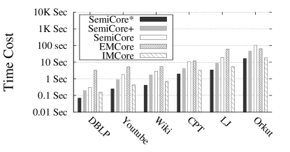
(a) Time Cost (Small Graphs)

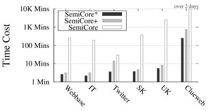
(b) Time Cost (Big Graphs)

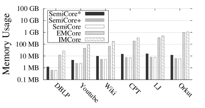
(c) Memory Usage (Small Graphs)

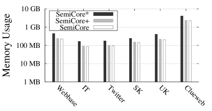
(d) Memory Usage (Big Graphs)

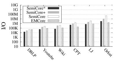
(e) I/Os (Small Graphs)

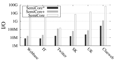
(f) I/Os (Big Graphs)

Figure 9: Core Decomposition on Different Datasets

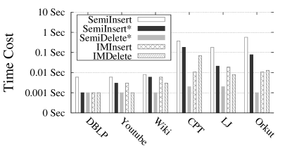
(a) Average Time (Small Graphs)

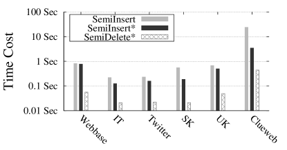
(b) Average Time (Big Graphs)

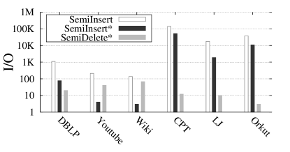
(c) Average I/Os (Small Graphs)

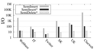
(d) Average I/Os (Big Graphs)

Figure 10: Core Maintenance on Different Datasets

Big Graphs. We report the performance of our algorithms on big graphs in Fig. 9 (b), (d), and (f). The largest dataset $\mathsf{Clueweb}$ contains nearly $1$ billion nodes and $42.6$ billion edges. We can see from Fig. 9 (a) that ${\mathsf{SemiCore}}^{*}$ can process all datasets within $10$ minutes except $\mathsf{Clueweb}$. In Fig. 9, we can see that ${\mathsf{SemiCore}}^{*}$ totally costs less than $4.2$ GB memory to process the largest dataset $\mathsf{Clueweb}$. This result demonstrates that our algorithm can be deploy in any commercial machine to process big graph data. Fig. 9 (f) further reveals the advance of optimization in terms of I/O cost, since ${\mathsf{SemiCore}}^{*}$ spends much less I/Os than ${\mathsf{SemiCore}}$ and ${\mathsf{SemiCore}}^{+}$ in all datasets.

VI-B Core Maintenance

We test the performance of our maintenance algorithms (${\mathsf{SemiInsert}}$, ${\mathsf{SemiInsert}}^{*}$, and ${\mathsf{SemiDelete}}^{*}$). The state-of-the-art streaming in-memory algorithms in [27], denoted by ${\mathsf{IMInsert}}$ and ${\mathsf{IMDelete}}$ are also compared in small graphs. We randomly select $100$ distinct existing edges in the graph for each test. To test the performance of edge deletion, we remove the $100$ edges from the graph one by one and take the average processing time and I/Os. To test the performance of edge insertion, after the $100$ edges are removed, we insert them into the graph one by one and take the average processing time and I/Os. The experimental results are reported in Fig. 10.

From Fig. 10, we can see that ${\mathsf{SemiDelete}}^{*}$ is more efficient than ${\mathsf{SemiInsert}}^{*}$ in both processing time and I/Os for all datasets. This is because ${\mathsf{SemiDelete}}^{*}$ simply follows ${\mathsf{SemiCore}}^{*}$ and does not rely on the calculation of other new graph properties. From Fig. 10 (a), we can find that our core maintenance algorithm ${\mathsf{SemiInsert}}^{*}$ is comparable to the state-of-the-art in-memory algorithm ${\mathsf{IMInsert}}$ for edge insertion. ${\mathsf{SemiDelete}}^{*}$ is even faster than ${\mathsf{IMDelete}}$ for edge deletion. This is due to the simple structures and data access model used in ${\mathsf{SemiDelete}}^{*}$. ${\mathsf{SemiInsert}}^{*}$ outperforms ${\mathsf{SemiInsert}}$ in both processing time and I/Os for all datasets.

(a) Vary $|V|$ ($\mathsf{Twitter}$)

(b) Vary $|V|$ ($\mathsf{UK}$)

(c) Vary $|E|$ ($\mathsf{Twitter}$)

(d) Vary $|E|$ ($\mathsf{UK}$)

Figure 11: Scalability of Core Decomposition

(a) Vary $|V|$ ($\mathsf{Twitter}$)

(b) Vary $|V|$ ($\mathsf{UK}$)

(c) Vary $|E|$ ($\mathsf{Twitter}$)

(d) Vary $|E|$ ($\mathsf{UK}$)

Figure 12: Scalability of Core Maintenance

VI-C Scalability Testing

In this experiment, we test the scalability of our core decomposition and core maintenance algorithms. We choose two big graphs $\mathsf{Twitter}$ and $\mathsf{UK}$ for testing. We vary number of nodes $|V|$ and number of edges $|E|$ of $\mathsf{Twitter}$ and $\mathsf{UK}$ by randomly sampling nodes and edges respectively from 20% to 100%. When sampling nodes, we keep the induced subgraph of the nodes, and when sampling edges, we keep the incident nodes of the edges. Here, we only report the processing time. The memory usage is linear to the number of nodes, and the curves for I/O cost are similar to that of processing time.

Core Decomposition. Fig. 11 (a) and (b) report the processing time of our proposed algorithms for core decomposition when varying $|V|$ in $\mathsf{Twitter}$ and $\mathsf{UK}$ respectively. When $|V|$ increases, the processing time for all algorithms increases. ${\mathsf{SemiCore}}^{*}$ performs best in all cases and is over an order of magnitude faster than ${\mathsf{SemiCore}}$ in both $\mathsf{Twitter}$ and $\mathsf{UK}$. Fig. 11 (a) and (b) show the processing time of our core decomposition algorithms when varying $|E|$ in $\mathsf{Twitter}$ and $\mathsf{UK}$ respectively. When $|E|$ increases, the processing time for all algorithms increases, and ${\mathsf{SemiCore}}^{*}$ performs best among all three algorithms. When $|E|$ increases, the gap between ${\mathsf{SemiCore}}^{*}$ and ${\mathsf{SemiCore}}$ also increases. For example, in $\mathsf{UK}$, when $|E|$ reaches $100\%$, ${\mathsf{SemiCore}}^{*}$ is more than two orders of magnitude faster than ${\mathsf{SemiCore}}$.

Core Maintenance. The scalability testing results for core maintenance are shown in Fig. 12. As shown in Fig. 12 (a) and Fig. 12 (b), when increasing $|V|$ from $20\%$ to $100\%$, the processing time for all algorithms increases. ${\mathsf{SemiDelete}}^{*}$ performs best, and ${\mathsf{SemiInsert}}^{*}$ is faster than ${\mathsf{SemiInsert}}$ for all testing cases. The curves of our core maintenance algorithms when varying $|E|$ are shown in Fig. 12 (c) and Fig. 12 (d) for $\mathsf{Twitter}$ and $\mathsf{UK}$ respectively. ${\mathsf{SemiDelete}}^{*}$ and ${\mathsf{SemiInsert}}^{*}$ are very stable when increasing $|E|$ in both $\mathsf{Twitter}$ and $\mathsf{UK}$, which shows the high scalability of our core maintenance algorithms. ${\mathsf{SemiInsert}}$ performs worst among all three algorithms. When $|E|$ increases, the performance of ${\mathsf{SemiInsert}}$ is unstable because ${\mathsf{SemiInsert}}$ needs to locate a connected component whose size can be very large in some cases.

VII Related Work

Core Decomposition. $k$-core is first introduced in [28]. Batagelj and Zaversnik [9] give an linear in-memory algorithm for core decomposition, which is presented detailed in Section III. This problem is also studied for the weighted graphs [15] and directed graphs [14]. Cheng et al. [11] propose an I/O efficient algorithm for core decomposition. [23] gives a distributed algorithm for core decomposition. Core decomposition in random graphs is studied in [21, 25, 22, 17]. Core decomposition in an uncertain graph is studied in [10]. Locally computing and estimating core numbers are studied in [12] and [24] respectively. [27] and [19] propose in-memory algorithms to maintain the core numbers of nodes in dynamic graphs.

Semi-external Algorithms. Semi-external model, which strictly bounds the memory size, becomes very popular in processing big graphs recently. For example, [32] proposes a semi-external algorithm to find all strong connected components for a massive directed graph. [33] gives semi-external algorithms to compute a DFS tree for a graph in the disk using divide & conquer strategy. [20] studies maximum independent set under the semi-external model.

VIII Conclusions

In this paper, considering that many real-world graphs are big and cannot reside in the main memory of a machine, we study I/O efficient core decomposition on web-scale graphs, which has a large number of applications. The existing solution is not scalable to handle big graphs because it cannot bound the memory size and may load most part of the graph in memory. Therefore, we follow a semi-external model, which can well bound the memory size. We propose an I/O efficient semi-external algorithm for core decomposition, and explore two optimization strategies to further reduce the I/O and CPU cost. We further propose semi-external algorithms and optimization techniques to handle graph updates. We conduct extensive experiments on $12$ real graphs, one of which contains $978.5$ million nodes and $42.6$ billion edges, to demonstrate the efficiency of our proposed algorithm.

References

- [1] A. Aggarwal and S. Vitter, Jeffrey. The input/output complexity of sorting and related problems. Commun. ACM, 31(9), 1988.
- [2] M. Altaf-Ul-Amine, K. Nishikata, T. Korna, T. Miyasato, Y. Shinbo, M. Arifuzzaman, C. Wada, M. Maeda, T. Oshima, H. Mori, and S. Kanaya. Prediction of protein functions based on k-cores of protein-protein interaction networks and amino acid sequences. Genome Informatics, 14, 2003.
- [3] J. I. Alvarez-Hamelin, L. Dall’Asta, A. Barrat, and A. Vespignani. k-core decomposition: a tool for the visualization of large scale networks. CoRR, abs/cs/0504107, 2005.
- [4] J. I. Alvarez-Hamelin, L. Dall’Asta, A. Barrat, and A. Vespignani. Large scale networks fingerprinting and visualization using the k-core decomposition. In Proc. of NIPS’05, 2005.
- [5] J. I. Alvarez-Hamelin, L. Dall’Asta, A. Barrat, and A. Vespignani. How the k-core decomposition helps in understanding the internet topology. In ISMA Workshop on the Internet Topology, volume 1, 2006.
- [6] R. Andersen and K. Chellapilla. Finding dense subgraphs with size bounds. In Algorithms and Models for the Web-Graph. 2009.
- [7] G. Bader and C. Hogue. An automated method for finding molecular complexes in large protein interaction networks. BMC Bioinformatics, 4(1), 2003.
- [8] B. Balasundaram, S. Butenko, and I. V. Hicks. Clique relaxations in social network analysis: The maximum k-plex problem. Operations Research, 59(1), 2011.
- [9] V. Batagelj and M. Zaversnik. An o(m) algorithm for cores decomposition of networks. CoRR, cs.DS/0310049, 2003.
- [10] F. Bonchi, F. Gullo, A. Kaltenbrunner, and Y. Volkovich. Core decomposition of uncertain graphs. In Proc. of KDD’14, 2014.
- [11] J. Cheng, Y. Ke, S. Chu, and M. T. Özsu. Efficient core decomposition in massive networks. In Proc. of ICDE’11, 2011.
- [12] W. Cui, Y. Xiao, H. Wang, and W. Wang. Local search of communities in large graphs. In Proc. of SIGMOD’14, 2014.
- [13] S. N. Dorogovtsev, A. V. Goltsev, and J. F. F. Mendes. K-core organization of complex networks. Physical review letters, 96(4), 2006.
- [14] C. Giatsidis, D. M. Thilikos, and M. Vazirgiannis. D-cores: Measuring collaboration of directed graphs based on degeneracy. In Proc. of ICDM’11, 2011.
- [15] C. Giatsidis, D. M. Thilikos, and M. Vazirgiannis. Evaluating cooperation in communities with the k-core structure. In Proc. of ASONAM’11, 2011.
- [16] J. Healy, J. Janssen, E. Milios, and W. Aiello. Characterization of graphs using degree cores. In Algorithms and Models for the Web-Graph. 2008.
- [17] S. Janson and M. J. Luczak. A simple solution to the k-core problem. Random Struct. Algorithms, 30(1-2), 2007.
- [18] R. Li, L. Qin, J. X. Yu, and R. Mao. Influential community search in large networks. PVLDB, 8(5), 2015.
- [19] R. Li, J. X. Yu, and R. Mao. Efficient core maintenance in large dynamic graphs. IEEE Trans. Knowl. Data Eng., 26(10), 2014.
- [20] Y. Liu, J. Lu, H. Yang, X. Xiao, and Z. Wei. Towards maximum independent sets on massive graphs. PVLDB, 8(13), 2015.
- [21] T. Luczak. Size and connectivity of the k-core of a random graph. Discrete Math., 91(1), 1991.
- [22] M. Molloy. Cores in random hypergraphs and boolean formulas. Random Struct. Algorithms, 27(1), 2005.
- [23] A. Montresor, F. De Pellegrini, and D. Miorandi. Distributed k-core decomposition. TPDS, 24(2), 2013.
- [24] M. P. O’Brien and B. D. Sullivan. Locally estimating core numbers. In Proc. of ICDM’14, 2014.
- [25] B. Pittel, J. Spencer, and N. Wormald. Sudden emergence of a giant k-core in a random graph. J. Comb. Theory Ser. B, 67(1), 1996.
- [26] L. Qin, R. Li, L. Chang, and C. Zhang. Locally densest subgraph discovery. In Proc. of KDD’15, 2015.
- [27] A. E. Saríyüce, B. Gedik, G. Jacques-Silva, K.-L. Wu, and U. V. Çatalyürek. Streaming algorithms for k-core decomposition. PVLDB, 6(6), 2013.
- [28] S. B. Seidman. Network structure and minimum degree. Social networks, 5(3), 1983.
- [29] M. Sozio and A. Gionis. The community-search problem and how to plan a successful cocktail party. In Proc. of KDD’10, 2010.
- [30] A. Verma and S. Butenko. Network clustering via clique relaxations: A community based approach. Graph Partitioning and Graph Clustering, 588, 2012.
- [31] H. Zhang, H. Zhao, W. Cai, J. Liu, and W. Zhou. Using the k-core decomposition to analyze the static structure of large-scale software systems. The Journal of Supercomputing, 53(2), 2010.
- [32] Z. Zhang, J. X. Yu, L. Qin, L. Chang, and X. Lin. I/O efficient: computing sccs in massive graphs. In Proc. of SIGMOD’13, 2013.
- [33] Z. Zhang, J. X. Yu, L. Qin, and Z. Shang. Divide & conquer: I/O efficient depth-first search. In Proc. of SIGMOD’15, 2015.