Ground-state phase diagram of the quantum Rabi model

Abstract

The Rabi model plays a fundamental role in understanding light-matter interaction. It reduces to the Jaynes-Cummings model via the rotating-wave approximation, which is applicable only to the cases of near resonance and weak coupling. However, recent experimental breakthroughs in upgrading light-matter coupling order require understanding the physics of the full quantum Rabi model (QRM). Despite the fact that its integrability and energy spectra have been exactly obtained, the challenge to formulate an exact wavefunction in a general case still hinders physical exploration of the QRM. Here we unveil a ground-state phase diagram of the QRM, consisting of a quadpolaron and a bipolaron as well as their changeover in the weak-, strong- and intermediate-coupling regimes, respectively. An unexpected overweighted antipolaron is revealed in the quadpolaron state, and a hidden scaling behavior relevant to symmetry breaking is found in the bipolaron state. An experimentally accessible parameter is proposed to test these states, which might provide novel insights into the nature of the light-matter interaction for all regimes of the coupling strengths.

Introduction.– In the past decade, it has been witnessed that the exploration of fundamental quantum physics in light-matter coupling systems has significantly evolved toward the (ultra-)strong coupling regime Wallraff2004 ; Gunter2009 ; Niemczyk2010 ; Peropadre2010 ; Forn-Diaz2010 ; Cristofolini2012 ; Scalari2012 ; Xiang2013 . For example, in 2004, the strong coupling of a single microwave photon to a superconducting qubit was realized experimentally by using circuit quantum electrodynamics Wallraff2004 . In 2010, this coupling rate was enhanced to reach a considerable fraction up to 12% of the cavity transition frequencyNiemczyk2010 . Even with such small fractions the system has already entered into so-called ultrastrong-coupling limitCiuti2006 ; Devoret2007 . In this situation, the well-known Jaynes-Cummings (JC) modelJC1963 is no longer applicable because the JC model is valid only in the cases of near resonance and weak coupling Allen1987 . Indeed, the experimentally observed anticrossing in the cavity transmission spectra Niemczyk2010 was due to counter-rotating terms, which are dropped in the JC model as a rotating-wave approximation. In addition, experimental observation of the Bloch-Siegert shift Forn-Diaz2010 also requires taking into account the counter-rotating terms in the description of the JC model. Thus the importance of the counter-rotating terms raises requests to comprehend the behavior of a full quantum Rabi model rabi1936 ; rabi1937 ; Cohen1992 (QRM) for all regimes of the coupling strengths Ciuti2005 ; Bourassa2009 ; Casanova2010 ; Irish2014 .

Remarkably, an important progress in the study of the QRM in the past years is the proof of its integrability Braak2011 ; Solano2011 . As a result, its energy spectra have been exactly obtained Braak2011 ; Chen2012 . However, to calculate the dynamics of the system, correlation functions, and even other simpler physical observables, it is not enough to know only the exact eigenvalues, but the wavefunctions (e.g., the exact eigenstates) are desirable. Based on series expansions of the eigenstates in terms of known basis sets, it was realized that a standard calculation with double precision, sufficient to compute the spectrum, fails for the eigenstatesWolf2012 . Therefore, the challenge to formulate an exact wave function in a general case still hampers access to a full understanding of the QRM.

In this work, by deforming the polaron and antipolaron Bera2014a ; Bera2014b we propose a novel variational wavefunction ansatz to extract the ground state physics of the QRM. It is found that this ansatz is valid with high accuracy in all regimes of the coupling strengths. Thus a ground state phase diagram of the QRM is constructed. The nature of the system variation, by increasing the coupling strength from weak to strong, becomes transparent in the ground-state phase diagram with a quantum state changeover from quadpolaron to bipolaron, around a novel critical-like coupling scale analytically extracted. In particular, an unexpected overweighted antipolaron is revealed in the quadpolaron state and a hidden scaling behavior is found in the bipolaron state. Moreover, we propose an experimentally accessible parameter to test these states. For perspective, we also extend this ansatz to the multiple-mode case, which is expected to be useful to understand the physics of the spin-boson model Spin-Boson .

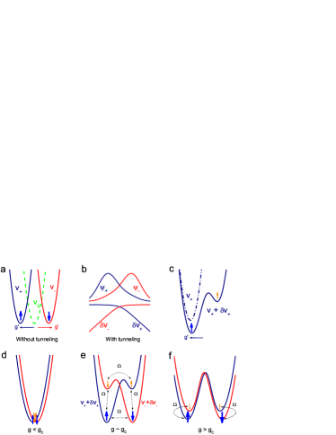
Figure 1: (Color) Schematic diagram for effective potentials induced by the tunneling between two levels. a, In the absence of tunneling, i.e., $\Omega=0$, the original harmonic oscillator ($v_{0}$) is coupled with two levels denoted by $\uparrow$ and $\downarrow$ to form two polarons (associated with $v_{\pm}$) with the left($+,\uparrow$) and right($-,\downarrow$) displacement $g^{\prime}=\sqrt{2}g/\omega$. b, When the tunneling $\Omega$ is switched on, the left- and right-polarons provide an effective potential for each other $\delta v_{\pm}=\eta{\frac{\Omega}{\omega}}\frac{\psi_{\mp}}{\psi_{\pm}}$ ($\eta=\pm$ represents the parity, here we focus on the ground state with “$-$” parity), which induces an antipolaron, as shown in c. c, The potential of the left-polaron deforms from $v_{+}$ to $v_{+}+\delta v_{+}$. The size of $\uparrow$ indicates the weight of the polaron (blue) and antipolaron (orange), respectively, in the same and opposite directions of the potential displacement. The situation is symmetric for the right-polaron. d-f, Typical deformed potentials in the weak ($g<g_{c}$), intermediate ($g\sim g_{c}$), and strong coupling ($g>g_{c}$) cases. There exist four tunneling channels between $\uparrow$ and $\downarrow$ states, as shown in e, forming a quadpolaron state. In the strong coupling case, the tunneling between left and right states decays until it is vanishingly small due to the large potential barriers between them, yielding a bipolaron state in f.

The model and effective potential.– The QRM rabi1936 ; rabi1937 describes a quantum two-level system coupled to a single bosonic mode or quantized harmonic oscillator, which is a paradigm for interacting quantum systems ranging from quantum optics cavityQED to quantum information raimond to condensed matter holstein . The model Hamiltonian reads

$$H=\omega a^{\dagger}a+\frac{\Omega}{2}\sigma_{x}+g\sigma_{z}(a^{\dagger}+a),$$ (1)

where $a^{\dagger}(a)$ is the bosonic creation (annihilation) operator with frequency $\omega$ and $\sigma_{x,z}$ is the Pauli matrix with level splitting $\Omega$. The last term describes the interaction with coupling strength $g$.

In terms of the quantum harmonic oscillator with dimensionless formalismMahan2000 $a^{\dagger}=\left(\hat{x}-i\hat{p}\right)/\sqrt{2}$, $a=\left(\hat{x}+i\hat{p}\right)/\sqrt{2}$, where $\hat{x}=x$ and $\hat{p}=-i\frac{\partial}{\partial x}$ are the position and momentum operators, respectively, the model can be rewritten as

$$H=\sum_{\sigma_{z}=\pm}\left(h^{\sigma_{z}}|\sigma_{z}\rangle\langle\sigma_{z}|+{\frac{\Omega}{2}}|\sigma_{z}\rangle\langle\overline{\sigma}_{z}|\right)+{\cal E}_{0},$$ (2)

where $\overline{\sigma}_{z}=-\sigma_{z}$ and $+$($-$) labels the up $\uparrow$ (down $\downarrow$) spin in the $z$ direction, respectively. $h^{\pm}=\frac{1}{2}\omega(\hat{p}^{2}+v_{\pm})$, with $v_{\pm}=\left(\hat{x}\pm g^{\prime}\right)^{2}$ and $g^{\prime}=\sqrt{2}g/\omega$, while ${\cal E}_{0}=-\frac{1}{2}\omega(g^{\prime 2}+1)$ is a constant energy. Apparently, $h^{\pm}$ define two bare polarons Bera2014a ; Bera2014b in the sense that the harmonic oscillator is bound by $\sigma_{z}$ due to the coupling $g^{\prime}$, as shown in Fig. 1a. These two polarons form two bare potential wells but the existence of the level splitting $\Omega$ (resulting in the tunneling between these two wellsIrish2014 ) makes the model difficult to solve analytically.

Let us begin with the wave-function $\Psi$ satisfying the Schrödinger equation $H\Psi=E\Psi$ with the eigenenergy $E$. Due to the fact that the model possesses the parity symmetry, namely, $[{\cal P},H]=0$ with ${\cal P}=\sigma_{x}(-1)^{a^{\dagger}a}$, $\Psi$ should take the form of $\Psi=\frac{1}{\sqrt{2}}\left(\psi_{+}|\uparrow\rangle+\eta\psi_{-}|\downarrow\rangle\right)$, where $\psi_{\pm}=\psi(\pm x)$ will be given below and $\eta=1$ $(-1)$ for positive (negative) parity. Without loss of generality, here we consider the ground state, with negative parity. The Schrödinger equation becomes

$$\frac{1}{2}\omega(\hat{p}^{2}+v_{\pm}+\delta v_{\pm})\psi_{\pm}=E\psi_{\pm},$$ (3)

where $\delta v_{\pm}=-\frac{\Omega}{\omega}\frac{\psi_{\mp}}{\psi_{\pm}}$ is an additional effective potential originating from the tunneling, as shown in the lower panel of Fig. 1b. The additional potential will deform the bare potential and as a result creates a subwell in the opposite direction of the bare potential $v_{\pm}$, as illustrated in Fig. 1c. The subwell induces an antipolaron as a quantum effect. The above analysis from potential subwell verifies the existence of antipolaron from wavefunction expansionBera2014a ; Bera2014b . Thus, the polaron and antipolaron constitute the basic ingredients of the ground-state wavefunction.

Deformed polaron and antipolaron.– With the concept of polaron and antipolaron in hand, the competition between different energy scales $\omega,\Omega$ and $g^{\prime}$ involved in the QRM will inevitably lead to deformations of the polaron and antipolaron. Physically, they can deform predominantly in two possible ways: the position is shifted and the frequency is renormalized, which will introduce four independent variational parameters given below. Explicit deformation depends on the coupling strength once the tunneling is fixed, as shown in Fig. 1 d-f from weak to strong couplings according to a critical-like coupling strength $g_{c}$. Thus a trial variational wave-function for $\psi(x)$ takes the superposition of the deformed polaron ($\varphi_{\alpha}$) and antipolaron ($\varphi_{\beta}$),

$$\psi(x)=\alpha\varphi_{\alpha}(x)+\beta\varphi_{\beta}(x),$$ (4)

where $\varphi_{\alpha}(x)=\phi_{0}\left(\xi_{\alpha}\omega,x+\zeta_{\alpha}g^{\prime}\right)$ and $\varphi_{\beta}(x)=\phi_{0}\left(\xi_{\beta}\omega,x-\zeta_{\beta}g^{\prime}\right)$, with $\phi_{0}(\omega,x)$ being the ground-state of standard harmonic oscillator with frequency $\omega$. Here $\xi_{i}$ ($\zeta_{i}$), with $i=\alpha$ and $\beta$, describes the renormalization for frequency (displacement) independently for the polaron and the antipoalron, while the coefficients of $\alpha$ and $\beta$ denote their weights, subject to the normalization condition $\langle\psi|\psi\rangle=1$. We stress that in contrast to the direct expansion on basis series without frequency renormalization Bera2014a ; Bera2014b , we design our trial wavefunction based on the dominant physics of deformation.

It turns out that our variational wavefunction is capable of providing a reliable analysis on the QRM in the whole parameter regime, ranging from weak to strong couplings, as shown for several physical quantities for the ground-state including the energy, the mean photon number, the coupling correlation and the tunneling strength in Appendix A. Obviously the remarkable agreement between our results and the exact ones roots in the fact that our trial wavefunction correctly captures the basic physics, as illustrated by the accurate wavefunction profiles compared to the exact numerical ones for various couplings in Fig.2a. The variational wavefunction, with its concise physical ingredients and its accuracy, in turn facilitates unveiling more underlying physics.

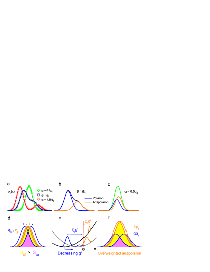
Figure 2: (Color) Mechanism for overweighted antipolaron in quadpolaron state. a, The calculated (solid lines) spin-up groundstate wavefunctions, $\psi_{+}(x)=\alpha\varphi_{\alpha}(x)+\beta\varphi_{\beta}(x)$, at $g/g_{c}=0.5,1.,1.25$ respectively, for weak (green), intermediate(navy), and strong(red) couplings, with $\omega/\Omega=0.1$. The symbols denote the numerical exact results. The spin-down wavefunction is given by $-\psi_{+}(-x)$(not shown). b and c, $\alpha$- and $\beta$-components of $\psi_{+}(x)$, which correspond to the polaron(blue) and antipolaron(orange), respectively, for the intermediate $g\sim g_{c}$ and weak $g=0.5g_{c}$ coupling cases. d, The overlaps between different polarons and/or antipolarons without the weights, $S_{i\bar{j}}=\langle\varphi_{i}(x)|\varphi_{j}(-x)\rangle$ with $i,j=\alpha,\beta$. It is clear that $S_{\beta\bar{\beta}}(\text{yellow})>S_{\alpha\bar{\alpha}}(\text{light magenta})$. e, Schematic illustration of the physics for the overweighted antipolaron. When decreasing the coupling strength $g^{\prime}$, the potential provided by the left-displaced oscillator for the antipolaron gets lower, so the tunneling energy gain from large $S_{\beta\bar{\beta}}$ in d overwhelms the potential cost, which favors a larger weight of antipolaron. f, The overweighted antipolaron with a larger weight than the polaron.

Quadpolaron/bipolaron quantum state changeover.– From Fig.2a-c one sees that when increasing the coupling, the wavepacket splits into visible polaron and antipolaron (see animated plots in Supplementary Material for more vivid evolutions of potentials and wavepackets). Before the full splitting, there are significant tunnelings in all the four channels between the polarons and antipolarons, as schematically shown in Fig. 1e. Thus, in this sense we call this state a quadpolaron. After the splitting, only two same-side channels of tunneling survives while the left-right channels are blocked gradually by the increasing barrier, as sketched in Fig. 1f. This state is termed here as a bipolaron. Despite the evolution from a transition-like feature in the low frequency limit to a crossover behavior in finite frequencies for the changover between quadpolaron and bipolaron states, the nature of the afore-mentioned splitting is essentially the same. This enables us to obtain an analytic coupling scale (see Appendix B), $g_{c}=\sqrt{\omega^{2}+\sqrt{\omega^{4}+g^{4}_{c0}}}$, which generalizes the low frequency-limit resultAshhab2010 $g_{c0}=\sqrt{\omega\Omega}/2$ and correctly captures the quantum state changeover between quadpolaron and bipolaron for the whole range of frequencies.

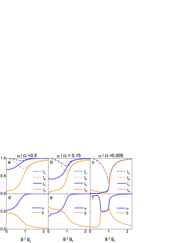
Figure 3: (Color) Renormalization factor and weight as a function of the coupling strength $g$. $\zeta_{i}$ ($i=\alpha,\beta$) is the displacement renormalization and $\xi_{i}$ is the frequency renormalization. $\alpha$ and $\beta$ denote the weights of the polaron and the antipolaron, respectively, in the variational groundstate wavefunction. a and d, $\omega/\Omega=0.5$. b and e, $\omega/\Omega=0.15$. c and f, $\omega/\Omega=0.005$.

Quadpolaron asymmetry and overweighted antipolaron in the regime of $g\lesssim g_{c}$.– We find that the polaron and antipolaron in the quadpolaron state have asymmetric displacements, which leads to a subtle competition depending on the frequency $\omega/\Omega$. Figure 3 shows three types of distinct behaviors of the variational parameters in three different frequency regimes: high frequency ($\omega/\Omega\gtrsim 0.47$), intermediate frequency($\omega/\Omega\in[0.07,0.47]$), and low frequency ($\omega/\Omega\lesssim 0.07$). The result is understandable due to the fact that the antipolaron always has a higher potential energy owing to its opposite direction to the displacement of $v_{\pm}$. Roughly speaking, at a high frequency, the antipolaron should have a lower weight than the polaron ($\beta<\alpha$) since the antipolaron is suppressed by the high potential. At a low frequency, the polaron benefits from both potential and tunneling energies. However, competition becomes subtle at an intermediate frequency as each of these different energy scales may only favor either the polaron or the antipolaron respectively, which may lead to overweighted antipolaron, as shown in Fig.3e.

Below we give a more explicit analysis. Actually, the four channel tunneling energies in the quadpolaron are proportional to the overlaps of the polarons and antipolarons, $S_{\alpha\bar{\alpha}}$, $S_{\beta\bar{\beta}}$, $S_{\alpha\bar{\beta}}$ and $S_{\beta\bar{\alpha}}$, respectively, as shown in Fig.2d. The mixture terms $S_{\alpha\bar{\beta}}$ and $S_{\beta\bar{\alpha}}$ do not affect the weight competition between the polaron and antipolaron, while $S_{\alpha\bar{\alpha}}$ and $S_{\beta\bar{\beta}}$ yield imbalances. Indeed, the antipolarons have larger overlap than the polarons, i.e. $S_{\beta\bar{\beta}}>S_{\alpha\bar{\alpha}}$ (see Fig. 2d). This is because the antipolarons in up and down spins are closer to each other than the polarons in order to reduce their higher potential energy, as indicated in Fig. 2e and quantitatively shown by $\zeta_{\beta}<\zeta_{\alpha}$ in Fig. 3a and 3b. Therefore, as far as the tunneling is concerned, it would tend to have more weight of antipolarons to gain a maximum tunneling. When the intermediate frequency reduces the cost of potential energy for such tendency, a larger antipolaron weight might finally occur, as in Fig. 2f, leading to an unexpected overweighted antipolaron. We find that this really occurs as demonstrated in Fig. 3e where a weight reversion appears at the crossing of $\alpha$ and $\beta$ for a weaker coupling.

At the low frequency, the harmonic potential becomes very flat, the polarons may get closer than antipolarons, as indicated by $\zeta_{\alpha}<\zeta_{\beta}$ in Fig.3c in the weak coupling regime. In this case, $S_{\alpha\bar{\alpha}}$ is greater than $S_{\beta\bar{\beta}}$ so that polarons have favorable energies in both potential and tunneling. Thus the polaron regains its priority in weight.

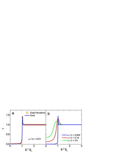
Figure 4: (Color) Scaling quantity $\gamma$ as a function of the coupling strength $g$. a, Our results compared with exact numerics at $\omega/\Omega=0.01$ as an example. b, $\gamma$ for different values of the ratios $\omega/\Omega$. The scaling relation $\zeta_{i}\doteq\xi_{i}$ is tested by $\gamma=1$ beyond $g_{c}$.

Bipolaron and hidden scaling behavior in the regime of $g\gtrsim g_{c}$.– In the bipolaron regime, the remaining tunneling in channels $S_{\alpha\bar{\beta}}$ and $S_{\beta\bar{\alpha}}$ leads to intriguing physics, showing a deeper nature of the interaction in the symmetry breaking aspect. Indeed, Fig.3a-c show that in this regime the frequency factor $\xi_{i}$ and the displacement factor $\zeta_{i}$ collapse into the same value, i.e $\zeta_{i}\doteq\xi_{i}$. In fact, due to vanishing photon number below $g_{c}$ at low frequency limit, the parity ${\cal P}$ can be decomposed into separate spin and spatial reversal sub-symmetries which are broken beyond $g_{c}$. However, further seeking the symmetry breaking character from these sub-symmetries would fail at finite frequencies due to emergence of a finite number of photons below $g_{c}$. Nevertheless, the $\zeta_{i}$-$\xi_{i}$ symmetric aspect revealed here provides a compensation, from the beyond-$g_{c}$ side instead but valid also for finite frequencies. To test this scaling behavior, we propose an experimentally accessible quantity, $\gamma\equiv\frac{\omega}{gt}\sqrt{\langle a^{+}a\rangle-\frac{1}{4}(t+t^{-1})+\frac{1}{2}}$, where $t=-\langle\left(a^{+}-a\right)^{2}\rangle$, which becomes the scaling ratio $\gamma\rightarrow\zeta/\xi$ (see Appendix C) for their average $\xi=\left(\xi_{\alpha}+\xi_{\beta}\right)/2$ and $\zeta=\left(\zeta_{\alpha}+\zeta_{\beta}\right)/2$ and thus equals to one above $g_{c}$, as shown in Fig. 4 for various frequencies. The experimental measurement of $\gamma$ thus provides a possible way to distinguish the states of bipolaron and quadpolaron as well as their changeover.

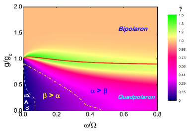
Figure 5: (Color) An overview of ground-state phase diagram for the QRM. Quadpolaron ($g\lesssim g_{c}$) and bipolaron ($g\gtrsim g_{c}$) as well as their crossover near the minimum of $\xi_{i}$ (red solid line) or the maximum of $\gamma$ around analytic $g_{c}$. The quadpolaron regime is further divided into the normal ($\alpha>\beta$) and overweighted antipolaron ($\alpha<\beta$) regimes. The dashed and dot-dashed lines have been obtained numerically from the cross points as shown in Fig. 3 (e) and (f). The color density for $\gamma$ further distinguishes the characters of the different regimes and their changeovers.

Ground-state phase diagram.– The above discussions on polaron-antipolaron competition can be summarized into a ground-state phase diagram unveiled, as shown in Fig. 5. The ground-state with different channels of tunneling is identified as a quadpolaron when $g\lesssim g_{c}$ and as a bipolaron when $g\gtrsim g_{c}$. An overweighted antipolaron is hidden in the quadpolaron regime, while a scaling relation between the displacement and frequency renormalizations is revealed in the bipolaron regime. Note that the polaron and antipolaron structures might be detected by optomechanicsRestrepo2014 ; Meystre2013 and $\gamma$ is experimentally measurable. The diagram may provide a renewed panorama for deeper theoretical investigations and may raise more challenges for experiments.

Perspective in multiple modes.– The basic physics in the QRM has a profound implication for the spin-boson modelSpin-Boson , which is a multiple-mode version of the QRM. The essential variational ingredients remain similar. The trial wavefunction can be written as $\psi[\{x_{k}\}]=\alpha\prod_{k=1}^{M}\varphi_{\alpha}^{k}+\beta\prod_{k=1}^{M}\varphi_{\beta}^{k}$ with the extension $\{\omega,g,x,\xi_{i},\zeta_{i}\}\rightarrow\{\omega_{k},g_{k},x_{k},\xi^{k}_{i},\zeta^{k}_{i}\}$ for the $k$’th mode. We illustrate the same accuracy by a two-mode case in Appendix D.

Acknowledgements.– We thank Jun-Hong An for helpful discussions. Work at CSRC and Lanzhou University was supported by National Natural Science Foundation of China, PCSIRT (Grant No. IRT1251), National “973” projects of China. Z.-J.Y. also acknowledges partial financial support from the Future and Emerging Technologies (FET) programme within the Seventh Framework Programme for Research of the European Commission, under FET-Open grant number: 618083 (CNTQC).

Appendix A Variational method and physical properties

Here we calculate the ground-state physical properties from the variational method, including the energy $E$, the mean photon number $\langle a^{\dagger}a\rangle$, the coupling correlation $\langle\sigma_{z}(a^{\dagger}+a)\rangle$ and the spin flipping (tunneling) strength $\langle\sigma_{x}\rangle$.

A.1 The energy

As introduced in the main part of the paper, the wavefunction for the reformulated Hamiltonian (2) has the following form

$$\Psi=\frac{1}{\sqrt{2}}\left(\psi_{+}(x)\mid\uparrow\rangle+\eta\psi_{-}(x)\mid\downarrow\rangle\right),$$ (5)

where $\eta=\pm$ is the parity. We adopt the variational trial wavefunction as a superposition of the polaron and the antipolaron

$$\psi_{+}(x)=\psi_{-}(-x)=\alpha\varphi_{\alpha}\left(x\right)+\beta\varphi_{\beta}\left(x\right),$$ (6)

where

$$\varphi_{\alpha}\left(x\right)=\phi_{n}(\xi_{\alpha}\omega,x+\zeta_{\alpha}g^{\prime}),$$ (7)

$$\varphi_{\beta}\left(x\right)=\phi_{n}(\xi_{\beta}\omega,x-\zeta_{\beta}g^{\prime}),$$ (8)

with $\phi_{n}(\omega,x)$ being the $n$’th eigenstate of the standard quantum harmonic oscillator with frequency $\omega$. In this work we focus on the ground state so that $n=0$ and $\eta=-$. The displacement of the bare potential $v_{\pm}=\left(\hat{x}\pm g^{\prime}\right)^{2}$ in the single-well energy $h^{\pm},$

$$g^{\prime}=\sqrt{2}g/\omega,$$ (9)

is driven by the interaction $g$ and for simplicity we have assumed the unit $\hbar=m=1$. Note that the polaron (antipolaron) has a displacement in the same (opposite) direction as (to) that of the bare potential $v^{\pm}$. The interplay of the interaction and the tunneling leads to the deformation of the wavepacket: the frequency of the polaron (antipolaron) is renormalized by $\xi_{\alpha}$ ($\xi_{\beta}$) and the displacement by $\zeta_{\alpha}$ ($\zeta_{\beta}$), respectively. The weights of the polaron and the antipolaron are subject to the normalization condition $\langle\Psi\left|\Psi\right\rangle=\langle\psi_{+}|\psi_{+}\rangle=1$. These deformation parameters, independently $\{\xi_{\alpha},\xi_{\beta},\zeta_{\alpha},\zeta_{\beta},\alpha\}$, are optimized by minimization of the total energy formulated in the following.

The energy can be directly obtained as

$$E\equiv\left\langle\Psi\right|H\left|\Psi\right\rangle=h_{++}^{+}+\eta\frac{\hbar\Omega}{2}n_{+-}+{\cal E}_{0},$$ (10)

where

$$h_{++}^{+} = \left\langle\psi_{+}\right|h^{+}\left|\psi_{+}\right\rangle$$ (11)

$$= \alpha^{2}h_{\alpha\alpha}^{+}+\beta^{2}h_{\beta\beta}^{+}+2\alpha\beta h_{\alpha\beta}^{+},$$

$$n_{+-} = \langle\psi_{+}|\psi_{-}\rangle$$ (12)

$$= \alpha^{2}S_{\alpha\bar{\alpha}}+\beta^{2}S_{\beta\bar{\beta}}+2\alpha\beta S_{\alpha\bar{\beta}},$$

contribute to the single-well energy and the tunneling energy, respectively. Here, we have defined

$$h_{ij}^{+} = \langle\varphi_{i}\left(x\right)|h^{+}|\varphi_{j}\left(x\right)\rangle,$$

$$S_{ij} = \langle\varphi_{i}\left(x\right)\mid\varphi_{j}\left(x\right)\rangle,$$ (13)

$$S_{i\,\bar{j}} = \langle\varphi_{i}\left(x\right)\mid\varphi_{j}\left(-x\right)\rangle,$$

for $i=\alpha,\beta$, while ${\cal E}_{0}=-\frac{1}{2}\omega(1+g^{\prime 2})$ is a constant energy. Explicit formulas for these quantities are readily available. In this Section we give the result for the ground state

$$h_{\alpha\alpha}^{+} = \frac{1}{2}\omega\left[\frac{1}{2}(\xi_{\alpha}+\xi_{\alpha}^{-1})+\left(1-\zeta_{\alpha}\right)^{2}g^{\prime 2}\right],$$ (14)

$$h_{\beta\beta}^{+} = \frac{1}{2}\omega\left[\frac{1}{2}(\xi_{\beta}+\xi_{\beta}^{-1})+\left(1-\zeta_{\beta}\right)^{2}g^{\prime 2}\right],$$ (15)

$$h_{\alpha\beta}^{+} = \frac{1}{2}\omega\left[\left(1-\xi_{\alpha}^{2}\right)\left\langle\hat{x}_{\alpha}^{2}\right\rangle_{\alpha\beta}+\left(1-\zeta_{\alpha}\right)\left\langle\hat{x}_{\alpha}\right\rangle_{\alpha\beta}2g^{\prime}\right.$$ (16)

$$\left.+\xi_{\alpha}S_{\alpha\beta}+\left(1-\zeta_{\alpha}\right)^{2}g^{\prime 2}S_{\alpha\beta}\right],$$

where

$$\left\langle\hat{x}_{\alpha}\right\rangle_{\alpha\beta} = S_{\alpha\beta}\frac{\left(\zeta_{\alpha}+\zeta_{\beta}\right)\xi_{\beta}}{\left(\xi_{\alpha}+\xi_{\beta}\right)}g^{\prime},$$ (17)

$$\left\langle\hat{x}_{\alpha}^{2}\right\rangle_{\alpha\beta} = \frac{S_{\alpha\beta}}{(\xi_{\alpha}+\xi_{\beta})}\left[1+\frac{\left(\zeta_{\alpha}+\zeta_{\beta}\right)^{2}\xi_{\beta}^{2}}{(\xi_{\alpha}+\xi_{\beta})}g^{\prime 2}\right]$$ (18)

and

$$S_{\alpha\beta} = S(\zeta_{\alpha},\zeta_{\beta},\xi_{\alpha},\xi_{\beta}),$$

$$S_{\alpha\bar{\beta}} = S(\zeta_{\alpha},-\zeta_{\beta},\xi_{\alpha},\xi_{\beta}),$$

$$S_{\alpha\bar{\alpha}} = S(\zeta_{\alpha},\zeta_{\alpha},\xi_{\alpha},\xi_{\alpha}),$$

$$S_{\beta\bar{\beta}} = S(\zeta_{\beta},\zeta_{\beta},\xi_{\beta},\xi_{\beta}),$$ (19)

are given by the function

$$S(\zeta_{1},\zeta_{2},\xi_{1},\xi_{2}) = \exp\left(-\frac{\left(\zeta_{1}+\zeta_{2}\right)^{2}g^{\prime 2}\xi_{1}\xi_{2}}{2(\xi_{1}+\xi_{2})}\right)$$ (20)

$$\times\sqrt{2}\left[\frac{\xi_{1}\xi_{2}}{(\xi_{1}+\xi_{2})^{2}}\right]^{1/4}.$$

A.2 The mean photon number

From the relation

$$a^{\dagger}a=\frac{h^{0}}{\omega}-\frac{1}{2},\quad h^{0}\equiv\frac{1}{2}\omega\left(\hat{p}^{2}+\hat{x}^{2}\right),$$ (21)

and the symmetric relation $\psi_{-}\left(x\right)=\psi_{+}\left(-x\right)$, the mean photon number simply reads as

$$\langle a^{\dagger}a\rangle\equiv\left\langle\Psi\right|a^{\dagger}a\left|\Psi\right\rangle=\frac{h_{++}^{0}}{\omega}-\frac{1}{2}$$ (22)

where

$$h_{++}^{0}=\left\langle\psi_{+}\right|h^{0}\left|\psi_{+}\right\rangle=\alpha^{2}h_{\alpha\alpha}^{0}+\beta^{2}h_{\beta\beta}^{0}+2\alpha\beta h_{\alpha\beta}^{0}.$$ (23)

For the ground state

$$h_{\alpha\alpha}^{0} = \frac{1}{2}\omega\left[\frac{1}{2}(\xi_{\alpha}^{-1}+\xi_{\alpha})+2\zeta_{\alpha}^{2}g^{\prime 2}\right],$$ (24)

$$h_{\beta\beta}^{0} = \frac{1}{2}\omega\left[\frac{1}{2}(\xi_{\beta}^{-1}+\xi_{\beta})+2\zeta_{\beta}^{2}g^{\prime 2}\right],$$ (25)

$$h_{\alpha\beta}^{0} = \frac{1}{2}\omega\left[\left(1-\xi_{\alpha}^{2}\right)\left\langle\hat{x}_{\alpha}^{2}\right\rangle_{\alpha\beta}-\zeta_{\alpha}\left\langle\hat{x}_{\alpha}\right\rangle_{\alpha\beta}2g^{\prime}\right.$$ (26)

$$\left.+\xi_{\alpha}S_{\alpha\beta}+\zeta_{\alpha}^{2}g^{\prime 2}S_{\alpha\beta}\right],$$

and $\left\langle\hat{x}_{\alpha}^{2}\right\rangle_{\alpha\beta}$, $\left\langle\hat{x}_{\alpha}\right\rangle_{\alpha\beta}$ are given by (17) and (18).

A.3 The coupling correlation $\langle\sigma_{z}(a^{\dagger}+a)\rangle$ and the spin flipping (tunneling) strength $\langle\sigma_{x}\rangle$

Now we calculate the coupling correlation $\langle\sigma_{z}(a^{\dagger}+a)\rangle$. Since $(a^{\dagger}+a)=\sqrt{2}\hat{x}$, we have

$$\langle\sigma_{z}(a^{\dagger}+a)\rangle\equiv\left\langle\Psi\right|\sigma_{z}(a^{\dagger}+a)\left|\Psi\right\rangle=\sqrt{2}\left\langle\hat{x}\right\rangle_{++}$$ (27)

where

$$\left\langle\hat{x}\right\rangle_{++}=\left\langle\psi_{+}\left(x\right)\right|\hat{x}\left|\psi_{+}\left(x\right)\right\rangle=\alpha^{2}x_{\alpha\alpha}+\beta^{2}x_{\beta\beta}+2\alpha\beta x_{\alpha\beta}$$ (28)

and

$$x_{\alpha\alpha}=-\zeta_{\alpha}g^{\prime},\quad x_{\beta\beta}=\zeta_{\beta}g^{\prime},\quad x_{\alpha\beta}=\left\langle x_{\alpha}\right\rangle_{\alpha\beta}-\zeta_{\alpha}S_{\alpha\beta}g^{\prime}.$$ (29)

The strength of spin flipping or tunneling, $\sigma_{x}=\sigma^{+}+\sigma^{-}$, is simply

$$\langle\sigma_{x}\rangle\equiv\left\langle\Psi\right|\sigma_{x}\left|\Psi\right\rangle=\eta n_{+-}$$ (30)

which has been formulated in (12).

A.4 Accuracy of our variational method

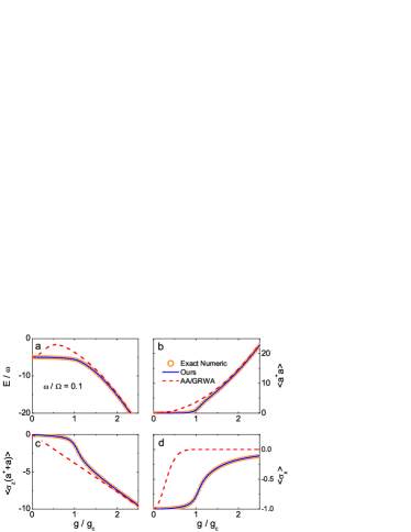
Figure 6: (Color online) Ground-state physical quantities as functions of the coupling strength $g/g_{c}$. $\omega/\Omega=0.1$ is taken as an example. a, The ground state energy. b, The mean photon number. c, The correlation function $\langle\sigma_{z}(a^{\dagger}+a)\rangle$. d, The tunneling strength $\langle\sigma_{x}\rangle$. The orange circles denote the numerically exact results as a benchmark, the red dashed-lines are calculated in adiabatic approximation(AA) Irish2005 or generalized rotating-wave approximation (GRWA) Irish2007 , and the blue lines are our results obtained by the present variational method.

The most widely-used approximations in the literature are the rotating-wave approximation (RWA)JC1963 , adiabatic approximation(AA) Irish2005 , generalized rotating-wave approximation (GRWA) Irish2007 and generalized variational method (GVM) GVM1 ; GVM2 , each working in some specific parameter regime. The RWA neglects the counter-rotating terms in the interaction, valid in regime $g\ll\omega,\Omega$ under near-resonance ($\omega\sim\Omega$) condition. The AA and the GRWA have the same groundstate, working for $g\gg\omega$ or negative detuning ($\omega>\Omega$) regime. The GVM works for $g\ll\omega$. Recently a mean-photon-number dependent variational method was proposed to cover validity regimes of both the GVM and the GRWA LiuM . However, all the approximations collapse when the ratio of $\omega/\Omega$ is getting small, e.g. below around $0.5$ (see Ref. [LiuM, ]). An improved variational method by including the antipolaronIrish2014 also finds breakdowns at $\omega/\Omega\sim 0.3$. It would be favorable to have a variational method that always preserves a high accuracy in varying all parameters which might facilitate and even deepen the physical analysis.

Indeed, our variational wavefunction yields such accuracy requirements. As an illustration, in Fig. 6 we compare with the exact numerics on the the ground state energy, mean photon number, coupling correlation and tunneling strength, at the example $\omega/\Omega=0.1$ (one can find other examples for comparison at $\omega/\Omega=0.01$, $0.05$, $0.15$, $0.5$ for another physical quantity $\gamma$ in Fig. 4 and Fig. 9). As a comparison, the results obtained by the AA or the GRWA are also shown. Clearly, our results are completely consistent with the exact ones in the whole parameter regime.

A.5 Physical necessity of the variational parameters

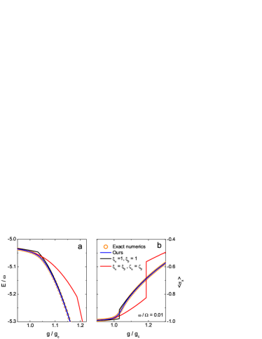
Figure 7: (Color online) Quantitative deviations and qualitative errors emerge in reducing variational parameters. Physical properties may deviate not only quantitatively but also qualitatively when the parameters are reduced, e.g., if imposing $\xi_{\alpha}=1,\ \xi_{\beta}=1$ (black line) or $\xi_{\alpha}=\xi_{\beta},\ \zeta_{\alpha}=\zeta_{\beta}$ (red line), an incorrect cusp behavior appears in the energy $E$ and the spin flipping (tunneling) strength $\langle\sigma_{x}\rangle$ has a spurious jump around $g_{c}$ at $\omega/\Omega=0.01$, in contradiction with the smooth crossover in the exact numerics (orange circles). The blue lines are our results in full minimal parameters which reproduce accurately the exact ones.

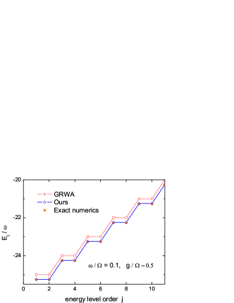
Figure 8: (Color online) An energy comparison of the excited states for the lowest 10 levels, at $\omega/\Omega=0.1$ and $g/\Omega=0.5$. The orange dots, empty blue diamonds and empty red squares represent the results of the exact numerics, our method and the GRWA, respectively.

It may be worthwhile to have further discussion on the physical necessity of the variational parameters. An unnecessary reduction of our parameters, on the one hand, will not lead to much of a reduction in the computational cost as the calculation in full parameters is actually quite easy to carry out, on the other hand, however, the price of physical loss would be too high. As discussed in the main part of the paper, our variational parameters physically correspond to the deformations of the polaron and the antipolaron with displacement and frequency renormalizations, which is justified by the behavior of the effective potential. In the subtle energy competitions of the potential of harmonic oscillator, the interaction and the tunneling, both the polaron and the antipolaron can adapt themselves via the variations of their displacements, frequencies and weights. Thus, corresponding to the key physical degree of freedom of the polaron and the antipolaron, the five variational parameters, $\xi_{\alpha},\ \xi_{\beta},\ \zeta_{\alpha},\ \zeta_{\beta},\alpha$, are the minimal necessary parameters to capture the true physics of the behavior of the polaron and the antipolaron, subject to the normalization of the wavefunction. Therefore, reducing the parameters would lead to mismatch of the physical degree of freedom and thus give rise to unreliable results, the physical properties may deviate not only quantitatively but also qualitatively. For an example, assuming $\xi_{\alpha}=\xi_{\beta}=1$ or imposing $\xi_{\alpha}=\xi_{\beta},\ \zeta_{\alpha}=\zeta_{\beta}$ can reduce the parameter number by 2. However, as shown in Fig.7, without mentioning the quantitative deviations, an incorrect cusp behavior appears in the energy $E$ at low frequencies as illustrated at $\omega/\Omega=0.01$, and even worse, a spurious jump emerges in the tunneling (spin flipping) strength $\langle\sigma_{x}\rangle$ around $g_{c}$. The other physical quantities, such as the mean photon number $\langle a^{\dagger}a\rangle$, the coupling correlation $\langle\sigma_{z}(a^{\dagger}+a)\rangle$ also have a false discontinuity similar to $\langle\sigma_{x}\rangle$. Both the cusp and the discontinuity are qualitatively in contradiction with the smooth crossover in the exact numerics (orange circles). Nevertheless, our results using the full minimal variational parameters (blue line) reproduce accurately the exact results in the entire regime of the coupling strengths at different frequencies. Moreover, in the cases of reduced parameters, some important underlying physics would also be missing, such as the scaling relation of the displacement and frequency renormalizations as we revealed in the main text (see also Appendix C).

A.6 Method extension to the excited states

Our method can also be useful for the excited states. As a first simple extension the variational energy of the excited state can be obtained by replacing expressions (14)-(16) with

$$h_{\alpha\alpha}^{+} = \frac{\omega}{2}\left[\left(n+\frac{1}{2}\right)\left(\xi_{\alpha}+\xi_{\alpha}^{-1}\right)+\left(1-\zeta_{\alpha}\right)^{2}g^{\prime 2}\right],$$ (31)

$$h_{\beta\beta}^{+} = \frac{\omega}{2}\left[\left(n+\frac{1}{2}\right)\left(\xi_{\beta}+\xi_{\beta}^{-1}\right)+\left(1-\zeta_{\beta}\right)^{2}g^{\prime 2}\right],$$ (32)

$$h_{\alpha\beta}^{+} = \frac{\omega}{2}\ \left[\left(1-\xi_{\alpha}^{2}\right)\left\langle\hat{x}_{\alpha}^{2}{}\right\rangle_{\alpha\beta}+\left(1-\zeta_{\alpha}\right)\left\langle\hat{x}_{\alpha}\right\rangle_{\alpha\beta}2g^{\prime}\right.$$ (33)

$$+\left.(2n+1)\xi_{\alpha}S_{\alpha\beta}+\left(1-\zeta_{\alpha}\right)^{2}g^{\prime 2}S_{\alpha\beta}\right],$$

where both $\langle\hat{x}_{\alpha}^{j}{}\rangle_{\alpha\beta}$ and $S_{\alpha\beta}$ can be included by a unified function

$$\langle\hat{x}_{\alpha}^{j}{}\rangle_{\alpha\beta}=X(n,j),\quad S_{\alpha\beta}=X(n,0).$$ (34)

Here the function $X(n,j)$ is defined by

$$X(n,j) = n!j!\left[\frac{\left(\zeta_{\alpha}+\zeta_{\beta}\right)g^{\prime}}{2c}\right]^{j}\sum_{p=0}^{\min[n,j]}\sum_{q=0}^{\min[n,j-p]}\frac{\left(-i\right)^{j-p-q}a^{p}b^{q}}{p!q!\left(j-p-q\right)!}\sqrt{\frac{2^{p+q}}{\left(n-p\right)!\left(n-q\right)!}}H_{j-p-q}\left(\frac{1}{2}ab^{2}c\right)\tilde{S}_{n-p,n-q},$$ (35)

$$\tilde{S}_{k,k^{\prime}} = \sum_{r=0}^{\min[k,k^{\prime}]}C_{kk^{\prime}r}H_{k-r}\left(\frac{ab^{2}c}{2\sqrt{1-a^{2}}}\right)H_{k^{\prime}-r}\left(-\frac{a^{2}bc}{2\sqrt{1-b^{2}}}\right),$$ (36)

$$C_{kk^{\prime}r} = \sqrt{\frac{ab}{2^{k+k^{\prime}}k!k^{\prime}!}}e^{-\left(abc\right)^{2}/4}\frac{k!k^{\prime}!\left(2ab\right)^{r}\left(1-a^{2}\right)^{(k-r)/2}\left(1-b^{2}\right)^{(k^{\prime}-r)/2}}{\left(k-r\right)!\left(k^{\prime}-r\right)!r!}.$$ (37)

and the factors $a,b,c$ depend on the variational parameters

$$a=\sqrt{\frac{2\xi_{\alpha}}{\xi_{\alpha}+\xi_{\beta}}},\quad b=\sqrt{\frac{2\xi_{\beta}}{\xi_{\alpha}+\xi_{\beta}}},\quad c=\left(\zeta_{\alpha}+\zeta_{\beta}\right)g^{\prime}\sqrt{\frac{\left(\xi_{\alpha}+\xi_{\beta}\right)}{2}}.$$ (38)

For the other group of overlap in the tunneling term $n_{+-}$(12), one can also formulate using $S_{\mu\bar{\mu}^{\prime}}=\left(-1\right)^{n}X(n,0)$ with the corresponding replacement $\alpha,\beta\rightarrow\mu,\mu^{\prime}$, but there is sign variation $\zeta_{\beta}\rightarrow-\zeta_{\mu^{\prime}}$. Here $n$ is the level number of the standard quantum harmonic oscillator and $H_{m}\left(x\right)$ is the standard Hermite polynomials. It is worthwhile to see that this simple extension for the excited states has already yielded some considerable improvements in strong couplings as illustrated in Fig.8 for a number of lowest energy levels. With the above expressions, one may further analytically construct an improved extension of the variational energy for overall coupling range by imposing the deformed polaron and antipolaron in the GRWA form of wavefunction. On the other hand, the dynamics of the system also can be calculated in terms of $\tilde{S}_{k,k^{\prime}}$ which provides the intra-overlap and inter-overlap of the deformed polarons and antipolarons with different oscillator quantum number $k,k^{\prime}$. Since here the focus is the ground state which, as we show in the present work, already has rich underlying physics to be uncovered, we shall present a more detailed method description and systematical discussion for the excited state properties in our future work.

Appendix B Quadpolaron/bipolaron changeover and scales of coupling strength

B.1 Analytic approximation for $g_{c}$

In the variation of the coupling strength, the system undergoes a phase-transition-like changeover around $g\sim g_{c}$. In the super-strong tunneling or low-frequency limit, i.e. $\omega/\Omega\rightarrow 0,$ this changeover is very sharp, it behaves more like a phase transition, as discussed by Ashhab Ashhab2013 . In the other cases it behaves like a crossover.

We can get more insights into this transition-like behavior from the profile deformation of the wavepacket. The increase of the coupling strength is splitting the wavepacket into the polaron and the antipolaron, while the tunneling is trying to keep them as close as possible in the groundstate. Before a full splitting the system remains in a quadpolaron state with four channels of tunneling, $S_{\alpha\bar{\alpha}}$, $S_{\beta\bar{\beta}}$, $S_{\alpha\bar{\beta}}$, and $S_{\beta\bar{\alpha}}$, while after the splitting the system enters a bipolaron state with only two tunneling channels, $S_{\alpha\bar{\beta}}$ and $S_{\beta\bar{\alpha}}$, surviving. Here we have labeled the tunneling channels by the overlaps $S_{i\bar{j}}$, defined in (13), to which the corresponding tunneling energies are proportional. We show the tunneling channel difference for these two regimes in Fig.9 a-c at various frequencies. One can also see that the change in the tunneling channel number is universal for different frequencies. Thus, the two regimes distinguished by wavepacket splitting are essentially different in the quantum states. Therefore, the coupling strength at which the splitting really starts can be used to formulate $g_{c}$.

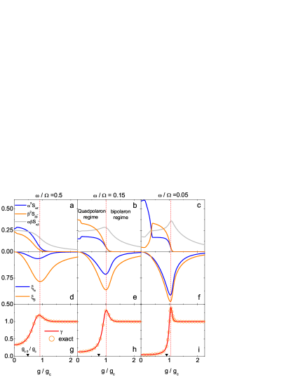
Figure 9: (Color online) Quadpolaron/bipolaron changeover and the behavior of variational parameters and related physical quantities. a-c, Weighted groundstate tunneling of different channels, $\alpha^{2}S_{\alpha\bar{\alpha}}$, $\beta^{2}S_{\beta\bar{\beta}}$, $\alpha\beta S_{\alpha\bar{\beta}}$ and $\alpha\beta S_{\beta\bar{\alpha}}$ ($S_{\beta\bar{\alpha}}=S_{\alpha\bar{\beta}}$) as functions of the coupling strength $g/g_{c}$. The dashed lines roughly separate the quadpolaron ($g\lesssim g_{c}$) regime and the bipolaron regime ($g\gtrsim g_{c}$), the former has four channels of tunnelings while the latter has two channels. d-f, The frequency renormalization factors $\xi_{\alpha}$ and $\xi_{\beta}$. g-i, The scaling quantity $\gamma$. The results from our variational method (solid lines) almost reproduce the ones from exact numerics (orange circles) for all values of coupling at different frequencies. The boundary of the quadpolaron and bipolaron regimes is associated with the minimum of $\xi_{i}$ and the maximum of $\gamma$. The black triangles mark the positions for $g_{c0}/g_{c}$ which becomes farther away from $1$ as $\omega$ increases. a,d $\omega/\Omega=0.5$. b, e, $\omega/\Omega=0.15$. c,f, $\omega/\Omega=0.05$.

We adopt the value of $g_{c}$ at the point where the distance between the polaron and the antipolaron is equal to their total radii,

$$\left(\zeta_{\alpha}+\zeta_{\beta}\right)g_{c}^{\prime}=r_{\alpha}+r_{\beta},$$ (39)

where we take the radii by

$$r_{\alpha}=2\sqrt{\frac{1}{\xi_{\alpha}}},\quad r_{\beta}=2\sqrt{\frac{1}{\xi_{\alpha}}},$$ (40)

at which the value of the corresponding wavepacket is becoming small

$$\frac{\varphi_{i}}{\varphi_{i}^{\max}}=\frac{1}{e^{2}}$$ (41)

for both $i=\alpha,\beta$.

Note that both sides of the above equation (39) are essentially averaging over the polaron and the antipolaron, thus assuming symmetric polaron and antipolaron, i.e. $\zeta_{\alpha}=\zeta_{\beta}$ and $\xi_{\alpha}=\xi_{\beta}$, would be a reasonable approximation as far as $g_{c}$ is concerned. Under this constraint the explicit results for the deformation parameters are available for the well-separated polaron and antipolaron from the energy minimization formulated in Appendix A, reading as

$$\zeta_{\alpha}=\zeta_{\beta}=\sqrt{1-\frac{g_{c0}^{4}}{g^{4}}},\quad\xi_{\alpha}=\xi_{\beta}=1,$$ (42)

where the critical point $g_{c0}=\sqrt{\omega\Omega}/2$ is obtained in the semiclassical approximation at $\omega/\Omega\rightarrow 0.$Ref-gc0 ; Ashhab2010 We stress that we limit the application of this approximation to the estimation of $g_{c}$, while for other properties one should fall back upon asymmetric polaron and antipolaron for higher accuracy. Actually, as mentioned in Appendix A, imposing symmetric polaron and antipolaron would lead to a spurious discontinuous behavior of physical properties, such as the tunneling strength, around $g_{c}$ at low frequencies, while in reality it should be smooth as predicted by asymmetric polaron and antipolaron in agreement with exact numerics. Also, in the strong coupling regime the displacement asymmetry of the polaron and the antipolaron actually plays an important role in inducing the amplitude-squeezing effect ($\xi_{\alpha}<1$) which extends the wavepackets of the polaron and the antipolaron to increase their overlap, thus enhancing the tunneling. Without the asymmetry there would be no squeezing beyond $g_{c}$, as indicated by (42), since the symmetric polaron and antipolaron in up and down spins would completely coincide, with an already-maximum overlap. In fact, as uncovered in the main text, there is a hidden relation between the squeezing and the displacement, which is also discussed in detail in Appendix C.

Substitution of (42) into (39) leads us to a simple analytic expression

$$g_{c}=\sqrt{\omega^{2}+\sqrt{\omega^{4}+g_{c0}^{4}}}.$$ (43)

It is easy to check $g_{c}\rightarrow g_{c0}$ in the slow oscillator limit $\omega/\Omega\rightarrow 0$. Besides the transition-like changeover in this low frequency limit, our $g_{c}$ is also providing a valid coupling scale for the quadpolaron/bipolaron changeover at finite frequencies, which can be seen from Fig.9 where the quadpolaron regime and bipolaron regime adjoin each other really around $g_{c}$. A more quantitative way to identify the transition-like point is, as shown by Fig.9 d-i, the minimum point of the frequency renormalization factor or the maximum point of the scaling quantity introduced in Appendix C. Still, one sees that it is well approximated by $g_{c}$ in (43).

B.2 Novel scale for the coupling strength

At this point, it is worthwhile to further discuss the scale of the coupling strength, the criterion for which is actually a bit controversial in the literatureIrish2014 . Although the terms for the coupling strengths were given in relation to the validity of the RWA as well as the progress of experimental accessibility, essentially the frequency $\omega$ has been conventionally taken as the evaluation scale: $g/\omega\leq 0.01$ for the weak coupling regime, $g/\omega\geq 0.01$ for the strong coupling, $g/\omega\geq 0.1$ for the ultrastrong coupling regimeNiemczyk2010 , $g/\omega\geq 1$ for deep strong coupling regimeCasanova2010 . On the other hand, it should be noticed that recently it has been proposed Irish2014 that the strength scale should be modified to be the semiclassical critical point $g_{c0}$. Still, as afore-mentioned, $g_{c0}$ is obtained in low-frequency semiclassical limit, while the situations at finite frequencies would be different. The controversy essentially comes from the fact that a consensus on the nature of the interaction-induced variation in different frequencies is still lacking. Here, our expression of $g_{c}$ in (43) is obtained by the observation that it is the wavepacket splitting that makes the essential change in increasing the coupling strength, which controls the final effective coupling tunneling strength and leads to transition (in low frequency limit) or crossover (at finite frequencies) of the quadpolaron/bipolaron states. We believe that $g_{c}$ is a more universal scale valid for all frequencies, as indicated by Fig. 9. Under these considerations, we simply divide the coupling strength into weak, intermediate and strong regimes under the conditions that $g$ is smaller than, comparable to and larger than $g_{c}$, respectively. As a reference, we compare the different scales for the coupling strength used in the literature in Fig.10.

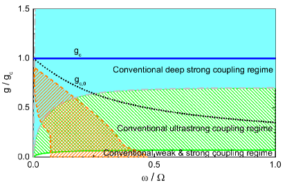
Figure 10: (Color online) The conventional coupling regimes used in the literature. The conventional ultrastrong coupling regime (the green shaded area) is enclosed by $g=0.1\omega$ and $g=\omega$, which has been reached by experiments in rapid progressNiemczyk2010 . The conventional deep strong coupling regime (the light-cyan area) is surrounded by $g=\omega$ and $g=10\omega$ (gray dash-dot lines), into which investigations have been enteringCasanova2010 . The black dotted line denotes the semiclassical critical-like point in low frequency limit, $g_{c0}$Ref-gc0 ; Ashhab2010 , proposed as a different scale of coupling strengthIrish2014 , while the blue solid line schematically represents the quadpolaron/bipolaron boundary $g_{c}$ as a novel scale generalized for the whole range of frequencies. Thus, the coupling strength is divided into weak, intermediate and strong regimes which correspond to that $g$ is smaller than, comparable to and larger than $g_{c}$, respectively. The orange-shaded window edged by the dash lines opens for the overweighted antipolaron discussed in our paper.

Appendix C Hidden scaling relation and symmetry-breaking-like aspect

C.1 Scaling relation extracted from energy minimization

When the coupling strength grows beyond $g_{c}$, we find that the squeezing factor $\xi_{i}$ and the displacement factor $\zeta_{i}$ begin to collapse into the same values and scale with each other in the further evolution, i.e.

$$\xi_{\alpha}\doteq\zeta_{\alpha},\quad\xi_{\beta}\doteq\zeta_{\beta}.$$ (44)

This hidden scaling relation can be more explicitly formulated at low frequencies. Note that the parameters can be extracted from the energy minimization

$$\frac{\delta E}{\delta\alpha}=0,\quad\frac{\delta E}{\delta\xi_{i}}=0,\quad\frac{\delta E}{\delta\zeta_{i}}=0.$$ (45)

In the bipolaron regime, only the polaron-antipolaron tunneling remains so the overlaps $S_{\alpha\bar{\alpha}}$ and $S_{\beta\bar{\beta}}$ are vanishing, but $S_{\beta\bar{\alpha}}$ is finite. In such a situation, controlling the polaron-antipolaron center of mass, $\zeta=\left(\zeta_{\alpha}+\zeta_{\beta}\right)/2$, can be decoupled from the relative motion in tunneling and squeezing, which enables us to extract the weight of the polaron,

$$\alpha=\sqrt{\frac{1+\zeta_{\beta}}{2-\left(\zeta_{\alpha}-\zeta_{\beta}\right)}}.$$ (46)

To obtain analytical results we assume a low frequency which enables a small-$\omega$ expansion and leads us to

$$\xi_{\alpha,\beta} = \xi\left(1\pm\frac{\omega^{2}}{4g^{2}}\right),$$

$$\zeta_{\alpha,\beta} = \zeta\left(1\pm\frac{\omega^{2}}{4g^{2}\left(1-g_{c0}^{4}/g^{4}\right)}\right),$$ (47)

where $\xi_{\alpha}$ ($\xi_{\beta}$) takes the sign $+$ ($-$). In the small-$\omega$ limit, $\xi_{i}$ and $\zeta_{i}$ collapse into their average $\xi=\left(\xi_{\alpha}+\xi_{\beta}\right)/2$ and $\zeta=\left(\zeta_{\alpha}+\zeta_{\beta}\right)/2$ which are equal:

$$\xi=\zeta=\sqrt{1-\frac{g_{c0}^{4}}{g^{4}}},$$ (48)

up to $\omega^{2}$ order. We can see the scaling relation from the approximate analytic results: (i) in low-frequency limit, one sees that $\xi_{i}\doteq\zeta_{i}$ holds, up to an $\omega^{2}$ order correction which is negligible for small $\omega$. (ii) For higher frequencies, the $\omega^{2}$ terms in $\xi_{\alpha,\beta}$ and $\zeta_{\alpha,\beta}$ become almost the same due to $g_{c0}^{4}/g^{4}\ll 1$, since in bipolaron regime we have $g>g_{c}>g_{c0}$ (e.g., for $\omega=0.5\Omega$, $g_{c0}^{4}/g_{c}^{4}=0.056$ while $g_{c0}^{4}/g^{4}$ is negligible beyond the crossover range.). These analytic considerations account for the scaling relation as we showed in the main text for different frequencies.

To test the scaling relation, we shall propose a physical quantity that may be either measured experimentally or verified by exact numerics. On one hand, applying the above expansion to the photon number (22) and neglecting the difference of $\xi_{\alpha},\zeta_{\alpha}$ and $\xi_{\beta},\zeta_{\beta}$ leads us to an expression of $\zeta$ as a function of $\langle a^{+}a\rangle$ and $\xi$

$$\zeta\doteq\frac{\omega}{g}\sqrt{\langle a^{+}a\rangle-\frac{1}{4}(\xi+\xi^{-1})+\frac{1}{2}}.$$ (49)

On the other hand, the same approximation yields

$$\xi\doteq-\langle\left(a^{+}-a\right)^{2}\rangle.$$ (50)

Thus, considering the ratio $\zeta/\xi$, we introduce the following phyiscal quantity

$$\gamma\equiv\frac{\omega}{gt}\sqrt{\langle a^{+}a\rangle-\frac{1}{4}(t+t^{-1})+\frac{1}{2}},$$ (51)

where we have defined $t=-\langle\left(a^{+}-a\right)^{2}\rangle$. In the bipolaron regime with strong couplings, this quantity becomes the scaling ratio, $\gamma\rightarrow\zeta/\xi$. In this regime, if the scaling relation (44) holds, the value of $\gamma$ will be equal to 1. Indeed, this scaling relation is confirmed by the exact numerics, as shown in the main text.

In the quadpolaron regime with intermediate or weak couplings, not only the scaling relation (44) is violated but also the relation between $\gamma$ and $\zeta/\xi$ is breaking down, $\gamma\neq\zeta/\xi$. Nevertheless, we find that, besides the bipolaron regime having the value $\gamma=1$, the quadpolaron with four strong channels of tunneling is located in the range $\gamma<1$ and the state with decaying left-right tunnelings ($S_{\alpha\bar{\alpha}}$, $S_{\beta\bar{\beta}}$) falls in a range $\gamma>1$, as one can see in Fig.9a-c,g-i. In this sense, according to the values and behavior of $\gamma$, one can distinguish the quantum states of the bipolaron, quadpolaron and their changeover, respectively.

C.2 Scaling relation alternatively obtained from the lowest-order expansion of the effective potential

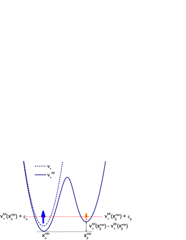
Figure 11: (Color online) Spin-up single-particle effective potential, $v_{+}^{tot}=v_{+}+\delta v_{+}$, in the strong coupling regime. As in this regime within the same spin component there is no overlap between the polaron ($\alpha$, labelled by the blue arrow) and antipolaron ($\beta$, labelled by the orange arrow) in the two wells, to have both finite weights for the polaron and the antipolaron the two sub-well energies have to be degenerate, i.e., $v_{+}^{tot}(x^{min}_{\alpha})+\varepsilon_{\alpha}=v_{+}^{tot}(x^{min}_{\beta})+\varepsilon_{\beta}$. Here $x^{min}_{i}$ is the position of local minimum potential and $\varepsilon_{i}=\xi_{i}$ (scaled by $\omega/2$), $i=\alpha,\beta$.

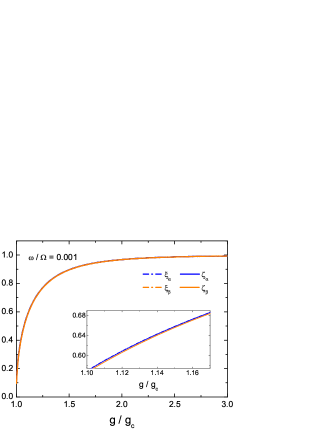
Figure 12: (Color online) Scaling relation alternatively obtained from the expansion of $v_{+}^{tot}$. $\omega/\Omega=0.001$ is taken. $\xi_{i}$ and $\zeta_{i}$ almost take the same values in the strong coupling regime above the $g_{c}$. The inset shows their tiny differences by a zoom-in plot.

Apart from variational method on energy minimization introduced in Appendix A, an alternative way to see the scaling relation is to investigate the effective potential. As we discussed in the main text, the eigenequation actually can be written in a single particle form

$$\frac{1}{2}\omega\left(\hat{p}^{2}+v_{\pm}^{tot}\right)\psi_{\pm}=E\psi_{\pm},$$ (52)

where we have assumed that the particle mass $m=1$ and the total potential is composed of the bare potential $v_{\pm}$ and an additional effective potential $\delta v_{\pm}$ induced by the tunneling,

$$v_{\pm}^{tot}=v_{\pm}+\delta v_{\pm},$$ (53)

with

$$v_{\pm}=\left(x\pm g^{\prime}\right)^{2},\quad\delta v_{\pm}=\eta\frac{\Omega}{\omega}\frac{\psi_{\mp}}{\psi_{\pm}},$$ (54)

and we have considered the ground state with $\eta=-1$. In the strong coupling regime, the total potential exhibits an obvious two-well structure, with a larger barrier separating the wells, as shown in Fig. 11.

In the lowest order, the two wells can be considered as a local harmonic potential. Actually, an expansion around the local minimum point $x_{i}^{\min}$ of the potential leads to

$$v_{+}^{tot}\cong v_{+}^{tot}(x_{i}^{\min})+f_{i}^{(1)}\left(x-x_{i}^{\min}\right)+f_{i}^{(2)}\left(x-x_{i}^{\min}\right)^{2},$$ (55)

where $x_{i}^{\min}=\eta_{i}\zeta_{i}g^{\prime}$ with $i=\alpha,\beta$, and $\eta_{\alpha}=-1$, $\eta_{\beta}=1$ respectively for the polaron and the antipolaron. The coefficients are defined by

$$f_{i}^{(1)}=\frac{\partial v_{+}^{tot}}{\partial x}|_{x=x_{i}^{\min}},\quad f_{i}^{(2)}=\frac{1}{2}\frac{\partial^{2}v_{+}^{tot}}{\partial x^{2}}|_{x=x_{i}^{\min}}.$$ (56)

First, the approximation of local harmonic potential requires

condition-1: $$\quad f_{i}^{(1)}=0,$$ (57)

condition-2: $$\quad f_{i}^{(2)}=\xi_{i}^{2}.$$ (58)

The condition-1 ensures the potential minimum point at $x_{i}^{min}$, while the condition-2 indicates the same renormalized frequency $\xi_{i}\omega$ of the local harmonic potential as that of the wavefunction of the harmonic oscillator. Furthermore, since effectively there is no single-particle inter-site hopping (if regarding the wells as two sites) in the presence of the large barrier in the strong coupling regime, to have finite weights for both the polaron and the antipolaron in the single-particle effective potential the local energies of the two wells need to be degenerate

$$\text{condition-3:\quad}v_{+}^{tot}(x_{\alpha}^{\min})+\varepsilon_{\alpha}=v_{+}^{tot}(x_{\beta}^{\min})+\varepsilon_{\beta},$$ (59)

where

$$\varepsilon_{i}=\xi_{i}$$ (60)

is the energy of the local harmonic oscillator scaled by $\omega/2$ and

$$v_{+}^{tot}(x_{i}^{\min})=v_{+}(x_{i}^{\min})+\delta v_{+}(x_{i}^{\min})$$ (61)

corresponds to the reference energy. Taking the variational wavefunction (6), in the strong coupling regime we have

$$\delta v_{+}(x_{\alpha}^{\min})\doteq-\frac{\Omega}{\omega}\frac{\beta\varphi_{\beta}(-x_{\alpha}^{\min})}{\alpha\varphi_{\alpha}(x_{\alpha}^{\min})},$$

$$\delta v_{+}(x_{\beta}^{\min})\doteq-\frac{\Omega}{\omega}\frac{\alpha\varphi_{\alpha}(-x_{\beta}^{\min})}{\beta\varphi_{\beta}(x_{\beta}^{\min})}.$$ (62)

while $\beta=\sqrt{1-\alpha^{2}}$ in the strong coupling regime.

Now one can (i) control the displacement renormalization $\zeta_{i}$ to satisfy condition-1 so that the linear term $f_{i}^{(1)}$ is eliminated and the minimum is located at $x_{i}^{\min}$, (ii) tune the frequency renormalization $\xi_{i}$ to fulfill condition-2 so that both the local potential and the wavefunction self-consistently shares the same frequency $\xi_{i}\omega$, (iii) balance the weight ratio of $\alpha/\beta$ to meet condition-3 so that the two wells have degenerate local energies to self-consistently guarantee the finiteness of the weights $\alpha$ and $\beta$. At this point, we see that the degree of the basic deformation factors introduced for our variational wavefunction is consistent with the minimum requirements of self-consistence conditions.

From Conditions-1,2,3 we also refind the scaling relation as illustrated by Fig.12, which might provide some alternative insights for the scaling relation that we obtained from the energy minimization in last subsection. Still, we should mention there is a small difference between the two ways, since the above consideration from the effective potential is based on the lowest order expansion which guarantees only the local potential itself to be harmonic without taking care of the energy, while the energy minimization ensures only the most favorable energy but the effective potential $\delta v_{\pm}=\eta\frac{\Omega}{\omega}\frac{\psi_{\mp}}{\psi_{\pm}}$ includes higher order terms beyond the harmonic potential approximation. Despite the small difference, both approaches lead to the scaling relation.

C.3 Symmetry-breaking-like aspect for the bipolaron-quadpolaron quantum state changeover

With the scaling relation at hand, it might provide some more insight to discuss the quantum state changeover from the symmetry point of view. Generally, for all eigenstates, the Hamiltonian has the parity symmetry, ${\cal P}=\sigma_{x}(-1)^{a^{+}a}$ which involves simultaneous reversion of the spin and the space. Specifically for the ground state that we are focusing on in this work, one could find extra symmetries. In fact, in the low frequency limit the photon number vanishes for the ground state below $g_{c}$, as indicated by Fig.6b (this is more obvious for lower frequencies), so that additionally the total parity symmetry can be decomposed into separate spin reversal symmetry $\sigma_{x}$ and oscillator spatial reversal symmetry $(-1)^{a^{+}a}$. These additional symmetries are broken beyond $g_{c}$ due to the emergence of a number of photons, so that there is a subsymmetry transition when the system goes across $g_{c}$. Still, these spin and spatial subsymmetries are considered from the weak coupling side and become less valid at finite frequencies due to a nonvanishing photon number. Nevertheless, our finding of the scaling relation provides compensation but from the strong coupling side. Actually, as shown in Fig.4, the physical quantity we proposed, $\gamma$, demonstrates an invariant behavior beyond $g_{c}$, which confirms the scaling relation and thus the symmetric aspect between the displacement and frequency renormalizations in this regime. Note that, as shown in last subSection, in this bipolaron regime the remaining left-left and right-right tunnelings (i.e. polaron-antipolaron inter-tunnelings) render both the polaron and the antipolaron to have finite weights, while to preserve finite weights as a quantum effect in the absence of left-right tunneling channels (i.e. intra-polaron and intra-antipolaron tunnelings) the polaron and the antipolaron have to maintain the displacement-frequency scaling relation. In other words, this displacement-frequency symmetry arises only in the absence of the left-right channels, and conversely, there will be no left-right channels if the symmetry is preserved there. Going from the bipolaron regime to the quadpolaron regime, this symmetry will be broken in the presence of the left-right tunneling channels. In this sense, besides the afore-mentioned parity subsymmetry breaking originating from the weak coupling side in the low frequency limit, for both low frequency limit and finite frequencies there is another hidden symmetry-breaking-like behavior in the changeover of the two quantum states stemming from the strong coupling side. Thus, it is interesting to see a deeper nature of the interaction that not only induces the bipolaron/quadpolaron quantum state changeover but also brings about the symmetry breaking.

Appendix D Physical implications and method extension to the multiple-mode case

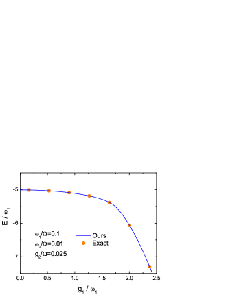
Figure 13: (Color online) Ground-state energy as a function of $g_{1}$ in the two-mode case. The parameters used are $\omega_{1}/\Omega=0.1,\omega_{2}/\Omega=0.01$ and $g_{2}/\Omega=0.025$. Our variational method (solid line) is in good agreement with exact numerics(dots).

D.1 Physical implications for the spin-boson model

Our ground-state phase diagram obtained for the Rabi model might also provide some insights or implications for the spin-boson model Spin-Boson which is a multiple-mode version of the Rabi model and has wide relevance to other fields, including the Kondo model RelevanceKondo and the Ising spin chain RelevanceIsing in condensed matter.

On the one hand, the bipolaron/quadpolaron changeover in the Rabi model can provide insights for localized/delocalized transition in the spin-boson model. In fact, the spin-boson model exhibits different behaviors in the Ohmic, super-Ohmic, and sub-Ohmic spectra, which actually have different weights of distributions for low and high frequency modes. Note that, as discussed in our work on the nature of the interaction-induced variation, the bipolaron and the quadpolaron states respectively have blockaded and enhanced left-right tunnelings, which is closely related to the situation of the localized and delocalized states involved in the spin-boson model. As indicated by our ground-state phase diagram and the obtained $g_{c}$ expression, the same coupling could be located in different regimes depending on whether frequency is low or high. Our ground-state phase diagram and $g_{c}$ expression might provide a primary reference and some insights into the different behaviours of the Ohmic, super-Ohmic, and sub-Ohmic spectra, since the distribution weights of low and high frequencies would make different contributions to blockaded and enhanced tunneling, thus affecting the competition in the quantum phase transition of the localized and delocalized states.

On the other hand, the overweighted antipolaron region might have some implication for the coherence-incoherence transition in the spin-boson model. It has been found that, within the delocalized phase of the spin-boson model, there is possibly another coherence-incoherence transition Tong2011 ; Spin-Boson for which the nature is still not very clear. Interestingly, in our ground-state phase diagram of the Rabi model, within the strong-tunneling regime in the quadpolaron state, there is also an underlying particular region characterized by an unexpected overweighted antipolaron, the possible implication and relation of the overweighted antipolaron regime in the Rabi model and the coherence-incoherence transition in the spin-boson model might be worthwhile exploring.

Since in the present work our focus is on the single-mode Rabi model, we would like to leave the investigations of these possible implications for the spin-boson model to some future works. Nevertheless, in the following we provide some indication of the method and variational wavefunction.

D.2 Method extension to the multiple-mode case

The basic variational physical ingredients introduced in the single-mode case also should apply for the multiple-mode case. The treatments are readily extendable from the single-mode case. The Hamiltonian including $M$ modes of harmonic oscillators can be written as

$$H=\sum_{k=1}^{M}\omega_{k}a_{k}^{\dagger}a_{k}+\sigma_{z}\sum_{k=1}^{M}g_{k}(a_{k}^{\dagger}+a_{k})+\frac{\Omega}{2}\sigma_{x}.$$ (63)

We propose the variational trial wavefunction as

$$\psi[\{x_{k}\}]=\alpha\prod_{k=1}^{M}\varphi_{\alpha}^{k}+\beta\prod_{k=1}^{M}\varphi_{\beta}^{k},$$ (64)

where $\varphi_{\alpha}^{k}$ ($\varphi_{\beta}^{k}$) is the $k$’th mode polaron (antipolaron) under the direct extension $\{\omega,g,x,\xi_{i},\zeta_{i}\}\rightarrow\{\omega_{k},g_{k},x_{k},\xi_{i}^{k},\zeta_{i}^{k}\}$. The energy is simply that of the single-mode energy in (10) with the overlap integrals replaced by the product of all modes. We find the same accuracy as in the single-mode case, as illustrated in Fig.13 by an example of the two-mode case, for which exact numerics are available for comparison. One can also include a bias term $\epsilon\sigma_{z}$ with a broken parity for $\psi_{\sigma}\left(x\right)$ at different spin $\sigma$. The multiple-mode case deserves special investigations in detail which we shall discuss in future works.

References

- (1) A. Wallraff et al., Nature 431, 162 (2004).
- (2) G. Günter et al., Nature 458, 178 (2009).
- (3) T. Niemczyk et al., Nature Phys. 6, 772 (2010).
- (4) B. Peropadre, P. Forn-Díaz, E. Solano, and J. J. García-Ripoll, Phys. Rev. Lett. 105, 023601 (2010).
- (5) P. Forn-Díaz et al., Phys. Rev. Lett. 105, 237001 (2010).
- (6) P. Cristofolini et al., Science 336, 704 (2012).
- (7) G. Scalari et al., Science 335, 1323 (2012).
- (8) Z.-L. Xiang, S. Ashhab, J. Q. You, and F. Nori, Rev. Mod. Phys. 85, 623 (2013).
- (9) C. Ciuti and I. Carusotto, Phys. Rev. A 74, 033811 (2006).
- (10) M. Devoret, S. Girvin, and R. Schoelkopf, Ann. Phys. 16, 767 (2007).
- (11) E.T. Jaynes and F. W. Cummings, Proc. IEEE 51, 89 (1963).
- (12) L. Allen and J. H. Eberly, Optical Resonance and Two-Level Atoms (Dover Publications, New York, 1987).
- (13) I. I. Rabi, Phys. Rev. 49, 324 (1936).
- (14) I. I. Rabi, Phys. Rev. 51, 652 (1937).
- (15) C. Cohen-Tannoudji, J. Dupont-Roc, and G. Grynberg, Atom-Photon Interactions: Basic Processes and Applications (John Wiley & Sons, New York, 1992).
- (16) C. Ciuti, G. Bastard, and I. Carusotto, Phys. Rev. B 72, 115303 (2005).
- (17) J. Bourassa et al., Phys. Rev. A 80, 032109 (2009).
- (18) J. Casanova, G. Romero, I. Lizuain, J. J. García-Ripoll, and E. Eolano, Phys. Rev. Lett. 105, 263603 (2010).
- (19) E. K. Irish and J. Gea-Banacloche, Phys. Rev. B 89, 085421 (2014).
- (20) D. Braak, Phys. Rev. Lett. 107, 100401 (2011).
- (21) E. Solano, Physics 4, 68 (2011).
- (22) Q.-H. Chen, C. Wang, S. He, T. Liu, and K.-L. Wang, Phys. Rev. A 86, 023822 (2012).
- (23) F. Alexander Wolf, M. Kollar, and D. Braak, Phys. Rev. A 85, 053817 (2012).
- (24) S. Bera et al., Phys. Rev. B 89, 121108(R) (2014).
- (25) S. Bera, A. Nazir, A. W. Chin, H. U. Baranger, and S. Florens, Phys. Rev. B 90, 075110 (2014).
- (26) A. J. Leggett, S. Chakravarty, A. T. Dorsey, M. P. A. Fisher, A. Garg, and W. Zwerger, Rev. Mod. Phys. 59, 1 (1987).
- (27) H. Walther, B. T. H. Varcoe, B. Englert and T. Becker, Rep. Prog. Phys. 69, 1325 (2006).
- (28) J. M. Raimond, M. Brune, and S. Haroche, Rev. Mod. Phys. 73, 565 (2001).
- (29) T. Holstein, Ann. Phys. 8, 325 (1959).
- (30) G. D. Mahan, Many-Particle Physics 3th Ed. (Kluwer Academic/Plenum Publishers, New York, 2000).
- (31) S. Ashhab and F. Nori, Phys. Rev. A 81, 042311 (2010).
- (32) J. Restrepo, C. Ciuti, and I. Favero, Phys. Rev. Lett. 112, 013601 (2014).
- (33) P. Meystre, Annalen der Physik 525, 215 (2013).
- (34) E. K. Irish, J. Gea-Banacloche, I. Martin, and K. C. Schwab, Phys. Rev. B 72, 195410 (2005).
- (35) E. K. Irish, Phys. Rev. Lett. 99, 173601 (2007).
- (36) Y. Zhang, G. Chen, L. Yu, Q. Liang, J.-Q. Liang, and S. Jia, Phys. Rev. A 83, 065802 (2011).
- (37) L. Yu, S. Zhu, Q. Liang, G. Chen, and S. Jia, Phys. Rev. A 86, 015803 (2012).
- (38) M. Liu, Z.-J. Ying, J.-H. An, and H.-G. Luo, New J. Phys. 17, 043001 (2015).
- (39) S. Ashhab, Phys. Rev. A 87, 013826 (2013).
- (40) R. Graham and Höhnerbach, Zeitschrift für Phys. B Condens. Matter 57, 233 (1984).
- (41) F. Guinea, V. Hakim, and A. Muramatsu, Phys. Rev. B 32, 4410 (1985).
- (42) A. Winter, H. Rieger, M. Vojta, and R. Bulla, Phys. Rev. Lett. 102, 030601 (2009).
- (43) Q.-J. Tong, J.-H. An, H.-G. Luo, and C. H. Oh, Phys. Rev. B 84, 174301 (2011).