DPF2015-49

Signal Processing in the MicroBooNE LArTPC

Jyoti Joshi, Xin Qian
(For THE MicroBooNE Collaboration)

Department of Physics
Brookhaven National Laboratory, Upton, NY 11973, USA

The MicroBooNE experiment is designed to observe interactions of neutrinos with a Liquid Argon Time Projection Chamber (LArTPC) detector from the on-axis Booster Neutrino Beam (BNB) and off-axis Neutrinos at the Main Injector (NuMI) beam at Fermi National Accelerator Laboratory. The detector consists of a $2.5~{}m\times 2.3~{}m\times 10.4~{}m$ TPC including an array of 32 PMTs used for triggering and timing purposes. The TPC is housed in an evacuable and foam insulated cryostat vessel. It has a 2.5 m drift length in a uniform field up to 500 V/cm. There are 3 readout wire planes (U, V and Y co-ordinates) with a 3-mm wire pitch for a total of 8,256 signal channels. The fiducial mass of the detector is 60 metric tons of LAr.

In a LArTPC, ionization electrons from a charged particle track drift along the electric field lines to the detection wire planes inducing bipolar signals on the U and V (induction) planes, and a unipolar signal collected on the (collection) Y plane. The raw wire signals are processed by specialized low-noise front-end readout electronics immersed in LAr which shape and amplify the signal. Further signal processing and digitization is carried out by warm electronics. We present the techniques by which the observed final digitized waveforms, which comprise the original ionization signal convoluted with detector field response and electronics response as well as noise, are processed to recover the original ionization signal in charge and time. The correct modeling of these ingredients is critical for further event reconstruction in LArTPCs.

PRESENTED AT

DPF 2015
The Meeting of the American Physical Society
Division of Particles and Fields
Ann Arbor, Michigan, August 4–8, 2015

1 Liquid Argon Time Projection Chambers

Liquid Argon Time Projection Chambers (LArTPCs) [1, 2] provide a powerful, robust, and elegant solution for studying neutrino interactions and probing the parameters that characterize neutrino oscillations. LArTPC technology offers a unique combination of millimeter scale 3D precision particle tracking and calorimetry with good dE/dx resolution. This combination results in high efficiencies for particle identification and the background rejection. Due to its scalability and fine grained tracking capability, LArTPC technology is a promising choice for the next generation massive neutrino detectors. Liquid Argon is an ideal medium since it has high density, excellent properties such as large ionization and scintillation yields, is intrinsically safe and cheap, and is readily available anywhere as a standard by-product of the liquefaction of air. The operating principle of large scale LArTPC detectors is based on the fact that in highly purified liquid argon, ionization tracks can be transported by a uniform electric field over distances of the order of meters.

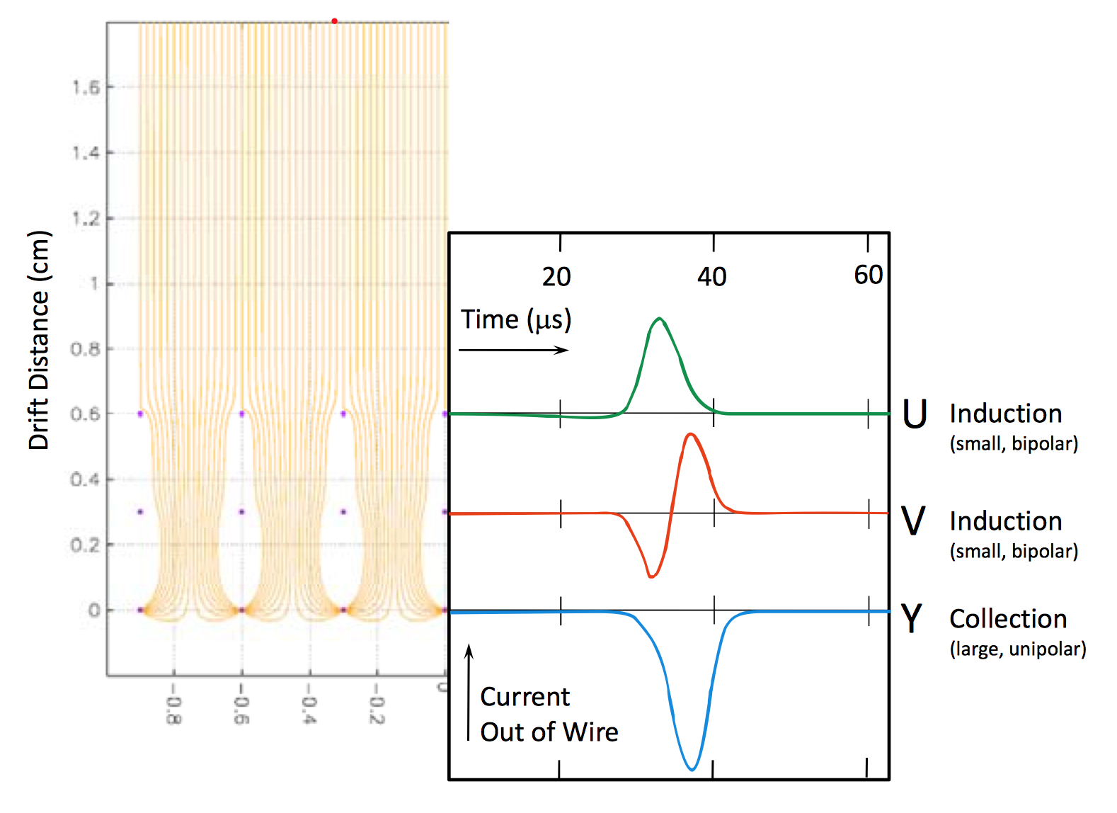
Figure 1: The signal properties of LArTPC

A single-phase LArTPC is basically a tracking wire chamber placed in highly purified liquid argon with an electric field created within the detector. Ionization electrons produced when charged particles go through the detector volume would drift along the electric field until they reach the wire-planes and hence produce signals that are utilized for imaging purposes. Several wire-planes with different orientations using bias voltages chosen for optimal field shaping give several complimentary views of the same interaction as a function of drift time, providing the necessary information for reconstructing a three-dimensional image of the interaction [3].

A schematic illustrating the LArTPC signal response is shown in Fig. 1. It shows the planar illustration of electric field lines (i.e, electron trajectories) and the signals induced by an ionizing track at $90\degree$ to the wire direction and at $0\degree$ to the wire planes. In the simulation, the wires in the induction planes U and Y are inclined at $\pm 45\degree$ with respect to wires in the Y collection plane. Bipolar signals from two induction planes, and the unipolar signal from the collection plane are processed and readout by specialized low-noise front-end readout electronics immersed in LAr.

2 The MicroBooNE LArTPC

MicroBooNE [4, 5] is newly built LArTPC neutrino detector of 60 metric ton fiducial mass (170 ton total) at Fermilab National Accelerator Laboratory in Batavia, Illinois. MicroBooNE recently started its operation and has been collecting neutrino data from the Booster Neutrino Beamline (BNB) since October, 2015. The experiment’s primary motivation is to resolve the source of the MiniBooNE low energy excess observed in $\nu_{e}$ candidates by taking advantage of the excellent electron-photon particle identification capabilities of a LArTPC in addition to carrying out a comprehensive suite of neutrino cross section measurements on Argon.

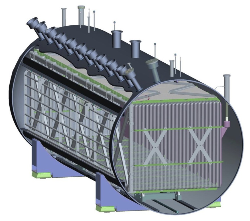
Figure 2: Schematic diagram of MicroBooNE detector

The TPC itself contains three wire planes, one collection plane at $0\degree$ from vertical and two induction planes at $\pm 60\degree$ with 3-mm wire pitch and 3-mm wire plane separation. MicroBooNE also serves as a test bed for LArTPC technologies for next generation very large scale detectors. There are many innovative technologies implemented, such as 2.5 m long drift distance, cold front-end low-noise readout electronics [6] and a filling procedure that does not include prior evacuation of the cryostat while still maintaining ultra-high purity LAr. The use of cold electronics within the LAr volume is critical for enabling the scaling up of the LArTPC technology and to improve the signal-to-noise ratio. The light collection system [7] consists of 32 8-inch PMTs that are located just behind the wire planes to detect scintillation light from $\nu$-Ar interactions. The PMT information is used to trigger on beam events and significantly reduce the data throughput. A schematic diagram of the MicroBooNE detector is shown in Fig. 2.

3 Signal Processing Chain

The raw signal on the wires in the TPC consists of both the ionization signal and the noise. The signal is a convolution of the distribution of the electron cloud passing through the TPC wires, the field response (i.e. the induced current on wires), and the electronics response. The background includes the noise from various sources. The goal of signal processing is to extract both the signal charge and time information reliably and separate it from the noise. The following subsections will give details on each step.

3.1 Field and Electronics Response Modeling

A detailed knowledge of the field and electronics response is necessary in order to characterize the detector performance. Simulating the field response function is the first step in the chain of signal processing. The drifting electrons are modeled as many small clouds of charge that diffuse as they travel toward the collection wires. The response of the channels to the drifting electrons is parameterized as a function of drift time, with separate response functions for collection and induction wires. The signals on the induction-plane wires result from induced currents and are thus bipolar as a function of time as charge drifts past the wires, while the signals on the collection plane wires are unipolar. Fig. 3 (left) shows the 2-D GARFIELD [8] simulated response to a single electron blob generated in the MicroBooNE detector geometry in terms of charge vs. time averaged for a single electron for both induction planes (U-Plane in black and V-Plane in red) and collection plane (in blue).

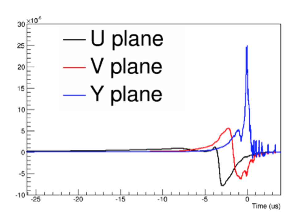
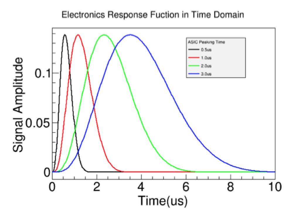
Figure 3: Field Response Functions (left) and Electronics Shaping Functions (right)

The electronics response function for the MicroBooNE detector is shown in Fig. 3 (right) in terms of signal amplitude vs. time. Since the MicroBooNE front-end cold electronics are designed to be programmable with 4 different gain settings (4.7, 7.8, 14, and 25 mV/fC) and 4 shaping time settings (0.5, 1, 2, and 3 us), the electronic response function varies according to these settings. Different colored lines in Fig. 3 (right) show the electronics response for different shaping time settings. For a fixed gain setting, the peak is always at the same height independent of the shaping time.

3.2 Raw and Convoluted Signal

In this section the true raw wire signal and the actual signal obtained after processing by the readout electronics are described. The digitized signal obtained after the ADC is formed when the ionization signal is convoluted with the detector and the front-end cold electronics response functions and then digitized at a fixed frequency. The top row of Fig. 4 shows the raw MIP signal in the U, V and Y-Planes and in the bottom row, the raw signal convoluted with field and electronics response for different shaping time settings are shown.

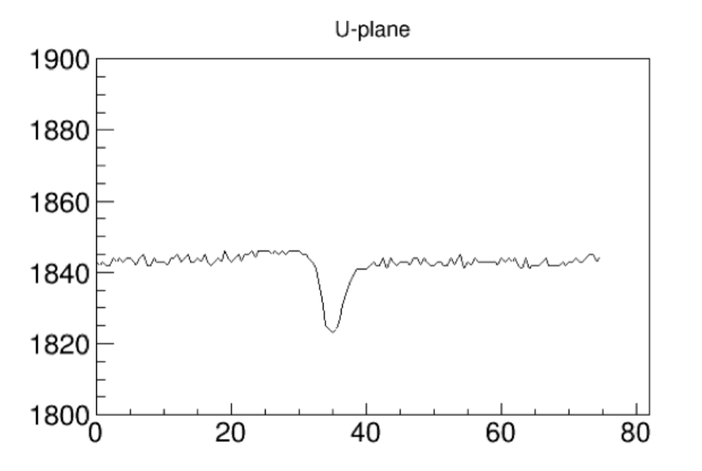
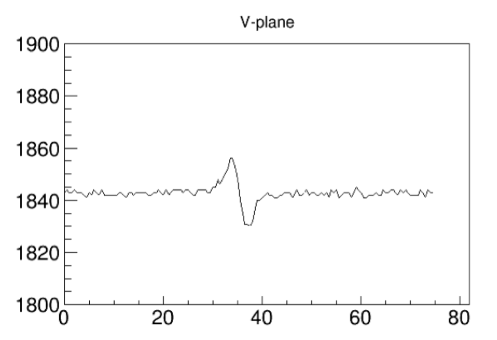
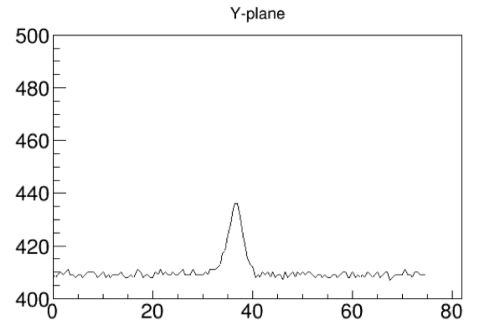
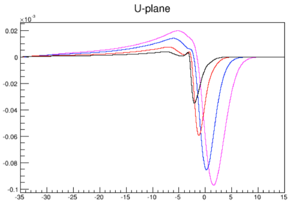
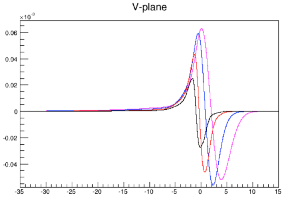
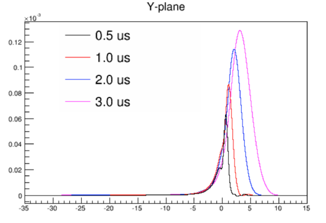
Figure 4: Raw Signal (top row); Convoluted Signal (bottom row) for U, V and Y-Plane respectively

3.3 Noise Sources in Detector

The readout electronics and digitization circuits are the two main sources of noise in the detector. In the case of the front-end readout electronics, the first transistor noise is the main component [6]. The first transistor noise contribution to the measured signal charge is proportional to the total capacitive load on the input channel, comprised of the sense wire capacitance, cable capacitance, and input transistor capacitance. This total capacitance limits the signal-to-noise ratio and it is the one dominant factor on which the feasibility and scalability of a LArTPC design critically depends. The other electronics noise sources are from thermal noise on the sense wires and connection leads (signal cable). Usually, thermal noise is made negligible by choosing appropriate resistors. Digitization noise arises during the signal digitization by the ADC which has a 12-bit resolution and a sampling rate of 2 mega-samples per second (MS/s). The digitizer has been chosen in such a way to ensure that digitization noise is much smaller than the front-end electronics noise.

Other noise sources such as microphonics, and pick-up noise on the TPC wires could also be present in the detector. These can be eliminated using further signal processing steps that are not discussed in this report.

3.4 Deconvolution

The next stage of signal processing is termed “Deconvolution”, which means reversing the effects of convolution by unpacking and removing the readout electronics and field response of the wire planes. The basic deconvolution process is implemented in the standard LArSoft [9] software signal processing procedure which was originally developed by the ArgoNeuT experiment [10], and further developed by MicroBooNE. The process of deconvolution is explained using the following equations.

$$M(t_{0})=\int_{\{t\}}R(t-t_{0}).\,S(t)\,dt$$ (1)

$$M(w)=R(w).S(w)$$ (2)

$$S(w)=\frac{M(w)}{R(w)}$$ (3)

If M is the measured signal i.e, the digitized signal convoluted with the response functions R, and S is the desired real signal, then the measured signal in the time domain is given by Eq. (1). In order to remove the effects of the different response functions, a fast fourier transformation (FFT) [11] is performed on the measured signal in the time domain. The resulting measured signal in the frequency domain is as shown in Eq. (2). By using simple factorization, the real deconvoluted signal (number of electrons reaching wire planes) is then extracted in the frequency domain, Eq. (3). To obtain the real charge signal in time domain S(t), an inverse fourier transformation is performed.

As discussed in the previous section, there are different types of noise sources present in the detector and in order to extract the true charge signal from the measured signal, the noise contribution to the measured signal needs to be eliminated as much as possible. The filtering of the noise from the measured signal will be discussed in next section.

3.5 Noise Filtering

To remove noise from the deconvoluted signal, a Wiener noise filter  [12] is constructed using the expected signal and noise frequency response functions. The Wiener filter can be defined as in Eq. (4), where S is the signal and N is the noise in the frequency domain.

$$F(w)=\frac{S^{2}(w)}{S^{2}(w)+N^{2}(w)}$$ (4)

Wiener deconvolution is done in the frequency domain in order to minimize the impact of deconvolved noise at frequencies which have a poor signal-to-noise ratio. Using the noise filter, $F(w)$, in the deconvolution method, Eq. (3) is modified as such:

$$S(w)=\frac{M(w)}{R(w)}.F(w)$$ (5)

The effect of noise and the process of noise filtering is described in Fig. 5 using toy Monte Carlo (MC) samples. Fig. 5 shows (a) a very good agreement of the true injected signal (blue) and the deconvoluted signal (red) without any noise in the time domain; (b) when the signal digitization is introduced, noise can be clearly seen in deconvoluted signal (red); (c) the deconvoluted signal (red) after adding random white noise as an example of electronics noise where the deconvoluted signal peak can not be seen due to large amount of noise present; (d) after introducing the Wiener noise filter in the deconvolution step using Eq. (5), the deconvoluted signal (red) is very close to the true injected signal (blue).

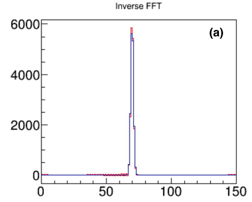
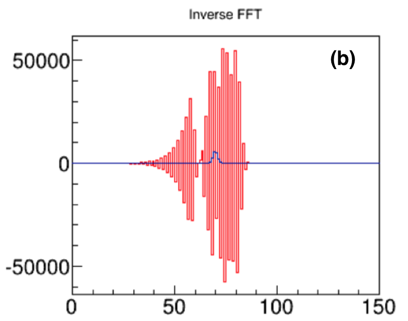
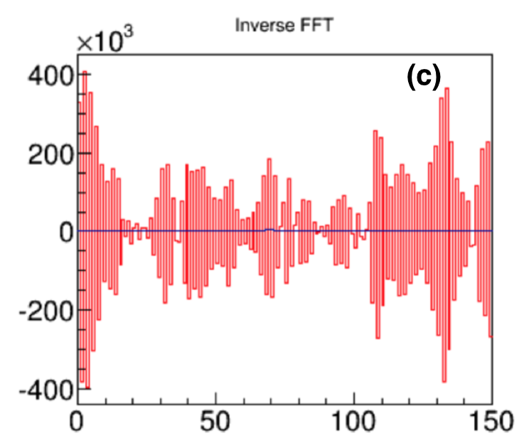
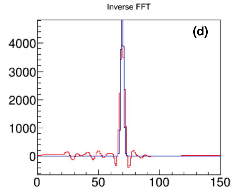
Figure 5: Effect of Signal Processing and Noise Filtering

The Wiener Filter function is optimized for different gain and shaping time settings for both induction and collection planes. The filter reduces the noise by a significant amount, however there is a loss in signal amplitude too. In order to preserve the signal strength and to obtain the true charge information from all the three planes, the filter is normalized in such a way so that it conserves the area. This step is very important in order to have a robust noise filter.

4 Additional Signal Processing Challenges

With the robust noise filtering and deconvolution, the full signal processing chain is complete and the desired charge signal is obtained from all three planes. There are still some additional challenges involved in the process. Due to the wire readout assembly of LArTPC, there is an effect of dynamic induced charge as ionized electrons traveling through the TPC wires induce signal not only on the closest wire but also on the adjacent wires. The field model described above does not take into account the charge contributions from the adjacent wires and treats signal from each TPC wire independently. To show the effect of induced current on the signal amplitude, Fig. 6 (left) shows the weighted equipotential contours (green) for a U-Plane wire superimposed on the electron drift lines (orange). The induced charge on each wire is derived using Eq. (6) along the drift line of each electron.

$$i=-q_{m}E_{w}.v_{d}$$ (6)

Fig. 6 (right) (b) shows the induced current waveform for a central U-Plane wire using the 2-D GARFIELD simulation for a track $1.7\degree$ from the vertical (shown in (a)). In comparison with the signal response in Fig. 3 (left), the induced charge signal is more complicated and strongly depends on the angle of the track.

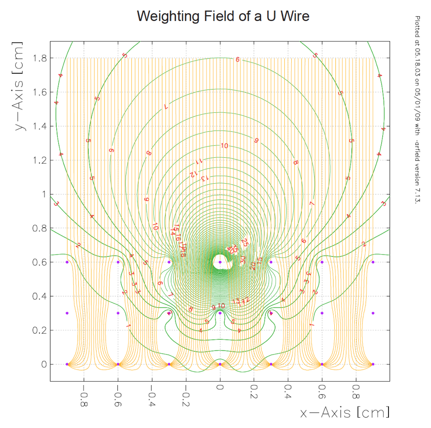
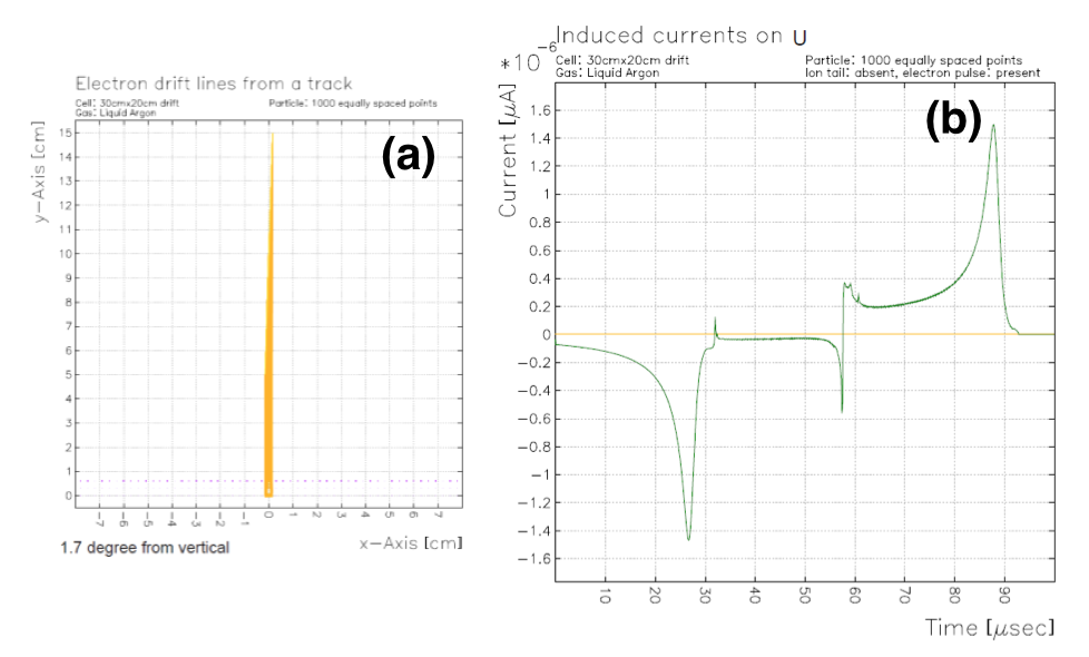
Figure 6: 2-D field simulations of the weighted potential distributions for a U-Plane wire. The weighed equipotential contours (green) are shown superimposed on the electron drift lines shown in orange (left); and (a) for a track $1.7\degree$ from the vertical, (b) the induced current waveform obtained from the Garfield simulation on the central U-Plane wire.

In order to account for the dynamic induced charge effect, the traditional deconvolution scheme described above is revised using the 2-D fast fourier transformation method in both time and wire parameter space. This implementation of a double deconvolution method is the most recent development in the LArSoft signal processing procedure.

5 New 3D Reconstruction with Charge and Time

After the robust signal processing chain, a new 3D event reconstruction method using both charge and time information is being developed. This new method is called “Wire-Cell Reconstruction” [13]. Reconstruction with a LArTPC wire plane readout is challenging due to inherent ambiguities/degeneracies when using a projective wire geometry. In particular, the timing information alone is not enough to remove various ambiguities in a complex electromagnetic shower consisting of many tracks. An example of such a degeneracy is illustrated in Fig. 7 (left) using only two wire planes for simplicity. The true hits are shown in red and the fake hits in blue. For a given time slice, a total of six possible hits on two U wires and three V wires generates ambiguation. This degeneracy increases exponentially with the increase in number of hits. Additional information is required in order to remove this degeneracy.

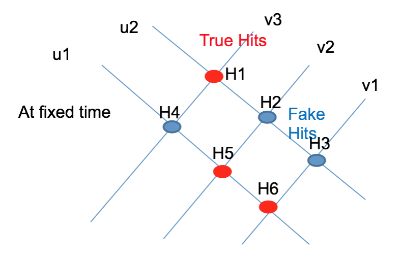
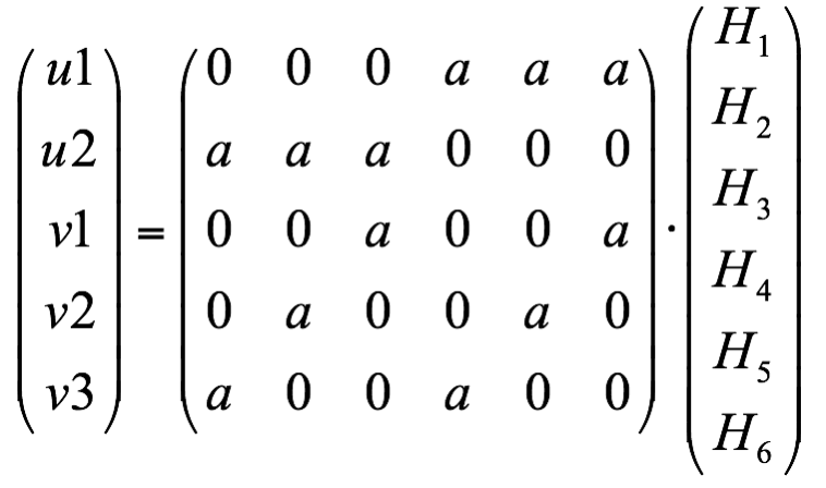
Figure 7: An example of hit degeneracy using two planes (left); and charge matrix equation to solve degeneracy (right)

Since the same charge is measured by all three wire planes, charge as well as time information can be reliably used to resolve this degeneracy. Fig. 7 (right) shows the charge matrix equations, where $u_{i}$, $v_{i}$ are the measured charges on the wires, $H_{i}$ matrix is the true charge to be resolved. After solving these 2D equations, the charge on the fake hits is expected to be close to zero and hence the degeneracy is greatly reduced. This technique is used to obtain 3D hit maps by combining results from different time slices. This new algorithm is under rapid development towards the goal of automated reconstruction for LArTPC.

6 Conclusions

The LArTPC is an excellent detector technology for precision neutrino physics measurements. The MicroBooNE experiment, being the first experiment in the future short baseline program at Fermilab is an important step in the development of LArTPC technologies for future multi-kiloton detectors, in addition to enabling a wide range of measurements of neutrino cross-sections and interactions. LArTPC signal processing is the first and a critical step in obtaining the correct charge and time information from all three wire planes. After robust signal processing, we have demonstrated that both the correct charge and time information on all 3 planes can be obtained and is available to be used in future improved 3-D tracking and calorimetry measurements.

References

- [1] C. Rubbia, “The Liquid Argon Time Projection Chamber: A New Concept for Neutrino Detectors,” CERN-EP-INT-77-08.
- [2] W. Willis and V. Radeka, Nuclear Instruments and Methods 120, no. 2, 221-236 (1974).
- [3] O. Bunemann, T.E. Cranshaw, J.A. Harvey, Can. J. Res. 27, 191 (1949).
- [4] H. Chen et al., “Proposal for a New Experiment Using the Booster and NuMI Neutrino Beamlines: MicroBooNE,” 2007. FERMILAB-PROPOSAL-0974.
-
[5]
MicroBooNE Technical Design Report,
http://www-microboone.fnal.gov/publications/TDRCD3.pdf - [6] V. Radeka et. al., “Cold Electronics for ’Giant’ Liquid Argon Time Projection Chambers,” J. Phys. Conf. Ser. 308 (2011) 012021.
- [7] J. Conrad et al., “The Photomultiplier Tube Calibration System of the MicroBooNE Experiment,” JINST 10, T06001 (2015).
- [8] R. Veenhof, “GARFIELD, recent developments,” Nucl. Instrum. Meth. A 419, 726 (1998).
- [9] E. D. Church, “LArSoft: A Software Package for Liquid Argon Time Projection Drift Chambers,” arXiv:1311.6774 [physics.ins-det].
- [10] B. Baller, “Liquid Argon TPC Signal Formation, Signal Processing and Reconstruction,” (under preparation).
- [11] Fast Fourier Transform, http://mathworld.wolfram.com/FastFourierTransform.html
- [12] Wiener, Norbert, “Extrapolation, Interpolation, and Smoothing of Stationary Time Series,” New York: Wiley. ISBN 0-262-73005-7 (1949).
- [13] Wire-Cell Reconstruction Package, http://www.phy.bnl.gov/wire-cell/