Kernel-Penalized Regression for Analysis of Microbiome Data

Abstract

The analysis of human microbiome data is often based on dimension-reduced graphical displays and clusterings derived from vectors of microbial abundances in each sample. Common to these ordination methods is the use of biologically motivated definitions of similarity. Principal coordinate analysis, in particular, is often performed using ecologically defined distances, allowing analyses to incorporate context-dependent, non-Euclidean structure. In this paper, we go beyond dimension-reduced ordination methods and describe a framework of high-dimensional regression models that extends these distance-based methods. In particular, we use kernel-based methods to show how to incorporate a variety of extrinsic information, such as phylogeny, into penalized regression models that estimate taxon-specific associations with a phenotype or clinical outcome. Further, we show how this regression framework can be used to address the compositional nature of multivariate predictors comprised of relative abundances; that is, vectors whose entries sum to a constant. We illustrate this approach with several simulations using data from two recent studies on gut and vaginal microbiomes. We conclude with an application to our own data, where we also incorporate a significance test for the estimated coefficients that represent associations between microbial abundance and a percent fat.

journalname

, , , and

1 Introduction

A common tool in the analysis of data from microbiome studies is a scatterplot of dimension-reduced microbial abundance vectors. This is a display of the samples’ beta diversity which, in ecology, refers to differences among various habitats. When applied to human studies, beta diversity describes the variation in microbial community structure across sampling units (e.g., human subjects): a beta diversity plot displays the $n$ sampling units with respect to the principal coordinates of their microbial abundance vectors, each consisting of measures on the $p$ taxa observed in the study; see, e.g., Claesson et al. (2012); Koren et al. (2013); Kuczynski et al. (2010); Goodrich et al. (2014). This principal coordinates analysis (PCoA; or multidimensional scaling, MDS) begins with an $n\times n$ matrix of pairwise dissimilarities between abundance vectors. The choice of dissimilarity measure may greatly influence the biological interpretation (Lozupone et al., 2007; Fukuyama et al., 2012). Euclidean distance is rarely used.

Dissimilarity measures that account for phylogenetic relationships among the taxa are assumed to enhance statistical analyses — for instance, to improve the power of statistical tests — because they incorporate the degree of divergence between sequences (Chen et al., 2012) and do not ignore “the correlation between evolutionary and ecological similarity” (Hamady and Knight, 2009). The UniFrac distance (Lozupone and Knight, 2005), in particular, is based on the premise that taxa which share a large fraction of the phylogenetic tree should be viewed as more similar than those sharing a small fraction of the tree. In the unweighted version of UniFrac, each taxon is quantified merely by its presence or absence; the distance between a pair of samples is based on the number of branches in the tree shared by both. Figure 1(a) is a beta diversity plot of $n=100$ human microbial abundance vectors with $p=149$ taxa based on data from Yatsunenko et al. (2012). The 2-dimensional coordinates of the samples are displayed with respect to the unweighted UniFrac distance, and each sample is colored according to the age of the subject.

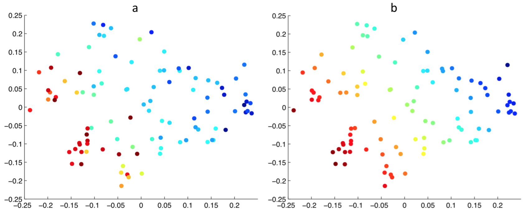
Figure 1: PCoA plots of data from Yatsunenko et al. (2012). (a): PCoA plot with respect to unweighted UniFrac distance, colored according to log(age) of subject. (b): PCoA plot with respect to unweighted UniFrac distance, colored according to $y_{\mbox{\footnotesize}True}$ from the model in Eq. (3.2) with $\epsilon=0$.

Dissimilarity measures in microbiome studies are many and varied, with a rich collection that, like UniFrac, exploit the phylogentic structure: Chen et al. (2012) generalize UniFrac by reweighting rare and abundant lineages; double principal coordinate analysis (DPCoA) (Pavoine, Dufour and Chessel, 2004), as shown by Purdom (2011), generalizes PCA by incorporating the covariance that would arise if the data was created by a process modeled by the tree; the edge PCA method of Matsen and Evans (2013) incorporates taxon abundance information at all nodes in a phylogenetic tree, rather than just the leaves of the tree, and Evans and Matsen (2012) formalize the mathematical interpretation of UniFrac as just one example within a large family of Wasserstein (or earth mover’s) metrics. A wide variety of non-phylogenetic dissimilarities are also in common use, such as Bray-Curtis (The Human Microbiome Project Consortium, 2012) and Jenson-Shannon (Koren et al., 2013), among others.

While PCoA plots provide valuable graphical insight into the relationships among microbial profiles and an outcome or phenotype, they do not quantify this association. More importantly, the (sets of) taxa associated with the outcome — and the magnitude or statistical significance of such associations — are not ascertained from a PCoA plot; once a matrix of (dis)similarities between samples is formed, it is not clear how to identify individual taxa that are associated with an outcome. Specifically, given a PCoA plot as in Figure 1(a), with structure imposed by the chosen dissimilarity matrix (e.g., unweighted UniFrac) and with associations implied by a class label or continuous outcome (e.g., age), how does one estimate which taxa or subcommunities are associated with this outcome? We address this question by formulating multivariate regression models that are constrained by the structure of the (dis)similarity matrix. This is made possible by exploiting an equivalence between a taxon-based (primal space) and sample-based (dual space) formulation of our penalized regression models. While exploiting such an equivalence is straightforward in the special case of ridge regression (with purely Euclidean structure), it becomes complicated when more general distance measures are used. To this end, we show how a little-used regularization scheme by Franklin (1978) provides a dual-space regression coefficient estimate that naturally connects to primal-space coefficients. Because a dissimilarity matrix can be used to construct a similarity matrix (as commonly done in classical MDS (Mardia, Kent and Bibby, 1980)), we work with kernels, rather than distances, and allow for general kernels, including those constructed from a nonlinear feature map.

In addition to complications stemming from more general distances, the analysis of microbiome data is also complicated by the compositional nature of the data itself. More specifically, taxon measures typically represent relative, rather than absolute, abundances. The $p$-variate relative abundance vectors are thus compositional in that they are constrained to a simplex within $\mathbb{R}^{p}$; such data do not reside in a Euclidean vector space (Aitchison, 2003a). Consequently, spurious correlations arise and standard multiple regression models fail. Our proposed KPR framework, however, addresses this: the centered log (CLR) transform of the relative abundance vectors first removes the vectors from the simplex, then the estimation process is constrained using a penalization term defined by Aitchison’s variation matrix. This approach takes a different perspective from the recent proposal of Li (2015) which forces the estimated coefficient vector to reside in the simplex. Given that the CLR transforms the compositional vectors to Euclidean space and that the units of the Aitchison variation matrix are the same as the CLR transformed data (Egozcue and Pawlowsky-Glahn, 2011), our constraint seems more suitable for the geometry of the problem.

In summary, we describe a family of high-dimensional regression problems in Section 2, which are designed to incorporate the assumptions that are tacitly implied by various exploratory and graphically-focused PCoA plots common in microbiome studies. We show how phylogenetic and other structure can be incorporated via kernel penalized regression in either the primal ($p$-dimensional) feature space or the dual ($n$-dimensional) samples space; see Sections 2.2 and 2.3. Finally, our proposed framework leads to an approach, described in Section 2.4, for addressing well-known problems that arise from applying standard (Euclidean-based) statistical models to compositional data. Section 3 illustrates the proposed framework with simulations based on publicly available data, while Section 4 presents an application to our recent microbiome study of premenopausal women. In this analysis, we obtain estimates of associations between microbial species and percent fat measured in premenopausal women, and also provide inference for these estimates by applying a recent significance test (Zhao and Shojaie, 2016) in our kernel-penalized regression (KPR) framework.

2 Kernel Penalized Regression for Microbiome Data

We describe a family of multiple regression problems aimed at incorporating assumptions that are implicit in PCoA plots common in microbiome studies. We begin in Section 2.1 by establishing notation and concepts from existing dimension-reduction (ordination) methods with the goal of extending them to non-truncated (penalized) regression models. Section 2.2 extends PCoA and PCR to penalized regression models in the primal space in a manner that incorporate structures implicit in recent microbiome analyses. Section 2.3 extends kernel ridge regression to general (non-$L^{2}$) structure and the use of two kernels. This extension exploits a dual-space regularization scheme of Franklin (Franklin, 1978). Section 2.4 describes how our proposed framework can be applied to formulate a penalized regression model that accounts for the structure of compositional data.

We denote by $y_{i}$, $i=1,..,n$, a real-valued quantified trait, and by $x_{i}=[x_{i1},...,x_{ip}]^{\prime}$ a $p$-dimensional vector of microbial abundance values measured for each of $n$ subjects. Denote by $X$ the $n\times p$ sample-by-taxon matrix whose $i$th row is $x_{i}^{\prime}$. We assume throughout that the columns of $X$ are mean centered. For now, we assume that the abundance values are appropriately normalized/transformed and postpone the treatment of compositional data to Section 2.4. The transpose of a matrix $A$ is denoted by $A^{\prime}$ and the Frobenius norm is denoted as $\|A\|_{F}$. The Euclidean norm of a vector $x\in\mathbb{R}^{p}$ is denoted $\|x\|_{\mathbb{R}^{p}}$, $\|x\|_{2}$ or simply $\|x\|$.

2.1 Background for PCoA and principal component regression

Consider first the Euclidean PCoA, which is obtained from the eigenvectors of the kernel matrix $K_{I}:=XX^{\prime}$ of inner products $K_{ij}=\langle x_{i},x_{j}\rangle$ between samples. Let $\mathcal{J}$ be the centering matrix, $\mathcal{J}=I-\frac{1}{n}\boldsymbol{1}\boldsymbol{1}^{\prime}$, where $\boldsymbol{1}$ is the $n\times 1$ vector of ones. Then, it can be seen that $XX^{\prime}=-\frac{1}{2}\mathcal{J}\Delta^{E}\mathcal{J}$, where $\Delta^{E}$ is the $n\times n$ matrix of squared Euclidean distances between samples: $\Delta^{E}_{i,j}=\|x_{i}-x_{j}\|_{\mathbb{R}^{p}}^{2}$. The relationship between a kernel and a distance matrix $\Delta$ is more general. In particular, if $\Delta$ is any $n\times n$ symmetric matrix of squared dissimilarities between vectors in $\mathbb{R}^{p}$ then $H=-\frac{1}{2}\mathcal{J}\Delta\mathcal{J}$ serves as a kernel matrix summarizing similarities; see, e.g., Gower (1966); Pekalska, Paclik and Duin (2002). A particular case involves a $p\times p$ symmetric, positive definite matrix $Q$ that defines an inner product $\langle x_{i},x_{j}\rangle_{Q}=x_{i}^{\prime}Qx_{j}$ on $\mathbb{R}^{p}$. If $\Delta^{Q}$ denotes the matrix of squared distances, $\Delta^{Q}_{i,j}=\|x_{i}-x_{j}\|_{Q}^{2}=\langle x_{i}-x_{j},x_{i}-x_{j}\rangle_{Q}$, defined with respect to this inner product, then $XQX^{\prime}=-\frac{1}{2}\mathcal{J}\Delta^{Q}\mathcal{J}$ is also a similarity kernel for the $n$ samples. We will denote this kernel by $K_{Q}=XQX^{\prime}$. Similarly, one may start with a matrix $\Delta^{U}$ of squared distances defined by a tree-based UniFrac dissimilarity (Lozupone and Knight, 2005), and define a similarity kernel by $H=-\frac{1}{2}\mathcal{J}\Delta^{U}\mathcal{J}$.

In graphical displays, two or three coordinates are typically used to explore the relationship between samples. Let $K=US^{2}U^{\prime}$ be the eigen-decomposition of any similarity kernel, $K$, where $U$ is the matrix whose columns are eigenvectors and $S^{2}=\mathop{\rm diag}\{\sigma_{j}^{2}\}$ is the diagonal matrix of eigenvalues. The two-dimensional PCoA plot is then the collection of points $\{\eta_{i1},\eta_{i2}\}_{i=1}^{n}:=\{(\sigma_{1}U_{i1},\sigma_{2}U_{i2})\}_{i=1}^{n}$; i.e., a plot of the points represented by the first two columns of the matrix $US$. These points are often colored according to a grouping label or continuous value, $\{y_{i}\}_{i=1}^{n}$, to graphically explore the existence of an association between the outcome $y$ and the sample profiles summarized by the first few columns of $US$. So, a PCoA plot is a graphical depiction of a two-component regression model of association:

$$y_{i}=\gamma_{1}\eta_{i1}+\gamma_{2}\eta_{i2}+\epsilon,\quad i=1,\ldots,n,$$ (2.1)

where $\eta_{1}$ and $\eta_{2}$ are the first two PCoA axes. Ordinary principal component regression (PCR) corresponds to the case that $\eta_{1}$ and $\eta_{2}$ come from the Euclidean kernel $K_{I}=XX^{\prime}$. On the other hand, the configuration of points in Figure 1(b) correspond to the first two eigenvectors of the kernel defined by an unweighted UniFrac distance matrix $\Delta^{U}$, and colors of individual points correspond to the values of $y$ from eq. (2.1) with $\epsilon=0$.

Let $A_{(k)}$ denote the first $k$ columns of a matrix $A$, or its first $k$ rows and columns if $A$ is diagonal. Then, using the singular value decomposition (SVD), $X=USV^{\prime}$, if we express the dimension-reduced approximation of $X$ as $\breve{X}:=U_{(2)}S_{(2)}V_{(2)}^{\prime}$, then eq. (2.1) can be written as

$$y =\gamma_{1}\eta_{1}+\gamma_{2}\eta_{2}+\epsilon$$ (2.2)

$$=U_{(2)}S_{(2)}\,\gamma+\epsilon$$

$$=\breve{X}V_{(2)}\,\gamma+\epsilon,$$

where $\gamma=[\gamma_{1}\ \gamma_{2}]^{\prime}$. Here, $\breve{X}V_{(2)}=U_{(2)}S_{(2)}$, and $\mathop{\rm Range}(\breve{X}^{\prime})=\mathop{\rm Range}(V_{(2)})$. Therefore, assuming a coefficient vector $\beta$ of the form $\beta=\breve{X^{\prime}}\gamma$, the model $y=\breve{X}V_{(2)}\,\gamma+\epsilon$ can be written as $y=\breve{X}\beta+\epsilon$. So inherent in a Euclidean PCoA plot is an implicit coefficient vector, $\beta$, which models a linear association between $y$ and $\breve{X}$. Using the SVD of $X$ in (2.2), the PCR estimate of $\beta\in\mathbb{R}^{p}$ is expressed as

$$\hat{\beta}_{\mbox{\tiny PCR}}=(\breve{X}^{\prime}\breve{X})^{{\dagger}}\breve{X}^{\prime}y=V_{(2)}S_{(2)}^{-1}U_{(2)}^{\prime}y=\sum_{k=1}^{2}\frac{1}{\sigma_{k}}u_{k}^{\prime}y\,v_{k},$$ (2.3)

where ${\dagger}$ denotes the Moore-Penrose inverse.

2.2 Penalized regression and DPCoA

An alternative to a Euclidean PCR is the ordinary ridge regression (Hoerl and Kennard, 1970),

$$\hat{\beta}_{\mbox{\tiny ridge}}=(X^{\prime}X+\lambda I)^{-1}X^{\prime}y=\sum_{k=1}^{n}\left(\frac{\sigma_{k}^{2}}{\sigma_{k}^{2}+\lambda^{2}}\right)\frac{1}{\sigma_{k}}u_{k}^{\prime}y\,v_{k},$$ (2.4)

in which the terms are re-weighted instead of being truncated, as in $\hat{\beta}_{\mbox{\tiny PCR}}$. The estimate in (2.4) is the solution of the penalized least squares regression problem, $\hat{\beta}_{\mbox{\tiny ridge}}=\mathop{\rm arg\,min}_{\beta}\left\{\|y-X\beta\|^{2}+\lambda\|\beta\|^{2}\right\}$, where here and throughtout $\lambda$ is a tuning parameter that controls the amount of shrinkage or size of $\beta$ in the penalty term. Here the penalty is simply the Euclidean (or $\ell^{2}$) norm on $\mathbb{R}^{p}$, but a wide range of penalty terms have been proposed to replace or extend this particular form of regularization; see Bühlmann, Kalisch and Meier (2014) for a review of the most established methods. These methods, such as the lasso, elastic net or SCAD do not incorporate any extrinsic information, but a variety of other penalization methods have been proposed which aim to do this. For instance, Tanaseichuk, Borneman and Jiang (2014) uses a tree-guided penalty (Kim and Xing, 2010) to incorporate such structure into a penalized logistic regression framework to encourage similar coefficients among taxa according to their relationships in the phylogenetic tree. Tibshirani and Taylor (2011) study the solution path for computing a “generalized lasso” estimate in which an $\ell^{2}$ penalty is replaced with an $\ell^{1}$ penalty applied to a linear transformation of the features, $\lambda\|L\beta\|_{1}$. Within the context of genetic networks, Li and Li (2008) accounted for network structure by augmenting the $\ell^{1}$ penalty with a second penalty of the form $\lambda_{2}\|\beta\|_{\mathcal{L}}^{2}=\beta^{\prime}\mathcal{L}\beta$, where $\mathcal{L}$ denotes the graph Laplacian matrix corresponding to pre-defined connections between genes in a pathway.

For now, we consider a positive definite $p\times p$ matrix $Q$ with a Cholesky decomposition $Q=LL^{\prime}$, and a penalty term of the form $\|L^{-1}\beta\|^{2}=\|\beta\|^{2}_{Q^{-1}}=\beta^{\prime}Q^{-1}\beta$. The generalized ridge (or Tikhonov regularization (Golub and van Loan, 2012)) estimate with respect to $Q$ is then defined as

$$\hat{\beta}_{Q} =\mathop{\rm arg\,min}_{\beta}\{\|y-X\beta\|^{2}+\lambda\|\beta\|_{Q^{-1}}^{2}\}=(X^{\prime}X+\lambda Q^{-1})^{-1}X^{\prime}y$$ (2.5)

$$=\sum_{k=1}^{n}\left(\frac{\sigma_{k}^{2}}{\sigma_{k}^{2}+\lambda\mu_{k}^{2}}\right)\frac{1}{\sigma_{k}}u_{k}^{\prime}y\,v_{k},$$

This estimate takes the same form as (2.4) but now the vectors $u_{k}$ and $v_{k}$ arise from the SVD of $XL=USV^{\prime}$.

As an aside, it is worth noting that if $A$ denotes any matrix with $p$ columns, the structure of an estimate $\hat{\beta}_{A}$ from a penalty term of the form $\|A\beta\|_{2}^{2}$ is determined by the joint eigenstructure of the pair $(X,A)$ via the generalized singular value decomposition. In particular, the basis expansion of $\hat{\beta}_{Q}$ in (2.5) is given in terms of the generalized singular vectors of $(X,L^{-1})$. Although the ridge estimate (with $Q=I_{p}$) is biased, an informed choice of penalty term can, in fact, reduce the bias (Randolph, Harezlak and Feng, 2012).

Now consider the context of phylogentic information and let $\delta$ represent the matrix of squared patristic distances between pairs of taxa — i.e., the sum of branch lengths between each pair of taxa on the leaves of a phylogenetic tree. Set $Q=-\frac{1}{2}\mathcal{J}\delta\mathcal{J}$, a matrix of similarities between taxa. Double principal coordinate (DPCoA) analysis was proposed as a multi-step procedure by Pavoine, Dufour and Chessel (2004) to provide an alternative to ordinary PCoA by incorporating both the structure among samples and the structure implied by species distribution among subcommunities; i.e., the phylogeny as summarized by $Q$. Purdom (2011) clarified the original multi-step DPCoA procedure and showed how it can be more simply understood as a generalized PCA (gPCA) in which one obtains the new coordinates from the eigenvectors of $K_{Q}=XQX^{\prime}$. Note that when $Q$ is the identity matrix ($Q=I_{p}$), DPCoA reduces to PCA/MDS. As emphasized in Purdom (2011), the use of a non-identity $Q$ matrix incorporates structure from known relationships between the $p$ taxa by exploiting a matrix representation of phylogenetic relationships, thus providing a model for covariance structure.

If we let $Q=LL^{\prime}$ be a Cholesky decomposition of $Q$ and set $Z:=XL$, then the kernel $K_{Q}$ has an SVD of the form $XQX^{\prime}=VS^{2}V^{\prime}$. This leads to a two-dimensional regression estimate that takes the same the form as $\hat{\beta}_{\mbox{\tiny PCR}}$ in (2.3). Indeed, we can recover a primal space estimate in terms of singular vectors as

$$\hat{\beta}_{\mbox{\tiny DPCR}}:=V_{(2)}S_{(2)}^{-1}U_{(2)}^{\prime}y=\sum_{k=1}^{2}\frac{1}{\sigma_{k}}u_{k}^{\prime}y\,v_{k}.$$ (2.6)

That is, implicit in a DPCoA plot is a coefficient vector, $\hat{\beta}_{\mbox{\tiny DPCR}}$ which models a two-dimensional linear association between $y$ and $Z=XL$ in the same way that $\hat{\beta}_{\mbox{\tiny PCR}}$ represents a two-dimensional linear association between $y$ and $X$. Further, $XQX^{\prime}=(XL)(XL)^{\prime}$ and so $U$, $S$ and $V$ in (2.6) are the same as those in the penalized (non-truncated) estimate, $\hat{\beta}_{Q}$, in (2.5).

2.3 Kernel-based regression with two kernels

In addition to similarities among taxa, as in $Q$, it is often of interest to incorporate similarities among samples as derived, for instance, from UniFrac distances: $H=-\frac{1}{2}\mathcal{J}\Delta^{U}\mathcal{J}$. The symmetric positive definite $n\times n$ kernel $H$ defines a new inner product on $\mathbb{R}^{n}$ given by $\langle u,w\rangle_{H}=u^{\prime}Hw$, with the corresponding norm $\|u\|^{2}_{H}=\langle u,u\rangle_{H}$. If we consider both a general kernel, $H$, and a DPCoA kernel $K_{Q}=XQX^{\prime}$, the generalized ridge estimate $\hat{\beta}_{Q}$ in (2.5) can be extended to

$$\hat{\beta}_{Q,H} :=\mathop{\rm arg\,min}_{\beta\in\mathbb{R}^{p}}\left\{\|y-X\beta\|_{H}^{2}+\lambda\|\beta\|_{Q^{-1}}^{2}\right\}$$ (2.7)

$$=(X^{\prime}HX+\lambda Q^{-1})^{-1}X^{\prime}Hy.$$

In this section, we show that the estimate in (2.7) is directly defined based on the generalized eigenvectors of the two kernels $Q$ and $H$. Before proceeding to the general case, let us examine the special case of ridge regression. In this case, $H=I_{n}$ and $Q=I_{p}$. It is well known that ridge estimates can be obtained by solving an equivalent optimization problem in the dual space $\mathbb{R}^{n}$, known as kernel ridge regression (Schölkopf and Smola, 2002). Specifically, taking $K_{I}=XX^{\prime}$, the ridge estimate in (2.4) can be obtained as $\hat{\beta}_{\mbox{\tiny ridge}}=X^{\prime}\hat{\gamma}_{\mbox{\tiny kernel ridge}}$, where

$$\hat{\gamma}_{\mbox{\tiny kernel ridge}} =(K_{I}+\lambda I)^{-1}y=(K_{I}^{2}+\lambda K_{I})^{-1}K_{I}y$$ (2.8)

$$=\mathop{\rm arg\,min}_{\gamma\in\mathbb{R}^{n}}\{\|y-K_{I}\gamma\|^{2}+\lambda\|\gamma\|^{2}_{K_{I}}\}.$$

In the case of ridge, the connection between the dual- and primal-space estimates, $\hat{\gamma}_{\mbox{\tiny kernel ridge}}$ and $\hat{\beta}_{\mbox{\tiny ridge}}$, relies on the form $K_{I}=XX^{\prime}$. Unfortunately, it is less clear how to extend this connection to a general kernel (e.g., UniFrac or polynomial). One way to incorporate a general kernel $K$ and a second kernel $H$ in (2.8) is to define the penalty in terms of $H$ as

$$\hat{\gamma}_{*}=(K^{2}+\lambda H^{-1})^{-1}Ky=\mathop{\rm arg\,min}_{\gamma}\{\|y-K\gamma\|^{2}+\lambda\|\gamma\|_{H^{-1}}^{2}\},$$ (2.9)

which is exactly the Tikhonov regularization, but in the dual space; compare eq. (2.5). However, $\hat{\gamma}_{*}\in\mathbb{R}^{n}$ has no obvious connection to a penalized estimate of $\beta\in\mathbb{R}^{p}$ and cannot be used to obtain a penalized regression estimate in the primal space, even if $K=K_{I}=XX^{\prime}$.

To bridge this gap, we instead apply the Franklin regularization scheme (Franklin, 1978), a little-used alternative to Tikhonov regularization. More specifically, for any kernels $K$ and $H$, we define the dual estimate

$$\hat{\gamma}_{H,K}:=(K+\lambda H^{-1})^{-1}y=\mathop{\rm arg\,min}_{\gamma\in\mathbb{R}^{n}}\{\|y-K\gamma\|_{K^{-1}}^{2}+\lambda\|\gamma\|_{H^{-1}}^{2}\}$$ (2.10)

Comparing (2.9) and (2.10), one sees that the analytic form of (2.10) involves just $K$ rather than $K^{2}=K^{\prime}K$. As shown in Proposition 2.2, this subtle difference is a key for relating $\hat{\gamma}_{H,K}$ and its primal-space counterpart. Before presenting the main result of this section, we provide several equivalent forms of $\hat{\gamma}_{H,K}$.

$$\hat{\gamma}_{H,K} =(K+\lambda H^{-1})^{-1}y$$ (2.11)

$$=\mathop{\rm arg\,min}_{\gamma\in\mathbb{R}^{n}}\{\|y-K\gamma\|_{K^{-1}}^{2}+\lambda\|\gamma\|_{H^{-1}}^{2}\}$$

$$=\mathop{\rm arg\,min}_{\gamma\in\mathbb{R}^{n}}\{\|y-K\gamma\|_{H}^{2}+\lambda\|\gamma\|_{K}^{2}\}$$

$$=(HK+\lambda I)^{-1}Hy$$

$$=H(KH+\lambda I)^{-1}y.$$

In Proposition 2.2, we also refer to the special case corresponding to the DPCoA ordination. As before, let $Z=XL$ so that $K_{Q}=XQX^{\prime}=XLL^{\prime}X^{\prime}=ZZ^{\prime}$. Taking $H=I$, the dual-space estimate in (2.10) is $\hat{\gamma}_{I,K_{Q}}=(K_{Q}+\lambda I)^{-1}y$, and so the corresponding primal-space estimate is $\hat{\beta}\equiv Z^{\prime}\hat{\gamma}_{I,K_{Q}}$. Since this estimate arises from the DPCoA kernel, so we make the following definition.

Definition 2.1.

A primal space DPCoA estimate is of the form $\hat{\beta}_{\mbox{\tiny DPCoA}}=Z^{\prime}\hat{\gamma}_{I,K_{Q}}=L^{\prime}X^{\prime}(XQX^{\prime}+\lambda I)^{-1}y$.

The next proposition collects several properties that emphasize the roles of $H$ and $K$ in our penalized regression framework. In particular, we show that the primal space estimate $\hat{\beta}_{Q,H}$ can be recovered in terms of two kernels, $H$ and $K_{Q}$.

Proposition 2.2.

Let $H$ and $K$ be any two kernels constructed using the rows of $X$ in the regression model $y=X\beta+\epsilon$. Then,

1. $\hat{\gamma}_{H,K}$ is a linear combination of the eigenvectors of the matrix product $HK$.

2. For any kernel $H$ and DPCoA kernel $K_{Q}=XQX^{\prime}$, then the primal- and dual-space estimates in (2.7) and (2.10), respectively, are related as: $\hat{\beta}_{Q,H}=QX^{\prime}\hat{\gamma}_{H,K_{Q}}$.

3. For $H=I$ and $Q=LL^{\prime}$, the generalized ridge and DPCoA estimates are related as $\hat{\beta}_{Q}=QX^{\prime}(K_{Q}+\lambda I_{n})^{-1}y=L\hat{\beta}_{\mbox{\tiny DPCoA}}$.

Proof.

These relationships are based on several basic linear algebraic properties. In particular, we make use of the following identities:

$$(X^{\prime}HX+\lambda Q^{-1})^{-1}X^{\prime}H=(QX^{\prime}HX+\lambda I_{p})^{-1}QX^{\prime}H$$ (2.12)

$$=Q(X^{\prime}HXQ+\lambda I_{p})^{-1}X^{\prime}H=QX^{\prime}(XQX^{\prime}+\lambda H^{-1})^{-1}$$

$$=QX^{\prime}H(XQX^{\prime}H+\lambda I_{n})^{-1}.$$

1. Let $w_{1},...,w_{n}$ denote the columns of the matrix $W$ satisfying $W^{\prime}KW=\mathop{\rm diag}\{\sigma_{1},...,\sigma_{n}\}$ and $W^{\prime}H^{-1}W=\mathop{\rm diag}\{\mu_{1},...,\mu_{n}\}$. That is, $\{w_{k}\}$ is a basis with respect to which a simultaneous diagonalization of $K$ and $H^{-1}$ is obtained (see Golub and van Loan (2012); Hansen (1998)). These are the generalized eigenvectors of the pair $(K,H^{-1})$. Then

   $$\hat{\gamma}_{H,K}=\sum_{k=1}^{n}\left(\frac{\sigma_{k}}{\sigma_{k}+\lambda\mu_{k}}\right)\frac{w_{k}^{\prime}y}{\sigma_{k}}w_{k}.$$ (2.13)

   Since $H$ is invertible, the $w_{k}$’s are also eigenvectors of $HK$ (Golub and van Loan, 2012).

2. Using the identities in (2.12), the estimate in (2.7) can be expressed as

   $$\hat{\beta}_{Q,H} =Q(X^{\prime}HXQ+\lambda I_{p})^{-1}X^{\prime}Hy$$ (2.14)

   $$=QX^{\prime}(XQX^{\prime}+\lambda H^{-1})^{-1}y$$

   $$=QX^{\prime}(K_{Q}+\lambda H^{-1})^{-1}y=QX^{\prime}\hat{\gamma}_{H,K_{Q}}.$$

3. Setting $H=I$ in the first line of the above equalities gives $\hat{\beta}_{Q}=QX^{\prime}(XQX^{\prime}+\lambda I_{n})^{-1}y$. Using $Q=LL^{\prime}$ gives $\hat{\beta}_{Q}=L\,L^{\prime}X^{\prime}(K_{Q}+\lambda I_{n})^{-1}y=L\,Z^{\prime}(ZZ^{\prime}+\lambda I)^{-1}y=L\hat{\beta}_{\mbox{\tiny DPCoA}}$.

∎

Remarks:

1. Types of similarity kernels. In general, a sufficient condition for a matrix $K$ to be a similarity kernel is that it is induced by a feature map $\phi\colon\mathbb{R}^{p}\to\mathcal{K}$. More specifically, the $i,j$ entry of $K$ is defined as the inner product of the observations $x_{i}\in\mathbb{R}^{p}$ with respect to their transformed versions $K_{ij}=\langle\phi(x_{i}),\phi(x_{j})\rangle$ in the new inner product space, $(\mathcal{K},\langle\cdot,\cdot\rangle)$. Examples include $K_{I}=XX^{\prime}$ or $K_{Q}=XQX^{\prime}$, where $\mathcal{K}$ is $\mathbb{R}^{p}$ with inner product $\langle\cdot,\cdot\rangle_{Q}$ (as in DPCoA). It is this quadratic form that we require for $K_{Q}$ in Proposition 2.2(2)–(3); see Freytag et al. (2014) for genomic applications of this form. On the other hand, $H$ can be any symmetric positive semi-definite matrix. Here, we are more interested in biologically-motivated kernels, such as UniFrac or DPCoA, than mathematically-derived ones, such as those constructed from polynomials or radial basis functions (Schölkopf and Smola, 2002).

2. Co-informative kernels and the HSIC. Any kernels $K$ and $H$ may be used in (2.10) and (2.11), but to be useful in this framework, we assume that they are “co-informative” in the sense that they exhibit a shared eigenstructure; for instance, both should be informative for classifying samples. This concept is illustrated in the simulation of Section 3.3 and Figure 4. The co-informativeness can be made precise using the Hilbert-Schmidt information criteria (HSIC) (Gretton et al., 2005) or its relatives the distance covariance (Székely and Rizzo, 2009) or RV statistic (Robert and Escoufier, 1976). Josse and Holmes (2014) provide a nice review of these and related kernel-based tests. The HSIC provides a test for the statistical dependence of two data sets, $X_{1}$ ($n\times p$) and $X_{2}$ ($n\times q$), and is based on the eigen-spectrum of covariance operators defined by kernels defined by $X_{1}$ and $X_{2}$, respectively. For two kernels $K$ and $H$, the empirical HSIC is simply $\mathop{\rm trace}(HK)$. The HSIC is thus of particular interest in item (1) of Proposition 2.2, which shows how two co-informative kernels may be used to obtain a penalized estimate $\hat{\beta}_{Q,H}$.

3. Linear mixed models and KPR. As an alternative to the regularization framework presented here, it may be useful to consider a kernel as a generalized covariance among either the $p$ variables (using $Q$) or $n$ subjects (using $H$) (Purdom, 2011; Schaid, 2010). This alternative representation can be made precise using the linear mixed model (LMM) framework (Ruppert, Wand and Carroll, 2003). Specifically, recall from equations (2.7) and (2.11) that

   $$\hat{\beta}_{Q,H} =\mathop{\rm arg\,min}_{\beta\in\mathbb{R}^{p}}\{\|y-X\beta\|_{H}^{2}+\lambda\|\beta\|_{Q^{-1}}^{2}\}$$

   $$=QX^{\prime}(K_{Q}+\lambda H^{-1})^{-1}y$$

   $$=QX^{\prime}\mathop{\rm arg\,min}_{\gamma\in\mathbb{R}^{n}}\{\|y-K_{Q}\gamma\|_{H}^{2}+\lambda\|\gamma\|_{K_{Q}}^{2}\}=QX^{\prime}\hat{\gamma}_{H,K_{Q}}.$$

   These regression estimates are compatible with $\beta\sim N(0,\sigma_{b}^{2}Q)$,  $\epsilon\sim N(0,\sigma_{e}^{2}H^{-1})$ and $var(y)=(\tau K_{Q}+\lambda H^{-1})^{-1}$. And the estimate $\hat{\gamma}_{H,K_{Q}}$ is compatible with $\gamma\sim N(0,\sigma_{a}^{2}K_{Q}^{-1})$ and $\epsilon\sim N(0,\sigma_{e}^{2}H^{-1})$. With regard to the latter, a genetic similarity between subjects (e.g., kinship) is often used for grouping subjects and several authors have proposed this form of kernel for testing the (global) genetic association with a trait or phenotype, $y$; see, e.g., Schifano et al. (2012). In particular, these methods use the LMM framework to motivate and define a “kernel association test”. The variance score statistic for testing the null hypothesis of no association between $y$ and $X$ ($H_{0}:\beta=0$) is, using our notation above, $\mathcal{T}:=\|y\|_{H^{1/2}K_{Q}H^{1/2}}^{2}$. The kernel association testing framework has been applied to microbiome data using a single kernel at a time derived from Unifrac (Zhao et al., 2015), but this is a test for whether $\beta\neq 0$ and, unlike our KPR framework, provides no insight about which taxa, as represented by coordinates of $\beta$, are associated with $y$.

2.4 Regression with compositional data

Data from 16S rRNA gene sequencing methods are random counts of the molecules in each sample. The number of sequence reads assigned to a taxon contains no information about the actual number of molecules in the sample; the total number of reads observed in two samples can vary by several orders of magnitude. Hence, only relative amounts can be investigated. Common approaches for normalizing these data include converting them to proportions (relative percent) or subsampling the sequences to create equal library sizes for each sample (rarefying). These data are “compositional” in the sense that the microbial abundances represent a proportion of a constant total. It is well known, however, that compositional measures can result in spurious correlations among taxa (Pearson, 1896; Aitchison, 2003a; Friedman and Alm, 2012), an effect that can be quite extreme when there are a few dominant taxa.

Compositional data reside on the simplex $\mathbb{S}^{p-1}$ of unit-sum vectors in $\mathbb{R}^{p}$ and so standard multivariate methods do not apply (Aitchison, 2003b; Egozcue and Pawlowsky-Glahn, 2011; Li, 2015; Lovell et al., 2015). In particular, because these data do not naturally reside in a Euclidean vector space, standard regression models based on Euclidean covariance measures are inappropriate. However, ordinary least-squares and ridge regression estimates are of the form $\hat{\beta}=(X^{\prime}X+\lambda I)^{-1}X^{\prime}y$ (with $\lambda=0$ and $\lambda>0$, respectively). Thus, these estimates depend on the empirical covariance structure, $X^{\prime}X$, among taxa, which may include spurious correlations. Similarly, Li (2015) points out that a naïve application of lasso regression is not expected to perform well due to the compositional nature of the covariates. He addresses this issue by applying a lasso regression model to the log-ratio abundances and imposing an additional constant-sum constraint on the coefficient vector, $\beta$.

We next show that the generality of KPR for handling non-Euclidean structures can be used to address the compositional nature of microbiome data. In particular, we propose an approach that uses the centered log-ratio transformation of the compositional vectors and an estimate of covariance among the log taxa counts that is obtained via Aitchison’s variance matrix (Aitchison, 2003b; Egozcue and Pawlowsky-Glahn, 2011).

Let $X$ be the $n\times p$ sample-by-taxon matrix whose rows are relative percent (compositional) vectors $\{x_{i}\}_{i=1}^{n}\subset\mathbb{S}^{p-1}$. The columns of $X$ will be denoted by $x^{k}$, corresponding to $k=1,...,p$ taxa. Let $g(z)=\left(\Pi_{k=1}^{p}z^{k}\right)^{1/p}$ be the geometric mean of a row vector, $z$, and denote the centered log-ratio (CLR) transform of $x_{i}$ by $\tilde{x}_{i}=\mathop{\rm clr}(x_{i}):=\left[\log\frac{x_{i}^{1}}{g(x_{i})},\ldots,\log\frac{x_{i}^{p}}{g(x_{i})}\right]$. In what follows we denote the matrix of CLR vectors by $\tilde{X}$, and use the normalized variation matrix $T$, of $X$, as defined by Aitchison (1982): $T_{k,\ell}=\mathop{\rm var}\left(\frac{1}{\sqrt{2}}\log\frac{x^{k}}{x^{\ell}}\right)$. $T$ is a symmetric dissimilarity matrix with zeros on the diagonal and entries that have squared Aitchison distance units: the Aitchison norm of a vector $x\in\mathbb{S}^{p-1}$ is defined as $\|x\|_{a}^{2}=\frac{1}{2p}\sum_{k,\ell}\left(\log\frac{x^{k}}{x^{\ell}}\right)^{2}$. In fact, $\|x\|_{a}^{2}=\|\mathop{\rm clr}(x)\|^{2}$. One can show that $T$ is related to the covariance matrix, $C$ of the log of the true unobserved taxa counts via $T=v\boldsymbol{1}^{\prime}+\boldsymbol{1}v^{\prime}-2C$ (Li, 2015). Consequently, $C=-\frac{1}{2}\mathcal{J}T\mathcal{J}$, and we can use $C$ in place of $Q$ in eq. (2.5) to obtain

$$\tilde{\beta}_{C}=\mathop{\rm arg\,min}_{\beta}\left\{\|y-\tilde{X}\beta\|_{\mathbb{R}^{n}}^{2}+\lambda\|\beta\|_{C^{-1}}^{2}\right\}.$$ (2.15)

As a comparison, we observe that Li (2015) proposed a constrained regression

$$\mathop{\rm E}(y_{i})=\beta_{1}\log x_{i}^{1}+\dots+\beta_{p}\log x_{i}^{p}\quad\text{ subject to }\sum_{j=1}^{p}\beta_{j}=0,$$ (2.16)

augmented with a lasso penalty to obtain an estimate of the form

$$\mathop{\rm arg\,min}_{\beta}\left\{\frac{1}{2n}\|y-\sum_{j}\log(x^{j})\beta_{j}\|_{\mathbb{R}^{n}}^{2}+\lambda\sum_{j}|\beta_{j}|\right\}\quad\mbox{ subject to }\sum_{j=1}^{p}\beta_{j}=0.$$

The zero-sum constraint on $\beta$ was emphasized for interpretability advantages over the standard lasso estimate. Temporarily denoting $\beta_{p}=-\sum_{j=1}^{p-1}\beta_{j}$, we see that (2.16) is equivalent to

$$\mathop{\rm E}(y_{i}) =\beta_{1}\log\frac{x_{i}^{1}}{x_{i}^{p}}+\beta_{2}\log\frac{x_{i}^{2}}{x_{i}^{p}}+\dots+\beta_{p-1}\log\frac{x_{i}^{p-1}}{x_{i}^{p}}$$

$$=\beta_{1}\log x_{i}^{1}+\beta_{2}\log x_{i}^{2}+\dots+\beta_{p-1}\log x_{i}^{p-1}-\sum_{j=1}^{p-1}\beta_{j}\cdot\log x_{i}^{p}.$$

Since $\sum_{j=1}^{p}\beta_{j}=0$, this can be rewritten as

$$\mathop{\rm E}(y_{i}) =\beta_{1}\log x_{i}^{1}+\dots+\beta_{p}\log x_{i}^{p}-(\sum_{j=1}^{p}\beta_{j})\log g(x_{i})$$

$$=\beta_{1}\log\frac{x_{i}^{1}}{g(x_{i})}+\dots+\beta_{p}\log\frac{x_{i}^{p}}{g(x_{i})}\qquad\text{ subject to }\sum_{j=1}^{p}\beta_{j}=0.$$

Therefore, Li’s proposal of regression on log-ratio abundances is equivalent to regression on the CLR-transformed data $\tilde{X}$ provided a zero-sum constraint is imposed on $\beta$. In contrast, however, our formulation does not explicitly impose a constant-sum constraint. In fact, this constraint is not needed because the CLR transform removes the analysis from the simplex to allow an analysis in Euclidean vector space algebra (Egozcue and Pawlowsky-Glahn, 2011). Our model instead incorporates the appropriate covariance structure for the CLR transformation, $C$.

As a final observation, we note that a positive-definite $C$ in (2.15), or more generally $Q$ in (2.5), can be decomposed as a sum $Q=I+\tilde{Q}$ of the identity plus a positive semi-definite singular matrix $\tilde{Q}$. The identity term constrains $\sum_{j=1}^{p}\beta^{2}_{j}$ to be small while, overall, $\tilde{Q}$ encourages extrinsic structure (e.g., smoothness). One may also control the size of $\sum_{j=1}^{p}\beta_{j}^{2}$ by adding or subtracting values in the diagonal entries of $Q$. This idea is similar to that of “Grace-ridge” in Zhao and Shojaie (2016) where, in addition to the penalty induced by $Q$, the authors propose to further impose a ridge-type penalty in the objective. We apply the significance testing framework of Zhao and Shojaie (2016) in Section 4.

3 Numerical Experiments

To illustrate the proposed framework, we perform several data-driven simulations using publicly available microbiome data. We consider three scenarios from the literature that exploit extrinsic structure from a phylogenetic tree, including DPCoA, UniFrac and edge PCA. To achieve realistic simulations, we simulate “true” signals of the type implied by each of these methods in order to create benchmarks for performance evaluation. Our emphasis is on formalizing the role that such structure plays in penalized regression when modeling associations between the multivariate data, $X$, and a response variable, $y$. Since $y$ is directly simulated from $X$ in these settings, the compositional nature of the data discussed in Section 2.4 does not affect the simulation results. We will return to this topic when analyzing the relative abundance data in Section 4.

The numerical experiments in this section are motivated by the relationship between the PCoA plots and PCR described in Section 2.1 and Figure 1(b). This connection can be generalized to a number of other commonly-used graphical representations in the microbiome literature. For instance, any two-dimensional DPCoA plot involves an implicit coefficient vector, $\beta$, of associations between $y$ and $X$.

Throughout this section, we compare the performance of KPR with ridge regression and lasso. Ridge regression provides a direct extension of ordinary least squares and thus is a natural benchmark for comparing various KPR estimates. Lasso, which gives sparse estimates, is used as a benchmark in settings where the true $\beta$ is sparsely non-zero. The choice of competing methods is limited by our emphasis on estimating $\beta$, rather than predicting the outcome $y$. Indeed, most kernel methods focus on prediction which renders them inappropriate for comparison.

In all simulation experiments, the tuning parameters for KPR, ridge and lasso are chosen using 10-fold cross-validation. Specifically, to compare the prediction performance of KPR, ridge and lasso, we choose the tuning parameters that minimize squared test error in held out cross validation samples (CV min). On the other hand, the task of estimation usually requires more smoothing than prediction (Cai and Hall, 2006). Therefore, when examining the estimation performances of KPR, ridge and lasso, we use the largest tuning parameters such that the squared test errors are within one standard error of the minimum squared test error (CV 1se), as suggested in Hastie, Tibshirani and Friedman (2009). For comparison, we also consider the tuning parameters corresponding to the minimum squared test error for ridge and lasso.

3.1 Regression and DPCoA

In our first example, we compare the estimation and prediction performances of KPR, ridge and lasso using the data depicted in Figure 1. The rows of $X$ represent relative abundances of $p=149$ taxa from $n=100$ subjects in a study by Yatsunenko et al. (2012). The outcome $y$ is log-transformed age of each subject. For KPR, we use $K_{Q}=XQX^{\prime}$ and $H=I$, where $Q=-\frac{1}{2}\mathcal{J}\delta\mathcal{J}$ is a matrix of similarities between taxa obtained from the matrix of squared patristic distances, $\delta$. Motivated by DPCoA plots, we assume the underlying “true” response $y_{\mbox{\tiny True}}$ is generated from the first two eigenvectors of $K_{Q}$. Let $L$ be the Cholesky factor of $Q$, i.e., $Q=LL^{\prime}$, and let $XL=U^{L}S^{L}(V^{L})^{\prime}$. Recall that $A_{(k)}$ denotes the first $k$ columns of matrix $A$, or its first $k$ rows and columns if $A$ is diagonal. Motivated by (2.6), we let

$$\beta_{\mbox{\tiny True}}=s\left(V^{L}_{(2)}(S^{L}_{(2)})^{-1}(U^{L}_{(2)})^{\prime}y,\tau\right),$$ (3.1)

where, $s(\cdot,\tau)$ is the hard-thresholding operator, i.e., $s(x,\tau)=x\cdot 1(|x|>\tau)$. The threshold $\tau\geq 0$ is set to achieve various levels of sparsity: $\|\beta_{\mbox{\tiny True}}\|_{0}\in\{\lfloor 0.2p\rfloor,\lfloor 0.6p\rfloor,p\}$. After generating $\beta_{\mbox{\tiny True}}$, we simulate

$$y_{\mbox{\tiny True}}=U^{L}_{(2)}S^{L}_{(2)}(V^{L}_{(2)})^{\prime}\beta_{\mbox{\tiny True}}.$$

The simulation is repeated 500 times, each with a different $\epsilon\sim N_{n}(0,\sigma^{2}_{\epsilon}I_{n})$ in $y_{obs}=y_{\mbox{\tiny True}}+\epsilon$. Further, $\sigma^{2}_{\epsilon}$ is set to achieve $R^{2}=\mathop{\rm var}(y_{\mbox{\tiny True}})/(\mathop{\rm var}(y_{\mbox{\tiny True}})+\sigma^{2}_{\epsilon})\in\{0.1,0.2,...,0.9\}$. In each repetition, we estimate $\hat{\beta}_{\mbox{\tiny DPCoA}}$ from $y_{obs}$ according to definition 2.1. To make the simulation more realistic, we do not assume we always observe the $Q$ matrix used to simulate $\beta_{\mbox{\tiny True}}$ and $y_{\mbox{\tiny True}}$. Rather, to estimate $\hat{\beta}_{\mbox{\tiny DPCoA}}$, we use $Q_{obs}$, which is obtained by adding random Gaussian noise to $Q$. Eigenvalues of $Q_{obs}$ are adjusted to be equal to the eigenvalues of $Q$. The amount of Gaussian noise added to the entries of $Q_{obs}$ is empirically determined to achieve $\|Q-Q_{obs}\|_{F}/\|Q\|_{F}\in\{0,0.25,0.5\}$. As a comparison, we estimate $\hat{\beta}_{\mbox{\tiny Ridge}}$ and $\hat{\beta}_{\mbox{\tiny Lasso}}$ using only $X$ and $y_{obs}$, without incorporating $Q$. From the estimated coefficients, we compute $\hat{y}_{\mbox{\tiny DPCoA}}=XL_{obs}\hat{\beta}_{\mbox{\tiny DPCoA}}$, $\hat{y}_{\mbox{\tiny Ridge}}=X\hat{\beta}_{\mbox{\tiny Ridge}}$ and $\hat{y}_{\mbox{\tiny Lasso}}=X\hat{\beta}_{\mbox{\tiny Lasso}}$. The performance metrics are the prediction sum of squared error (PSSE) from $y_{\mbox{\tiny True}}$ and estimation sum squared error (ESSE) from $\beta_{\mbox{\tiny True}}$.

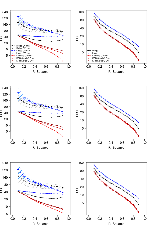
Figure 2: Estimation sum squared error (ESSE: left panels) and prediction sum squared errors (PSSE: right panels) of KPR (red), ridge regression (black) and lasso (blue), and their 95% confidence bands. We consider three sparsity settings for $\beta_{\mbox{\tiny True}}$, based on (3.1): $\|\beta_{\mbox{\tiny True}}\|_{0}=p$ in top panels; $\|\beta_{\mbox{\tiny True}}\|_{0}=\lfloor 0.6p\rfloor$ in center panels, and $\|\beta_{\mbox{\tiny True}}\|_{0}=\lfloor 0.2p\rfloor$ in bottom panels. For ridge and lasso, tuning parameters that produce the smallest cross-validated squared test error (CV min), and the largest tuning parameters such that the cross-validated squared test errors are within one standard error of the minimum cross-validated squared test error (CV 1se) are considered. For KPR, we consider $\|Q-Q_{obs}\|_{F}/\|Q\|_{F}=0$ (no $Q$ error), $0.25$ (small $Q$ error) and $0.5$ (large $Q$ error).

Figure 2 shows the estimation and prediction performance of KPR, ridge and lasso. KPR significantly outperforms both ridge regression and lasso for both prediction and estimation in all settings. As expected, the performance of ridge and lasso for estimation improve when using a larger tuning parameter. On the other hand, neither mis-specification of $Q$ nor sparsity of $\beta_{\mbox{\tiny True}}$ seems to substantially impact the relative performance of the three methods. This may be due to the fact that KPR estimates the correct target $\beta_{\mbox{\tiny True}}$, even with mis-specified $Q$, whereas ridge regression and lasso estimate the wrong target.

3.2 Regression and PCoA with respect to a UniFrac kernel

In the case of PCoA with respect to a UniFrac matrix $\Delta^{U}$ of squared dissimilarities, the graphical displays are based on the eigen-decomposition of $H=-\frac{1}{2}\mathcal{J}\Delta^{U}\mathcal{J}$. That is, for $H=U^{H}(S^{H})^{2}(U^{H})^{\prime}\approx U^{H}_{(2)}(S^{H}_{(2)})^{2}(U^{H}_{(2)})^{\prime}$, the $n$ samples are represented in two dimensions by the columns of $U^{H}_{(2)}S^{H}_{(2)}$; this results in points $\{\eta_{i1},\eta_{i2}\}_{i=1}^{n}:=\{(\sigma_{1}U^{H}_{i1},\sigma_{2}U^{H}_{i2})\}_{i=1}^{n}$, as plotted in Figure 1. When the points are colored according to a response variable, $\{y_{i}\}_{i=1}^{n}$, the implied regression model is

$$y =\gamma_{1}\eta_{1}+\gamma_{2}\eta_{2}+\epsilon$$ (3.2)

$$=U^{H}_{(2)}S^{H}_{(2)}\,\gamma+\epsilon.$$

However, in contrast to PCR in eq. (2.2), where $US=XV$, it is not obvious how to connect $\gamma$ directly to the $p$-coordinates corresponding to the $p$ columns of $X$. Here, we exploit the joint eigenstructure of kernels $K_{I}$ and $H$ (see (2.13)) by proceeding as in (2.11) to obtain the estimate $\hat{\beta}_{H}=X^{\prime}\hat{\gamma}$ as in (2.14), with $Q=I$.

In this example, we use the same data as in Section 3.1. For KPR, we use $K=XX^{\prime}$ and obtain $H=-\frac{1}{2}\mathcal{J}\Delta^{U}\mathcal{J}$ using the UniFrac distance matrix. We simulate $\gamma_{\mbox{\tiny True}}$ and $y_{\mbox{\tiny True}}$ from the first two eigenvectors of $H$, as in (3.2):

$$\gamma_{\mbox{\tiny True}} =\left((U^{H}_{(2)})^{\prime}(S^{H}_{(2)})^{2}U^{H}_{(2)}\right)^{-1}S^{H}_{(2)}(U^{H}_{(2)})^{\prime}y$$

$$y_{\mbox{\tiny True}} =U^{H}_{(2)}S^{H}_{(2)}\gamma_{\mbox{\tiny True}}.$$

This bivariate regression is illustrated in Figure 1(b).

The simulation is repeated 500 times, each with a different $\epsilon\sim N_{n}(0,\sigma^{2}_{\epsilon}I_{n})$ to produce various values of $R^{2}\in\{0.1,0.2,\ldots,0.9\}$. We compute $\hat{y}_{\mbox{\tiny KPR}}=K\hat{\gamma}_{\mbox{\tiny KPR}}$, where $\hat{\gamma}_{\mbox{\tiny KPR}}$ is estimated using (2.10). Similar to the last example, we do not assume we always observe the $H$ matrix that is used to generate $\gamma_{\mbox{\tiny True}}$ and $y_{\mbox{\tiny True}}$; rather, we use a noisy version, $H_{obs}$, of $H$ in KPR with $\|H-H_{obs}\|_{F}/\|H\|_{F}\in\{0,0.25,0.5\}$.

Since there is no meaningful way to simulate $\beta_{\mbox{\tiny True}}$, we do not compare the methods based on their estimation performances, and only consider prediction. For all three methods, we find the tuning parameters that minimize the cross-validated $H_{obs}$-weighted squared test error. While the use of $H$ in tuning ridge and lasso penalties deviates from the common practice, it results in improved performances, given the important role of $H$ in this simulation. The $H$ matrix also defines the valid distance in this example. Thus, to evaluate the prediction performances of various methods, we use the $H$-weighted prediction sum of squared error (HPSSE), $\|\hat{y}-y_{\mbox{\tiny True}}\|^{2}_{H}$.

Figure 3 shows that KPR consistently outperforms ridge regression and lasso in prediction, even with a reasonable amount of misspecification of $H$. This may be due to the fact that, with the incorporation of the $H$ matrix, KPR estimates the correct target whereas ridge and lasso do not.

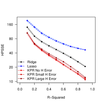
Figure 3: $H$-weighted prediction sum of squared error (HPSSE) of KPR (red), ridge (black) and lasso (blue), with 95% confidence bands. For KPR, we consider $\|H-H_{obs}\|_{F}/\|H\|_{F}=0$ (no $H$ Error), $0.25$ (small $H$ Error) and $0.5$ (large $H$ Error).

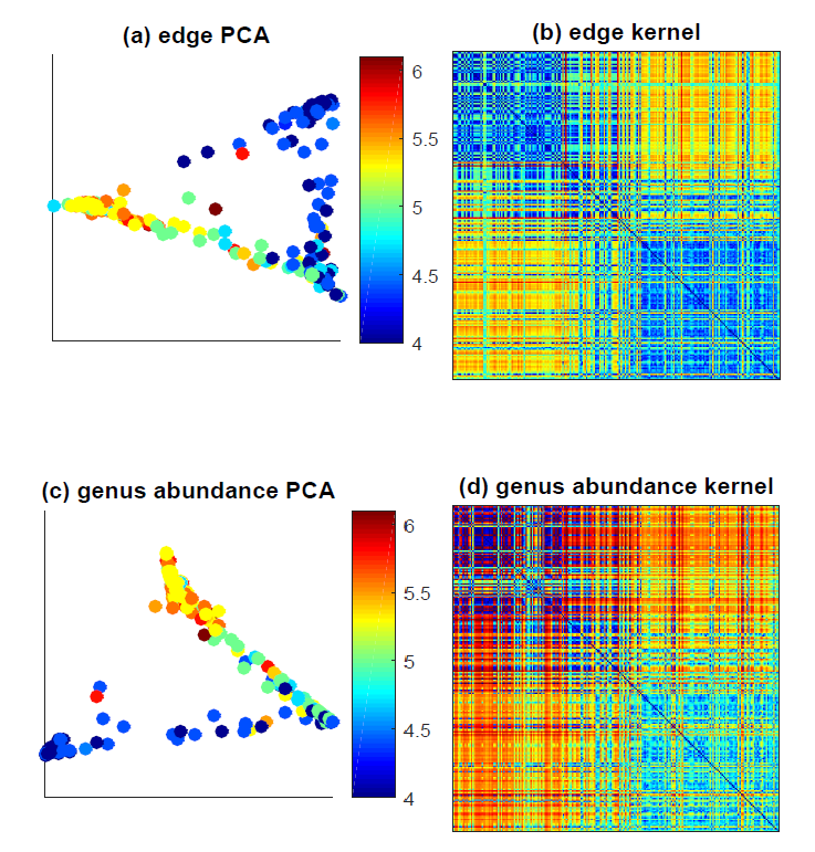
Figure 4: Analysis of bacterial vaginosis data from Srinivasan et al. (2012). (a): representation of the samples in the space of the first two PC’s of the edge-matrix kernel $H=EE^{\prime}$. The color of each point corresponds to the pH level of the sample; (b): heatmap of edge-matrix kernel used to generate the plot in (a); (c): two-dimensional PCA plot based on the genus-level relative abundances; (d): heatmap of the genus-abundance kernel $K=XX^{\prime}$ used to create the plot in (c). In (b) and (d), subjects are ordered by the pH values.

3.3 Regression and PCoA using an edge-matrix kernel

In this section, simulations are based on data from a study of bacterial vaginosis (BV) by Srinivasan et al. (2012) in which 16S rRNA gene samples were collected using vaginal swabs from $n=220$ women with and without BV. Here, the outcome $y$ represents pH measured from vaginal fluid of each subject and we consider the association of $y$ with genus-level taxa. In this example, we use the $p=62$ genera that exhibit non-zero sequence counts in at least 20% of the subjects. So here, $X$ represents $220\times 62$ abundances in a sample-by-genus matrix, and we use a kernel $K=XX^{\prime}$. Additionally, however, we define a second kernel $H=EE^{\prime}$ based on the “edge mass difference matrix”, $E$, originally introduced by Matsen and Evans (2013). If the full phylogenetic tree has $q$ edges, each sample can be represented by a vector indexed by all $q$ edges, the $e^{\text{th}}$ coordinate of which quantifies the difference between the fraction of sequence reads on either side of the edge; i.e., the fraction of reads observed on the root side of the tree minus the fraction of reads on the non-root side. We refer to Matsen and Evans (2013) for details and a discussion of “edge PCA”, which refers to PCA applied to the $n\times q$ matrix $E$. Note, in particular, that abundances from every taxon level in the tree contribute to a similarity between subjects as opposed to abundances at a single taxon level, which is used in UniFrac or DPCoA.

In summary, $X$ represents $p=62$ genus-level abundances while $E$ is based on all $q=1770$ edges in the original phylogenetic tree. Figure 4(a) shows a PCA plot of the 220 subjects in which their similarity is defined using the edge kernel $H=EE^{\prime}$; the color of each dot represents the subject’s pH. Figure 4(b) is a heatmap of the kernel $H$ used to create Figure 4(a). The columns and rows of $H$ represent similarities between samples based on the edge mass difference matrix, ordered by subject pH measurement. Similarly, Figure 4(c) is a PCA plot based on similarities defined using the genus-level abundance kernel, $K=XX^{\prime}$. Figure 4(d) is a heatmap of the kernel $K$ used to create Figure 4(c), and subjects are again ordered by pH. These figures illustrate how two different measures of similarity (two separate kernels) may be co-informative in the sense that they both provide information about grouping of subjects’ microbiota in relation to their pH. It is thus natural to expect that incorporating information from both $H$ and $K$ within the KPR framework may result in improved estimates of association between $y=\mbox{pH}$ and the taxon abundances.

For the simulation, we define a “true” association between pH and the genus-level taxa in $X$ using the 2-dimensional PCR model in eq. (2.2) and (2.3). Specifically, we use the apparent association between $y=\mbox{pH}$ and genus-level abundances in Figure 4(c) to construct a “true” coefficient vector $\beta_{\mbox{\tiny True}}$ as follows. Using the SVD of $X$, $X=USV^{\prime}$, set

$$y_{\mbox{\tiny True}}=U_{(2)}S_{(2)}\left(U^{\prime}_{(2)}S_{(2)}^{2}U_{(2)}\right)^{-1}S_{(2)}U^{\prime}_{(2)}y;$$

then project $y_{\mbox{\tiny True}}$ onto the space spanned by the first two singular vectors

$$\beta_{\mbox{\tiny True}}=V_{(2)}S_{(2)}^{-1}U_{(2)}^{\prime}y_{\mbox{\tiny True}}.$$

Taking $H=EE^{\prime}$ in a KPR model of the form (2.10), we compare the resulting estimate of $\beta$ with ridge and lasso estimates. (Note that $y_{\mbox{\tiny True}}$ and $\beta_{\mbox{\tiny True}}$ are not informed by $E$.) The simulation is repeated 500 times, each with a different $\epsilon\sim N_{n}(0,\sigma^{2}_{\epsilon}I_{n})$ to produce various values of $R^{2}\in\{0.1,0.2,...,0.9\}$. The performance metrics are the estimation sum squared error (ESSE) the $H$-weighted prediction sum squared error (HPSSE) as in the previous section. In this numerical example, we do not assume we always observe the true $H$ matrix; rather, we use a noisy version, $H_{obs}$, of $H$ in KPR with $\|H-H_{obs}\|_{F}/\|H\|_{F}\in\{0,0.25,0.5\}$. For all three methods, tuning parameter values are chosen to minimize the sum of squared test error weighted by $H_{obs}$. As in the simulation for DPCoA, we also allow for using the largest tuning parameters such that the squared test error weighted by $H$ is within one standard error of the minimum squared test error.

Figure 5 shows that KPR significantly outperforms ridge and lasso in both prediction and estimation. Note that even though $H$ is not used to simulate the true association, the use of edge kernel in KPR enhances the performance of both estimation and prediction, as long as $H$ is not severely misspecified. Once again, the performance of estimates from ridge and lasso improve when using a larger tuning parameter (CV 1se).

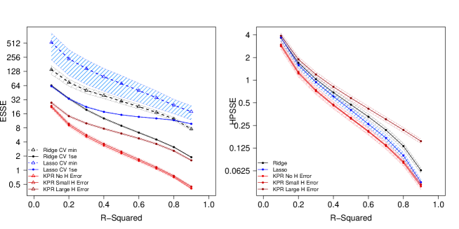
Figure 5: In silico evaluation of using tree-based edge information in regression models. Estimation sum squared error (ESSE) and $H$-weighted prediction sum squared error (HPSSE) of KPR (red), ridge regression (black) and lasso (blue), with the 95% confidence bands. For KPR, we consider $\|H-H_{obs}\|_{F}/\|H\|_{F}=0$ (no $H$ error), $0.25$ (small $H$ error) and $0.5$ (large $H$ error).

4 Application to an observational study

We apply our kernel-penalized regression framework to data from 16S rRNA gene collected in a study of premenopausal women (Hullar et al., 2015). This study investigated aspects of gut microbial communities in stool samples from premenopausal women using 454 pyrosequencing of the 16S rRNA gene. The abundances of 127 species were zero for more than 90% of the subjects and were removed from our analysis. The data set we consider consists of $p=128$ species sampled from $n=102$ women.

To make the measurements comparable between subjects, the species abundances were scaled by the total number of sequences measured in each sample. This scaling produces compositional data (the relative abundances in each sample sum to 1) which introduces analytical complications. In particular, regression analysis using compositional covariates must somehow account for their unit sum constraint (Kurtz et al., 2015; Li, 2015). For this reason, we apply the CLR transformation to the relative abundance values and use this transformed data $\tilde{X}$ as the matrix of predictors in the KPR model. Additionally, using Aitchison’s variation matrix (Aitchison, 1982), $T$, we obtain the covariance matrix, $C$, as described prior to eq. (2.15). As $C$ provides more accurate information on the covariance among the true abundances than does the empirical covariance matrix from relative abundances, $X$, or their CLR transform, $\tilde{X}$, we use $C$ in place of $Q$ in (2.5).

In this example, we examine the effect of using the CLR transformed data $\tilde{X}$ and covariance $C$ as in (2.15) and fit penalized regression models with the goal of estimating $\tilde{\beta}_{C}$ in (2.15) for the purpose of identifying specific species that may be associated with percent fat in the cohort described above. To this end, we apply a recently developed significance testing procedure to three high-dimensional models in order to identify species exhibiting evidence of association with subjects’ adiposity. This significance test for graph-constrained estimation, called Grace (Zhao and Shojaie, 2016), provides a means to assign significance to estimates from penalized regression models that incorporate structure of the type provided by $Q$ in (2.5) (or $C$ in (2.15)). The method asymptotically controls the type-I error rate regardless of the choice of $Q$. The special case with $Q=I$ provides a significance test for ordinary ridge regression. In each application of the Grace test, tuning parameters are selected based on the smallest squared test error using 10-fold cross validation. Following Zhao and Shojaie (2016), the assumed sparsity parameter is set to be $\xi=0.05$. The tuning parameter for the initial estimator is set to be $\lambda_{init}=4\hat{\sigma}_{\epsilon}\sqrt{3\log p/n}$, where $\hat{\sigma}_{\epsilon}$ is the estimated standard deviation of the random error $\epsilon$, using the scaled Lasso (Sun and Zhang, 2012). To assess significance for the sparse models using lasso, we apply the recently proposed significance test for lasso regressions based on low-dimensional projection estimator (LDPE) (Zhang and Zhang, 2014; Van de Geer et al., 2014), which provides an asymptotically valid test for lasso-penalized regression estimates.

Table 1: Species found to be associated with percent fat (in increasing order of p-values) at different significant levels using: KPR with centered log-ratio transformed abundances (CLR) ; ridge and lasso regression with centered log-ratio transformed abundances; and ridge and lasso regression with untransformed relative abundances (rel%).

	$p<0.01$	$p<0.005$	FDR $<0.1$
KPR $+$ CLR	Bacteroides, Anaerovorax, Acidaminococcus, Blautia, Dethiosulfatibacter, Asaccharobacter, Turicibacter, Lebetimonas, Streptobacillus, Anoxynatronum	Bacteroides, Turicibacter, Acidaminococcus, Dethiosulfatibacter	(none)
Ridge $+$ CLR	(none)	(none)	(none)
Ridge $+$ rel%	Catonella, Dethiosulfatibacter	(none)	(none)
Lasso $+$ CLR	Roseburia	(none)	(none)
Lasso $+$ rel%	Dethiosulfatibacter, Micropruina	Dethiosulfatibacter	(none)

We report on five regression estimation methods for which the significance of regression coefficients can be evaluated using existing high-dimensional testing methods. Two are obtained using the relative abundances, $X$, with respect to: (i) an ordinary ridge penalty and (ii) a lasso penalty. Three are obtained using the CLR transformed abundances, $\tilde{X}$, with respect to: (iii) an ordinary ridge penalty, (iv) a lasso penalty, and (v) the KPR estimate in (2.15). None of these methods result in any species associated with the outcome of percent fat when controlled for false discovery rate (FDR) at 0.1 using the Benjamini-Yekutieli procedure (Benjamini and Yekutieli, 2001). However, when using a cut-off of $p=0.01$, the KPR estimate (2.15) results in ten species. With a cut-off of $p=0.005$, KPR results in four species. Ordinary ridge regressions using the CLR-transformed vectors find no associations at a cut-off of $p=0.01$, whereas using the relative abundances, ridge finds two species at the $p=0.01$ cut-off and none at $p=0.005$. Lasso regression with the CLR-transformed vectors identifies one specie at the $p=0.01$ cut-off and none at $p=0.005$ cut-off. When using the relative abundances, lasso identifies two species as significant at the $p=0.01$ cut-off and one at the $p=0.005$ cutoff. See Table 1 for the list of identified species.

5 Discussion

We have formulated a family of regression models that naturally extends the dimension-reduced graphical explorations common to microbiome studies. In this sense, we have simply re-focused the role of the eigen-structures used in ordination methods toward exploiting this structure in penalized regression models. The large family of models developed here provides a supervised statistical learning counterpart to the unsupervised methods of principal coordinate analysis (PCoA).

A primary motivations for PCoA graphical displays is the ability to incorporate biologically-inclined measures of (dis)similarity. The popular use of UniFrac, for instance, is motivated by the desire to impose phylogeny into the analysis. These dissimilarities have also been used for rigorous statistical testing in the context of Anderson’s nonparametric MANOVA (Anderson, 2006) or the closely-related kernel machine regression score test (Chen et al., 2012; Pan, 2011; Zhao et al., 2015) for global association of a multivariate predictor with an outcome. However, the use of UniFrac and other non-Euclidean distances make it difficult to identify specific associations between the microbial abundance profiles and a phenotype; indeed, none of these analyses proceed to estimate the individual associations. In addition to ordination displays and global tests for associations, a variety of machine learning approaches have emphasized on models that predict a response. In contrast, we focus on estimating the coefficient vector, which is a key aspect of any approach used to draw scientific conclusions based on the association of microbial communities with an outcome or phenotype.

An interesting feature of the proposed kernel-penalized regression framework is its ability to sidestep some of the problems inherent in compositional data analysis. Indeed, as emphasized by Li (2015) regression analysis with compositional covariates must somehow acknowledge their unit-sum constraint and spurious correlations. Our approach, which differs somewhat from that of Li (2015), may also be viewed as a penalized version of the low-dimensional linear model for compositions by Tolosana-Delgado and Van Den Boogart (2011), who use the isometric log-ratio (ILR) coordinates. We note that ILR coordinates arise from the SVD of mean-centered CLR-transformed data, $\tilde{X}$ (see Egozcue and Pawlowsky-Glahn (2011)), which is also used in our model. However, to estimate $\beta\in\mathbb{R}^{p}$, we used instead a regularization framework; our penalty in Section 2.4 arises from Aithison’s total variation matrix whose singular values are the total variances of ILR components. Moreover, the proposed framework also allows us to use existing inference frameworks for high-dimensional regression, and in particular the Grace test (Zhao and Shojaie, 2016), to assess the significance of estimated regression coefficients.

References

- Aitchison (1982) {barticle}[author] \bauthor\bsnmAitchison, \bfnmJ.\binitsJ. (\byear1982). \btitleThe Statistical Analysis of Compositional Data. \bjournalJournal of the Royal Statistical Society: Series B \bvolume44 \bpages139-177. \endbibitem
- Aitchison (2003a) {binproceedings}[author] \bauthor\bsnmAitchison, \bfnmJ.\binitsJ. (\byear2003a). \btitleA concise guide to compositional data analysis. In \bbooktitle2nd Compositional Data Analysis Workshop. \endbibitem
- Aitchison (2003b) {bbook}[author] \bauthor\bsnmAitchison, \bfnmJ.\binitsJ. (\byear2003b). \btitleThe Statistical Analysis of Compositional Data. \bpublisherThe Blackburn Press, \baddressCaldwell, NJ. \endbibitem
- Anderson (2006) {barticle}[author] \bauthor\bsnmAnderson, \bfnmM. J.\binitsM. J. (\byear2006). \btitleDistance-Based Tests for Homogeneity of Multivariate Dispersions. \bjournalBiometrics \bvolume62 \bpages245-253. \endbibitem
- Benjamini and Yekutieli (2001) {barticle}[author] \bauthor\bsnmBenjamini, \bfnmY.\binitsY. and \bauthor\bsnmYekutieli, \bfnmD.\binitsD. (\byear2001). \btitleThe control of the false discovery rate in multiple testing under dependency. \bjournalThe Annals of Statistics \bvolume29 \bpages1165-1188. \endbibitem
- Bühlmann, Kalisch and Meier (2014) {barticle}[author] \bauthor\bsnmBühlmann, \bfnmP.\binitsP., \bauthor\bsnmKalisch, \bfnmM.\binitsM. and \bauthor\bsnmMeier, \bfnmL.\binitsL. (\byear2014). \btitleHigh-Dimensional Statistics with a View Toward Applications in Biology. \bjournalAnnual Review of Statistics and Its Application \bvolume1 \bpages255-278. \endbibitem
- Cai and Hall (2006) {barticle}[author] \bauthor\bsnmCai, \bfnmT. T.\binitsT. T. and \bauthor\bsnmHall, \bfnmP.\binitsP. (\byear2006). \btitlePrediction in functional linear regression. \bjournalThe Annals of Statistics \bvolume34 \bpages2159-2179. \endbibitem
- Chen et al. (2012) {barticle}[author] \bauthor\bsnmChen, \bfnmJ.\binitsJ., \bauthor\bsnmBittinger, \bfnmK.\binitsK., \bauthor\bsnmCharlson, \bfnmE. S.\binitsE. S., \bauthor\bsnmHoffmann, \bfnmC.\binitsC., \bauthor\bsnmLewis, \bfnmJ.\binitsJ., \bauthor\bsnmWu, \bfnmG. D.\binitsG. D., \bauthor\bsnmCollman, \bfnmR. G.\binitsR. G., \bauthor\bsnmBushman, \bfnmF. D.\binitsF. D. and \bauthor\bsnmLi, \bfnmH.\binitsH. (\byear2012). \btitleAssociating microbiome composition with environmental covariates using generalized UniFrac distances. \bjournalBioinformatics \bvolume28 \bpages2106-2113. \endbibitem
- Claesson et al. (2012) {barticle}[author] \bauthor\bsnmClaesson, \bfnmM. J.\binitsM. J., \bauthor\bsnmJeffery, \bfnmI. B.\binitsI. B., \bauthor\bsnmConde, \bfnmS.\binitsS., \bauthor\bsnmPower, \bfnmS. E.\binitsS. E., \bauthor\bsnmO’Connor, \bfnmE. M.\binitsE. M., \bauthor\bsnmCusack, \bfnmS.\binitsS., \bauthor\bsnmHarris, \bfnmH. M.\binitsH. M., \bauthor\bsnmCoakley, \bfnmM.\binitsM., \bauthor\bsnmLakshminarayanan, \bfnmB.\binitsB., \bauthor\bsnmO’Sullivan, \bfnmO.\binitsO., \bauthor\bsnmFitzgerald, \bfnmG. F.\binitsG. F., \bauthor\bsnmDeane, \bfnmJ.\binitsJ., \bauthor\bsnmO’Connor, \bfnmM.\binitsM., \bauthor\bsnmHarnedy, \bfnmN.\binitsN., \bauthor\bsnmO’Connor, \bfnmK.\binitsK., \bauthor\bsnmO’Mahony, \bfnmD.\binitsD., \bauthor\bparticlevan \bsnmSinderen, \bfnmD.\binitsD., \bauthor\bsnmWallace, \bfnmM.\binitsM., \bauthor\bsnmBrennan, \bfnmL.\binitsL., \bauthor\bsnmStanton, \bfnmC.\binitsC., \bauthor\bsnmMarchesi, \bfnmJ. R.\binitsJ. R., \bauthor\bsnmFitzgerald, \bfnmA. P.\binitsA. P., \bauthor\bsnmShanahan, \bfnmF.\binitsF., \bauthor\bsnmHill, \bfnmC.\binitsC., \bauthor\bsnmRoss, \bfnmR. P.\binitsR. P. and \bauthor\bsnmO’Toole, \bfnmP. W.\binitsP. W. (\byear2012). \btitleGut microbiota composition correlates with diet and health in the elderly. \bjournalNature \bvolume488 \bpages178-184. \endbibitem
- The Human Microbiome Project Consortium (2012) {barticle}[author] \bauthor\bsnmThe Human Microbiome Project Consortium (\byear2012). \btitleStructure, function and diversity of the healthy human microbiome. \bjournalNature \bvolume486 \bpages207-214. \endbibitem
- Egozcue and Pawlowsky-Glahn (2011) {bincollection}[author] \bauthor\bsnmEgozcue, \bfnmJ. J.\binitsJ. J. and \bauthor\bsnmPawlowsky-Glahn, \bfnmV.\binitsV. (\byear2011). \btitleBasic Concepts and Procedures. In \bbooktitleCompositional Data Analysis: Theory and Applications (\beditor\bfnmV.\binitsV. \bsnmPawlowsky-Glahn and \beditor\bfnmA.\binitsA. \bsnmBuccianti, eds.) \bchapter2, \bpages12-28. \bpublisherJohn Wiley & Sons, \baddressChichester, West Sussex, UK. \endbibitem
- Evans and Matsen (2012) {barticle}[author] \bauthor\bsnmEvans, \bfnmS. N.\binitsS. N. and \bauthor\bsnmMatsen, \bfnmF. A.\binitsF. A. (\byear2012). \btitleThe phylogenetic Kantorovich–Rubinstein metric for environmental sequence samples. \bjournalJournal of the Royal Statistical Society: Series B \bvolume74 \bpages569-592. \endbibitem
- Franklin (1978) {barticle}[author] \bauthor\bsnmFranklin, \bfnmJ. N.\binitsJ. N. (\byear1978). \btitleMinimum principles for ill-posed problems. \bjournalSIAM Journal on Mathematical Analysis \bvolume9 \bpages638-650. \endbibitem
- Freytag et al. (2014) {barticle}[author] \bauthor\bsnmFreytag, \bfnmS.\binitsS., \bauthor\bsnmManitz, \bfnmJ.\binitsJ., \bauthor\bsnmSchlather, \bfnmM.\binitsM., \bauthor\bsnmKneib, \bfnmT.\binitsT., \bauthor\bsnmAmos, \bfnmC. I.\binitsC. I., \bauthor\bsnmRisch, \bfnmA.\binitsA., \bauthor\bsnmChang-Claude, \bfnmJ.\binitsJ., \bauthor\bsnmHeinrich, \bfnmJ.\binitsJ. and \bauthor\bsnmBickeböller, \bfnmH.\binitsH. (\byear2014). \btitleA network-based kernel machine test for the identification of risk pathways in genome-wide association studies. \bjournalHuman heredity \bvolume76 \bpages64-75. \endbibitem
- Friedman and Alm (2012) {barticle}[author] \bauthor\bsnmFriedman, \bfnmJ.\binitsJ. and \bauthor\bsnmAlm, \bfnmE. J.\binitsE. J. (\byear2012). \btitleInferring correlation networks from genomic survey data. \bjournalPLoS Computational Biology \bvolume8 \bpagese1002687. \endbibitem
- Fukuyama et al. (2012) {binproceedings}[author] \bauthor\bsnmFukuyama, \bfnmJ.\binitsJ., \bauthor\bsnmMcMurdie, \bfnmP. J.\binitsP. J., \bauthor\bsnmDethlefsen, \bfnmL.\binitsL., \bauthor\bsnmRelman, \bfnmD. A.\binitsD. A. and \bauthor\bsnmHolmes, \bfnmS.\binitsS. (\byear2012). \btitleComparisons of distance methods for combining covariates and abundances in microbiome studies. In \bbooktitlePacific Symposium on Biocomputing \bvolume17 \bpages213-224. \endbibitem
- Golub and van Loan (2012) {bbook}[author] \bauthor\bsnmGolub, \bfnmG. h.\binitsG. h. and \bauthor\bparticlevan \bsnmLoan, \bfnmC. F.\binitsC. F. (\byear2012). \btitleMatrix Computations. \bseriesJohns Hopkins Studies in the Mathematical Sciences. \bpublisherJohns Hopkins University Press, \baddressBaltimore, MD. \endbibitem
- Goodrich et al. (2014) {barticle}[author] \bauthor\bsnmGoodrich, \bfnmJ. K.\binitsJ. K., \bauthor\bsnmDi Rienzi, \bfnmS. C.\binitsS. C., \bauthor\bsnmPoole, \bfnmA. C.\binitsA. C., \bauthor\bsnmKoren, \bfnmO.\binitsO., \bauthor\bsnmWalters, \bfnmW. A.\binitsW. A., \bauthor\bsnmCaporaso, \bfnmJ. G.\binitsJ. G., \bauthor\bsnmKnight, \bfnmR.\binitsR. and \bauthor\bsnmLey, \bfnmR. E.\binitsR. E. (\byear2014). \btitleConducting a microbiome study. \bjournalCell \bvolume158 \bpages250-262. \endbibitem
- Gower (1966) {barticle}[author] \bauthor\bsnmGower, \bfnmJ. C.\binitsJ. C. (\byear1966). \btitleSome distance properties of latent root and vector methods used in multivariate analysis. \bjournalBiometrika \bvolume53 \bpages325-338. \endbibitem
- Greenacre (1984) {bbook}[author] \bauthor\bsnmGreenacre, \bfnmM. J.\binitsM. J. (\byear1984). \btitleTheory and Applications of Correspondence Analysis. \bpublisherAcademic Press, \baddressCambridge, MA. \endbibitem
- Gretton et al. (2005) {barticle}[author] \bauthor\bsnmGretton, \bfnmA.\binitsA., \bauthor\bsnmHerbrich, \bfnmR.\binitsR., \bauthor\bsnmSmola, \bfnmA.\binitsA., \bauthor\bsnmBousquet, \bfnmO.\binitsO. and \bauthor\bsnmSchölkopf, \bfnmB.\binitsB. (\byear2005). \btitleKernel methods for measuring independence. \bjournalThe Journal of Machine Learning Research \bvolume6 \bpages2075-2129. \endbibitem
- Hamady and Knight (2009) {barticle}[author] \bauthor\bsnmHamady, \bfnmM.\binitsM. and \bauthor\bsnmKnight, \bfnmR.\binitsR. (\byear2009). \btitleMicrobial community profiling for human microbiome projects: Tools, techniques, and challenges. \bjournalGenome Research \bvolume19 \bpages1141-1152. \endbibitem
- Hansen (1998) {bbook}[author] \bauthor\bsnmHansen, \bfnmP. C.\binitsP. C. (\byear1998). \btitleRank-Deficient and Discrete ill-Posed Problems: Numerical Aspects of Linear Inversion. \bpublisherSIAM, \baddressPhiladelphia, PA. \endbibitem
- Hastie, Tibshirani and Friedman (2009) {bbook}[author] \bauthor\bsnmHastie, \bfnmT.\binitsT., \bauthor\bsnmTibshirani, \bfnmR.\binitsR. and \bauthor\bsnmFriedman, \bfnmJ.\binitsJ. (\byear2009). \btitleThe Elements of Statistical Learning: Data Mining, Inference, and Prediction. \bseriesSpringer Series in Statistics. \bpublisherSpringer-Verlag, \baddressNew York, NY. \endbibitem
- Hoerl and Kennard (1970) {barticle}[author] \bauthor\bsnmHoerl, \bfnmA. E.\binitsA. E. and \bauthor\bsnmKennard, \bfnmR. W.\binitsR. W. (\byear1970). \btitleRidge Regression: Biased Estimation for Nonorthogonal Problems. \bjournalTechnometrics \bvolume12 \bpages55-67. \endbibitem
- Hullar et al. (2015) {barticle}[author] \bauthor\bsnmHullar, \bfnmM. A.\binitsM. A., \bauthor\bsnmLancaster, \bfnmS. M.\binitsS. M., \bauthor\bsnmLi, \bfnmF.\binitsF., \bauthor\bsnmTseng, \bfnmE.\binitsE., \bauthor\bsnmBeer, \bfnmK.\binitsK., \bauthor\bsnmAtkinson, \bfnmC.\binitsC., \bauthor\bsnmWähälä, \bfnmK.\binitsK., \bauthor\bsnmCopeland, \bfnmW. K.\binitsW. K., \bauthor\bsnmRandolph, \bfnmT. W.\binitsT. W., \bauthor\bsnmNewton, \bfnmK. M.\binitsK. M. and \bauthor\bsnmLampe, \bfnmJ. W.\binitsJ. W. (\byear2015). \btitleEnterolignan-Producing Phenotypes Are Associated with Increased Gut Microbial Diversity and Altered Composition in Premenopausal Women in the United States. \bjournalCancer Epidemiology Biomarkers & Prevention \bvolume24 \bpages546-554. \endbibitem
- Josse and Holmes (2014) {barticle}[author] \bauthor\bsnmJosse, \bfnmJ.\binitsJ. and \bauthor\bsnmHolmes, \bfnmS.\binitsS. (\byear2014). \btitleTests of independence and beyond. Literature review. \bjournalarXiv preprint arXiv:1307.7383v3. \endbibitem
- Kim and Xing (2010) {binproceedings}[author] \bauthor\bsnmKim, \bfnmS.\binitsS. and \bauthor\bsnmXing, \bfnmE. P.\binitsE. P. (\byear2010). \btitleTree-guided group lasso for multi-task regression with structured sparsity. In \bbooktitleProceedings of the 27th International Conference on Machine Learning (ICML 2010) (\beditor\bfnmJ.\binitsJ. \bsnmFürnkranz and \beditor\bfnmT.\binitsT. \bsnmJoachims, eds.) \bpages543-550. \endbibitem
- Koren et al. (2013) {barticle}[author] \bauthor\bsnmKoren, \bfnmO.\binitsO., \bauthor\bsnmKnights, \bfnmD.\binitsD., \bauthor\bsnmGonzalez, \bfnmA.\binitsA., \bauthor\bsnmWaldron, \bfnmL.\binitsL., \bauthor\bsnmSegata, \bfnmN.\binitsN., \bauthor\bsnmKnight, \bfnmR.\binitsR., \bauthor\bsnmHuttenhower, \bfnmC.\binitsC. and \bauthor\bsnmLey, \bfnmR. E.\binitsR. E. (\byear2013). \btitleA guide to enterotypes across the human body: meta-analysis of microbial community structures in human microbiome datasets. \bjournalPLoS Computational Biology \bvolume9 \bpagese1002863. \endbibitem
- Kuczynski et al. (2010) {barticle}[author] \bauthor\bsnmKuczynski, \bfnmJ.\binitsJ., \bauthor\bsnmLiu, \bfnmZ.\binitsZ., \bauthor\bsnmLozupone, \bfnmC.\binitsC., \bauthor\bsnmMcDonald, \bfnmD.\binitsD., \bauthor\bsnmFierer, \bfnmN.\binitsN. and \bauthor\bsnmKnight, \bfnmR.\binitsR. (\byear2010). \btitleMicrobial community resemblance methods differ in their ability to detect biologically relevant patterns. \bjournalNature Methods \bvolume7 \bpages813-819. \endbibitem
- Kurtz et al. (2015) {barticle}[author] \bauthor\bsnmKurtz, \bfnmZ. D.\binitsZ. D., \bauthor\bsnmMueller, \bfnmC. L.\binitsC. L., \bauthor\bsnmMiraldi, \bfnmE. R.\binitsE. R., \bauthor\bsnmLittman, \bfnmD. R.\binitsD. R., \bauthor\bsnmBlaser, \bfnmM. J.\binitsM. J. and \bauthor\bsnmBonneau, \bfnmR. A.\binitsR. A. (\byear2015). \btitleSparse and compositionally robust inference of microbial ecological networks. \bjournalPLoS Computational Biology \bvolume11 \bpagese1004226. \endbibitem
- Li (2015) {barticle}[author] \bauthor\bsnmLi, \bfnmH.\binitsH. (\byear2015). \btitleMicrobiome, Metagenomics, and High-Dimensional Compositional Data Analysis. \bjournalAnnual Review of Statistics and Its Application \bvolume2 \bpages73-94. \endbibitem
- Li and Li (2008) {barticle}[author] \bauthor\bsnmLi, \bfnmC.\binitsC. and \bauthor\bsnmLi, \bfnmH.\binitsH. (\byear2008). \btitleNetwork-constrained regularization and variable selection for analysis of genomic data. \bjournalBioinformatics \bvolume24 \bpages1175-1182. \endbibitem
- Lovell et al. (2015) {barticle}[author] \bauthor\bsnmLovell, \bfnmDavid\binitsD., \bauthor\bsnmPawlowsky-Glahn, \bfnmVera\binitsV., \bauthor\bsnmEgozcue, \bfnmJuan José\binitsJ. J., \bauthor\bsnmMarguerat, \bfnmSamuel\binitsS. and \bauthor\bsnmBähler, \bfnmJürg\binitsJ. (\byear2015). \btitleProportionality: a valid alternative to correlation for relative data. \bjournalPLoS computational biology \bvolume11 \bpagese1004075. \endbibitem
- Lozupone and Knight (2005) {barticle}[author] \bauthor\bsnmLozupone, \bfnmC.\binitsC. and \bauthor\bsnmKnight, \bfnmR.\binitsR. (\byear2005). \btitleUniFrac: a new phylogenetic method for comparing microbial communities. \bjournalApplied and environmental microbiology \bvolume71 \bpages8228–8235. \endbibitem
- Lozupone et al. (2007) {barticle}[author] \bauthor\bsnmLozupone, \bfnmC. A.\binitsC. A., \bauthor\bsnmHamady, \bfnmM.\binitsM., \bauthor\bsnmKelley, \bfnmS. T.\binitsS. T. and \bauthor\bsnmKnight, \bfnmR.\binitsR. (\byear2007). \btitleQuantitative and qualitative diversity measures lead to different insights into factors that structure microbial communities. \bjournalApplied and environmental microbiology \bvolume73 \bpages1576–1585. \endbibitem
- Mardia, Kent and Bibby (1980) {bbook}[author] \bauthor\bsnmMardia, \bfnmK. V.\binitsK. V., \bauthor\bsnmKent, \bfnmJ. T.\binitsJ. T. and \bauthor\bsnmBibby, \bfnmJ. M.\binitsJ. M. (\byear1980). \btitleMultivariate analysis. \bpublisherAcademic press. \endbibitem
- Matsen and Evans (2013) {barticle}[author] \bauthor\bsnmMatsen, \bfnmF. A\binitsF. A. and \bauthor\bsnmEvans, \bfnmS. N.\binitsS. N. (\byear2013). \btitleEdge principal components and squash clustering: using the special structure of phylogenetic placement data for sample comparison. \bjournalPLoS ONE \bvolume8 \bpagese56859. \endbibitem
- Pan (2011) {barticle}[author] \bauthor\bsnmPan, \bfnmW.\binitsW. (\byear2011). \btitleRelationship between genomic distance-based regression and kernel machine regression for multi-marker association testing. \bjournalGenetic Epidemiology \bvolume35 \bpages211–216. \endbibitem
- Pavoine, Dufour and Chessel (2004) {barticle}[author] \bauthor\bsnmPavoine, \bfnmS.\binitsS., \bauthor\bsnmDufour, \bfnmA-B.\binitsA.-B. and \bauthor\bsnmChessel, \bfnmD.\binitsD. (\byear2004). \btitleFrom dissimilarities among species to dissimilarities among communities: a double principal coordinate analysis. \bjournalJournal of Theoretical Biology \bvolume228 \bpages523–537. \endbibitem
- Pearson (1896) {barticle}[author] \bauthor\bsnmPearson, \bfnmKarl\binitsK. (\byear1896). \btitleMathematical Contributions to the Theory of Evolution—On a Form of Spurious Correlation Which May Arise When Indices Are Used in the Measurement of Organs. \bjournalProceedings of the royal society of london \bvolume60 \bpages489–498. \endbibitem
- Pekalska, Paclik and Duin (2002) {barticle}[author] \bauthor\bsnmPekalska, \bfnmElzbieta\binitsE., \bauthor\bsnmPaclik, \bfnmPavel\binitsP. and \bauthor\bsnmDuin, \bfnmRobert PW\binitsR. P. (\byear2002). \btitleA generalized kernel approach to dissimilarity-based classification. \bjournalThe Journal of Machine Learning Research \bvolume2 \bpages175–211. \endbibitem
- Purdom (2011) {barticle}[author] \bauthor\bsnmPurdom, \bfnmE.\binitsE. (\byear2011). \btitleAnalysis of a data matrix and a graph: Metagenomic data and the phylogenetic tree. \bjournalThe Annals of Applied Statistics \bvolume5 \bpages2326–2358. \endbibitem
- Randolph, Harezlak and Feng (2012) {barticle}[author] \bauthor\bsnmRandolph, \bfnmT. W.\binitsT. W., \bauthor\bsnmHarezlak, \bfnmJ.\binitsJ. and \bauthor\bsnmFeng, \bfnmZ.\binitsZ. (\byear2012). \btitleStructured penalties for functional linear models—partially empirical eigenvectors for regression. \bjournalElectronic Journal of Statistics \bvolume6 \bpages323–353. \endbibitem
- Robert and Escoufier (1976) {barticle}[author] \bauthor\bsnmRobert, \bfnmP.\binitsP. and \bauthor\bsnmEscoufier, \bfnmY.\binitsY. (\byear1976). \btitleA Unifying Tool for Linear Multivariate Statistical Methods: The RV- Coefficient. \bjournalJournal of the Royal Statistical Society: Series C \bvolume25 \bpages257-265. \endbibitem
- Ruppert, Wand and Carroll (2003) {bbook}[author] \bauthor\bsnmRuppert, \bfnmD.\binitsD., \bauthor\bsnmWand, \bfnmM. P.\binitsM. P. and \bauthor\bsnmCarroll, \bfnmR. J.\binitsR. J. (\byear2003). \btitleSemiparametric Regression. \bpublisherCambridge University Press, \baddressNew York. \endbibitem
- Schaid (2010) {barticle}[author] \bauthor\bsnmSchaid, \bfnmD. J.\binitsD. J. (\byear2010). \btitleGenomic similarity and kernel methods I: advancements by building on mathematical and statistical foundations. \bjournalHuman heredity \bvolume70 \bpages109–131. \endbibitem
- Schifano et al. (2012) {barticle}[author] \bauthor\bsnmSchifano, \bfnmE. D.\binitsE. D., \bauthor\bsnmEpstein, \bfnmM. P.\binitsM. P., \bauthor\bsnmBielak, \bfnmL. F.\binitsL. F., \bauthor\bsnmJhun, \bfnmM. A.\binitsM. A., \bauthor\bsnmKardia, \bfnmS. L. R.\binitsS. L. R., \bauthor\bsnmPeyser, \bfnmP. A.\binitsP. A. and \bauthor\bsnmLin, \bfnmX.\binitsX. (\byear2012). \btitleSNP set association analysis for familial data. \bjournalGenetic epidemiology \bvolume36 \bpages797–810. \endbibitem
- Schölkopf and Smola (2002) {bbook}[author] \bauthor\bsnmSchölkopf, \bfnmB.\binitsB. and \bauthor\bsnmSmola, \bfnmA. J.\binitsA. J. (\byear2002). \btitleLearning with kernels: Support vector machines, regularization, optimization, and beyond. \bpublisherMIT Press, \baddressCambridge, MA. \endbibitem
- Srinivasan et al. (2012) {barticle}[author] \bauthor\bsnmSrinivasan, \bfnmSujatha\binitsS., \bauthor\bsnmHoffman, \bfnmNoah G\binitsN. G., \bauthor\bsnmMorgan, \bfnmMartin T\binitsM. T., \bauthor\bsnmMatsen, \bfnmFrederick A\binitsF. A., \bauthor\bsnmFiedler, \bfnmTina L\binitsT. L., \bauthor\bsnmHall, \bfnmRobert W\binitsR. W., \bauthor\bsnmRoss, \bfnmFrederick J\binitsF. J., \bauthor\bsnmMcCoy, \bfnmConnor O\binitsC. O., \bauthor\bsnmBumgarner, \bfnmRoger\binitsR., \bauthor\bsnmMarrazzo, \bfnmJeanne M\binitsJ. M. \betalet al. (\byear2012). \btitleBacterial communities in women with bacterial vaginosis: high resolution phylogenetic analyses reveal relationships of microbiota to clinical criteria. \bjournalPloS one \bvolume7 \bpagese37818. \endbibitem
- Sun and Zhang (2012) {barticle}[author] \bauthor\bsnmSun, \bfnmT.\binitsT. and \bauthor\bsnmZhang, \bfnmC. H.\binitsC. H. (\byear2012). \btitleScaled sparse linear regression. \bjournalBiometrika \bvolume99 \bpages879-898. \endbibitem
- Székely and Rizzo (2009) {barticle}[author] \bauthor\bsnmSzékely, \bfnmG. J.\binitsG. J. and \bauthor\bsnmRizzo, \bfnmM. L.\binitsM. L. (\byear2009). \btitleBrownian distance covariance. \bjournalThe Annals of Applied Statistics \bvolume3 \bpages1236–1265. \endbibitem
- Tanaseichuk, Borneman and Jiang (2014) {barticle}[author] \bauthor\bsnmTanaseichuk, \bfnmO.\binitsO., \bauthor\bsnmBorneman, \bfnmJ.\binitsJ. and \bauthor\bsnmJiang, \bfnmT.\binitsT. (\byear2014). \btitlePhylogeny-based classification of microbial communities. \bjournalBioinformatics \bvolume30 \bpages449-456. \endbibitem
- Tibshirani and Taylor (2011) {barticle}[author] \bauthor\bsnmTibshirani, \bfnmR. J.\binitsR. J. and \bauthor\bsnmTaylor, \bfnmJ\binitsJ. (\byear2011). \btitleThe solution path of the generalized lasso. \bjournalThe Annals of Statistics \bvolume39 \bpages1335–1371”. \endbibitem
- Tolosana-Delgado and Van Den Boogart (2011) {bincollection}[author] \bauthor\bsnmTolosana-Delgado, \bfnmV.\binitsV. and \bauthor\bsnmVan Den Boogart, \bfnmK. G.\binitsK. G. (\byear2011). \btitleLinear Models with Compositions in R. In \bbooktitleCompositional Data Analysis: Theory and Applications (\beditor\bfnmV.\binitsV. \bsnmPawlowsky-Glahn and \beditor\bfnmA.\binitsA. \bsnmBuccianti, eds.) \bchapter26, \bpages12-28. \bpublisherJohn Wiley & Sons, \baddressChichester, West Sussex, UK. \endbibitem
- Van de Geer et al. (2014) {barticle}[author] \bauthor\bparticleVan de \bsnmGeer, \bfnmS.\binitsS., \bauthor\bsnmBühlmann, \bfnmP.\binitsP., \bauthor\bsnmRitov, \bfnmY.\binitsY. and \bauthor\bsnmDezeure, \bfnmR.\binitsR. (\byear2014). \btitleOn asymptotically optimal confidence regions and tests for high-dimensional models. \bjournalThe Annals of Statistics \bvolume42 \bpages1166-1202. \endbibitem
- Van Loan (1976) {barticle}[author] \bauthor\bsnmVan Loan, \bfnmC. F.\binitsC. F. (\byear1976). \btitleGeneralizing the Singular Value Decomposition. \bjournalSIAM Journal on Numerical Analysis \bvolume13 \bpages76-83. \endbibitem
- Yatsunenko et al. (2012) {barticle}[author] \bauthor\bsnmYatsunenko, \bfnmT.\binitsT., \bauthor\bsnmRey, \bfnmF. E.\binitsF. E., \bauthor\bsnmManary, \bfnmM. J.\binitsM. J., \bauthor\bsnmTrehan, \bfnmI.\binitsI., \bauthor\bsnmDominguez-Bello, \bfnmM. G.\binitsM. G., \bauthor\bsnmContreras, \bfnmM.\binitsM., \bauthor\bsnmMagris, \bfnmM.\binitsM., \bauthor\bsnmHidalgo, \bfnmG.\binitsG., \bauthor\bsnmBaldassano, \bfnmR. N.\binitsR. N., \bauthor\bsnmAnokhin, \bfnmA. P.\binitsA. P., \bauthor\bsnmheath, \bfnmA. C.\binitsA. C., \bauthor\bsnmWarner, \bfnmB.\binitsB., \bauthor\bsnmReeder, \bfnmJ.\binitsJ., \bauthor\bsnmKuczynski, \bfnmJ.\binitsJ., \bauthor\bsnmCaporaso, \bfnmJ. G.\binitsJ. G., \bauthor\bsnmLozupone, \bfnmC. A.\binitsC. A., \bauthor\bsnmLauber, \bfnmC.\binitsC., \bauthor\bsnmClemente, \bfnmJ. C.\binitsJ. C., \bauthor\bsnmKnights, \bfnmD.\binitsD., \bauthor\bsnmKnight, \bfnmR.\binitsR. and \bauthor\bsnmGordon, \bfnmJ. I.\binitsJ. I. (\byear2012). \btitleHuman gut microbiome viewed across age and geography. \bjournalNature \bvolume486 \bpages222-227. \endbibitem
- Zhang and Zhang (2014) {barticle}[author] \bauthor\bsnmZhang, \bfnmC. H.\binitsC. H. and \bauthor\bsnmZhang, \bfnmS. S.\binitsS. S. (\byear2014). \btitleConfidence intervals for low dimensional parameters in high dimensional linear models. \bjournalJournal of the Royal Statistical Society: Series B \bvolume76 \bpages217-242. \endbibitem
- Zhao and Shojaie (2016) {barticle}[author] \bauthor\bsnmZhao, \bfnmS.\binitsS. and \bauthor\bsnmShojaie, \bfnmA.\binitsA. (\byear2016). \btitleA Signifiance Test for Graph-Constrained Estimation. \bjournalBiometrics \bvolume72 \bpages484-493. \endbibitem
- Zhao et al. (2015) {barticle}[author] \bauthor\bsnmZhao, \bfnmN.\binitsN., \bauthor\bsnmChen, \bfnmJ.\binitsJ., \bauthor\bsnmCarroll, \bfnmI. M.\binitsI. M., \bauthor\bsnmRingel-Kulka, \bfnmT.\binitsT., \bauthor\bsnmEpstein, \bfnmM. P.\binitsM. P., \bauthor\bsnmZhou, \bfnmH.\binitsH., \bauthor\bsnmZhou, \bfnmJ. J.\binitsJ. J., \bauthor\bsnmRingel, \bfnmY.\binitsY., \bauthor\bsnmLi, \bfnmH.\binitsH. and \bauthor\bsnmWu, \bfnmM. C.\binitsM. C. (\byear2015). \btitleTesting in Microbiome-Profiling Studies with MiRKAT, the Microbiome Regression-Based Kernel Association Test. \bjournalAmerican Journal of Human Genetics \bvolume96 \bpages797-807. \endbibitem