The Young Solar Analogs Project: I. Spectroscopic and Photometric Methods and Multi-year Timescale Spectroscopic Results

Abstract

This is the first in a series of papers presenting methods and results from the Young Solar Analogs Project, which began in 2007. This project monitors both spectroscopically and photometrically a set of 31 young (300 - 1500 Myr) solar-type stars with the goal of gaining insight into the space environment of the Earth during the period when life first appeared. From our spectroscopic observations we derive the Mount Wilson $S$ chromospheric activity index ($S_{\rm MW}$), and describe the method we use to transform our instrumental indices to $S_{\rm MW}$ without the need for a color term. We introduce three photospheric indices based on strong absorption features in the blue-violet spectrum – the G-band, the Ca I resonance line, and the Hydrogen-$\gamma$ line – with the expectation that these indices might prove to be useful in detecting variations in the surface temperatures of active solar-type stars. We also describe our photometric program, and in particular our “Superstar technique” for differential photometry which, instead of relying on a handful of comparison stars, uses the photon flux in the entire star field in the CCD image to derive the program star magnitude. This enables photometric errors on the order of 0.005 – 0.007 magnitude. We present time series plots of our spectroscopic data for all four indices, and carry out extensive statistical tests on those time series demonstrating the reality of variations on timescales of years in all four indices. We also statistically test for and discover correlations and anti-correlations between the four indices. We discuss the physical basis of those correlations. As it turns out, the “photospheric” indices appear to be most strongly affected by emission in the Paschen continuum. We thus anticipate that these indices may prove to be useful proxies for monitoring emission in the ultraviolet Balmer continuum. Future papers in this series will discuss variability of the program stars on medium (days – months) and short (minutes to hours) timescales.

1. Introduction

The Young Solar Analogs Project is a long-term spectroscopic and photometric effort to monitor a sample of Young Solar Analogs (YSAs) in order to gain a deeper understanding of their magnetically related stellar activity. YSAs give us a window into the conditions in the early solar system when life was establishing a foothold on the Earth. That early life had to contend with a hostile space environment, including strong ultraviolet fluxes from a young active sun (without the benefit of an ozone layer), an enhanced solar wind, strong and frequent flares, as well as significant variability in the solar irradiance. By studying solar-type stars with ages corresponding to this period ($\sim$0.3 – 1.5 Gyr) in the history of the solar system, we can gain insight not only into the conditions on the early Earth, but a better understanding of the space environment experienced by Earth analogs, and the implications that might have for the development of life on those worlds.

Stellar activity is closely related to the dynamics of the magnetic field of the star. The existence of the chromosphere and corona and the associated far-ultraviolet (FUV), extreme-ultraviolet (EUV) and X-ray emissions of a solar-type star are the result of magnetic heating, and solar and stellar active regions are associated with strong local enhancements in the stellar magnetic field. The direct detection of the magnetic fields of solar-type stars is difficult and direct measurement of FUV (both emission-line and Balmer continuum), EUV, and X-ray fluxes requires space-based observations, so the monitoring of magnetic activity and FUV, EUV, and X-ray fluxes in those stars depends upon more easily measured proxies such as, traditionally, the chromospheric flux in the cores of the Ca II H & K lines. Recent studies have shown that Ca II H & K fluxes are correlated in solar-type stars with both X-ray luminosities (Hempelmann et al., 2003, 61 Cyg A & B); (Favata et al., 2004, HD 81809) and FUV excesses (Smith & Redenbaugh, 2010; Gray et al., 2011). Thus ground-based monitoring of Ca II H & K fluxes has played and continues to play a vital role in the study of stellar magnetic activity, and serves as a valuable proxy for the direct measurement of ultraviolet and X-ray fluxes.

Long-term monitoring of the Ca II H & K fluxes in a sample of F-, G-, and K-type dwarfs began at Mount Wilson in 1966 (Wilson, 1978; Baliunas et al., 1995), and continued until 2003. That program monitored about 100 stars on a continuous basis. The stars in the Mount Wilson program range from young stars with very active chromospheres to old stars with minimal activity. The program discovered stellar activity cycles similar to that of the Sun in about 60% of the sample, with a further 25% varying with no well-defined cycle, and the remainder showing little variation at all.

The Lowell Observatory SSS (solar-stellar spectrograph) program started in 1988 and continues today (Hall et al., 2009). It employs a fiber-fed spectrograph that enables Ca II H & K measurements to be carried out on both the Sun and stars with the same instrument. That program, unlike the Mount Wilson project, focuses closely on 28 stars that are most like the Sun in terms of spectral type (F8 – G8, with most in the range G0 – G2). Many in this sample are “solar twins”, and thus have ages and metallicities similar to that of the Sun, but a few of the program stars may be described as “young solar analogs” with activity levels much higher than the Sun. Lowell Observatory, unlike the Mount Wilson project, carries out near-contemporaneous precision photometric observations, in the Strömgren $b$ and $y$ bands, of a number of the SSS-program solar-type stars as well as others (Lockwood et al., 2007). They have found, as might be expected in analogy with the Sun, that many of the SSS stars are brightest when at the highest activity levels, but, surprisingly, others are faintest when most active. It is the most active stars in their sample that show an inverse correlation between brightness and activity, suggesting that stars, as they age and decline in activity, flip from inverse- to direct-correlation behaviors.

The “Sun in Time” project (Guinan & Engle, 2009) carried out, over the course 20 years, multi-wavelength studies of a small sample of solar analogs (G0 - G5) with ages ranging from $\sim 50$ Myr to 9 Gyr. That project found that the early Sun was most likely rotating 10 times faster than at present and that its coronal X-ray and transition-region/chromospheric EUV and FUV fluxes were several hundred times higher than the present. This project as well confirmed that Ca II H & K observations are useful proxies for estimating X-ray, EUV, and FUV fluxes and variability.

Spectroscopic features in the optical other than the Ca II H & K lines may yield useful stellar activity data. The core of the H$\alpha$ line samples the chromosphere, but other strong features in the spectrum may be sensitive to photospheric manifestations of stellar activity. Prime among these in the blue-violet region of the spectrum are the 4305Å G-band (a molecular feature arising from the CH molecule), the 4227Å Ca I resonance line, and the 4340Å H$\gamma$ line. These three features are temperature sensitive in late-F, G, and early K-type stars, with the G-band increasing in strength through the F and G-type stars, coming to a broad maximum in the late G-type through early K-type stars and then declining toward later types. The Ca I resonance line is negatively correlated with the effective temperature, and the H$\gamma$ line positively correlated. Thus these spectral features may be useful in tracking the presence and areal coverage of sunspots and faculae on the photospheric disk. In addition, high-resolution images of the solar surface taken in the G-band show bright points (GBPs) that are strongly correlated with magnetic structures such as intergranular lanes and extended facular regions (Berger & Title, 2001; Schüssler et al., 2003). We will discuss in Sections 4.2, 4.3, and 4.4 our definition of spectroscopic indices for the measurement of the G-band, the Ca I resonance line, and the H$\gamma$ line. In §5.1 we test the sensitivity of these photospheric indices to temperature variations, and in §5.4 examine correlations between these indices and with the Mount Wilson chromospheric activity index. These tests enable us to evaluate the usefulness of these indices as temperature indicators.

For the purpose of this project, we define a YSA as an F8 – K2 dwarf with an age between 0.3 and 1.5 Gyr. A sample of 40 candidate YSAs north of $-10$° were chosen from the NStars project (Gray et al., 2003) on the basis of the following criteria: 1) Their spectral types should lie between F8 – K2, as we are interested in solar-type stars, and not late-K and M-type dwarfs. In addition, within that spectral-type range, the “photospheric” features we have identified (G-band, Ca I resonance line, and the H$\gamma$ line) may be measured with sufficient accuracy. 2) The stars should be north of $-10^{\circ}$ declination, and sufficiently bright ($V<8.0$) that they may be observed at high signal-to-noise (S/N $\geq 100$) on a routine basis in a reasonable length of time with our equipment (see §2) and 3) they should have ages approximately between 0.3 and 1.5 Gyr, for the reasons explained above. Initial ages were estimated on the basis of the “snapshot” Ca II H & K activity measures provided by the Nearby Stars project, and the calibration of Soderblom, Duncan & Johnson (1991) and, later, when it became available, and we had derived better average activity measures of our program stars, that of Mamajek & Hillenbrand (2008). Some ages were also refined via the determination of rotational periods (Barnes, 2007). The list was thus culled to 31 YSAs (see Table 1). Many of these stars have been monitored spectroscopically since 2007. We note that this list includes the star HD 189733, even though that star apparently has an age $>4$Gyr. The activity age of HD 189733 is approximately 600 Myr (Melo et al., 2006), but this young age is inconsistent with the low X-ray flux of its M-dwarf companion (Pillitteri et al., 2011). Its rapid rotation and high activity presumably derives from the transfer of angular momentum from a close-orbiting hot jupiter (Pillitteri et al., 2011; Santapaga et al., 2011). We have retained this star in our program not only because of its intrinsic interest, but because insights may come from comparing its activity behavior to young stars with similar rotation periods and activity levels.

Table 1Young Solar Analog Stars
Basic Observational Data

Name	SpT	V	B-V	Duplicity	Program
HD 166	G8 V	6.10	0.75	s,a
HD 5996	G9 V (k)	7.67	0.75	s
HD 9472	G2+ V	7.63	0.68	s
HD 13531	G7 V	7.36	0.70	s
HD 16673	F8 V	5.78	0.52	s
HD 27685	G4 V	7.84	0.67	s,c
HD 27808	F8 V	7.13	0.52	s,c
HD 27836	G0 V (k)	7.61	0.60	s,c
HD 27859	G0 V (k)	7.80	0.60	s,c
HD 28394	F8 V	7.02	0.50	SB,c
HD 42807	G5 V	6.44	0.66	s	SSS
HD 76218	G9- V (k)	7.69	0.77	s
HD 82885	G8+ V	5.41	0.77	V(B)	MtW,SSS
HD 96064	G8+ V	7.64	0.77	V(B: M0+ Ve)
HD 101501	G8 V	5.32	0.72	s	MtW,SSS
HD 113319	G4 V	7.55	0.65	s
HD 117378	F9.5 V	7.64	0.56	s
HD 124694	F8 V	7.19	0.52	cpm
HD 130322	G8.5 V	8.04	0.78	Ex;hj
HD 131511	K0 V	6.01	0.83	SB
HD 138763	F9 V	6.51	0.58	s
HD 149661	K0 V	5.76	0.83	V ?	MtW
HD 152391	G8.5 V (k)	6.64	0.76	s	MtW
HD 154417	F9 V	6.01	0.58	s	MtW
HD 170778	G0- V (k)	7.52	0.59	s
HD 189733	K2 V (k)	7.65	0.93	V,Ex;hj
HD 190771	G2 V	6.17	0.64	V
HD 206860	G0 V	5.94	0.59	V (T2.5),Ex;j	MtW
HD 209393	G5 V (k)	7.97	0.68	s
HD 217813	G1 V	6.64	0.60	s
HD 222143	G3 V (k)	6.58	0.65	s

The Lowell SSS project has shown the importance and value of contemporaneous photometry, and so we added a photometric component to our project in 2011. We monitor our program stars in 5 photometric bands, the Strömgren-$v$ ($\lambda_{\rm eff}=4100$Å), Johnson-Cousins $B$ (4450Å), $V$ (5510Å), and $R$ (6530Å) bands, and a 3 nm-wide passband centered on the H$\alpha$ line (6563Å). This photometric system is optimized to detect stellar-activity variations. For instance, it is well-known that late-type active stars show greater variability at shorter wavelengths; this is related to a greater contrast between the photosphere and the spots, and a similar increase in the contrast between the photospheric faculae and the photosphere at those wavelengths. During flare events, emission in the Paschen continuum rises sharply with decreasing wavelength. For both these reasons, it is expected that photometric variability will be more apparent in the Strömgren-$v$ filter than in the Strömgren-$b$ ($\lambda_{\rm eff}=4670$Å) filter employed by the Lowell SSS project. Variation in stellar activity, especially during flare events, should also be apparent in the H$\alpha$ line. We will examine the relationship between these photometric data and the spectroscopic indices we present in this paper in Paper II of this series.

2. Observations

2.1. Spectroscopy

Spectroscopic observations for this project have been carried out primarily with the G/M spectrograph on the Dark Sky Observatory (Appalachian State University) 0.8-m reflector. Except for early in the endeavor, observations for this project on that instrument have been obtained with the 1200 g mm^-1 grating in the first order. That grating gives a spectral range of 3800 – 4600Å, with a resolution of 1.8Å/2 pixels ($R\sim 2300$). This spectral range includes the Ca II H & K lines as well as the Ca I resonance line, the G-band, and the H$\gamma$ line. Exposures have been calculated to give a S/N of at least 100 in the continuum near the Ca II H & K lines, which means that the S/N near the G-band is consistently better than 150. A few early observations were made with the 600 gmm^-1 grating (used in the first order), yielding a resolution of 3.6Å/2 pixels and the 1000 g mm^-1 grating (used in the second order) giving a resolution of $\sim 1$Å/2 pixels. Before April 2009, our spectra were recorded on a thinned, back-illuminated $1024\times 1024$ pixel Tektronics CCD operated in the multipinned-phase mode. Since April 2009, we have been using an Apogee camera with a $1024\times 256$ pixel e2v technologies CCD30-11 chip with enhanced ultraviolet sensitivity. These two chips have very similar pixel sizes and spectral sensitivities, and we have detected only minor changes in the instrumental systems (detailed below) in the transition between the two CCDs.

An Fe-Ar hollow-cathode comparison lamp was observed for wavelength calibrations, and the spectroscopic data were reduced with IRAF using standard techniques.

Since January 2013 the VATTspec spectrograph on the Vatican Advanced Technology Telescope (VATT; 1.8-m, located on Mount Graham, Arizona) has also been used for this project, primarily for high-cadence, high-S/N observations designed to detect flares and other short-term events on these stars. Those observations will be discussed in a later paper in this series. For these observations, the VATTspec is used with a 1200 g mm^-1 grating which gives a resolution of 0.75Å/2 pixels in the vicinity of the Ca II H & K lines, with a spectral range of 3640 – 4630Å. The spectra are recorded on a low-noise STA0520A CCD with 2688$\times$512 pixels (University of Arizona Imaging Technology serial number 8228). Two hollow cathode lamps, Hg and Ar, were observed simultaneously for wavelength calibrations, and the spectroscopic data were again reduced with IRAF using standard techniques.

We have also obtained high-resolution echelle data for six of our stars with the FIES spectrograph on the Nordic Optical Telescope (Telting et al., 2014). These data, which were obtained under the Nordic Optical Telescope Service Observing Program employed the FIES spectrograph with the high-resolution fiber, yielding a resolution of 65,000, and a spectral range from 3640 – 7360Å. Spectra from the FIES spectrograph were reduced with FIEStool.

2.2. Photometry

An important component of the Young Solar Analogs project is concurrent multiband photometry of our program stars. The analysis of this photometry and how it relates to our spectroscopic observations will be the subject of Paper II in this series. In March 2011 we began obtaining photometric observations in the Strömgren-$v$, Johnson-Cousins $B$, $V$, $R$ and narrowband H$\alpha$ filter system, described in the previous section, by employing a CCD camera on a 0.15-m 1300mm focal-length astrograph attached to the 0.8-m Dark Sky Observatory reflector. The detector is a KAF-8300 monochrome CCD, operated with on-chip $2\times 2$ binning to give an effective pixel size of $10.8\times 10.8\mu$m. The CCD utilizes an SBIG “even illumination shutter” which ensures uniform exposures over the entire field even for very short exposures. Flat fields are obtained every night with a “Flipflat” luminescent panel which offers more consistent flats than sky flats. This instrument, which has a 48′ $\times$ 36′ field of view, is known as the “Piggy-back” telescope. It enables us to obtain photometry simultaneously with the spectroscopy.

In April 2012 we installed a small robotic dome at the Dark Sky Observatory containing a clone of the Piggy-back telescope mounted on a German equatorial mount. This robotic telescope employs the CCDAutopilot5 and Pinpoint software which, when combined, allow fully automated operation with precise and consistent centering of the object to within a few arcseconds. This telescope enables us to obtain photometry on every clear night, as the YSA project has access to the 0.8-m and Piggy-back telescopes only $\sim 11-12$ nights a month.

Both the Robotic and the Piggy-back telescopes are operated very slightly out of focus so that the star image is spread over a number of pixels. This enables more precise photometry. Multiple exposures are obtained for each target, which are reduced and then combined using the IRAF xregister function.

Since August 2014 we have also obtained photometry with a wide-field imager mounted on the Robotic telescope. This wide-field imager consists of an ST-8300 SBIG CCD, a filter wheel with Johnson $B$, $V$ and $R$ filters, and a Pentax 150mm f/3.5 camera lens. This setup yields a $6.9^{\circ}\times 5.3^{\circ}$ field of view, and supplements the Robotic telescope data for program stars which do not have sufficient comparison stars in the 48′ $\times$ 36′ field of view of the main telescope.

2.2.1 Photometric Reduction Technique

Reducing the photometric data from the Piggy-back and Robotic telescopes is challenging in a number of ways. First, despite the small aperture (0.15-m), some of our program stars are bright ($V<6$), which requires short exposures. To mitigate these difficulties, the telescopes are slightly defocused, and we obtain multiple exposures which are stacked using IRAF routines which preserve the stellar flux. None of our fields are crowded, and so photometry is carried out on the stacked images using the IRAF APPHOT package.

We utilize differential photometry to determine the magnitudes of our program stars. In most cases, the program star is the brightest in the field. Suitable comparison and check stars are typically one or two magnitudes fainter than the program star, so the standard differential photometry technique leads to unacceptably large photometric errors. To achieve better photometric accuracy we have devised an improved method, which we call the “Superstar technique” (SST). The SST, instead of utilizing a handful of comparison stars, considers the photon flux in the entire star field in the image. Thus the SST adds up the flux from many different sources, both bright and faint, and constructs from that summed flux a “super” comparison star that often has comparable flux to the program star. The technique compares each individual source against the summed flux, thus enabling, in an interactive fashion, the elimination of variable stars from the final summed flux. In this way a reference file of comparison stars, often 20 – 50 objects, (the “reference stars”) is constructed. The individual fluxes in that reference file are based on averages over a large number of nights, so the relative fluxes are known to high precision. To determine the magnitude of the program star for a given night, the SST identifies as many of the reference stars as possible on the stacked frame for that night (it is not necessary to identify all of the reference stars) and uses those identified to construct the “super” comparison star. The summed flux for that super comparison is compared to the summed flux of the identified stars in the reference file, and that ratio enables the calculation of a $\Delta m$ for that particular observation. That $\Delta m$ is added to the instrumental magnitude of the program star to give the magnitude for that observation. The magnitudes so determined are not yet on the standard system, but are offset by a constant zeropoint shift. If a number of the reference stars have measured magnitudes on a standard system, they can be used to calculate that zeropoint shift. However, most of our work can be carried out in the instrumental system.

The Superstar technique gives best results when the program star is situated in a rich stellar field, enabling the summation of scores of stellar fluxes into the single super comparison star. For those stars in our program for which 20 or more reference stars are available, the typical photometric errors in the individual Johnson-Cousins $B$, $V$, and $R$ magnitudes are on the order of 0.005 – 0.007 mag. The errors in the Strömgren-$v$ and H$\alpha$ bands tend to be somewhat higher: 0.007 – 0.010 mag. For the brightest stars in our program and stars with sparse fields ($<20$ reference stars) the errors are higher, and typically range, on good nights, from 0.010 - 0.015 magnitude, with slightly higher errors in Strömgren-$v$ and H$\alpha$. These are the stars that will benefit from the photometry obtained with the wide-field imager that is mounted on the Robotic telescope (see above).

We defer a deeper discussion of the photometric errors until Paper II which will be devoted to an analysis of the photometric data as well as its relationship to the spectroscopic data discussed in this paper.

3. Basic Physical Parameters

Table 2Young Solar Analog Stars
Basic Physical Data

Name	$T_{\rm eff}$(K)	$\log g$	[M/H]	$\xi_{t}$	$v\sin i$ km s-1	Source
				km s-1	(error)
HD 166	5454	4.52	$+0.05$	1.3	4.5 (0.2)	Keck
HD 5996	5463	4.60	$+0.01$	0.7	0.0 (1.5)	Elodie
HD 9472	5705	4.46	$-0.03$	1.1	3.1 (0.2)	Keck
HD 13531	5595	4.54	$-0.02$	1.1	6.1 (0.1)	Keck
HD 16673	6241	4.38	$-0.05$	1.3	7.3 (0.2)	Elodie
HD 27685	5681	4.43	$+0.13$	1.0	1.6 (1.0)	Elodie
HD 27808	6217	4.31	$+0.11$	1.2	12.7 (0.2)	Elodie
HD 27836	5843	4.35	$\cdots$	$\cdots$	$\cdots$	$\cdots$
HD 27859	5887	4.36	$+0.06$	1.2	7.3 (0.2)	Keck
HD 28394	6243	4.31	$+0.09$	1.2	22.0 (1.0)	Keck
HD 42807	5722	4.55	$-0.03$	1.2	5.0 (0.2)	Keck
HD 76218	5380	4.56	$+0.07$	1.0	3.4 (0.2)	Keck
HD 82885	5487	4.43	$+0.29$	1.3	3.2 (0.2)	Keck
HD 96064	5402	4.54	$+0.13$	0.6	2.8 (0.5)	Elodie
HD 101501	5535	4.55	$-0.04$	1.0	2.8 (0.4)	Keck
HD 113319	5736	4.53	$-0.05$	1.1	3.6 (0.2)	Keck
HD 117378	6000	4.51	$-0.07$	1.3	10.2 (0.2)	NOT
HD 124694	6195	4.44	$+0.05$	1.2	17.6 (0.5)	NOT
HD 130322	5385	4.53	$+0.05$	1.0	0.0 (1.5)	Elodie
HD 131511	5215	4.51	$+0.07$	1.2	4.7 (0.2)	NOT
HD 138763	6040	4.43	$\cdots$	$\cdots$	$\cdots$	$\cdots$
HD 149661	5255	4.57	$-0.01$	1.0	1.5 (0.2)	Paranal
HD 152391	5443	4.53	$+0.02$	1.2	4.3 (0.2)	NOT
HD 154417	6022	4.42	$-0.02$	1.4	6.8 (0.2)	Keck
HD 170778	5925	4.48	$+0.01$	1.3	7.9 (0.2)	NOT
HD 189733	5049	4.59	$+0.04$	1.1	2.9 (0.2)	Keck
HD 190771	5789	4.45	$+0.12$	1.5	5.4 (0.2)	NOT
HD 206860	5986	4.49	$-0.07$	1.5	10.0 (0.2)	Keck
HD 209393	5670	4.58	$-0.10$	1.0	4.0 (0.2)	Keck
HD 217813	5876	4.45	$+0.00$	1.5	4.4 (0.2)	Keck
HD 222143	5787	4.43	$+0.06$	1.3	3.2 (0.2)	Keck
Sun	5774	4.44	$+0.00$	1.0	1.8 (0.2)	NSO

Table 2 presents basic physical data, namely effective temperatures, surface gravities ($\log g$), metallicities ([M/H]), microturbulent velocities ($\xi_{t}$), and projected rotational velocities ($v\sin i$) for the program stars. The effective temperatures were determined using the infrared flux method formulae of Cassagrande et al. (2010), specifically, those for $b-y$, $B-V$, and $V-K_{s}$, where $K_{s}$ is the 2MASS K-magnitude (Skrutskie et al., 2006). The effective temperatures presented are straight means of the values based on those three indices, except for some of the brighter stars for which $K_{s}$ is saturated and thus unreliable. The statistical error associated with these temperatures is on the order of $\pm 70$K, with an additional systematic error in the zeropoint of the system of about $15-20$K (Cassagrande et al., 2010). The gravities were calculated via the absolute bolometric magnitudes, based on Hipparcos parallaxes as recalculated by van Leeuwen (2007) and bolometric corrections from Flower (1996) along with the mass-luminosity relationship from Andersen (1991), and have errors on the order of $\pm 0.10$ in the $\log$. Metallicities, microturbulent velocities, and projected rotational velocities were calculated from measurements of high-resolution archival spectra from the HIRES spectrograph on the Keck 10-m telescope, the Elodie spectrograph on the 193-cm telescope at the Observatoire de Haute-Provence, the UVES spectrograph on the ESO VLT provided by the UVES Paranal Observatory Project, as well as new observations with the FIES spectrograph on the Nordic Optical Telescope.

Projected rotational velocities were calculated with the cross-correlation method. To do this, we first estimated the line-spread function (LSF) for each spectrum by measuring the FWHM in ångstroms of a number of telluric lines in the atmospheric $\alpha$-band of oxygen, centered $\sim 6300$Å or, in some cases the $\alpha^{\prime}$ band centered near 5800Å, and then transformed that FWHM to the echelle orders containing the spectral range 6050 – 6200Å where most of the measurements for calculating $v\sin i$ and [M/H] were made. Once the LSF was characterized, we computed synthetic spectra in the 6050 – 6200Å range with the SPECTRUM code of Gray & Corbally (1994) and solar-metallicity ATLAS12 models (Castelli & Kurucz, 2003) calculated with the effective temperatures and gravities in Table 2. Those synthetic spectra were then convolved with the LSF. Cross correlations were obtained between the synthetic spectrum and the observed spectrum, and the synthetic spectrum and rotationally broadened versions of itself for a range of rotational velocities. These cross correlations were normalized at a common point and compared to derive the rotational velocity of the program star. Our results are in very good agreement with those of Mishenina et al. (2012) who used the cross-correlation method of Queloz et al. (1998).

Once the LSF and the $v\sin i$ were known, we used a $\chi^{2}$ minimization method comparing the observed and synthetic spectra to determine both the metallicity and the microturbulent velocity for each program star. For the synthetic spectra, we used a spectral line list in the region 6050 – 6200Å with updated $\log(gf)$ values from the NIST Atomic Spectra Database, version 5.2 (Kramida et al., 2014). Broadening parameters and $\log(gf)$ values were adjusted, when necessary, by reference to the Solar Flux Atlas (Kurucz et al., 1984). The metallicities and microturbulent velocities are recorded in Table 2. We estimate errors in that Table to be $\pm 0.05$ dex for the metallicity, and about $\pm 0.3$ km s^-1 for the microturbulent velocity.

The projected rotational velocities will be used in a later paper in this series to interpret periodicities observed in our activity and photometric data.

4. Spectroscopic Indices for Stellar Activity

Our project measures four spectroscopic indices from the spectra obtained on the G/M spectrograph. These are the Ca II H & K chromospheric activity index, based on the Mount Wilson “$S$” index (hereinafter $S_{\rm MW}$), and indices for the Ca I 4227Å resonance line, the 4305Å G-band, and the 4340Å H$\gamma$ line.

4.1. Ca II H & K chromospheric activity indices

4.1.1 Definition and Measurement of the Instrumental Indices

Wilson (1968, 1978) and Vaughan, Preston, & Wilson (1978) introduced the Mount Wilson chromospheric activity index, $S_{\rm MW}$, which recorded the chromospheric flux in the cores of the Ca II H & K lines in ratio with flux in the “continuum” on either side of those lines. Their instrument employed effective triangular bands with full width at half peak of 1.09Å centered on the cores of the H & K lines, and continuum bands of 20Å width to the violet side (3891.067 – 3911.067Å) and the red (3991.067 – 4011.067Å). The fluxes measured through these bands are ratioed to give the $S_{\rm MW}$ index. We measure two instrumental indices from the DSO spectra, the $S_{2}$ index which measures the flux in the cores of the H & K lines with 2Å-wide rectangular bands and the $S_{4}$ index which employs 4Å-wide rectangular bands in the H & K cores. Both indices utilize the same continuum bands as the Mount Wilson Project. The indices are calculated (in analogy with the Mount Wilson index) with the equations

$$S_{2}=5\frac{f_{K2}+f_{H2}}{f_{v}+f_{r}}$$

$$S_{4}=5\frac{f_{K4}+f_{H4}}{f_{v}+f_{r}}$$

where the $f$’s are the monochromatic fluxes (i.e. the integrated flux divided by the bandwidth) through the various bands described above. In particular, $f_{K2}$ and $f_{K4}$ are the fluxes measured in the core of the Ca II K-line using 2 and 4Å bandpasses respectively; $f_{H2}$ and $f_{H4}$ are the same for the Ca II H-line, and $f_{v}$ and $f_{r}$ are the fluxes in the two continuum bands. The DSO spectra do not have sufficient resolution to directly measure 1Å fluxes in the cores of the Ca II H & K lines.

However, the 0.75Å/2 pixel resolution of the VATTspec spectra does allow direct measurement of an $S_{1}$ index, which employs rectangular 1Å passbands in the cores of the H & K lines. The advantage of the $S_{1}$ index is that it is closer to the original instrumental system of the Mount Wilson project (although that project utilized a triangular passband) and the transformation from $S_{1}$ to $S_{\rm MW}$ is linear and does not involve a color ($B-V$) term, whereas the $S_{2}\rightarrow S_{\rm MW}$ and $S_{4}\rightarrow S_{\rm MW}$ transformations are both nonlinear and require a color term (see below).

Steps in the measurement of the $S_{1}$, $S_{2}$, and $S_{4}$ indices include transforming the stellar spectrum in question to the rest frame of the star, the rebinning of the spectrum to a uniform spacing of 0.1Å, followed by the numerical integration of the spectrum in the various passbands. We employ the raw (non-flux-calibrated) spectrum for these calculations. The division by the sum of the continuum fluxes ($f_{v}+f_{r}$) in the above equations accounts for changes in the slope of the continuum due to differing amounts of atmospheric extinction, although for routine observations we attempt to observe the star as close to the meridian as possible. For moderately high S/N spectra (S/N $>100$), all three indices may be measured to a precision of $\sim 0.001$ in the index.

4.1.2 Calibration of the Instrumental Indices: Transformation to the Mount Wilson index

The transformation of $S_{4}$ to $S_{\rm MW}$, as described in Gray et al. (2003) is problematical, as the relationship is highly nonlinear. In addition, it was not appreciated at the time that there is a small but significant color term in the transformation. The transformation for $S_{2}$ is better behaved, but is still non-linear, and a color term is still required. As stated above, the $S_{1}$ indices measured in the VATTspec spectra are linearly correlated with the Mount Wilson $S_{\rm MW}$, and that transformation does not involve a color term. To derive that transformation, we have observed with the VATTspec a number of the chromospheric activity calibration stars used by Gray et al. (2003) in their original calibration of $S_{18}$, which is the same as the $S_{4}$ index of the present paper. The relationship between the VATTspec $S_{1}$ index and the mean $S_{\rm MW}$ indices recorded for those calibration stars in Baliunas et al. (1995) is given by:

$$S_{\rm MW}=-0.0011+4.6920S_{1}\quad\sigma=0.0119$$

and illustrated in Figure 1. The goodness of fit is not improved with a quadratic term, and the residuals show no correlation with $B-V$. Most of the scatter in that relationship may be traced to the variability of the calibration stars, especially the more active calibration stars.

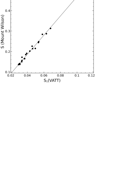
Figure 1.— The $S_{1}\rightarrow S_{\rm MW}$ (Mount Wilson) transformation for VATTspec spectra. The calibration is linear, and has no significant color term.

As mentioned above the $S_{2}\rightarrow S_{\rm MW}$ and the $S_{4}\rightarrow S_{\rm MW}$ transformations are both non-linear and require a color term. The non-linear nature of these transformations is problematical when attempting an extrapolation of the transformation to very active stars. Because the resolution of the DSO spectra is $\sim 1.8$Å/2 pixels, we cannot directly measure a DSO $S_{1}$ index. However, experimentation with the VATTspec spectra suggests a solution. The actual Ca II H & K chromospheric emission in main-sequence stars is intrinsically narrow (FWHM $\sim 0.5$Å), narrower than even the 1Å passband employed by the Mount Wilson project. That flux is entirely contained in the H & K passbands employed in the $S_{1}$, $S_{2}$, and $S_{4}$ indices, but those passbands involve successively larger amounts of photospheric flux. This suggests that it should be possible to use the $S_{2}$ and the $S_{4}$ indices to extrapolate linearly to an $S_{1}$ index: $S_{1}=1.5S_{2}-0.5S_{4}$. That this is feasible can be demonstrated with the VATTspec spectra. Figure 2 shows the correlation between the directly measured VATTspec $S_{1}$ index, and $S_{1}^{\prime}$ extrapolated from $S_{2}$ and $S_{4}$. The two are linearly related, and $S_{1}^{\prime}$ can predict the directly measured $S_{1}$ index to better than $\pm$ 1%.

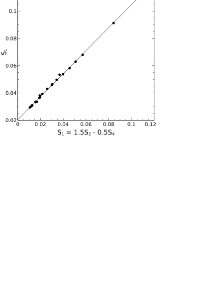
Figure 2.— The relationship between the directly measured $S_{1}$(VATT) activity index and the extrapolated $S_{1}^{\prime}$ index, based on the $S_{2}$ and $S_{4}$ indices.

This provides a way to derive a linear transformation with no color term between the instrumental DSO system and the Mount Wilson system. An $S_{1}$ extrapolated index is formed from the $S_{2}$ and $S_{4}$ instrumental indices, and that $S_{1}$ index is calibrated to the Mount Wilson $S_{\rm MW}$ index via observations of the chromospheric activity calibration stars of Gray et al. (2003). For most of those calibration stars we have only a few ($<5$) observations scattered over the past 15 years. These we refer to as “snapshot” observations. However, as part of the YSA project we have intensively observed eight Mount Wilson stars – HD 45067, HD 143761, HD 207978, HD 82885, HD 101501, HD 152391, HD 154417, and HD 206860. The first three of these stars are regularly observed “chromospherically stable stars” used to monitor the stability of our instrumental system (see below), and the latter five are active G-type stars. For these stars, we can form multi-year means for the instrumental indices that are much better correlated with the Mount Wilson means than the snapshot observations of the other calibration stars. In deriving the calibration, we give the snapshot observations a weight of 1 and the multi-year means a weight of 5. This yields the calibration (see Figure 3):

$$S_{\rm MW}=0.0323+4.8335S_{1}\quad\sigma=0.0077$$

The residuals from the calibration show no evidence for a color term. In addition, as the figure illustrates, extrapolation of this linear relationship seems to hold for very active stars.

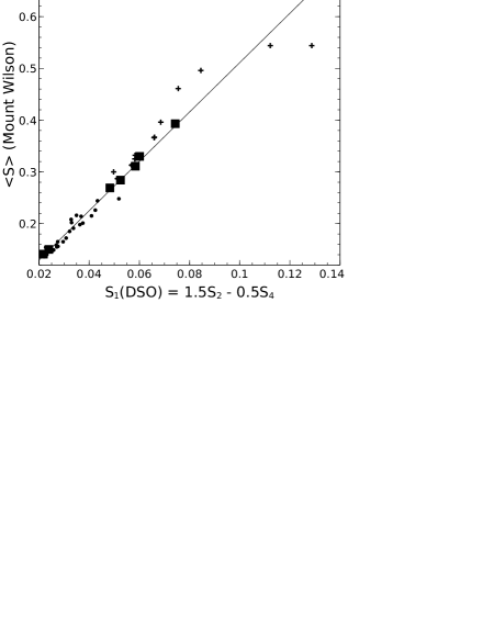
Figure 3.— The DSO $S_{1}\rightarrow S_{\rm MW}$(Mount Wilson) calibration. The ordinate is the mean Mount Wilson $\langle S_{\rm MW}\rangle$ index (Baliunas et al., 1995). The small circles represent snapshot (single to a few) observations of the Mount Wilson calibration stars (Gray et al., 2003). The large squares represent Mount Wilson stars that have been regularly observed at DSO since 2007. For these stars the 8-year mean $S_{1}$ index (in some cases derived from over a hundred observations) is used. These stars are given five times the weight of the snapshot stars in deriving the calibration. Finally, the crosses represent individual snapshot observations of very active Mount Wilson stars. These stars were not used in the derivation of the calibration, but indicate that extrapolation of the calibration is adequate even for very active stars.

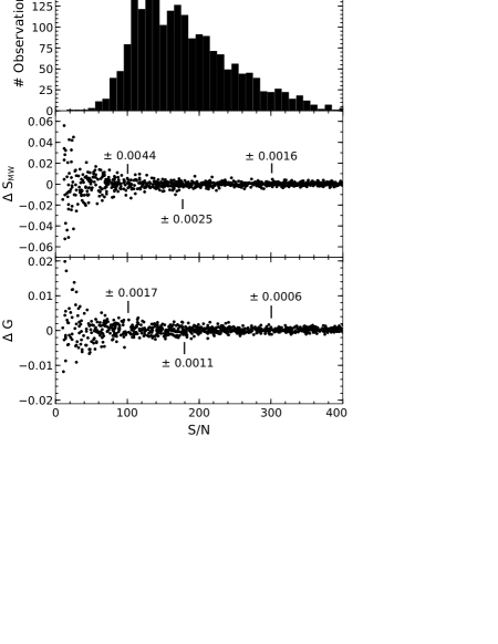
Figure 4.— The top panel shows the histogram of the S/N values of our observations. The S/N values are estimated in the continuum just longwards of the Ca II H line. The arrow indicates the average S/N, about 180. The central panel shows the results of a Monte Carlo simulation of the measurement error of $S_{\rm MW}$ as a function of S/N. At S/N = 180, the measurement error is about $\pm 0.0025$. The bottom panel shows a similar simulation for the G-band index. While the S/N in the continuum at the G-band is $\sim 1.3$ – $1.4$ times that just longwards of the Ca II H line, we have plotted, for simplicity, the G-band errors against the H-line S/N. At S/N = 180, the measurement error in the G-band index is approximately $\pm 0.0005$.

The precision of our determinations of $S_{\rm MW}$ depend on the S/N of the observations. We have attempted to estimate those precisions via a Monte-Carlo method that begins with a synthetic spectrum of the Ca II H & K region smoothed to a resolution of 1.8Å/2 pixels (the resolution of the DSO spectra). The Monte-Carlo technique simulates exposing on the spectrum until a certain S/N is achieved in the continuum just longwards of Ca II H. That exposure is processed through our measuring programs in exactly the same way as the real spectra, including the velocity correction (the synthetic spectra are given random radial velocity shifts between $-30$ and $+30$ km/s), measurements of $S_{2}$, $S_{4}$, the calculation of $S_{1}$, and the transformation to the Mount Wilson system) enabling a calculation of the error $\Delta S_{\rm MW}$ for a given simulation. Those errors are plotted against S/N in the middle panel of Figure 4. In the top panel of that same Figure is a histogram of the S/N values of our observations. The average S/N $\sim 180$, for which a measurement precision of $\pm 0.003$ in the $S_{\rm MW}$ index is estimated. Indeed this error estimate (which does not include any possible systematic errors in the transformation of our instrumental system to the Mount Wilson system) is consistent with our measurements of $S_{1}$ in the set of “chromospherically stable” stars (see below). The bottom panel of the figure shows a similar calculation for the G-band index (see below).

4.1.3 Stability of the Dark Sky Observatory Instrumental System

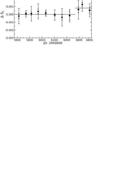
Figure 5.— The seasonal mean residuals in the instrumental $S_{1}$ index observed for the three chromospherically “stable” stars, HD 45067 (filled circles), HD 143761 (diamonds), HD 207978 (squares). The outer “error” bars indicate the standard deviation in the measured index for a given season. The inner error bars indicate the standard error of the mean. This diagram and similar ones for the other instrumental indices for the G-band, Ca I, and H$\gamma$ can be used to assess the stability of the instrumental system and to derive corrections to apply to the observed indices.

To monitor the stability of the Dark Sky Observatory instrumental system, we have regularly observed for the past 5 years, every clear night, at least one chromospherically “stable” star, chosen from a set of stars showing flat activity on the Mt. Wilson project (Baliunas et al., 1995). The stable stars that we observe are HD 45067, HD 143761, and HD 207978. During the course of an observing season, the standard deviations for night-to-night variations of those stars range from 0.0004 – 0.0012 in $S_{1}$. The lower figure in that range translates to a standard deviation in $S_{\rm MW}\sim 0.0019$, in line with our Monte Carlo estimates for the observational error in that index. To monitor any changes in the instrumental system, we have adopted the period July 1, 2011 (MJD = JD - 2450000 = 5743) to June 30, 2013 (MJD = 6445) as the reference zeropoint baseline for the instrumental system. Residuals in the seasonal means of the instrumental indices relative to that baseline will then reveal changes in the instrumental system. This is illustrated in Figure 5 for the $S_{1}$ index.

That figure shows that the instrumental system has remained very stable from the time that we began regular monitoring of the chromospherically stable stars. However, beginning September 1, 2013 (MJD = JD - 2450000 = 6536), there was a very small but abrupt shift in the instrumental system. That shift can be traced to the return of the CCD to the manufacturers for repairs because of the failure of the vacuum seal. During that visit, not only was the vacuum seal repaired, but a new driver was installed that fixed a very low-level but variable bias pattern. In addition, improved optical baffling was installed in the interior of the CCD housing which may have slightly reduced the already very low level of scattered light. To correct for this shift in the instrumental system, we subtract 0.0007 from the $S_{1}$ indices obtained since September 1, 2013. That correction may be propagated, if required, to the $S_{2}$ and $S_{4}$ indices using the relationships between those indices. We have derived similar very small corrections to the other observed indices.

Before April 2009, the spectroscopic data for this project were obtained with a Tektronics CCD (see §2.1) on the same spectrograph. We have investigated the difference in the instrumental system between the two CCDs using spectra of inactive F-, G- and K-type stars taken with both CCDs and find a small systematic difference between the two systems of 0.0019 in the measurement of the $S_{1}$ index. This correction has been applied to the earlier data.

4.2. The G-band Index

Table 3Band definitions for the Photospheric Indices

Band Name	Violet Edge	Red Edge
Continuum ($c_{1}$)	4208.0Å	4214.0Å
Ca I 4226.7Å	4225.7Å	4227.7Å
Continuum ($c_{2}$)	4239.4Å	4245.4Å
Continuum ($c_{3}$)	4263.0Å	4266.0Å
G-band	4298.0Å	4312.0Å
Continuum ($c_{4}$)	4316.0Å	4320.5Å
Continuum ($c_{5}$)	4329.0Å	4334.0Å
H$\gamma$	4339.5Å	4341.5Å
Continuum ($c_{6}$)	4345.0Å	4349.5Å

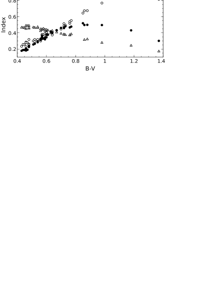
Figure 6.— The variation of the three photospheric indices defined in this paper as a function of $B-V$ color and spectral type. The G-band (solid circles) comes to a maximum in the early K-type stars, and then declines. The Ca I index (open circles) grows with increasing $B-V$ linearly until the mid K-type stars, after which it appears to saturate. The H$\gamma$ index (open triangles) decreases linearly with increasing $B-V$. The stars used for this diagram are the Mount Wilson calibration stars of Gray et al. (2003), and the $B-V$ data are from Mermilliod, Mermilliod, & Hauck (1997).

At the suggestion of Hall (2008), an index has been designed to measure the G-band molecular feature in the blue-violet region of the spectrum. This wide, deep feature arises from the blended Q-branches of the 0-0 and 1-1 vibrational bands of the diatomic CH molecule. The G-band appears first in the early F-type stars, strengthens through the F- and G-type stars, comes to a broad maximum in the early K-type stars on the main sequence, and then weakens toward later types (see Gray & Corbally, 2009). The G-band index is measured by numerically integrating the stellar monochromatic flux in a 14Å rectangular band centered at 4305Å (corresponding closely to the visible extent of the G-band in low-resolution spectra, and similar to the passband of G-band interference filters used in observations of the sun) and ratioing that with “continuum” fluxes measured in two bands on either side of the G-band (see Table 3). The G-band index is defined as:

$$1-\frac{\frac{1}{14\textrm{\AA}}\int_{4298\textrm{\AA}}^{4312\textrm{\AA}}I(\lambda)d\lambda}{0.247c_{3}+0.753c_{4}}$$

where $c_{3}$ and $c_{4}$ represent the monochromatic fluxes in the two continuum bands, respectively. Because the continuum bands are not situated symmetrically relative to the G-band passband, the weightings in the denominator are designed to give the “continuum” value at the wavelength of the center of the G-band passband. The ratio is subtracted from unity to give an index that varies between 0 and 1: 0 when the G-band is absent, 1 when the G-band is perfectly black. As expected, the G-band index is a strong function of $B-V$ (see Figure 6) and the spectral type. The G-band index will also be a function of metallicity and $\log g$ (see Gray & Corbally, 2009). We investigate in §5.2 the relationship of the G-band index to stellar activity.

A Monte Carlo error analysis similar to that described for the $S_{\rm MW}$ index was carried out for the G-band index. This is illustrated in the lower panel of Figure 4. The typical measurement error for the G-band index at S/N $=100$ is $\pm 0.0017$ and at S/N $=180$ is $\pm 0.0011$. The Monte Carlo analysis appears to have captured the important sources of measurement error for the G-band, as may be deduced from Figure 7, where the standard deviations of the seasonal G-band data for all the program stars and the “chromospherically stable” reference stars are plotted against the G-band index. The horizontal line in that figure, which corresponds well with the lower envelope of the points, is the Monte Carlo G-band error for S/N $=180$. The dispersions that lie above that line presumably arise from actual stellar variability, a point that will be considered in §5.2 below.

Figure 7.— Verification of the Monte Carlo error analysis for the G-band index. This figure plots the seasonal dispersions ($\sigma$) of the G-band indices for all of the program stars plus the chromospherically stable reference stars against the G-band index. The horizontal line, which corresponds well with the lower envelope of the distribution of points, represents the Monte Carlo error calculation for S/N $=180$, the average S/N of our spectra.

4.3. The Ca I Index

Another prominent absorption feature in the blue-violet spectrum of G- and K-type stars is the resonance line of Ca I at 4226.7Å. This absorption line grows steadily in strength toward later types, at least up to mid K-type stars. It is also sensitive to surface gravity, especially in the K-type stars (see Gray & Corbally, 2009). We have devised an index similar to that of the previously defined G-band index. The Ca I index is measured by integrating over a 2Å-wide band centered on the Ca I line and ratioing that with fluxes in two symmetrically placed continuum bands. The formula used is:

$$1-\frac{\frac{1}{2\textrm{\AA}}\int_{4225.7\textrm{\AA}}^{4227.7\textrm{\AA}}I(\lambda)d\lambda}{0.5(c_{1}+c_{2})}$$

where $c_{1}$ and $c_{2}$ are the continuum bands defined in Table 3. As can be seen in Figure 6, the Ca I index behaves as designed; it grows linearly from the F-type stars into the K-type stars, only saturating after a spectral type of K3.

A Monte Carlo error analysis similar to that illustrated in Figure 4 was carried out for the Ca I index, giving a measurement error of $\pm 0.0027$ at S/N $=180$. This value again corresponds well with the lower envelope of Ca I index seasonal dispersions (see discussion in §4.2 above).

4.4. The H$\gamma$ Index

Both the G-band index and the Ca I index grow with decreasing temperature (at least up to the early K-type stars), and so it is useful to define another index that decreases with the temperature. The hydrogen lines behave in exactly this way in the F-, G-, and K-type stars. The best hydrogen line to use in the spectral range provided by our spectra from the Dark Sky Observatory is H$\gamma$. An index based on the H$\beta$ line would probably be preferable, because of the less crowded surroundings, but that line is outside our spectral range. The H$\gamma$ index is defined similarly to the Ca I index, with a 2Å-wide band centered on the H$\gamma$ line and flanking “continuum” bands (specified in Table 3). The formula used is

$$1-\frac{\frac{1}{2\textrm{\AA}}\int_{4339.5\textrm{\AA}}^{4341.5\textrm{\AA}}I(\lambda)d\lambda}{0.4286c_{5}+0.5714c_{6}}$$

The H$\gamma$ index behaves as designed, declining in strength with declining temperature (Figure 6). However, it appears to have only about half the temperature sensitivity of the Ca I index.

A Monte Carlo error analysis similar to that illustrated in Figure 4 was carried out for the H$\gamma$ index, giving a measurement error of $\pm 0.0020$ at S/N $=180$. The larger errors for the Ca I and H$\gamma$ indices relative to the G-band index arise primarily from the narrower “science” bands.

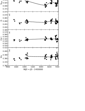
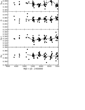
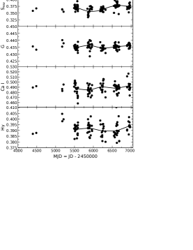
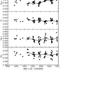
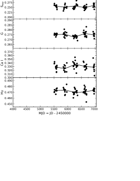
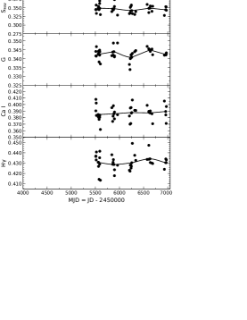
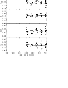
Figure 8.— A montage of Ca II H & K activity index ($S_{\rm MW}$) time series (upper panel), and G-band index, Ca I, and H$\gamma$ times series (lower panels) for our program stars (montage continued in Figures 9, 10, and 11). All the graphs are scaled identically, with a range of 0.15 in $S_{\rm MW}$, 0.03 in the G-band index, 0.08 in the Ca I index, and 0.05 in the H$\gamma$ index so that amplitudes of variations and seasonal dispersions can be intercompared directly. The solid lines are Bezier curves drawn through the seasonal means. Typical error bars for S/N $=180$ spectra are shown in the upper left-hand corner of the panels for the first star.

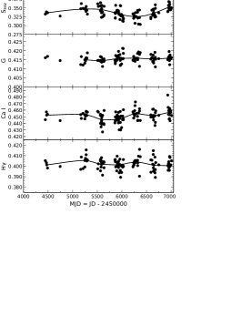
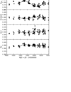
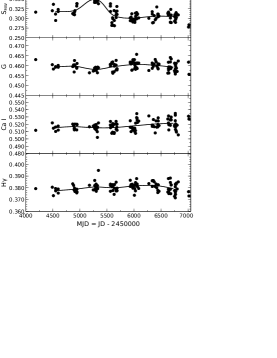
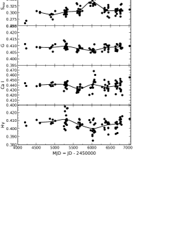
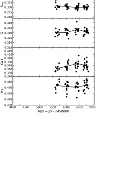
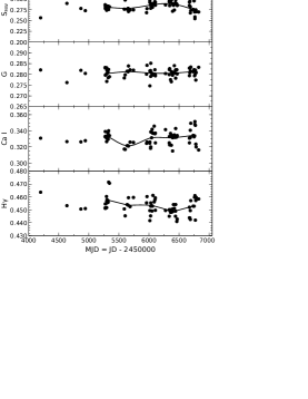
Figure 9.— Continuation of the montage in Figure 8.

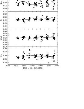
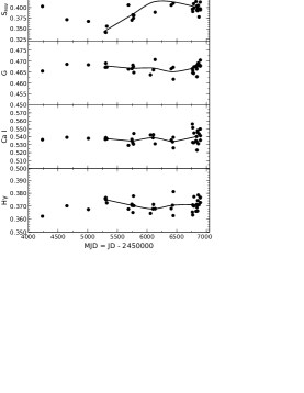
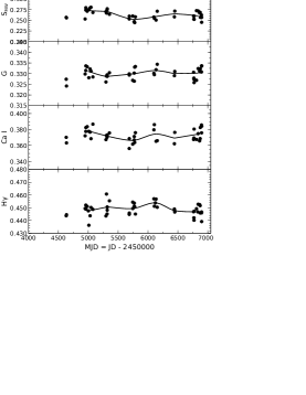
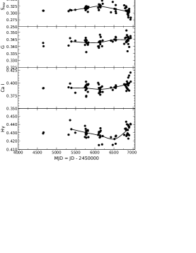
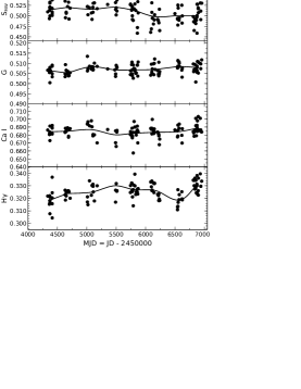
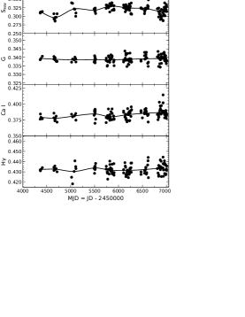
Figure 10.— Continuation of the montage in Figures 8 and 9.

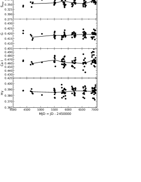
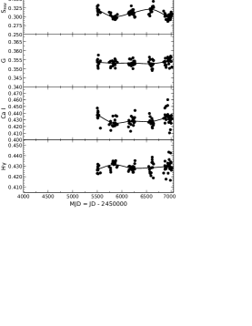
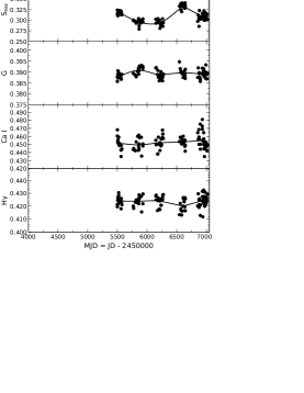
Figure 11.— Continuation of the montage in Figures 8, 9, and 10.

5. Statistical Analysis of the Spectroscopic Results

Table 4Young Solar Analog Stars
Mean Activity Data, Predicted Rotational Periods in days, and Chromospheric Activity Ages

Name	$\langle S_{\rm MW}\rangle$	$\sigma$	$\langle\log(R^{\prime}_{\rm HK})\rangle$	$P_{\rm rot}(R^{\prime}_{\rm HK})$	$P_{\rm max}(v\sin i)$	Age	$\langle$G$\rangle$	$\sigma$	$\langle$Ca I$\rangle$	$\sigma$	$\langle$H$\gamma\rangle$	$\sigma$
				00(error)	00(error)	(Myr)
HD 166	0.429	0.017	-4.393	7.52d (2.79)	10.03d (0.45)	375	0.459	0.002	0.539	0.006	0.384	0.005
HD 5996	0.376	0.019	-4.465	11.30d (2.80)	0000$\infty$	763	0.463	0.002	0.528	0.009	0.366	0.005
HD 9472	0.322	0.011	-4.495	10.06d (2.19)	16.23d (1.05)	762	0.408	0.002	0.448	0.009	0.405	0.005
HD 13531	0.369	0.013	-4.431	8.06d (2.37)	7.38d (0.12)	486	0.436	0.002	0.488	0.009	0.391	0.005
HD 27685	0.310	0.017	-4.510	10.14d (2.08)	32.71d (20.45)	810	0.425	0.002	0.456	0.010	0.410	0.006
HD 27808	0.255	0.011	-4.541	4.36d (0.80)	5.15d (0.08)	548	0.275	0.002	0.330	0.010	0.472	0.004
HD 27836	0.346	0.011	-4.397	4.03d (1.46)	000 $\cdots$	210	0.343	0.003	0.387	0.011	0.431	0.008
HD 27859	0.312	0.009	-4.460	5.80d (1.47)	8.14d (0.22)	390	0.360	0.002	0.391	0.011	0.436	0.005
HD 28394	0.259	0.007	-4.520	3.46d (0.69)	3.01d (0.14)	876	0.241	0.002	0.307	0.011	0.479	0.006
HD 42807	0.339	0.013	-4.451	7.58d (2.01)	8.91d (0.36)	494	0.416	0.002	0.450	0.008	0.402	0.005
HD 76218	0.392	0.019	-4.458	11.37d (2.91)	12.54d (0.74)	753	0.470	0.003	0.570	0.010	0.362	0.006
HD 82885	0.287	0.018	-4.632	20.77d (2.91)	16.00d (1.00)	2184	0.479	0.002	0.551	0.007	0.389	0.003
HD 96064	0.476	0.028	-4.355	5.81d (1.82)	15.61d (2.79)	230	0.453	0.003	0.544	0.012	0.368	0.008
HD 101501	0.315	0.019	-4.540	13.90d (2.56)	15.55d (2.22)	1185	0.460	0.002	0.518	0.007	0.380	0.004
HD 113319	0.303	0.020	-4.511	9.37d (1.92)	12.77d (0.71)	743	0.408	0.002	0.439	0.008	0.406	0.007
HD 117378	0.302	0.010	-4.452	4.20d (1.11)	4.73d (0.09)	297	0.331	0.003	0.368	0.011	0.433	0.007
HD 124694	0.282	0.010	-4.473	3.35d (0.80)	3.08d (0.09)	344	0.281	0.002	0.331	0.008	0.453	0.006
HD 130322	0.253	0.030	-4.720	26.31d (3.01)	0000$\infty$	3202	0.484	0.004	0.564	0.011	0.363	0.004
HD 131511	0.445	0.021	-4.455	12.57d (3.27)	9.49d (0.40)	797	0.496	0.002	0.611	0.006	0.357	0.005
HD 138763	0.316	0.012	-4.436	4.46d (1.28)	000 $\cdots$	283	0.322	0.002	0.366	0.009	0.440	0.008
HD 149661	0.303	0.019	-4.651	24.23d (3.24)	27.73d (3.70)	2581	0.506	0.002	0.623	0.007	0.352	0.004
HD 152391	0.391	0.022	-4.445	10.28d (2.81)	10.35d (0.48)	651	0.467	0.002	0.538	0.007	0.371	0.005
HD 154417	0.263	0.010	-4.550	6.92d (1.23)	8.12d (0.24)	654	0.330	0.002	0.373	0.007	0.448	0.005
HD 170778	0.315	0.014	-4.444	4.97d (1.37)	6.35d (0.16)	322	0.344	0.003	0.392	0.008	0.430	0.007
HD 189733	0.510	0.021	-4.503	16.91d (3.57)	13.58d (0.94)	1167	0.507	0.002	0.685	0.007	0.325	0.007
HD 190771	0.326	0.011	-4.462	7.37d (1.85)	9.61d (0.36)	492	0.401	0.002	0.453	0.007	0.421	0.005
HD 206860	0.317	0.014	-4.438	4.73d (1.34)	5.01d (0.05)	305	0.339	0.002	0.384	0.007	0.433	0.004
HD 209393	0.360	0.013	-4.429	7.38d (2.19)	10.61d (0.53)	440	0.419	0.002	0.464	0.010	0.387	0.005
HD 217813	0.310	0.012	-4.462	5.82d (1.47)	11.89d (0.54)	397	0.353	0.002	0.430	0.008	0.429	0.004
HD 222143	0.310	0.015	-4.497	8.87d (1.92)	16.55d (1.03)	675	0.389	0.002	0.452	0.008	0.424	0.005

Table 5Index-Variation Kolmogorov-Smirnov Significance Tests
Probability of the Null Hypothesis

Star ID	$S_{\rm MW}$	G-band	Ca I	H$\gamma$	$N_{\rm seasons}$
HD 166	$<10^{-5}$	0.020	$\cdots$	$\cdots$	4
HD 5996	$<10^{-5}$	0.028	0.0023	$\cdots$	5
HD 9472	0.00075	$<10^{-5}$	$\cdots$	$\cdots$	5
HD 13531	$<10^{-5}$	0.030	$\cdots$	0.024	5
HD 27685	$<10^{-5}$	0.00002	$\cdots$	$\cdots$	6
HD 27808	$\cdots$	$<10^{-5}$	$\cdots$	$\cdots$	5
HD 27836	$\cdots$	$\cdots$	$\cdots$	$\cdots$	5
HD 27859	0.011	$\cdots$	$\cdots$	$\cdots$	5
HD 28394	0.014	$\cdots$	$\cdots$	$\cdots$	5
HD 42807	$<10^{-5}$	0.014	$<10^{-5}$	0.0153	6
HD 76218	$<10^{-5}$	$\cdots$	0.00033	$\cdots$	7
HD 82885	$<10^{-5}$	0.00059	0.0011	0.00026	7
HD 96064	$<10^{-5}$	0.029	0.00019	$\cdots$	8
HD 101501	$<10^{-5}$	0.00033	0.0045	0.013	7
HD 113319	$<10^{-5}$	0.00046	0.0014	0.00045	6
HD 117378	$\cdots$	$\cdots$	$\cdots$	$\cdots$	4
HD 124694	$<10^{-5}$	$\cdots$	0.00069	0.00016	5
HD 130322	$<10^{-5}$	$\cdots$	0.033	$\cdots$	5
HD 131511	0.025	$\cdots$	$\cdots$	0.038	7
HD 138763	0.00076	$\cdots$	$\cdots$	0.023	6
HD 149661	0.00043	$\cdots$	$\cdots$	$\cdots$	4
HD 152391	$\cdots$	$\cdots$	$\cdots$	$\cdots$	4
HD 154417	0.00075	$\cdots$	$\cdots$	$\cdots$	5
HD 170778	0.00022	$\cdots$	$\cdots$	0.0011	5
HD 189733	0.00097	0.015	$\cdots$	$<10^{-5}$	8
HD 190771	0.0005	0.024	0.049	0.010	6
HD 206860	$<10^{-5}$	$\cdots$	0.0031	$\cdots$	6
HD 209393	0.00036	0.048	$\cdots$	$\cdots$	5
HD 217813	$<10^{-5}$	$\cdots$	$<10^{-5}$	$\cdots$	5
HD 222143	$<10^{-5}$	0.0011	$\cdots$	$\cdots$	5

Table 6Pearson Statistical Tests of Index-to-Index Correlations

Star ID	$S_{\rm MW}-G$	$S_{\rm MW}-Ca~{}I$	$S_{\rm MW}-H\gamma$	$G-Ca~{}I$	$G-H\gamma$	$Ca~{}I-H\gamma$
HD 166	$+0.216,0.117$	$-0.137,0.323$	$-0.091,0.511$	$-0.066,0.634$	$+0.039,0.779$	$-0.234,0.089$
HD 5996	$-0.190,0.081$	$-0.102,0.351$	$-0.236,0.030$	$\mathbf{+0.479,0.000}$	$\mathbf{+0.379,0.000}$	$+0.226,0.038$
HD 9472	$-0.025,0.843$	$-0.170,0.175$	$-0.066,0.603$	$\mathbf{+0.330,0.007}$	$+0.214,0.086$	$+0.222,0.075$
HD 13531	$-0.106,0.338$	$+0.055,0.621$	$-0.093,0.400$	$+0.257,0.018$	$\mathbf{+0.489,0.000}$	$+0.178,0.106$
HD 27685	$\mathbf{-0.391,0.001}$	$+0.267,0.033$	$-0.205,0.104$	$+0.133,0.295$	$\mathbf{+0.330,0.008}$	$\mathbf{+0.360,0.004}$
HD 27808	$-0.215,0.102$	$-0.146,0.268$	$-0.188,0.153$	$+0.021,0.875$	$+0.091,0.494$	$-0.104,0.435$
HD 27836	$+0.050,0.767$	$-0.024,0.887$	$-0.111,0.514$	$+0.363,0.027$	$\mathbf{+0.558,0.000}$	$\mathbf{+0.499,0.002}$
HD 27859	$+0.074,0.682$	$+0.044,0.809$	$-0.083,0.647$	$+0.062,0.731$	$+0.158,0.381$	$+0.258,0.147$
HD 28394	$-0.185,0.240$	$-0.208,0.186$	$\mathbf{-0.506,0.001}$	$-0.057,0.722$	$+0.363,0.018$	$+0.221,0.160$
HD 42807	$\mathbf{-0.291,0.004}$	$+0.044,0.675$	$-0.245,0.017$	$+0.151,0.144$	$\mathbf{+0.390,0.000}$	$+0.208,0.043$
HD 76218	$\mathbf{-0.323,0.000}$	$+0.019,0.837$	$-0.170,0.066$	$\mathbf{+0.496,0.000}$	$\mathbf{+0.579,0.000}$	$\mathbf{+0.570,0.000}$
HD 82885	$\mathbf{-0.464,0.000}$	$\mathbf{-0.292,0.002}$	$+0.113,0.241$	$+0.155,0.108$	$\mathbf{+0.249,0.009}$	$+0.064,0.507$
HD 96064	$-0.164,0.142$	$-0.030,0.787$	$\mathbf{-0.296,0.007}$	$\mathbf{+0.425,0.000}$	$\mathbf{+0.404,0.000}$	$\mathbf{+0.279,0.011}$
HD 101501	$\mathbf{-0.351,0.000}$	$-0.135,0.168$	$-0.021,0.830$	$-0.017,0.866$	$\mathbf{+0.388,0.000}$	$-0.016,0.869$
HD 113319	$\mathbf{-0.508,0.000}$	$-0.038,0.731$	$\mathbf{-0.493,0.000}$	$+0.053,0.627$	$\mathbf{+0.503,0.000}$	$+0.135,0.212$
HD 117378	$+0.045,0.756$	$-0.187,0.193$	$\mathbf{-0.501,0.000}$	$-0.073,0.615$	$-0.075,0.606$	$\mathbf{+0.345,0.014}$
HD 124694	$-0.266,0.032$	$-0.053,0.677$	$\mathbf{-0.457,0.000}$	$+0.133,0.292$	$+0.103,0.413$	$+0.190,0.129$
HD 130322	$\mathbf{-0.429,0.003}$	$+0.046,0.762$	$-0.010,0.943$	$\mathbf{+0.390,0.007}$	$+0.258,0.082$	$\mathbf{+0.481,0.001}$
HD 131511	$\mathbf{-0.307,0.010}$	$-0.165,0.176$	$-0.115,0.347$	$+0.166,0.172$	$\mathbf{+0.320,0.007}$	$+0.181,0.138$
HD 138763	$+0.055,0.730$	$-0.253,0.106$	$-0.350,0.023$	$\mathbf{+0.500,0.001}$	$\mathbf{+0.490,0.001}$	$\mathbf{+0.520,0.000}$
HD 149661	$\mathbf{-0.442,0.005}$	$\mathbf{-}0.346,0.031$	$+0.102,0.536$	$+0.364,0.023$	$+0.317,0.049$	$-0.130,0.430$
HD 152391	$-0.414,0.026$	$-0.068,0.726$	$-0.281,0.140$	$+0.194,0.314$	$+0.129,0.505$	$-0.085,0.662$
HD 154417	$-0.090,0.635$	$-0.041,0.831$	$+0.072,0.706$	$+0.187,0.323$	$-0.005,0.980$	$-0.106,0.578$
HD 170778	$-0.152,0.277$	$\mathbf{-0.524,0.000}$	$\mathbf{-0.385,0.004}$	$+0.223,0.108$	$+0.301,0.029$	$\mathbf{+0.361,0.008}$
HD 189733	$-0.116,0.245$	$-0.067,0.502$	$-0.017,0.867$	$\mathbf{+0.341,0.000}$	$+0.210,0.033$	$\mathbf{+0.262,0.007}$
HD 190771	$\mathbf{-0.307,0.003}$	$\mathbf{-0.285,0.006}$	$-0.240,0.022$	$\mathbf{+0.289,0.006}$	$+0.177,0.095$	$\mathbf{+0.266,0.011}$
HD 206860	$-0.073,0.466$	$\mathbf{-0.470,0.000}$	$\mathbf{-0.445,0.000}$	$+0.164,0.102$	$+0.066,0.513$	$+0.177,0.076$
HD 209393	$\mathbf{-0.270,0.011}$	$+0.078,0.466$	$-0.208,0.051$	$\mathbf{+0.473,0.000}$	$+0.220,0.038$	$+0.189,0.077$
HD 217813	$-0.228,0.038$	$-0.192,0.081$	$\mathbf{-0.284,0.009}$	$+0.200,0.070$	$+0.191,0.083$	$-0.049,0.662$
HD 222143	$-0.089,0.411$	$-0.006,0.959$	$-0.211,0.050$	$-0.053,0.623$	$+0.163,0.131$	$+0.097,0.372$

Figures 8, 9, 10, and 11 show montages (in order of HD number) of time series of the Ca II H & K index (transformed to the Mount Wilson system index $S_{\rm MW}$), the G-band index, the Ca I index, and the H$\gamma$ index for our program stars.

Table 4 lists mean values for the $S_{\rm MW}$ index and $\log(R^{\prime}_{\rm HK})$ from our observations of the program stars. The $S_{\rm MW}$ index measures the flux in the cores of the Ca II H & K lines, but that flux includes contributions from both the chromosphere and the photosphere. A quantity $R^{\prime}_{\rm HK}$, which is a useful measure of the chromospheric flux only, may be derived from $S_{\rm MW}$ using a method outlined in Noyes et al. (1984). The $\log(R^{\prime}_{\rm HK})$ index may be calibrated against age and rotation period (Mamajek & Hillenbrand, 2008). We have included columns in Table 4 listing the expected rotation period (in days), $P_{\rm rot}(R^{\prime}_{\rm HK})$, based on the calibration of Mamajek & Hillenbrand (2008), as well as the upper limit to the rotation period derived from our $v\sin i$ values listed in Table 2 ($P_{\rm max}(v\sin i)$), along with associated errors. Note that, with the possible exception of HD 82885, the rotation periods derived from the activity levels are consistent, within the errors, with the rotation period upper limits deduced from the projected rotational velocities. Chromospheric “activity ages” for our program stars, based on the calibration of Mamajek & Hillenbrand (2008), are also included in Table 4. As it turns out, all but three of our stars (HD 82885, HD 130322, and HD 149661) lie within the target age limits for this project, 0.3 – 1.5 Gyr. However, the discrepancy between $P_{\rm rot}(R^{\prime}_{\rm HK})$ and $P_{\rm max}(v\sin i)$ for HD 82885 suggests that the chromospheric activity age for that star may not be accurate. For instance, Donahue, Saar, & Baliunas (1996) quote a rotation period for HD 82885 of 18.6 days. This gives a gyrochronological age, using the calibration of Barnes (2007), of 1.6 Gyr.

5.1. The Sensitivity of the Photospheric Indices to Temperature Variations

It was hypothesized in the Introduction that the three “photospheric” indices defined in §4.2 – 4.4 will be primarily sensitive to temperature, and thus might be useful in measuring integrated temperature changes on the stellar surface arising from spots and/or photospheric faculae. To determine the usefulness of these indices for that purpose, we need to assess their sensitivity to these changes. Figure 6 displays plots of these indices (using the Mount Wilson calibration stars from Table 5 of Gray et al. (2003)) versus $B-V$. That Figure shows that in the realm of the late F-type stars to the early K-type stars all three indices vary approximately linearly with $B-V$. The following equations are straight-line fits to the linear portions of those curves:

$$B-V=\, 0.259+0.966\,{\rm G}$$

$$B-V=\, 0.212+1.010\,{\rm Ca\,I}$$

$$B-V=\, 1.68-2.539\,{\rm H}\gamma$$

where G, Ca I, and H$\gamma$ refer to their respective indices, and $B-V$ refers to the Johnson $B-V$ index. Both the G-band index and the Ca I index have slopes of nearly unity with respect to $B-V$, and so changes in those indices should translate directly into changes in $B-V$. The H$\gamma$ index has a sensitivity that is smaller by about a factor of 2.5.

We will report in Paper II that many of our stars vary $\leq 0.03$ – 0.07 magnitude in the Johnson $V$-band, and in the instances where we can measure color ($B-V$) changes, those changes are generally $\leq 0.01$ mag. This is roughly what we might expect if variations in brightness (due to sunspots and faculae) move the star parallel to the main sequence. If the observed changes in the photospheric indices arise solely from temperature effects, we might therefore expect to observe variations in the G-band and Ca I up to 0.01 in the index, and by a factor of about 2.5 smaller in H$\gamma$. Such changes should be detectable in at least the G-band and Ca I indices, as the measurement errors in those indices are on the order of 0.001 – 0.003. Indeed, because of those measurement errors, these indices are potentially more useful in measuring temperature changes than photometric colors where the errors are larger. Interestingly, the data in Table 4 do indeed indicate variations in Ca I of about the expected magnitude ($\leq 0.01$), but the observed variations in the G-band are smaller by a factor of two or more ($\leq 0.004$). Hence, while it is plausible that the observed variations in Ca I are temperature related, it is clear that the variations in the G-band may have a different or more complex origin. The observed variations in H$\gamma$ are smaller than those observed in Ca I, but not by the factor we would expect if those variations are governed by temperature alone. We will examine these questions in more detail in §5.4 below.

5.2. Statistical Tests for Season-to-Season Variability

The $S_{\rm MW}$ plots are the traditional tool for detecting and characterizing activity cycles in stars. The detection and characterization of activity cycles in active stars requires time series observations that exceed, preferably by a factor of two or more, the period or characteristic timescale of the star in question. That normally requires observations over decades, and so, except for stars that our program has in common with other long-term surveys, such as the Mt. Wilson program, we are limited in what we can say on that subject. What can be done at the current stage of the project is to 1) evaluate the reality of the variations in the seasonal means and/or variances of the four “activity” indices – the $S_{\rm MW}$, G-band, Ca I, and H$\gamma$ indices – that are suggested by the time series montages and 2) to examine and try to understand the existence of correlations between those indices.

To assess the significance of the variations in the four indices on a year-to-year basis (variations within a given observing season will be examined in Paper II of this series where we will evaluate rotation periods for our stars), we have employed the Kolmogorov-Smirnov (KS) statistical test. KS tests are used in judging the significance of whether or not two experimental or observational distributions of a certain variable differ; the difference may arise from either a difference in the means or in the variances of the two distributions. We may consider each set of seasonal data (the “clumps” in Figures 8, 9, 10, and 11) as independent samples of the index in question, and compare those samples for a given star on a pair-wise basis using the KS test to ascertain whether significant variation in the mean value and/or variance of the index has occured over the period we have observed the star. The way we perform the tests is as follows. Let us suppose we have observed the star for four years (four observing seasons), seasons 1, 2, 3, and 4. We then carry out KS tests on each of the following six pair-wise comparisons: $1\leftrightarrow 2$, $1\leftrightarrow 3$, $1\leftrightarrow 4$, $2\leftrightarrow 3$, $2\leftrightarrow 4$, and $3\leftrightarrow 4$. The KS test yields a $p$-statistic for each comparison. Smaller values of $p$ indicate higher significance. For instance, $p=0.01$ indicates that the null hypothesis (no variation in the mean value or variance of the index) may be rejected with a confidence of 99%. But the fact that we need to estimate the significance of variations in a time series rather than simply between two seasons complicates the analysis. For instance, let us suppose we have five seasons of observations. This results in a set of 10 pair-wise comparisons. If only one of those comparisons results in $p=0.01$, that does not rise to the level of significance because we would expect, on the average, in a set of 10 comparisons, to encounter $p\leq 0.01$ 10% of the time – a significance of only 90%. However, if a given set contains multiple comparisons with small $p$, we may then combine those probabilities in assessing the significance of the observed variation.

We use a Monte Carlo technique to evaluate these probabilities. A random number generator was used to generate multiple gaussian distributions of an observational variable, all with the same mean and variance (and thus for these artificial data the null hypothesis is true). In total we generated 100,000 sets of 4-season data, each involving 6 pair-wise comparisons, for a total of 600,000 comparisons, and evaluated each comparison with KS statistics. We did the same for sets of 5-season, 6-, 7-, and 8-season data, the latter involving 2.8 million pair-wise comparisons. We were able to verify, for instance, that comparisons with $p\leq 0.01$ were encountered with the expected frequency. We then used these artificial data sets to evaluate the significance of variations in our observational data. To take a real example, in one of our 5-season data sets (HD 9472), we had, for the $S_{\rm MW}$ index, the following values of $p$: 0.0116, 0.0132, 0.0188, 0.0281, and 0.0315. The remaining five comparisons had $p>0.05$. We then used the 5-season Monte Carlo data to ask “What proportion of 5-season sets have $p_{\rm min}\leq 0.0116$ and four other comparisons with $p\leq 0.0315$?” The result yields an overall $p=0.00075$. We have listed in Table 5 all the time series for which the overall $p\leq 0.05$, indicating “significant” variability.

Spurious significant $p$ values can be created by outliers in the dataset. We have reduced to a minimum the number of outliers in the dataset by rejecting all spectra with S/N $<50$ and by examining each spectrum to eliminate those with obvious defects (such as cosmic rays) in the wavelength bands used for the calculation of the indices. The remaining outliers cannot be rejected on a statistical basis (and may indeed represent true excursions of the star) and so are included in the statistical tests.

It is clear from Table 5 that almost all of the program stars show significant season-to-season variations in $S_{\rm MW}$. The ones that do not have only 4 or 5 seasons of data, so it is entirely possible that with a few more seasons of data all will show significant variation. 50% show significant variations in the G-band index, 40% in the Ca I index, and 37% in the H$\gamma$ index. We expect that continuing the project for a few more years will increase those proportions as well. We emphasize that a lack of significant variation in the seasonal means and variances does not imply that the star is constant within a given season. For instance, it is well known, and we will further demonstrate in Paper II, that the “scatter” (at least for the $S_{\rm MW}$ index) within a given season can arise from rotational modulation in the index.

5.3. Comments on the Nature of the Observed Variability

A number of our stars that have significant season-to-season variations appear to be showing very short-term periodic or “pseudo periodic” behavior in the $S_{\rm MW}$ index. Examples include HD 9472, HD 13531, HD 27685 (superimposed on a secular rise in activity), HD 217813, as well as some others. Despite the shortness of the datasets, the above-mentioned stars show significant periods in the range of 2 – 4 years with a Lomb-Scargle analysis. To judge the reality of such short periods, which are considerably shorter than the periods found in Baliunas et al. (1995) we may refer to other similar datasets. For example, a number of stars in the Lockwood et al. (2007) dataset appear to show very similar behavior (see the stars HD 39587, HD 131156, HD 152391, HD 115404, HD 201092 for some possible examples). This short-term variation appears to come and go and is often superimposed on longer timescale variations. Analysis of the Lockwood et al. or similar datasets will be required to evaluate the reality of these variations.

Stars in our dataset show a variety of behaviors associated with the dispersion in the $S_{\rm MW}$ activity index within a given season. For instance, the stars HD 27859 ($\langle\sigma_{S_{\rm MW}}\rangle=0.007$), HD 124694 (0.008), HD 154417 (0.007), HD 217813 (0.008), and HD 222143 (0.006) all show very tight activity dispersions within a given season. On the other hand, HD 130322 (0.014), HD 131511 (0.018), and HD 189733 (0.018) show average seasonal dispersions greater by a factor of two or more within a given season. This distinction appears to be intrinsic, as we are careful to achieve adequate S/N for all of our observations, and there are bright and “faint” stars in both sets. We note, however, that those stars that have particularly low seasonal dispersions are F and early G-type stars, while the three with the higher dispersions are all K-type stars. If the seasonal dispersions arise from rotational modulation, as active regions rotate across the stellar disk, then this suggests that the late-type stars mentioned above may be dominated by one or a small number of active regions, whereas for the F- and early G-type stars in the project sample, active regions are smaller and more dispersed across the stellar disk. One caution should be noted: the activity behavior of HD 189733 may not be typical of young active K-type stars, as it has apparently been spun up by angular momentum transfer from its hot-jupiter companion (see Introduction). HD 131511 does, however, behave in quite a similar way to HD 189733. Even though HD 131511 is a spectroscopic binary, its stellar companion is in a much wider orbit ($P_{\rm orb}=125.4$d Nidever et al., 2002; Jancart et al., 2005), and probably has not yet had an important influence on the angular momentum of the primary. We also note that in a recent Nordic Optical Telescope FIES spectrum of HD 131511, the emission in the cores of the Ca II H & K lines appear symmetrical, and so we see no evidence for emission from the companion. This will need to be verified by further spectra at different phases of the companion’s orbit.

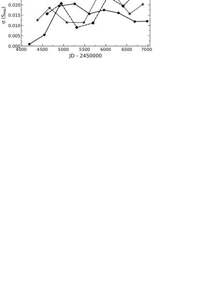
Figure 12.— The variation in the seasonal dispersion of $S_{\rm MW}$ with time for three stars, HD 76218 (solid line), HD 131511 (dashed line), and HD 189733 (dotted line).

Interestingly, some of our stars appear to show variations in their seasonal dispersion behavior. Whether that variation in dispersion is cyclical can only be determined with longer time series. The F-test is the appropriate test for determining the statistical significance of season-to-season differences in the variance of an index. HD 131511, for instance, appears to alternate between seasons with high and moderate dispersions in the $S_{\rm MW}$ index. Examination of the $S_{\rm MW}$ plot for HD 131511 (Figure 10) shows four seasons with relatively high dispersions and three with moderate dispersions. F-tests carried out on the 21 pair-wise comparisons between the seven seasons show highly significant variations, with an overall $p=0.0011$ (calculated using the same Monte Carlo technique employed to evaluate the KS tests). HD 189733 may be behaving in a similar way, although the statistics are of lower significance ($p=0.045$). HD 76218 apparently also varies in seasonal dispersion ($p=0.016$). The variation in HD 76218 is unusual in the sense that when the seasonal dispersion is the highest, the activity level is at or near a minimum. This is opposite to the sun which shows the greatest dispersion in the Ca II flux at activity maximum (Keil, Henry, & Fleck, 1998). Figure 12 shows the variation in seasonal dispersion with time for HD 76218, HD 131511, and HD 189733. A possible interpretation of this behavior is that these stars vary between a state in which the active regions are relatively small, numerous, and dispersed (low-to-moderate seasonal dispersion) and a state which is dominated by one or a few large active regions (high seasonal dispersion). This variation in seasonal dispersion may represent a novel type of activity cycle in stars, or it may be evidence for a flipflop cycle (Jetsu, Pelt & Tuominen, 1993) and/or active longitudes. More observations will be required to fully characterize this behavior.

5.4. Correlations Between Indices

A further question to address is whether or not significant correlations exist between the four “activity” indices measured in this paper. In the Introduction we gave the rational for the three “photospheric” indices defined in this paper – the G-band, Ca I, and H$\gamma$ indices – and suggested that these three indices might vary in step with activity variations largely through related temperature changes in the photosphere connected with changes in spots and photospheric faculae. How the photospheric indices would vary in relation to $S_{\rm MW}$ would then depend on whether cool spots or hot photospheric faculae dominate. If the photospheric indices vary primarily on the basis of temperature, we would expect the G-band index to vary directly with the Ca I index, and inversely with respect to the H$\gamma$ index. We will see below whether this is indeed the case.

Table 6 shows the results of Pearson’s r-tests for linear correlations between the four indices. These comparisons are made with the original observations, and not with the seasonal means. Since all of these indices are measured in a single spectrum, we do not have to worry about time differences between the observations of the different indices. The first column in Table 6 is the stellar ID, the second tabulates the results of the Pearson r-test for correlations between $S_{\rm MW}$ and the G-band index, the third the same for $S_{\rm MW}$ and Ca I, the fourth for $S_{\rm MW}$ and H$\gamma$, the fifth for the G-band and Ca I, the sixth for the G-band and H$\gamma$, and the seventh for Ca I and H$\gamma$. Each comparison consists of two numbers, Pearson’s linear correlation coefficient $r$, and the $p$-statistic, from which the probability of the null hypothesis (zero correlation) may be calculated. Small $p$ indicates a signficant correlation. Correlations with $p\leq 0.015$ are indicated with bold type in Table 6. We have adopted $p\leq 0.015$ as a useful standard for judging the significance of these correlations because, for a given index, and 30 tabulated stars, we should expect at that significance level only 0.5 spurious correlations.

A glance at Table 6 shows the presence of multiple significant, in many cases highly significant, correlations, although none of those correlations are particularly strong ($r<0.6$). We have examined each of these correlations graphically to assure ourselves that none are caused by one or a few “outliers”. Could these correlations arise from instrumental effects? We reject that for a number of reasons: 1) We have not included in these tests data from the earlier Photometrics CCD, and so that means that all of the observations involved in these tests have been carried out with the same CCD on the same spectrograph on the same telescope, and all have been reduced identically. 2) The passbands used in defining these indices do not overlap, and so a spectral defect (cosmic ray, etc.) that affects one index will not affect another. 3) While some stars show highly significant correlations, others do not. Instrumental effects would lead to significant correlations (or not) in all stars, not just a limited number.

Let us now examine the nature of those correlations. For the $S_{\rm MW}$ – G-band comparison, 11 out of the 30 stars show significant ($p\leq 0.015$) correlations, and all of those are negative correlations, meaning that in those stars $S_{\rm MW}$ and the G-band vary oppositely; when one increases, the other decreases. Note that the correlations that do not rise to our level of significance are as well almost all negative. For the $S_{\rm MW}$ – Ca I comparison, only 4 of the 30 stars show a significant correlation, but again all of those are negative. For $S_{\rm MW}$ – H$\gamma$, 8 of the 30 stars show significant correlations, and again all of those correlations are negative. So, a strong conclusion is that where significant correlations are present, the “photospheric” indices are all negatively correlated with $S_{\rm MW}$.

What about correlations between the photospheric indices? Examination of Table 6 shows the presence of many highly significant correlations between these indices, all of which are positive. So, the tendency is, when the G-band weakens, so too do Ca I and H$\gamma$.

This behavior is not consistent with the hypothesis that the photospheric indices are primarily affected by temperature changes in the photosphere arising from changes in spots and photospheric faculae. What then are the possible physical causes behind the observed behaviors?

One possibility that we must consider is whether the Ca I and H$\gamma$ indices are affected by changes in CH opacity. The G-band is a molecular feature, arising from the CH molecule, but CH absorption lines are ubiquitous in the region of the spectrum containing the Ca I 4227Å resonance line and H$\gamma$. To test this hypothesis we calculated a number of synthetic spectra for late F, mid-G, and early K-type stars, all identical except for differences in CH absorption strength (appropriate for the size of the variations we observe in the G-band index), and then measured the resulting Ca I and H$\gamma$ indices. Those indices showed very small changes compared to the resulting changes in the G-band index, and in the opposite sense, which would yield negative correlations instead of the positive ones observed.

The negative correlation between $S_{\rm MW}$ and the H$\gamma$ index might be understood on the basis of line emission. In the spectrum of the solar chromosphere, both Ca II H & K and H$\gamma$ (as well as, of course, H$\alpha$ and H$\beta$) are seen in emission, and so it is reasonable to expect that $S_{\rm MW}$ and H$\gamma$ would be negatively correlated on this basis, as emission fills in the H$\gamma$ line, resulting in a index smaller than for a purely photospheric line, while chromospheric emission yields an increase in $S_{\rm MW}$ over what would be measured for pure absorption in Ca II H & K. Neither the G-band nor Ca I show up in any significant way in the chromospheric spectrum, so this mechanism does not help to explain the negative correlations of those indices with $S_{\rm MW}$ or their positive correlations with H$\gamma$.

As noted above, the existence of direct correlations between all three photospheric indices is difficult to understand on the basis of temperature differences. This suggests that the physical cause underlying those direct correlations does not depend on temperature. Mechanisms that may be relevant here were noted by Basri et al. (1989) who observed that the equivalent widths of metallic lines (especially low-excitation lines) in the blue-violet part of the spectrum were reduced in certain active stars, apparently due either to continuum emission arising in the chromosphere or upper photosphere leading to the phenomenon of “veiling” or to nonradiative heating in the upper layers of the photosphere in plage regions resulting in weaker line cores (see also Chapman & Sheeley, 1968; Giampapa, Worden, & Gilliam, 1979; Labonte & Rose, 1985; Labonte, 1986). Indeed Gray et al. (2006) noted a similar phenomenon in the spectra of active K-type dwarfs, particularly in the vicinity of the Ca I line. Interestingly, they noted that some active K dwarfs show this phenomena, and other equally active dwarfs do not. Both of these mechanisms can help to explain not only the direct correlations between the G-band, the Ca I line, and H$\gamma$, but also are consistent with the negative correlations between those indices and $S_{\rm MW}$ because as stellar activity increases, both the veiling and/or core-weakening and the emission in Ca II H & K would presumably increase together. Furthermore, a closer look at Table 6 reveals that the most significant G-band anti-correlations with $S_{\rm MW}$ occur at spectral types where the G-band is near its maximum strength, and most of the significant H$\gamma$ anti-correlations appear in the late-F and early G-type stars where H$\gamma$ is still a strong feature, exactly what one would expect if the mechanisms suggested by Basri et al. (1989) were active.

We might then ask why temperature effects, hypothesized at the beginning of this paper to be the primary drivers of changes in the “photospheric” indices do not appear to be important? This question requires further investigation, but it may be that for the indices considered in this paper, temperature effects arising from changes in both photospheric faculae and spots – which would tend to cancel – sufficiently balance out so that temperature variations become only a secondary cause in driving changes in these indices.

While it may be disappointing that the purpose for which we designed these indices has not been realized, it does appear that these indices can be used to monitor the emission flux in the Paschen continuum arising from stellar activity. This suggests that these three indices may also prove to be useful proxies for monitoring emission in the ultraviolet Balmer continuum, which is largely inaccessible from the ground. If that proves to be the case, these indices would be of direct utility in achieving the original goals of this project.

6. Conclusions

This paper reports on initial results from the Young Solar Analogs project, which began in 2007 and which is monitoring the stellar activity of 31 late F-, G-, and early K-type stars with ages between 300 million and 1.5 billion years. We have detailed the transformation between our instrumental Ca II activity indices and the Mount Wilson $S$ activity index. In addition, we have defined three new photospheric indices based on the G-band, the Ca I resonance line in the blue-violet, and the H$\gamma$ line, and have examined, on a detailed statistical basis, how those indices vary and how they are related. All four indices show strong evidence for variability on a multi-year timescale in our data. The anti-correlations between $S_{\rm MW}$ and the photospheric indices and the positive correlations between the photospheric indices suggest the presence of varying continuum emission and/or non-radiative heating of the upper layers of the photosphere in at least some of the program stars. Further observations and modelling will be required to better understand these physical mechanisms and to evaluate the utility of the “photospheric” indices as proxies for ultraviolet continuum emission. Subsequent papers in this series will examine medium-term variations in these indices and the multi-band photometry, as well as short-term variations.

References

- Andersen (1991) Andersen, J. 1991, A & A Rev., 3, 91
- Bagnulo et al. (2003) Bagnulo, S., Jehin, E., Ledoux, C., Cabanac, R., Melo, C., Gilmozzi, R., & the ESO Paranal Science Operations Team 2003, The Messenger, 114, 10
- Baliunas et al. (1995) Baliunas, S.L., Donahue, R.A., Soon, W.H., Horne, J.H., Frazer, J., Woodard-Eklund, L., Bradford, M., Rao, L.M., Wilson, O.C., Zhang, Q., Bennett, W., Briggs, J., Carroll, S.M., Duncan, D. K., Figueroa, D., Lanning, H.H., Misch, T., Mueller, J., Noyes, R.W., Poppe, D., Porter, A.C., Robinson, C.R., Russell, J., Shelton, J.C., Soyumer, T., Vaughan, A.H., & Whitney, J.H. 1995, ApJ, 438, 269
- Barnes (2007) Barnes, S. 2007, ApJ, 669, 1167.
- Basri et al. (1989) Basri, G., Wilcots, E., & Stout, N. 1989, PASP, 101, 528
- Berger & Title (2001) Berger, T.E. & Title, A.M. 2001, ApJ, 553, 449.
- Cassagrande et al. (2010) Cassagrande, L., Ramírez, I., Meléndez, J., Bessell, M. & Asplund, M. 2010 A&A, 512, 54
- Castelli & Kurucz (2003) Castelli, F., & Kurucz, R. L. 2003, in Modelling of Stellar Atmospheres, eds. N. E. Piskunov, W. W. Weiss, & D. F. Gray (San Francisco: ASP), A20
- Chapman & Sheeley (1968) Chapman, G.A. & Sheeley, N.E. 1968, Solar Physics, 5, 442
- Donahue, Saar, & Baliunas (1996) Donahue, R.A., Saar, S.H., & Baliunas, S.L. 1996, ApJ, 466, 384
- Favata et al. (2004) Favata, F., Micela, G., Baliunas, S. L., Schmitt, J. H. M. M., Güdel, M., Harnden, F. R., Jr., Sciortino, S. & Stern, R. A. 2004, A&A, 418, 13
- Flower (1996) Flower, P.J. 1996, ApJ, 469, 355
- Giampapa, Worden, & Gilliam (1979) Giampapa, M.S., Worden, S.P., & Gilliam, L.B. 1979, ApJ, 229, 1143
- Gray & Corbally (1994) Gray, R.O. & Corbally, C.J. 1994, AJ, 107, 742
- Gray & Corbally (2009) Gray, R.O. & Corbally, C.J. 2009, Stellar Spectral Classification (Princeton: Princeton University Press)
- Gray et al. (2003) Gray, R.O., Corbally, C.J., Garrison, R.F., McFadden, M.T. & Robinson, P.E. 2003, AJ, 126, 2048.
- Gray et al. (2006) Gray, R.O., Corbally, C.J., Garrison, R.F., McFadden, M.T., Bubar, E.J., McGahee, C.E., O’Donoghue, A.A., & Knox, E.R. 2006, AJ, 132, 161
- Gray et al. (2011) Gray, R.O., McGahee, C.E., Griffin, R.E.M. & Corbally, C.J. 2011, AJ, 141, 160.
- Guinan & Engle (2009) Guinan, E.F. & Engle, S.G. 2009, in “The Ages of Stars”, Proceedings of the International Astronomical Union, IAU Symposium, Vol. 258, p. 395
- Hall (2008) Hall, J.C. 2008, Living Rev. Solar Phys. 5, 2 http://solarphysics.livingreviews.org/Articles/lrsp-2008-2/
- Hall et al. (2009) Hall, J.C., Henry, G.W., Lockwood, G.W., Skiff, B.A. & Saar, S.H. 2009, AJ, 138, 312.
- Hempelmann et al. (2003) Hempelmann, A., Schmitt, J, Baliunas, S.L. & Donahue, R.A. 2003, A&A, 406, 39.
- Jancart et al. (2005) Jancart, S., Jorissen, A., Babusiaux, C., & Pourbaix, D. 2005, A&A, 442, 365
- Jetsu, Pelt & Tuominen (1993) Jetsu, L., Pelt, J., & Tuominen, I. 1993, A&A, 278, 449
- Keil, Henry, & Fleck (1998) Keil, S.L., Henry, T.W., & Fleck, B. 1998, Synoptic Solar Physics – 18th NSO/Sacramento Peak Summer Workshop held at Sunspot, New Mexico 8-12 September 1997. ASP Conference Series Vol. 140 ed. K. S. Balasubramaniam, J. Harvey & D. Rabin, p.301
- Kramida et al. (2014) Kramida, A., Ralchenko, Yu., Reader, J. & the NIST ASD Team 2014, NIST Atomic Spectra Database (version 5.2), http://physics.nist.gov/asd National Institute of Standards and Technology, Gaithersburg, MD.
- Kurucz et al. (1984) Kurucz, R. L., Furenlid, I., Brault, J., & Testerman, L. 1984, Solar Flux Atlas from 296 to 1300 nm (Sunspot, New Mexico: National Solar Observatory)
- Labonte (1986) Labonte, B.J. 1986, ApJS, 69, 229
- Labonte & Rose (1985) Labonte, B.J. & Rose, J.A. 1985, PASP, 97, 790
- Lockwood et al. (2007) Lockwood, G.W., Skiff, B.A., Henry, G.W., Henry, S., Radick, R.R., Baliunas, S.L., Donahue, R.A. & Soon, W. 2007, ApJS, 171, 260
- Luhman et al. (2007) Luhman, K.L., Patten, B.M., Marengo, M., Schuster, M.T., Hora, J.L., Ellis, R.G., Stauffer, J.R., Sonnett, S.M., Winston, E., Gutermuth, R.A., Megeath, S.T., Backman, D.E., Henry, T.J., Werner, M.W., & Fazio, G. G. 2007, ApJ, 654, 570
- Mamajek & Hillenbrand (2008) Mamajek, E.E. & Hillenbrand, L.A. 2008, ApJ, 687, 1264
- Melo et al. (2006) Melo, C., Santos, N.C., Pont, F. et al. 2006, A&A, 460, 251
- Mermilliod, Mermilliod, & Hauck (1997) Mermilliod, J.-C., Mermilliod, M., & Hauck, B. 1997, A&AS, 124, 349
- Mishenina et al. (2012) Mishenina, T. V., Soubiran, C., Kovtyukh, V. V., Katsova, M. M. & Livshits, M. A. 2012, A&A, 547, 106
- Moultaka et al. (2004) Moultaka, J., Ilovaisky, S. A., Prugniel, P., & Soubiran, C. 2004, PASP, 116, 693
- Nidever et al. (2002) Nidever, D.L., Marcy, G.W., Butler, R.P., Fischer, D.A., & Vogt, S. S. 2002, ApJS, 141, 503
- Noyes et al. (1984) Noyes, R. W., Hartmann, L. W., Baliunas, S. L., Duncan, D. K., & Vaughan, A. H. 1984, ApJ, 279, 763
- Queloz et al. (1998) Queloz, D., Allain, S., Mermilliod, J.-C., Bouvier, J., & Mayor, M. 1998, A&A, 335, 183
- Phillips (1992) Phillips, K.J.H. 1992, Guide to the Sun (Cambridge: Cambridge Univ. Press)
- Pillitteri et al. (2011) Pillitteri, I., Günther, H.M., Wolk, S.J., Kashyap, V.L., & Cohen, O. 2011, ApJ, 741, L18
- Santapaga et al. (2011) Santapaga, T., Guinan, E.F., Ballouz, R., Engle, S.G., & Dewarf, L. 2011, Bulletin of the American Astronomical Society 217, 343.12
- Schüssler et al. (2003) Schüssler, M., Shelyag, S., Berdyugina, S., Vögler, A. & Solanki, S. K. 2003, ApJ, 597, 173.
- Skrutskie et al. (2006) Skrutskie, M. F., Cutri, R. M., Stiening, R., et al. 2006, AJ, 131, 1163
- Smith & Redenbaugh (2010) Smith, G.H. & Redenbaugh, A.K. 2010, PASP, 122, 1303
- Soderblom, Duncan & Johnson (1991) Soderblom, D.R., Duncan, D.K., & Johnson, D.R.H. 1991, ApJ, 372, 722.
- Telting et al. (2014) Telting, J. H., Avila, G., Buchhave, L., Frandsen, S., Gandolfi, D., Lindberg, B., Stempels, H. C., Prins, S., & the Nordic Optical Telescope staff 2014, AN, 335, 41
- van Leeuwen (2007) van Leeuwen, F. 2007, A&A, 474, 653
- Vaughan, Preston, & Wilson (1978) Vaughan, A.H., Preston, G.W., & Wilson, O.C. 1978, PASP, 90, 267
- Wilson (1968) Wilson, O.C. 1968, ApJ, 153, 221.
- Wilson (1978) Wilson, O.C. 1978, ApJ, 226, 379.