Connection between heat diffusion and heat conduction in one-dimensional systems

Abstract

Heat and energy are conceptually different, but often are assumed to be the same without justification. An effective method for investigating diffusion properties in equilibrium systems is discussed. With this method, we demonstrate that for one-dimensional systems, using the indices of particles as the space variable , which has been accepted as a convention, may lead to misleading conclusions. We then show that though in one-dimensional systems there is no general connection between energy diffusion and heat conduction, however, a general connection between heat diffusion and heat conduction may exist. Relaxation behavior of local energy current fluctuations and that of local heat current fluctuations are also studied. We find that they are significantly different, though the global energy current equals the globe heat current.

I Introduction

By definition, it is clear that heat and internal energy are conceptually different. Internal energy is referred to as the total kinetic and potential energy of a system, which is a function of the system state, while heat is a quantity that characterizes a process. For one-dimensional (1D) systems, combining the continuous equations of energy and mass, i.e., $\frac{\partial e(x,t)}{\partial t}+\frac{\partial}{\partial x}{j}^{e}(x,t)=0$ and $\frac{\partial\rho(x,t)}{\partial t}+\frac{\partial}{\partial x}{p}(x,t)=0$, one can obtain

$$\frac{\partial}{\partial t}[e(x,t)-\frac{(e+P)\rho(x,t)}{\rho}]+\frac{\partial}{\partial x}{j}^{q}(x,t)=0,$$ (1)

and thus introduce the heat density function as 1 ; 2 ; 3 ; 4

$$q(x,t)=e(x,t)-\frac{(e+p)\rho(x,t)}{\rho}.$$ (2)

Here $e(x,t)$, $\rho(x,t)$, ${p}(x,t)$, ${j}^{e}(x,t)$, and ${j}^{q}(x,t)$ represent, respectively, the density of energy, mass, momentum, energy current, and heat current; $e$ ($\rho$) and $P$ represent, respectively, the spatially averaged energy (mass) density and the internal pressure of the system at the equilibrium state. The local heat current is related to the local energy current as

$${j}^{q}(x,t)={j}^{e}(x,t)-\frac{e+P}{\rho}{p}(x,t).$$ (3)

Therefore, the physical meaning of the change rate of $q(x,t)$ is definite: it represents the divergence of the local heat current. But, on the contrary, the value of $q(x,t)$ itself lacks definite meanings. Usually $q(x,t)$ is negative, because $P>0$ and $\langle\rho(x,t)/\rho\rangle=1$. Indeed, following Eq. (1), the heat density can be defined as $q(x,t)+c$ with an arbitrary constant $c$. Energy contains two parts, corresponding to regular and irregular motions, respectively, but heat is always related to thermal processes that feature random motions.

In spite of this fact, in some previous studies energy and heat are not distinguished. An example is in the study of the relation between anomalous diffusion and transport properties in low-dimensional (one- and two-dimensional) systems. It is well known that in bulk (three-dimensional) materials the thermal conductivity $\kappa$ and the heat diffusion coefficient $D$ can be generally related by $\kappa=\rho c_{P}D$, where $c_{P}$ is the constant pressure specific heat. But this relation does not hold in low-dimensional systems. In recent decades, stimulated by the rapid progress in nanoscience 5 ; 6 , transport properties of low-dimensional systems has attracted intensive investigations 7 ; 8 ; 9 ; 10 ; 11 ; 12 ; 13 . It has been found that in general diffusion and transport are abnormal in low-dimensional systems. In particular, in 1D momentum conserving systems, the heat conductivity diverges with the system size $L$ as $\kappa\sim L^{\alpha}$ and the heat diffusion coefficient diverges with time as $D\sim t^{\beta-1}$. ($\alpha$ and $\beta$ are constants.) In some studies 14 ; 15 the heat diffusion behavior has been assumed, implicitly, to be the same as the energy diffusion behavior, and the exponent $\beta$ is calculated by tracing energy diffusion instead.

It has been conjectured that there exists a general relation between exponents $\alpha$ and $\beta$. Two formulae, $\alpha=2-2/\beta$ by Li and Wang 16 and $\alpha=\beta-1$ by Denisov et al. 17 , have been proposed. It is worth noting that in these studies 16 ; 17 the authors did not distinguish heat diffusion and energy diffusion and treated them identically. Though this is legal for the specific example systems they studied where energy and heat are coincidentally the same, we emphasize that in principle $\beta$ involved in these two formulae should be the exponent that characterizes heat diffusion, rather than that of energy diffusion. This is particularly important for clarifying which one of these two formula is correct, which has been a focused issue recently. Indeed, in our very recent study 18 it has been shown that the diffusion behaviors of energy and heat can be qualitatively different, suggesting that there should be no general relation between energy diffusion and heat conduction, but a general relation between heat diffusion and heat conduction may exist and can be established.

This paper is an effort to verify this conjecture. We shall first ascertain a correct way for calculating the exponent $\beta$, so as to put our studies on a solid basis. So far there are two classes of methods for probing diffusion processes, i.e., the equilibrium 15 ; 18 ; 19 and non-equilibrium 14 ; 20 ; 21 ; 22 ; 23 ; 24 methods. With both methods, the probability density function (PDF) of local fluctuations of interested physical quantities are calculated. The space variable of the PDF should correctly give the positions of local fluctuations, but in practice the indices of particles are often taken as the space variable instead to facilitate the simulations 14 ; 15 . In doing so, the underlying philosophy is that the index of a particle is equivalent to its position in 1D systems, as the particle simply moves around its equilibrium position. But as we shall demonstrate in the following, this is not the case: Using the index variable may result in not only quantitative but also qualitative deviations, which may be responsible for the confusing results of $\beta$ reported previously in the literatures. By taking the correct space variable and the equilibrium method (which has been shown to be more efficient and accurate), we calculate the exponent $\beta$ of heat diffusion with high precision in a 1D hard-point gas model 14 ; 25 ; 26 ; 27 By comparing it with the values of the exponent $\alpha$ obtained in previous studies 27 ; 28 ; 29 ; 30 we shall show that the anomalous heat diffusion and heat conduction can be accurately connected by the formula $\alpha=2-2/\beta$.

In addition, we shall also discuss the behaviors of the local heat current and the local energy current. By properly setting the coordinate system to guarantee the system has a vanishing total momentum, we find although the total heat current is always equal to the total energy current, the relaxation behaviors of local currents of energy and heat can be remarkably different.

The rest of this paper is organized as follows: The model to be studied will be described in the next section, and the methods for probing energy and heat diffusion will be detailed in Sec. 3. The main results will be provided and discussed in Sec. 4, followed by a brief summary in the last section.

II Models

We consider two paradigmatic 1D models extensively employed for studying transport properties of low-dimensional systems. Each model is composed of $N$ point particles arranged in order. We denote by $m_{k}$, $x_{k}$, $v_{k}$, and $p_{k}$, respectively, the mass, the position, the velocity, and the momentum of the $k$ particle.

The first model is a 1D hard-point gas 14 ; 25 ; 26 ; 27 with alternative mass $m_{o}$ for odd-numbered particles and $m_{e}$ for even-numbered particles. We set $m_{o}=1$ and $m_{e}=3$, the same as in Ref. 14 , for the sake of comparison. The particles travel freely except for elastic collisions with their nearest neighbors. After a collision between the $k$th particle and the $(k+1)$th particle, their velocities change to

$$v_{k}^{\prime}=\frac{m_{k}-m_{k+1}}{m_{k}+m_{k+1}}v_{k}+\frac{2m_{k+1}}{m_{k}+m_{k+1}}v_{k+1},$$ (4)

$$v_{k+1}^{\prime}=\frac{2m_{k}}{m_{k}+m_{k+1}}v_{k}-\frac{m_{k}-m_{k+1}}{m_{k}+m_{k+1}}v_{k+1}.$$ (5)

Another model is a 1D lattice; i.e., the well known Fermi-Pasta-Ulam (FPU) model defined by the Hamiltonian

$$H=\sum_{k}\frac{p_{k}^{2}}{2m_{k}}+\frac{1}{2}(x_{k}-x_{k-1}-1)^{2}+\frac{1}{4}(x_{k}-x_{k-1}-1)^{4},$$ (6)

where the masses of all particles are set to be unity.

In our simulations the periodic boundary condition is applied and the system size $L$ is set to be the same as the particle number $N$, so that the averaged particle number density is unity. The local temperature is defined as $T_{k}\equiv\frac{\langle p_{k}^{2}\rangle}{k_{B}m_{k}}$, where $k_{B}$ (set to be unity) is the Boltzmann constant and $\langle\cdot\rangle$ stands for the ensemble average. For both models the average energy per particle is fixed to be unity, corresponding to a system temperature $T=2$ in the gas model and $T\approx 1.2$ in the FPU model.

III Methods

In principle, one can probe the diffusion behavior directly by adding an external perturbation to the equilibrium system and observing its ensuing relaxation process 21 ; 22 ; 23 . This method requires demanding computing resource, so that a satisfactory precision is usually hard to reach 19 . A more effective method 15 ; 18 is instead to study the properly rescaled spatiotemporal correlation functions of fluctuations in the equilibrium state. The basic idea of this method is detailed in the following.

Let $A(x,t)$ represents the density distribution function of a physical quantity ${\cal A}$. In numerical simulations, in order to calculate the spatiotemporal correlation function of fluctuations of ${\cal A}$, we have to discretize the space variable first. For this aim, we divide the space occupied by the system into $N_{b}=L/b$ bins of equal size of $b$. The total quantity of ${\cal A}$ in the $k$th bin, denoted by $A_{k}(t)$, is defined as $A_{k}(t)\equiv\int_{x\in k\mathrm{th\,bin}}A(x,t)dx$. As such $A_{k}(t)/b$ gives the coarse-grained density of ${\cal A}$ in the $k$th bin. The fluctuations of ${\cal A}$ are therefore captured by $\Delta A_{k}(t)\equiv A_{k}(t)-\langle A\rangle$, where $\langle A\rangle$ represents the ensemble average of $A_{k}(t)$. The positions of the bin centers can then be used as the coarse-grained space variable.

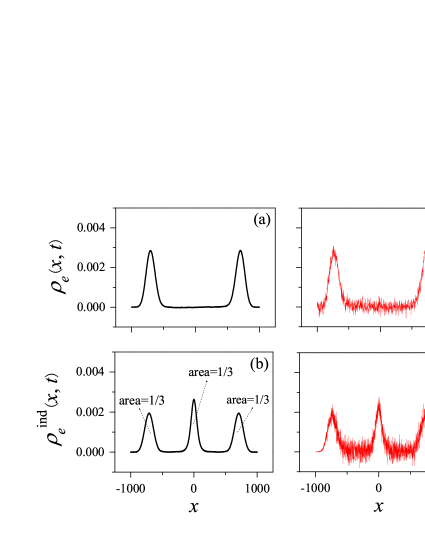
Figure 1: The probability density distribution function of energy obtained by using our correlation function method and the perturbation method with the space variable being, respectively, the coarse-grained space variable and the particle indices. (a)-(d) are for the gas model at $t=400$, obtained by (a)-(b) the correlation function method and (c)-(d) the perturbation method. (e)-(f) are for the FPU model at $t=600$ by using the correlation function method.

For a conserved physical quantity ${\cal A}$, it has been derived in Ref. 18 that the PDF corresponding to a local fluctuation initially located in the $k$th bin, which is specified by $\Delta A_{k}(0)$, can be calculated as

$$\rho_{A}(\Delta x_{k,l},t)=\frac{\langle\Delta A_{l}(t)\Delta A_{k}(0)\rangle}{\langle\Delta A_{k}(0)\Delta A_{k}(0)\rangle}+\frac{1}{N_{b}-1}$$ (7)

if the microcanonical ensemble is considered, and

$$\rho_{A}(\Delta x_{k,l},t)=\frac{\langle\Delta A_{l}(t)\Delta A_{k}(0)\rangle}{\langle\Delta A_{k}(0)\Delta A_{k}(0)\rangle}$$ (8)

if the canonical ensemble is considered. Here $\Delta x_{k,l}$ denotes the displacement from the $k$th bin to the $l$th bin, i.e., $\Delta x_{k,l}\equiv(l-k)b$. For the sake of convenience, in the following we shall use $x$ to denote $\Delta x_{k,l}$ without confusion. The spatiotemporal correlation function defined above gives the causal relation between a local fluctuation and the effects it induces at another position and at a later time, thus it is in essence equivalent to the probability density function that describes the diffusion process of the fluctuation. In order to facilitate numerical simulations, we suggest considering the microcanonical ensemble where all systems are isolated from the environment. Hence one does not have to simulate the environment, which saves greatly the simulation time.

In previous studies, e.g., 14 ; 15 ; 22 ; 23 ; 24 , the authors constantly use the indices of particles to represent the space variable. In particular, the value of ${\cal A}$ of the $k$th particle, denoted by $A_{k}^{{\rm ind}}(t)$, is adopted to represent the density distribution of ${\cal A}$ at the position of $kL/N$, and $\langle\Delta A_{l}^{{\rm ind}}(t)\Delta A_{k}^{\text{i}nd}(0)\rangle$ is assumed to represent the correlation between two positions with a distance of $x=(l-k)L/N$ and a time delay of $t$. In the following, we shall refer to this “coordinate" as the index variable. Although the index represents the mean position of a particle in the equilibrium state, it by no means gives the position of the particle at instant times that is crucial for correctly calculating the spatiotemporal correlation functions. For this reason, Dhar once questioned the effectiveness of the index variable because it may result in large position fluctuations 31 . We find that it is even worse: The deviations caused by using the index variable is not only quantitative, but also qualitative.

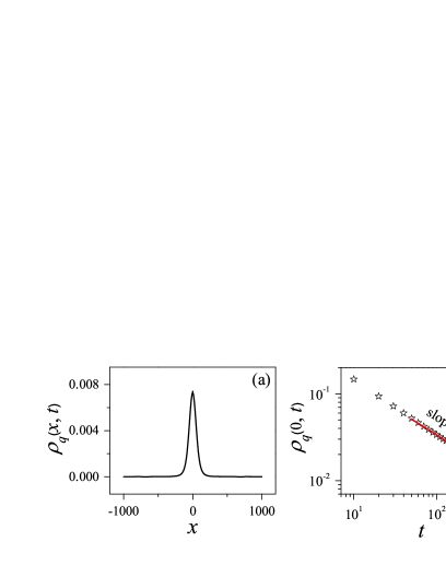
Figure 2: The simulation results of the spatiotemporal correlation function of heat fluctuations, $\rho_{q}(x,t)$, for the 1D gas model. (a) presents a snapshot of $\rho_{q}(x,t)$ at time $t=400$, and (b) shows the time dependence of the height of the center peak of $\rho_{q}(x,t)$. The red solid line in (b) is the best linear fitting of the data for revealing their asymptotic characteristics, suggesting that $\rho_{q}(0,t)\sim t^{-0.60}$. In (c) $\rho_{q}(x,t)t^{\lambda}$ versus $x/t^{\lambda}$ at three different times are compared with the rescaling factor $\lambda=0.60$ obtained via best linear fitting in (b). The fact that three curves overlap perfectly verifies the scaling property of $\rho_{q}(x,t)$.

Taking the energy fluctuations as an example, we show that indeed the index variable may lead to qualitatively wrong results. We denote the spatiotemporal correlation function obtained by using the coarse-grained space variable and the index variable as $\rho_{e}(x,t)$ and $\rho_{e}^{{\rm ind}}(x,t)$, respectively. The 1D gas model is considered first. To prepare an equilibrium gas, the system is efficiently simulated for a sufficient long time by using the event-driven algorithm that employs the heap data structure to identify the collision times 27 . Then $\rho_{e}(x,t)$ and $\rho_{e}^{{\rm ind}}(x,t)$ are calculated with $N=4000$ and $b=1$. Figure 1(a)-(b) show the results. One can see that they are remarkably different: With the coarse-grained space variable, the spatiotemporal correlation function has two peaks, while with the index variable it has three peaks. The two peaks of $\rho_{e}(x,t)$ move outwards with a constant speed $v=1.75$, which can be shown easily to be the sound speed 18 . The two side peaks of $\rho_{e}^{{\rm ind}}(x,t)$ move outwards with the same speed. The center peak of $\rho_{e}^{{\rm ind}}(x,t)$ does not move but broadens as $\Delta w\sim t^{0.67}$, where $\Delta w$ represents its half-height width. It is tempting to think that the two side peaks represent the sound mode and the center peak represents the heat mode, as in the case of the mass fluctuations that gives the dynamic structure factor of the system 4 . But we find the ratio of the area of the center peak to that of the two side peaks equals $1/2$, while it should equal $2$, i.e., the Landau-Placzek ratio 32 ; 33 of an ideal gas, if it characterizes the dynamical structural factor 4 . As will be discussed in the next section, the decaying behavior of the center peak is also different from the heat mode. Therefore, $\rho_{e}^{{\rm ind}}(x,t)$ fails to capture the properties of the heat mode. It is worth noting that the three peak structure has also been reported in other studies of the gas model by using the index variable 14 ; 23 ; 24 .

As mentioned above, diffusion properties can also be investigated directly by observing the evolution of an added perturbation to the system. We find that by applying this method, one can obtain the same results. [See Fig. 1(c)-(d).] In addition, we find that in the 1D FPU model [see Fig. 1(e)-(f)], the qualitative difference between $\rho_{e}(x,t)$ and $\rho_{e}^{{\rm ind}}(x,t)$ is also obvious 18 . These results suggest clearly that the position of a particle at instant times cannot be approximated by its equilibrium position in order to correctly calculate spatiotemporal correlation functions.

IV Results and Discussions

In Fig. 1(a), it is clearly shown that the energy fluctuations transport ballistically in the 1D gas model, implying that the mean square displacement of the transported energy increases in time as $\langle x^{2}(t)\rangle\sim t^{2}$. On the other hand, the heat conduction properties of this model have been extensively studied in the literatures 25 ; 26 ; 27 . It has been found that the heat conductivity $\kappa$ diverges with the system size $L$ as $\kappa\sim L^{\alpha}$ with $\alpha=1/3$ 27 ; 28 ; 29 ; 30 , suggesting that heat diffuses in a supperdiffusive manner rather than ballistically. Therefore, energy diffusion and heat conduction do not fall into the same anomalous class. We then calculate the PDF of heat fluctuations, i.e., $\rho_{q}(x,t)$, following Eq. (2) and present the results in Fig. 2. It can be seen that the profile of $\rho_{q}(x,t)$ is completely different from that of energy fluctuations, $\rho_{e}(x,t)$ [see Fig. 1(a)]; the former has only one single peak. This outstanding feature has been reported in ref. 18 , but here we perform the simulation with a larger system size of $N=4096$ which allows us to measure the decaying rate of $\rho_{q}(x,t)$ more accurate. As presented in Fig. 2(b), we obtain that the height of the peak of $\rho_{q}(x,t)$ goes as $h=\rho_{q}(0,t)\sim t^{-\lambda}$ with $\lambda=0.60$. As heat is a conserved quantity, the peak of $\rho_{q}(x,t)$ must keep its area unchange, and as a consequence its half-height width should broaden as $\Delta w\sim t^{-0.60}$. As such $\rho_{q}(x,t)$ at different time may be rescaled onto a common function. This is confirmed by our study presented in Fig. 2(c): $\rho_{q}(x,t)$ is indeed invariant upon rescaling $x\rightarrow t^{\lambda}x$ so that $t^{\lambda}\rho_{q}(x,t)=t_{0}^{\lambda}\rho_{q}(x_{0},t_{0})$ for $x=({t}/{t_{0}})^{\lambda}x_{0}$ with scaling factor $\lambda=0.60$.

Figure 3: The spatiotemporal correlation function of local energy current $C_{e}(x,t)$ (a) and of local heat current $C_{q}(x,t)$ (b) at time $t=400$ for the 1D gas model $N$=3000. In (c), the autocorrelation function of the globe energy current $\langle J_{e}(t)J_{e}(0)\rangle$ (black solid line) is compared with $\int C_{e}(x,t)dx$ (blue open squares) and $\int C_{q}(x,t)dx$ (red solid triangles). The three sets of data fall onto the same curve upon proper shifts in vertical direction. $N$=512.

This result confirms for the first time that the relaxation of the heat mode follows the scaling law with $\lambda=3/5$ as predicted by the hydrodynamic mode-coupling theory 34 . This scaling property implies that $\rho_{q}(x,t)$ relaxes as $\langle x^{2}(t)\rangle=\langle x_{0}^{2}(t_{0})\rangle(\frac{t}{t_{0}})^{2\lambda}$; i.e., heat fluctuations diffuse in a power law $\langle x^{2}(t)\rangle\sim t^{\beta}$ with the diffusion exponent $\beta=2\lambda$ 18 . We obtain $\beta=1.20$ accordingly, suggesting that heat diffusion is superdiffusive, in clear contrast with energy diffusion which is ballistic. More important and interesting, by combining $\beta=1.20$ obtained here and $\alpha=1/3$ obtained in previous analytical and numerical studies 27 ; 28 ; 29 ; 30 , we find they follow perfectly the general formula proposed by Li and Wang 16 that trying to connect energy diffusion (should be heat diffusion instead) and heat conduction in 1D systems.

We would like to point out that the center peak of $\rho_{e}^{{\rm ind}}(x,t)$ [see Fig. 1(a)] is also invariant upon the rescaling but with $\lambda=0.67$ instead, which implies $\beta=1.34$. One may notice that the formula $\alpha=\beta-1$ correctly describes the relation of energy diffusion and heat conduction in this case, as pointed in Ref. 14 ; 15 . We can therefore conclude that this is a consequence by improperly replacing the space variable with the particle indices.

Finally, we study the relaxation behavior of local energy current and local heat current. We set the total momentum of the system to be zero. As having been pointed out in Ref. 18 , the global energy current always equals the globe heat current, but this fact does not imply the properties of local heat current and local energy current are also identical. Figure 3(a)-(b) show the spatiotemporal correlation functions of local energy current $C_{e}(x,t)=\langle j_{l}^{e}(t)j_{k}^{e}(0)\rangle$ and that of local heat current $C_{q}(x,t)=\langle j_{l}^{q}(t)j_{k}^{q}(0)\rangle$. Here $x=(l-k)L/N$, ( the size of a bin is $b=L/N$ ), the local energy current is defined as $j_{l}^{e}(t)=\sum_{k:x_{k}\in l{\rm th\leavevmode\nobreak\ bin}}m_{k}v_{k}^{3}/2$, and the local heat current is obtained by substituting $j_{l}^{e}(t)$ into Eq. (3). It can be seen that $C_{e}(x,t)$ and $C_{q}(x,t)$ have remarkably different features: The former has a global negative bias, and its two peaks moving oppositely at the sound speed. The latter is more complicated. There are two pulses which look like a negative Mexican hat wavelet and move outwards at the sound speed, but there is no global bias. Instead, there is a dip at the origin. Therefore, the properties of $C_{q}(x,t)$ can not be probed by studying $C_{e}(x,t)$, and vice versa.

The globe energy current $J_{e}(t)=\sum_{k}j_{k}^{e}(t)$. One has $\langle J_{e}(t)J_{e}(0)\rangle=\langle\sum_{k}j_{k}^{e}(0)\sum_{l}j_{l}^{e}(t)\rangle\propto\langle j_{k}^{e}(0)\sum_{l}j_{l}^{e}(t)\rangle$ for any index $k$ because of the homogeneity of the system. In other words, $\langle J_{e}(t)J_{e}(0)\rangle\propto\int C_{e}(x,t)dx$. Because $J_{e}(t)=J_{q}(t)$ as a result of the null total momentum, we have $\int C_{e}(x,t)dx\propto\int C_{q}(x,t)dx$. This result implies that though the relaxation behaviors of local heat current and local energy current are different, their integrals decay in the same way, which is also confirmed by direct simulation results shown in Fig. 3(c).

V Summary

We demonstrate that in 1D systems, using the particle indices as the space variable may result in qualitative deviations in probing the diffusion properties, and hence should be abandoned. Instead, the coarse-grained space variable is a correct and practical choice. By taking advantage of it, we have verified that in the 1D gas model, heat diffusion and heat conduction, rather than energy diffusion and heat conduction, can be connected by the formula $\alpha=2-2/\beta$ 16 accurately, rather than by that proposed in 17 . Our analysis has also shown that energy diffusion and heat conduction follows $\alpha=\beta-1$ as observed in Ref. 14 ; 15 may be a misunderstanding caused by misusing the particle indices as the space variable. We emphasize that the position of a particle at instant times cannot be approximated by its equilibrium position in probing spatiotemporal correlation functions of a system.

In addition, in the case of null total momentum, the globe energy current and the globe heat current are found to be the same. But local energy currents are different from local heat currents. The relaxation behavior of the former is significantly different from that of the latter as well. We conclude that in general, the relaxation and transport properties of heat can not be identified with those of energy.

- (1) Landau L D, Lifshitz E M. Course of Theoretical Physics, Vol. VI: Fluid Mechanics. New York: Pergamon Press, 1959
- (2) Kadanoff L P and Martin P C. Hydrodynamic equations and correlation functions. Ann Phys (N.Y.), 1963, 24: 419
- (3) Forster D. Hydrodynamic Fluctuations, Broken Symmetry, and Correlation Functions. New York: Benjamin, 1975
- (4) Hansen J P, McDonald I R. Theory of Simple Liquids, 3rd ed. London: Academic Press, 2006
- (5) Kim P, Shi L, Majumdar A, et al. Thermal transport measurements of individual multiwalled nanotubes. Phys Rev Lett, 2001, 87: 215502
- (6) Geim A K,Novoselov k s. The rise of graphene. Nature Mater, 2007, 6: 183-191
- (7) Bonetto F, Lebowitz J L, Ray-Bellet L. Fourier’s law: a challenge for theorists, in Mathematical Physics 2000, edited by A. Fokas et al. London: Imperial College Press, 2000
- (8) Lepri S, Livi R, Politi A. Thermal conduction in classical low-dimensional lattices. Phys Rep, 2003, 377: 1
- (9) Livi R, Lepri S. Heat in one dimension. Nature, 2003, 421: 327
- (10) Buchanan M. Heated debate in different dimensions. Nature Phys, 2005, 1: 71
- (11) Dhar A. Heat transport in low-dimensional systems. Adv Phys, 2008, 57: 457
- (12) Chang C W, Okawa D, Garcia H, et al. Breakdown of Fourier’s law in nanotube thermal conductors. Phys Rev Lett, 2008, 101: 075903
- (13) Li N, Ren J,Wang L, et al. Colloquium: Phononics: Manipulating heat flow with electronic analogs and beyond. Rev Mod Phys, 2012, 84: 1045-1066
- (14) Cipriani P, Denisov S, Politi A. From anomalous energy diffusion to Lï¿œvy walks and heat conductivity in one-dimensional systems. Phys Rev Lett, 2005, 94: 244301
- (15) Zhao H. Identifying diffusion processes in one-dimensional lattices in thermal equilibrium. Phys Rev Lett, 2006, 96: 140602
- (16) Li B,Wang J. Anomalous heat conduction and anomalous diffusion in one-dimensional systems. Phys Rev Lett, 2003, 91: 044301
- (17) Denisov S, Klafter J, Urbakh M. Dynamical heat channels. Phys Rev Lett, 2003, 91: 194301
- (18) Chen S, Zhang Y, Wang J, et al. Diffusion of heat, energy, momentum, and mass in one-dimensional systems. Phys Rev E, 2013, 87: 032153
- (19) Hwang P, Zhao H. Methods of exploring energy diffusion in lattices with finite temperature. Preprint, 2011, arXiv:1106.2866
- (20) Zavt G S, Wagner M, Lutze A. Anderson localization and solitonic energy transport in one-dimensional oscillatory systems. Phys Rev E, 1993, 47: 4108
- (21) Li B, Casati G, Wang J, et al. Fourier law in the alternate-mass hard-core potential chain. Phys Rev Lett, 2004, 92: 254301
- (22) Li B, Wang J, Wang L, et al. Anomalous heat conduction and anomalous diffusion in nonlinear lattices, single walled nanotubes, and billiard gas channels. Chaos, 2005, 15: 015121
- (23) Delfini L, Denisov S, Lepri S, et al. Energy diffusion in hard-point systems. Eur Phys J Special Topics, 2007, 146: 21
- (24) Zaburdaev V S, Denisov S, Hï¿œnggi P. Perturbation spreading in many-particle systems: a random walk approach. Phys Rev Lett, 2011, 106: 180601
- (25) Dhar A. Heat conduction in a one-dimensional gas of elastically colliding particles of unequal masses. Phys Rev Lett, 2001, 86: 3554
- (26) Savin A V, Tsironis G P, Zolotaryuk A V. Heat conduction in one-dimensional systems with hard-point interparticle interactions. Phys Rev Lett, 2002, 88: 154301
- (27) Grassberger P, Nadler W, Yang L. Heat conduction and entropy production in a one-dimensional hard-particle gas. Phys Rev Lett, 2002, 89: 180601
- (28) Narayan O, Ramaswamy S. Anomalous heat conduction in one-dimensional momentum-conserving systems. Phys Rev Lett, 2002, 89: 200601
- (29) Delfini L, Lepri S, Livi R, et al. Self-consistent mode-coupling approach to one-dimensional heat transport. Phys Rev E, 2006, 73: 060201
- (30) Delfini L, Lepri S, Livi R, et al. Anomalous kinetics and transport from 1D self-consistent mode-coupling theory. J Stat Mech 2007, P02007
- (31) Dhar A. Comment on "Simple one-dimensional model of heat conduction which obeys Fourier’s law". Phys Rev Lett, 2002, 88: 249401
- (32) Landau L D, Lifshitz E M. Theoretical Physics, Vol. VIII: Electrodynamics of Continuous Media. Oxford: Pergamon Press, 1984
- (33) Cummins H Z, Gammon R W. Rayleigh and Brillouin scattering in liquids: the Landau-Placzek ratio. J Chem Phys, 1966, 44:2785
- (34) van Beijeren H. Exact results for anomalous transport in one-dimensional Hamiltonian systems. Phys Rev Lett, 2012, 108: 180601