Entropic uncertainty and measurement reversibility

Abstract

The entropic uncertainty relation with quantum side information (EUR-QSI) from [Berta et al., Nat. Phys. 6, 659 (2010)] is a unifying principle relating two distinctive features of quantum mechanics: quantum uncertainty due to measurement incompatibility, and entanglement. In these relations, quantum uncertainty takes the form of preparation uncertainty where one of two incompatible measurements is applied. In particular, the “uncertainty witness” lower bound in the EUR-QSI is not a function of a post-measurement state. An insightful proof of the EUR-QSI from [Coles et al., Phys. Rev. Lett. 108, 210405 (2012)] makes use of a fundamental mathematical consequence of the postulates of quantum mechanics known as the non-increase of quantum relative entropy under quantum channels. Here, we exploit this perspective to establish a tightening of the EUR-QSI which adds a new state-dependent term in the lower bound, related to how well one can reverse the action of a quantum measurement. As such, this new term is a direct function of the post-measurement state and can be thought of as quantifying how much disturbance a given measurement causes. Our result thus quantitatively unifies this feature of quantum mechanics with the others mentioned above. We have experimentally tested our theoretical predictions on the IBM Quantum Experience and find reasonable agreement between our predictions and experimental outcomes.

LABEL:FirstPage1 LABEL:LastPage#110

I Introduction

The uncertainty principle is one of the cornerstones of modern physics, providing a striking separation between classical and quantum mechanics H27 . It is routinely used to reason about the behavior of quantum systems, and in recent years, an information-theoretic refinement of it that incorporates quantum side information has been helpful for witnessing entanglement and in establishing the security of quantum key distribution BCCRR10 . This latter refinement, known as the entropic uncertainty relation with quantum side information (EUR-QSI), is the culmination of a sequence of works spanning many decades R29 ; hirschman57 ; bial1 ; beckner75 ; D83 ; K87 ; MU88 ; KP02 ; christandl05 ; RB09  and is the one on which we focus here.

Tripartite uncertainty relations. There are two variations of the EUR-QSI BCCRR10 , one for tripartite and one for bipartite scenarios. For the first, let $\rho_{ABE}$ denote a tripartite quantum state shared between Alice, Bob, and Eve, and let $\mathbb{X}\equiv\{P_{A}^{x}\}$ and $\mathbb{Z}=\{Q_{A}^{z}\}$ be projection-valued measures (PVMs) that can be performed on Alice’s system (note that considering PVMs implies statements for the more general positive operator-valued measures, by invoking the Naimark extension theorem Naimark40 ). If Alice chooses to measure $\mathbb{X}$, then the post-measurement state is as follows:

$$\sigma_{XBE} \equiv\sum_{x}|x\rangle\langle x|_{X}\otimes\sigma_{BE}^{x}\qquad\mathrm{where}$$

$$\sigma_{BE}^{x} \equiv\operatorname{Tr}_{A}\{(P_{A}^{x}\otimes I_{BE})\rho_{ABE}\}.$$ (1)

Similarly, if Alice instead chooses to measure $\mathbb{Z}$, then the post-measurement state is

$$\omega_{ZBE} \equiv\sum_{z}|z\rangle\langle z|_{Z}\otimes\omega_{BE}^{z}\qquad\mathrm{where}$$

$$\omega_{BE}^{z} \equiv\operatorname{Tr}_{A}\{(Q_{A}^{z}\otimes I_{BE})\rho_{ABE}\}.$$ (2)

In the above, $\{|x\rangle_{X}\}_{x}$ and $\{|z\rangle_{Z}\}_{z}$ are orthonormal bases that encode the classical outcome of the respective measurements. The following tripartite EUR-QSI in (3) quantifies the trade-off between Bob’s ability to predict the outcome of the $\mathbb{X}$ measurement with the help of his quantum system $B$ and Eve’s ability to predict the outcome of the $\mathbb{Z}$ measurement with the help of her system $E$:

$$H(X|B)_{\sigma}+H(Z|E)_{\omega}\geq-\log c,$$ (3)

where here and throughout we take the logarithm to have base two. In the above,

$$H(F|G)_{\tau}\equiv H(FG)_{\tau}-H(G)_{\tau}=H(\tau_{FG})-H(\tau_{G})$$ (4)

denotes the conditional von Neumann entropy of a state $\tau_{FG}$, with $H(\tau)\equiv-\operatorname{Tr}\{\tau\log\tau\}$, and the parameter $c$ captures the incompatibility of the $\mathbb{X}$ and $\mathbb{Z}$ measurements:

$$c\equiv\max_{x,z}\|P_{A}^{x}Q_{A}^{z}\|_{\infty}^{2}\in[0,1].$$ (5)

The conditional entropy $H(F|G)_{\tau}$ is a measure of the uncertainty about system $F$ from the perspective of someone who possesses system $G$, given that the state of both systems is $\tau_{FG}$. The uncertainty relation in (3) thus says that if Bob can easily predict $X$ given $B$ (i.e., $H(X|B)$ is small) and the measurements are incompatible, then it is difficult for Eve to predict $Z$ given $E$ (i.e., $H(Z|E)$ is large). As such, (5) at the same time captures measurement incompatibility and the monogamy of entanglement monogamyGames . A variant of (3) in terms of the conditional min-entropy TR11 can be used to establish the security of quantum key distribution under particular assumptions TLGR12 ; TL15 .

The EUR-QSI in (3) can be summarized informally as a game involving a few steps. To begin with, Alice, Bob, and Eve are given a state $\rho_{ABE}$. Alice then flips a coin to decide whether to measure $\mathbb{X}$ or $\mathbb{Z}$. If she gets heads, she measures $\mathbb{X}$ and tells Bob that she did so. Bob then has to predict the outcome of her $\mathbb{X}$ measurement and can use his quantum system $B$ to help do so. If Alice gets tails, she instead measures $\mathbb{Z}$ and tells Eve that she did so. In this case, Eve has to predict the outcome of Alice’s $\mathbb{Z}$ measurement and can use her quantum system $E$ as an aid. There is a trade-off between their ability to predict correctly, which is captured by (3).

Bipartite uncertainty relations. We now recall the second variant of the EUR-QSI from BCCRR10 . Here we have a bipartite state $\rho_{AB}$ shared between Alice and Bob and again the measurements $\mathbb{X}$ and $\mathbb{Z}$ mentioned above. Alice chooses to measure either $\mathbb{X}$ or $\mathbb{Z}$, leading to the respective post-measurement states $\sigma_{XB}$ and $\omega_{ZB}$ defined from (1) and (2) after taking a partial trace over the $E$ system. The following EUR-QSI in (6) quantifies the trade-off between Bob’s ability to predict the outcome of the $\mathbb{X}$ or $\mathbb{Z}$ measurement:

$$H(Z|B)_{\omega}+H(X|B)_{\sigma}\geq-\log c+H(A|B)_{\rho},$$ (6)

where the incompatibility parameter $c$ is defined in (5) and the conditional entropy $H(A|B)_{\rho}$ is a signature of both the mixedness and entanglement of the state $\rho_{AB}$. For (6) to hold, we require the technical condition that the $\mathbb{Z}$ measurement be a rank-one measurement CYZ11 (however see also FL13 ; furrer13 for a lifting of this condition). The EUR-QSI in (6) finds application in witnessing entanglement, as discussed in BCCRR10 .

The uncertainty relation in (6) can also be summarized informally as a game, similar to the one discussed above. Here, we have Alice choose whether to measure $\mathbb{X}$ or $\mathbb{Z}$. If she measures $\mathbb{X}$, she informs Bob that she did so, and it is his task to predict the outcome of the $\mathbb{X}$ measurement. If she instead measures $\mathbb{Z}$, she tells Bob, and he should predict the outcome of the $\mathbb{Z}$ measurement. In both cases, Bob is allowed to use his quantum system $B$ to help in predicting the outcome of Alice’s measurement. Again there is generally a trade-off between how well Bob can predict the outcome of the $\mathbb{X}$ or $\mathbb{Z}$ measurement, which is quantified by (6). The better that Bob can predict the outcome of either measurement, the more entangled the state $\rho_{AB}$ is.

II Main result

The main contribution of the present paper is to refine and tighten both of the uncertainty relations in (3) and (6) by employing a recent result from Junge15 (see also W15 ; Sutter15 ; SBT16 ). This refinement adds a term involving measurement reversibility, next to the original trade-offs in terms of measurement incompatibility and entanglement. An insightful proof of the EUR-QSIs above makes use of an entropy inequality known as the non-increase of quantum relative entropy Lindblad1975 ; U77 . This entropy inequality is fundamental in quantum physics, providing limitations on communication protocols W13 and thermodynamic processes S12 . The main result of Junge15 ; W15 ; Sutter15 ; SBT16 offers a strengthening of the non-increase of quantum relative entropy, quantifying how well one can recover from the deleterious effects of a noisy quantum channel. Here we apply the particular result from Junge15 to establish a tightening of both uncertainty relations in (3) and (6) with a term related to how well one can “reverse” an additional $\mathbb{X}$ measurement performed on Alice’s system at the end of the uncertainty game, if the outcome of the $\mathbb{X}$ measurement and the $B$ system are available. The upshot is an entropic uncertainty relation which incorporates measurement reversibility in addition to quantum uncertainty due to measurement incompatibility, and entanglement, thus unifying several genuinely quantum features into a single uncertainty relation.

In particular, we establish the following refinements of (3) and (6):

$$H(Z|E)_{\omega}+H(X|B)_{\sigma} \geq-\log c-\log f,$$ (7)

$$H(Z|B)_{\omega}+H(X|B)_{\sigma} \geq-\log c-\log f+H(A|B)_{\rho},$$ (8)

where $c$ is defined in (5),

$$f\equiv F(\rho_{AB},\mathcal{R}_{XB\rightarrow AB}(\sigma_{XB})),$$ (9)

and in (8) we need the projective $\mathbb{Z}$ measurement to be a rank-one measurement (i.e., $Q_{A}^{z}=|z\rangle\langle z|$). In addition to the measurement incompatibility $c$, the term $f$ quantifies the disturbance caused by one of the measurements, in particular, how reversible such a measurement is. $F(\rho_{1},\rho_{2})\equiv\|\sqrt{\rho_{1}}\sqrt{\rho_{2}}\|_{1}^{2}$ denotes the quantum fidelity between two density operators $\rho_{1}$ and $\rho_{2}$ U73 , and $\mathcal{R}_{XB\rightarrow AB}$ is a recovery quantum channel with input systems $XB$ and output systems $AB$. Appendix A details a proof for (7) and (8). In Section IV, we discuss several simple exemplary states and measurements to which (8) applies, and in Section V, we detail the results of several experimental tests of the theoretical predictions, finding reasonable agreement between the experimental results and our predictions.

In the case that the $\mathbb{Z}$ measurement has the form $\{Q_{A}^{z}=|z\rangle\langle z|_{A}\}_{z}$ for an orthonormal basis $\{|z\rangle_{A}\}_{z}$, the action of the recovery quantum channel $\mathcal{R}_{XB\rightarrow AB}$ on an arbitrary state $\xi_{XB}$ is explicitly given as follows (see Appendix B for details):

$$\mathcal{R}_{XB\rightarrow AB}(\xi_{XB})=\sum_{z,x,z^{\prime}}|z\rangle\langle z|_{A}P_{A}^{x}|z^{\prime}\rangle\langle z^{\prime}|_{A}\otimes\mathcal{R}_{XB\rightarrow B}^{x,z,z^{\prime}}(\xi_{XB}),$$ (10)

where

$$\mathcal{R}_{XB\rightarrow B}^{x,z,z^{\prime}}(\xi_{XB})\equiv\int_{-\infty}^{\infty}dt\ p(t)\left(\omega_{B}^{z}\right)^{\frac{1-it}{2}}\left(\theta_{B}^{x}\right)^{\frac{-1+it}{2}}\operatorname{Tr}_{X}\{|x\rangle\langle x|_{X}(\xi_{XB})\}\left(\theta_{B}^{x}\right)^{\frac{-1-it}{2}}(\omega_{B}^{z^{\prime}})^{\frac{1+it}{2}},$$ (11)

with the probability density $p(t)\equiv\frac{\pi}{2}(\cosh(\pi t)+1)^{-1}$. (Note that $\mathcal{R}_{XB\rightarrow B}^{x,z,z^{\prime}}$ is not a channel—we are merely using this notation as a shorthand.) In the above, $\theta_{XB}$ is the state resulting from Alice performing the $\mathbb{Z}$ measurement, following with the $\mathbb{X}$ measurement, and then discarding the outcome of the $\mathbb{Z}$ measurement:

$$\theta_{XB} \equiv\sum_{x}|x\rangle\langle x|_{X}\otimes\theta_{B}^{x}\quad\mathrm{with}$$

$$\theta_{B}^{x} \equiv\sum_{z}\langle z|P_{A}^{x}|z\rangle\ \omega^{z}_{B}.$$ (12)

For this case, $\omega^{z}_{B}$ from (2) reduces to $\omega^{z}_{B}=(\langle z|_{A}\otimes I_{B})\rho_{AB}(|z\rangle_{A}\otimes I_{B})$. As one can readily check by plugging into (10), the recovery channel $\mathcal{R}$ has the property that it perfectly reverses an $\mathbb{X}$ measurement if it is performed after a $\mathbb{Z}$ measurement:

$$\mathcal{R}_{XB\rightarrow AB}(\theta_{XB})=\sum_{z}|z\rangle\langle z|_{A}\otimes\omega^{z}_{B}.$$ (13)

The fidelity $F(\rho_{AB},\mathcal{R}_{XB\rightarrow AB}(\sigma_{XB}))$ thus quantifies how much disturbance the $\mathbb{X}$ measurement causes to the original state $\rho_{AB}$ in terms of how well the recovery channel $\mathcal{R}$ can reverse the process. We note that there is a trade-off between reversing the $\mathbb{X}$ measurement whenever it is greatly disturbing $\rho_{AB}$ and meeting the constraint in (13). Since the quantum fidelity always takes a value between zero and one, it is clear that (7) and (8) represent a state-dependent tightening of (3) and (6), respectively.

III Interpretation

It is interesting to note that just as the original relation in (6) could be used to witness entanglement, the new relation can be used to witness both entanglement and recovery from measurement, as will be illustrated using the examples below. That is, having low conditional entropy for both measurement outcomes constitutes a recoverability witness, when given information about the entanglement.

We recalled above the established “uncertainty games” in order to build an intuition for (3) and (6). In order to further understand the refinements in (7) and (8), we could imagine that after either game is completed, we involve another player Charlie. Regardless of which measurement Alice performed in the original game, she then performs an additional $\mathbb{X}$ measurement. Bob sends his quantum system $B$ to Charlie, and Alice sends the classical outcome of the final $\mathbb{X}$ measurement to Charlie. It is then Charlie’s goal to “reverse” the $\mathbb{X}$ measurement in either of the scenarios above, and his ability to do so is limited by the uncertainty relations in (7) and (8). Figure 1 depicts this game. In the case that (a) Alice performed an $\mathbb{X}$ measurement in the original game, the state that Charlie has is $\sigma_{XB}$. In the case that (b) Alice performed a $\mathbb{Z}$ measurement in the original game, then the state that Charlie has is $\theta_{XB}$. Not knowing which state he has received, Charlie can perform the recovery channel $\mathcal{R}$ and be guaranteed to restore the state to

$$\sum_{z}|z\rangle\langle z|\otimes\big{(}\langle z|\otimes I_{B}\big{)}\rho_{AB}\big{(}|z\rangle\otimes I_{B}\big{)}$$ (14)

in the case that (b) occurred, while having a performance limited by (7) or (8) in the case that (a) occurred.

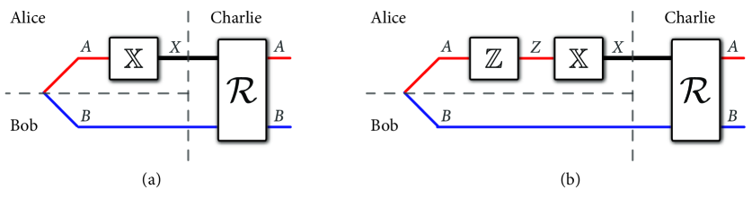
Figure 1: Measurement reversibility game. How well can Charlie reverse the action of the $\mathbb{X}$ measurement in either scenario (a) or (b)? The quantities in (7) and (8) other than $f$ constitute a “recoverability witness,” quantifying Charlie’s ability to do so.

IV Examples

It is helpful to examine some examples in order to build an intuition for our refinements of the EUR-QSIs. Here we focus on the bipartite EUR-QSI in (8) and begin by evaluating it for some “minimum uncertainty states” CYZ11 (see also CCYZ12 ). These are states for which the original uncertainty relation in (6) is already tight, i.e., an equality. Later, we will consider the case of a representative “maximum uncertainty state,” that is, a state for which the original uncertainty relation (6) is maximally non-tight. This last example distinguishes our new contribution in (8) from the previously established bound in (6).

For all of the forthcoming examples, we take the $\mathbb{X}$ measurement to be Pauli $\sigma_{X}$ and the $\mathbb{Z}$ measurement to be Pauli $\sigma_{Z}$, which implies that $-\log c=1$. We define the “BB84” states $|0\rangle$, $|1\rangle$, $|+\rangle$, and $|-\rangle$ from the following relations:

$$\sigma_{Z}|0\rangle=|0\rangle,\qquad\sigma_{Z}|1\rangle=(-1)|1\rangle,\qquad\sigma_{X}|+\rangle=|+\rangle,\qquad\sigma_{X}|-\rangle=(-1)|-\rangle.$$ (15)

So this means that the $\mathbb{X}$ and $\mathbb{Z}$ measurements have the following respective implementations as quantum channels acting on an input $\xi$:

$$\xi \rightarrow\langle+|_{A}\xi|+\rangle_{A}|0\rangle\langle 0|_{X}+\langle-|_{A}\xi|-\rangle_{A}|1\rangle\langle 1|_{X},$$ (16)

$$\xi \rightarrow\langle 0|_{A}\xi|0\rangle_{A}|0\rangle\langle 0|_{Z}+\langle 1|_{A}\xi|1\rangle_{A}|1\rangle\langle 1|_{Z}.$$ (17)

IV.1 Minimum uncertainty states

IV.1.1 $X$ eigenstate on system $A$

First suppose that $\rho_{AB}=|+\rangle\langle+|_{A}\otimes\pi_{B}$, where $\pi$ is the maximally mixed state. In this case, Bob’s system $B$ is of no use to help predict the outcome of a measurement on the $A$ system because the systems are in a product state. Here we find by direct calculation that $H(A|B)_{\rho}=0$, $H(X|B)_{\sigma}=0$, and $H(Z|B)_{\omega}=1$. By (8), this then implies that there exists a recovery channel $\mathcal{R}^{(1)}$ such that (13) is satisfied and, given that $\sigma_{XB}=|0\rangle\langle 0|_{X}\otimes\pi_{B}$, we also have the perfect recovery

$$\mathcal{R}_{XB\rightarrow AB}^{(1)}\big{(}|0\rangle\langle 0|_{X}\otimes\pi_{B}\big{)}=|+\rangle\langle+|_{A}\otimes\pi_{B}.$$ (18)

To determine the recovery channel $\mathcal{R}^{(1)}$, consider that

$$\sum_{z}|z\rangle\langle z|_{Z}\otimes\omega_{B}^{z}=\pi_{Z}\otimes\pi_{B},\qquad\sum_{x}|x\rangle\langle x|_{X}\otimes\theta_{B}^{x}=\pi_{X}\otimes\pi_{B},$$ (19)

with the states on the left in each case defined in (2) and (12), respectively. Plugging into (10), we find that the recovery channel in this case is given explicitly by

$$\mathcal{R}_{XB\rightarrow AB}^{(1)}(\xi_{XB})=|+\rangle\langle+|_{A}\otimes\operatorname{Tr}_{X}\{|0\rangle\langle 0|_{X}\xi_{XB}\}+|-\rangle\langle-|_{A}\otimes\operatorname{Tr}_{X}\{|1\rangle\langle 1|_{X}\xi_{XB}\},$$ (20)

so that we also see that

$$\mathcal{R}_{XB\rightarrow AB}^{(1)}(\pi_{X}\otimes\pi_{B})=\pi_{A}\otimes\pi_{B}.$$ (21)

IV.1.2 $Z$ eigenstate on system $A$

The situation in which $\rho_{AB}=|0\rangle\langle 0|_{A}\otimes\pi_{B}$ is similar in some regards, but the recovery channel is different—i.e., we have by direct calculation that $H(A|B)_{\rho}=0$, $H(X|B)_{\sigma}=1$, and $H(Z|B)_{\omega}=0$, which implies the existence of a different recovery channel $\mathcal{R}^{(2)}$ such that (13) is satisfied, and given that $\sigma_{XB}=\pi_{X}\otimes\pi_{B}$, we also have the perfect recovery

$$\mathcal{R}_{XB\rightarrow AB}^{(2)}\big{(}\pi_{X}\otimes\pi_{B}\big{)}=|0\rangle\langle 0|_{A}\otimes\pi_{B}.$$ (22)

To determine the recovery channel $\mathcal{R}^{(2)}$, consider that

$$\sum_{z}|z\rangle\langle z|_{Z}\otimes\omega_{B}^{z}=|0\rangle\langle 0|_{Z}\otimes\pi_{B},\qquad\sum_{x}|x\rangle\langle x|_{X}\otimes\theta_{B}^{x}=\pi_{X}\otimes\pi_{B},$$ (23)

with the states on the left in each case defined in (2) and (12), respectively. Plugging into (10), we find that the recovery channel in this case is given explicitly by

$$\mathcal{R}_{XB\rightarrow AB}^{(2)}(\xi_{XB})=|0\rangle\langle 0|_{A}\otimes\operatorname{Tr}_{X}\{\xi_{XB}\}.$$ (24)

IV.1.3 Maximally entangled state on systems $A$ and $B$

Now suppose that $\rho_{AB}=|\Phi\rangle\langle\Phi|_{AB}$ is the maximally entangled state, where $|\Phi\rangle_{AB}\equiv(|00\rangle_{AB}+|11\rangle_{AB})/\sqrt{2}$. In this case, we have that both $H(X|B)_{\sigma}=0$ and $H(Z|B)_{\omega}=0$, but the conditional entropy is negative: $H(A|B)_{\rho}=-1$. So here again we find the existence of a recovery channel $\mathcal{R}^{(3)}$ such that (13) is satisfied, and given that $\sigma_{XB}=(|0+\rangle\langle 0+|_{XB}+|1-\rangle\langle 1-|_{XB})/2$, we also have the perfect recovery

$$\mathcal{R}_{XB\rightarrow AB}^{(3)}\Big{(}\big{(}|0+\rangle\langle 0+|_{XB}+|1-\rangle\langle 1-|_{XB}\big{)}/2\Big{)}=|\Phi\rangle\langle\Phi|_{AB}.$$ (25)

To determine the recovery channel $\mathcal{R}^{(3)}$, consider that

$$\sum_{z}|z\rangle\langle z|_{Z}\otimes\omega_{B}^{z} =\frac{1}{2}\left(|0\rangle\langle 0|_{Z}\otimes|0\rangle\langle 0|_{B}+|1\rangle\langle 1|_{Z}\otimes|1\rangle\langle 1|_{B}\right),$$ (26)

$$\sum_{x}|x\rangle\langle x|_{X}\otimes\theta_{B}^{x} =\pi_{X}\otimes\pi_{B},$$ (27)

with the states on the left in each case defined in (2) and (12), respectively. Plugging into (10), we find that the recovery channel in this case is given explicitly by

$$\mathcal{R}_{XB\rightarrow AB}^{(3)}(\xi_{XB})=\sum_{z,z^{\prime},x\in\left\{0,1\right\}}\left(-1\right)^{x(z+z^{\prime})}|z\rangle\langle z^{\prime}|_{A}\otimes|z\rangle\langle z^{\prime}|_{B}\operatorname{Tr}\{|x\rangle\langle x|_{X}\otimes|z^{\prime}\rangle\langle z|_{B}\xi_{XB}\},$$ (28)

i.e., with the following Kraus operators:

$$\left\{\sum_{z}\left(-1\right)^{xz}\left(|z\rangle_{A}\otimes|z\rangle_{B}\right)\left(\langle x|_{X}\otimes\langle z|_{B}\right)\right\}_{x}.$$ (29)

These Kraus operators give the recovery map $\mathcal{R}_{XB\rightarrow AB}^{(3)}$ the interpretation of 1) measuring the $X$ register and 2) coherently copying the contents of the $B$ register to the $A$ register along with an appropriate relative phase. It can be implemented by performing a controlled-NOT gate from $B$ to $A$, followed by a controlled-phase gate on $X$ and $B$ and a partial trace over system $X$.

Remark 1

All of the examples mentioned above involve a perfect recovery or a perfect reversal of the $\mathbb{X}$ measurement. This is due to the fact that the bound in (6) is saturated for these examples. However, the refined inequality in (8) allows to generalize these situations to the approximate case, in which $\rho_{AB}$ is nearly indistinguishable from the states given above. It is then the case that the equalities in (18)–(25) become approximate equalities, with a precise characterization given by (8).

IV.2 Maximum uncertainty states

We now investigate the extreme opposite situation, when the bound in (6) is far from being saturated but its refinement in (8) is saturated. Let $\rho_{AB}=|+_{Y}\rangle\langle+_{Y}|_{A}\otimes\pi_{B}$, where $|+_{Y}\rangle$ is defined from the relation $\sigma_{Y}|+_{Y}\rangle=|+_{Y}\rangle$. In this case, we find that both $H(X|B)_{\sigma}=1$ and $H(Z|B)_{\omega}=1$. Thus, we could say that $\rho_{AB}$ is a “maximum uncertainty state” because the sum $H(X|B)_{\sigma}+H(Z|B)_{\omega}$ is equal to two bits and cannot be any larger than this amount. We also find that $H(A|B)_{\rho}=0$, implying that (6) is one bit away from being saturated. Now consider that $\sigma_{XB}=\theta_{XB}=\pi_{X}\otimes\pi_{B}$ and $\omega_{ZB}=\pi_{Z}\otimes\pi_{B}$, and thus one can explicitly calculate the recovery channel $\mathcal{R}^{(4)}$ from (10) to take the form:

$$\mathcal{R}_{XB\rightarrow AB}^{(4)}(\xi_{XB})\equiv|+\rangle\langle+|_{A}\otimes\operatorname{Tr}_{X}\{|0\rangle\langle 0|_{X}\xi_{XB}\}+|-\rangle\langle-|_{A}\otimes\operatorname{Tr}_{X}\{|1\rangle\langle 1|_{X}\xi_{XB}\}.$$ (30)

Note that the recovery channel $\mathcal{R}_{XB\rightarrow AB}^{(4)}$ is the same as $\mathcal{R}_{XB\rightarrow AB}^{(1)}$ in (20).

This implies that

$$\mathcal{R}_{XB\rightarrow AB}^{(4)}(\sigma_{XB}) =\pi_{A}\otimes\pi_{B},$$ (31)

$$\mathcal{R}_{XB\rightarrow AB}^{(4)}(\theta_{XB}) =\pi_{A}\otimes\pi_{B},$$ (32)

and in turn that

$$-\log F(\rho_{AB},\mathcal{R}_{XB\rightarrow AB}^{(4)}(\theta_{XB}))=1.$$ (33)

Thus the inequality in (8) is saturated for this example. The key element is that there is one bit of uncertainty when measuring a $Y$ eigenstate with respect to either the $X$ or $Z$ basis. At the same time, the $Y$ eigenstate is pure, so that its entropy is zero. This leaves a bit of uncertainty available and for which (6) does not account, but which we have now interpreted in terms of how well one can reverse the $\mathbb{X}$ measurement, using the refined bound in (8). One could imagine generalizing the idea of this example to higher dimensions in order to find more maximum uncertainty examples of this sort.

V Experiments

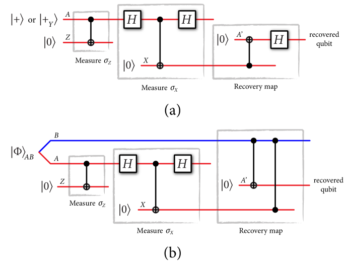
Figure 2: Circuits for experimental testing of our entropic uncertainty relation in (8). (a) Four different experimental tests in which one can prepare system $A$ as either $|+\rangle_{A}$ or $|+_{Y}\rangle_{A}$ and then perform either a $\sigma_{Z}$ Pauli measurement or not. Afterward, a $\sigma_{X}$ measurement is performed followed by the recovery operation from (20), whose aim it is to undo the effect of the $\sigma_{X}$ measurement. If $|+\rangle_{A}$ is prepared and $\sigma_{Z}$ is not measured, then it is possible to undo the effect of the $\sigma_{X}$ measurement and recover the qubit $|+\rangle$ perfectly in system $A^{\prime}$. If $|+\rangle_{A}$ is prepared and $\sigma_{Z}$ is then measured, it is possible to undo the effect of the $\sigma_{X}$ measurement with the same recovery operation. The same results hold if $|+_{Y}\rangle_{A}$ is prepared in system $A$ (i.e., the recovery operation undoes the effect of the $\sigma_{X}$ measurement). (b) Two different experimental tests in which one can prepare a maximally entangled Bell state $|\Phi\rangle_{AB}$ in systems $A$ and $B$, perform a Pauli $\sigma_{Z}$ measurement or not, perform a $\sigma_{X}$ measurement, followed by a recovery operation whose aim it is to undo the effect of the $\sigma_{X}$ measurement. In the case that $\sigma_{Z}$ is not measured, the recovery operation perfectly restores the maximally entangled state in systems $A^{\prime}$ and $B$. In the case that $\sigma_{Z}$ is measured, the recovery operation undoes the effect of the $\sigma_{X}$ measurement by restoring the maximally correlated state $(|00\rangle\langle 00|_{A^{\prime}B}+|11\rangle\langle 11|_{A^{\prime}B})/2$ in systems $A^{\prime}$ and $B$.

We have experimentally tested three of the examples from the previous section, namely, the $X$ eigenstate, the maximally entangled state, and the $Y$ eigenstate examples. We did so using the recently available IBM Quantum Experience (QE) IBM16 . Three experiments have already appeared on the arXiv, conducted remotely by theoretical groups testing out experiments which had never been performed previously AL16 ; D16 ; RTSE16 . The QE architecture consists of five fixed-frequency superconducting transmon qubits, laid out in a “star geometry” (four “corner” qubits and one in the center). It is possible to perform single-qubit gates $X$, $Y$, $Z$, $H$, $T$, $S$, and $S^{{\dagger}}$, a Pauli measurement $Z$, and Bloch sphere tomography on any single qubit. However, two-qubit operations are limited to controlled-NOT gates with any one of the corner qubits acting as the source and the center qubit as the target. Thus, one must “recompile” quantum circuits in order to meet these constraints. More information about the architecture is available at the user guide at IBM16 .

Our experiments realize and test three of the examples from the previous section and, in particular, are as follows:

1. Prepare system $A$ in the state $|+\rangle$. Measure Pauli $\sigma_{X}$ on qubit $A$ and place the outcome in register $X$. Perform the recovery channel given in (20), with output system $A^{\prime}$. Finally, perform Bloch sphere tomography on system $A^{\prime}$.

2. Prepare system $A$ in the state $|+\rangle$. Measure Pauli $\sigma_{Z}$ on qubit $A$ and place the outcome in register $Z$. Measure Pauli $\sigma_{X}$ on qubit $A$ and place the outcome in register $X$. Perform the recovery channel given in (20), with output system $A^{\prime}$. Finally, perform Bloch sphere tomography on system $A^{\prime}$.

3. Same as Experiment 1 but begin by preparing system $A$ in the state $|+_{Y}\rangle_{A}$.

4. Same as Experiment 2 but begin by preparing system $A$ in the state $|+_{Y}\rangle_{A}$.

5. Prepare systems $A$ and $B$ in the maximally entangled Bell state $|\Phi\rangle_{AB}$. Measure Pauli $\sigma_{X}$ on qubit $A$ and place the outcome in register $X$. Perform the recovery channel given in (28), with output systems $A^{\prime}$ and $B$. Finally, perform measurements of $\sigma_{X}$ on system $A^{\prime}$ and $\sigma_{X}$ on system $B$, or $\sigma_{Y}$ on system $A^{\prime}$ and $\sigma_{Y}^{\ast}$ on system $B$, or $\sigma_{Z}$ on system $A^{\prime}$ and $\sigma_{Z}$ on system $B$.

6. Prepare systems $A$ and $B$ in the maximally entangled Bell state $|\Phi\rangle_{AB}$. Measure Pauli $\sigma_{Z}$ on qubit $A$ and place the outcome in register $Z$. Measure Pauli $\sigma_{X}$ on qubit $A$ and place the outcome in register $X$. Perform the recovery channel given in (28), with output systems $A^{\prime}$ and $B$. Finally, perform measurements of $\sigma_{X}$ on system $A^{\prime}$ and $\sigma_{X}$ on system $B$, or $\sigma_{Y}$ on system $A^{\prime}$ and $\sigma_{Y}^{\ast}$ on system $B$, or $\sigma_{Z}$ on system $A^{\prime}$ and $\sigma_{Z}$ on system $B$.

A quantum circuit that can realize Experiments 1–4 is given in Figure 2(a), and a quantum circuit that can realize Experiments 5–6 is given in Figure 2(b). These circuits make use of standard quantum computing gates, detailed in book2000mikeandike , and one can readily verify that they ideally have the correct behavior, consistent with that discussed for the examples in the previous section. As stated above, it is necessary to recompile these circuits into a form which meets the constraints of the QE architecture.

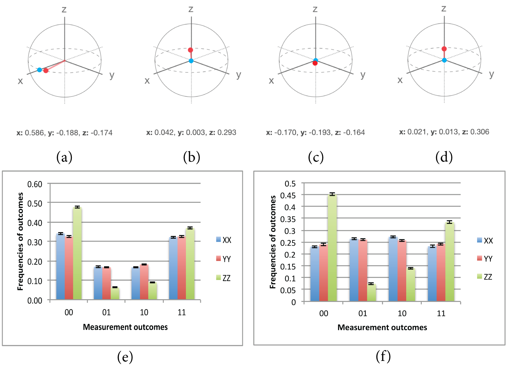
Figure 3: Results of experimental tests on the IBM QE quantum computer. Subfigures (a)–(f) correspond to Experiments 1–6 outlined in the main text, respectively. (a) The ideal state of the recovered qubit is $|+\rangle$, as predicted by (18) and depicted on the Bloch sphere as a blue dot. The figure plots the result of Bloch sphere tomography from the experimental tests (as a red dot). (b)–(d) The ideal state of the recovered qubit in each case is $\pi$ (the maximally mixed state), as predicted by (21), (31), and (32), respectively (again depicted as blue dots). The figure again plots the result of Bloch sphere tomography as red dots. (e) The ideal state of the recovered qubits is $|\Phi\rangle$ as predicted by (25). In such a case, measurement of the Pauli observables $\sigma_{i}$ on $A^{\prime}$ and $\sigma_{i}^{\ast}$ on $B$ for $i\in\{X,Y,Z\}$ should return 00 and 11 with probability 0.5 and 01 and 10 with probability zero. The plots reveal significant noise in the experiments, especially from the $\sigma_{X}$ and $\sigma_{Y}$ measurements. (f) The ideal state of the recovered qubits is the maximally correlated state $(|00\rangle\langle 00|+|11\rangle\langle 11|)/2$ as predicted in Section IV.1.3. In such a case, measurement of the Pauli observables $\sigma_{Z}$ on $A$ and $\sigma_{Z}$ on $B$ should return 00 and 11 with probability 0.5 and 01 and 10 with probability zero. Measurement of the Pauli observables $\sigma_{i}$ on $A$ and $\sigma_{i}^{\ast}$ on $B$ for $i\in\{X,Y\}$ should return all outcomes with equal probabilities. Again, the plots reveal significant noise in the experiments.

Figure 3 plots the results of Experiments 1–6. Each experiment consists of three measurements, with Experiments 1–4 having measurements of each of the Pauli operators, and Experiments 5–6 having three different measurements each as outlined above. Each of these is repeated 8192 times, for a total of $6\times 3\times 8192=147,456$ experiments. The standard error for each kind of experiment is thus $\sqrt{p_{c}(1-p_{c})/8192}$, where $p_{c}$ is the estimate of the probability of a given measurement outcome in a given experiment. The caption of Figure 3 features discussions of and comparisons between the predictions of the previous section and the experimental outcomes. While it is clear that the QE chip is subject to significant noise, there is still reasonable agreement with the theoretical predictions of the previous section. One observation we make regarding Figure 3(e) is that the frequencies for the outcomes of the $\sigma_{Z}$ and $\sigma_{Z}$ measurements are much closer to the theoretically predicted values than are the other measurement outcomes.

VI Conclusion

The entropic uncertainty relation with quantum side information is a unifying principle relating quantum uncertainty due to measurement incompatibility and entanglement. Here we refine and tighten this inequality with a state-dependent term related to how well one can reverse the action of a measurement. The tightening of the inequality is most pronounced when the measurements and state are all chosen from mutually unbiased bases, i.e., in our “maximum uncertainty” example with the measurements being $\sigma_{X}$ and $\sigma_{Z}$ and the initial state being a $\sigma_{Y}$ eigenstate. We have experimentally tested our theoretical predictions on the IBM Quantum Experience and find reasonable agreement between our predictions and experimental outcomes.

We note that in terms of the conditional min-entropy, other refinements of (6) are known DFW that look at the measurement channel and its own inverse channel, and it would be interesting to understand their relation. Going forward, it would furthermore be interesting to generalize the results established here to infinite-dimensional and multiple measurement scenarios.

Acknowledgments—The authors acknowledge discussions with Siddhartha Das, Michael Walter, and Andreas Winter. We are grateful to the team at IBM and the IBM Quantum Experience project. This work does not reflect the views or opinions of IBM or any of its employees. MB acknowledges funding provided by the Institute for Quantum Information and Matter, an NSF Physics Frontiers Center (NSF Grant PHY-1125565) with support of the Gordon and Betty Moore Foundation (GBMF-12500028). Additional funding support was provided by the ARO grant for Research on Quantum Algorithms at the IQIM (W911NF-12-1-0521). SW acknowledges support from STW, Netherlands and an NWO VIDI Grant. MMW is grateful to SW and her group for hospitality during a research visit to QuTech in May 2015 and acknowledges support from startup funds from the Department of Physics and Astronomy at LSU, the NSF under Award No. CCF-1350397, and the DARPA Quiness Program through US Army Research Office award W31P4Q-12-1-0019.

Appendix A Proof of (7) and (8)

The main idea of the proof of (7) follows the approach first put forward in CYZ11 (see also CCYZ12 ), for which the core argument is the non-increase of quantum relative entropy. Here we instead apply a refinement of this entropy inequality from Junge15 (see also W15 ; Sutter15 ; SBT16 ). In order to prove (7), we start by noting that it suffices to prove it when $\rho_{ABE}=|\psi\rangle\langle\psi|_{ABE}$ (i.e., the shared state is pure). This is because the conditional entropy only increases under the discarding of one part of the conditioning system. We consider the following isometric extensions of the measurement channels stinespring54 , which produce the measurement outcomes and post-measurement states:

$$U_{A\rightarrow XX^{\prime}A} \equiv\sum_{x}|x\rangle_{X}\otimes|x\rangle_{X^{\prime}}\otimes P_{A}^{x},$$ (34)

$$V_{A\rightarrow ZZ^{\prime}A} \equiv\sum_{z}|z\rangle_{Z}\otimes|z\rangle_{Z^{\prime}}\otimes Q_{A}^{z}.$$ (35)

We also define the following pure states, which represent purifications of the states $\sigma_{XBE}$ and $\omega_{ZBE}$ defined in (1) and (2), respectively:

$$|\sigma\rangle_{XX^{\prime}ABE} \equiv U_{A\rightarrow XX^{\prime}A}|\psi\rangle_{ABE},$$ (36)

$$|\omega\rangle_{ZZ^{\prime}ABE} \equiv V_{A\rightarrow ZZ^{\prime}A}|\psi\rangle_{ABE}.$$ (37)

Consider from duality of conditional entropy for pure states (see, e.g., CCYZ12 ) that

$$H(Z|E)_{\omega}=-H(Z|Z^{\prime}AB)_{\omega}=D(\omega_{ZZ^{\prime}AB}\|I_{Z}\otimes\omega_{Z^{\prime}AB}),$$ (38)

where $D(\rho\|\sigma)\equiv\operatorname{Tr}\{\rho[\log\rho-\log\sigma]\}$ is the quantum relative entropy U62 , defined as such when $\operatorname{supp}(\rho)\subseteq\operatorname{supp}(\sigma)$ and as $+\infty$ otherwise. Now consider the following quantum channel

$$\mathcal{P}_{ZZ^{\prime}A}(\cdot)\rightarrow\Pi(\cdot)\Pi+(I-\Pi)(\cdot)(I-\Pi),$$ (39)

where $\Pi\equiv VV^{{\dagger}}$. From the monotonicity of quantum relative entropy with respect to quantum channels Lindblad1975 ; U77 , we find that

$$D(\omega_{ZZ^{\prime}AB}\|I_{Z}\otimes\omega_{Z^{\prime}AB})\geq D(\mathcal{P}_{ZZ^{\prime}A}(\omega_{ZZ^{\prime}AB})\|\mathcal{P}_{ZZ^{\prime}A}(I_{Z}\otimes\omega_{Z^{\prime}AB})).$$ (40)

Consider that $\mathcal{P}_{ZZ^{\prime}A}(\omega_{ZZ^{\prime}AB})=\omega_{ZZ^{\prime}AB}$. Due to the fact that

$$(I-\Pi)\omega_{ZZ^{\prime}AB}(I-\Pi)=0,$$ (41)

and from the direct sum property of the quantum relative entropy (see, e.g., CCYZ12 ), we have that

$$D(\mathcal{P}_{ZZ^{\prime}A}(\omega_{ZZ^{\prime}AB})\|\mathcal{P}_{ZZ^{\prime}A}(I_{Z}\otimes\omega_{Z^{\prime}AB}))=D(\omega_{ZZ^{\prime}AB}\|\Pi(I_{Z}\otimes\omega_{Z^{\prime}AB})\Pi).$$ (42)

Consider that

$$\Pi(I_{Z}\otimes\omega_{Z^{\prime}AB})\Pi=VV^{{\dagger}}(I_{Z}\otimes\omega_{Z^{\prime}AB})VV^{{\dagger}}=V\!\left(\sum_{z}Q_{A}^{z}\rho_{AB}Q_{A}^{z}\right)V^{{\dagger}}.$$ (43)

This, combined with $\omega_{ZZ^{\prime}AB}=V\rho_{AB}V^{{\dagger}}$, then implies that

$$D(\omega_{ZZ^{\prime}AB}\|\Pi(I_{Z}\otimes\omega_{Z^{\prime}AB})\Pi) =D\!\left(V\rho_{AB}V^{{\dagger}}\middle\|V\!\left(\sum_{z}Q_{A}^{z}\rho_{AB}Q_{A}^{z}\right)V^{{\dagger}}\right)$$ (44)

$$=D\!\left(\rho_{AB}\middle\|\sum_{z}Q_{A}^{z}\rho_{AB}Q_{A}^{z}\right),$$ (45)

where the last equality follows from the invariance of quantum relative entropy with respect to isometries. Now consider the following quantum channel:

$$\mathcal{M}_{A\rightarrow X}\equiv\operatorname{Tr}_{X^{\prime}A}\circ\ \mathcal{U}_{A\rightarrow XX^{\prime}A},$$ (46)

where $\mathcal{U}_{A\rightarrow XX^{\prime}A}(\cdot)\equiv U(\cdot)U^{{\dagger}}$. Consider that $\mathcal{M}_{A\rightarrow X}(\rho_{AB})=\sigma_{XB}$. Also, we can calculate

$$\mathcal{M}_{A\rightarrow X}\!\left(\sum_{z}Q_{A}^{z}\rho_{AB}Q_{A}^{z}\right)$$ (47)

as follows:

$$(\operatorname{Tr}_{X^{\prime}A}\circ\mathcal{U}_{A\rightarrow XX^{\prime}A})\left(\sum_{z}Q_{A}^{z}\rho_{AB}Q_{A}^{z}\right)=\theta_{XB}.$$ (48)

From Junge15 , we have the following inequality holding for a density operator $\rho$, a positive semi-definite operator $\sigma$, and a quantum channel $\mathcal{N}$:

$$D(\rho\|\sigma)-D(\mathcal{N}(\rho)\|\mathcal{N}(\sigma))\geq-\log F(\rho,\mathcal{R}(\mathcal{N}(\rho))),$$ (49)

where $\operatorname{supp}(\rho)\subseteq\operatorname{supp}(\sigma)$ and $\mathcal{R}$ is a recovery channel with the property that $\mathcal{R}(\mathcal{N}(\sigma))=\sigma$. Specifically, $\mathcal{R}$ is what is known as a variant of the Petz recovery channel, having the form

$$\mathcal{R}(\cdot)\equiv \int\mathrm{d}t\,p(t)\,\sigma^{-it/2}\mathcal{R}_{\sigma,\mathcal{N}}(\mathcal{N}(\sigma)^{it/2}(\cdot)\mathcal{N}(\sigma)^{-it/2})\sigma^{it/2}$$

$$\mathrm{with}\quad p(t)\equiv\frac{\pi}{2}(\cosh(\pi t)+1)^{-1},$$ (50)

where $\mathcal{R}_{\sigma,\mathcal{N}}$ is the Petz recovery channel Petz1986 ; Petz1988 ; HJPW04  defined as

$$\mathcal{R}_{\sigma,\mathcal{N}}(\cdot)\equiv\sigma^{1/2}\mathcal{N}^{{\dagger}}\!\left(\mathcal{N}(\sigma)^{-1/2}(\cdot)\mathcal{N}(\sigma)^{-1/2}\right)\sigma^{1/2},$$ (51)

with $\mathcal{N}^{{\dagger}}$ the adjoint of $\mathcal{N}$ (with respect to the Hilbert–Schmidt inner product). Applying this to our case, we find that

$$D\!\left(\rho_{AB}\middle\|\sum_{z}Q_{A}^{z}\rho_{AB}Q_{A}^{z}\right)\geq D\!\left(\mathcal{M}_{A\rightarrow X}(\rho_{AB})\middle\|\mathcal{M}_{A\rightarrow X}\!\left(\sum_{z}Q_{A}^{z}\rho_{AB}Q_{A}^{z}\right)\right)\\ -\log F(\rho_{AB},\mathcal{R}_{XB\to AB}(\mathcal{M}_{A\rightarrow X}(\rho_{AB}))),$$ (52)

where the recovery channel is such that

$$\mathcal{R}_{XB\to AB}\!\left(\mathcal{M}_{A\rightarrow X}\!\left(\sum_{z}Q_{A}^{z}\rho_{AB}Q_{A}^{z}\right)\right)=\sum_{z}Q_{A}^{z}\rho_{AB}Q_{A}^{z}.$$ (53)

Consider from our development above that

$$D\!\left(\mathcal{M}_{A\rightarrow X}(\rho_{AB})\middle\|\mathcal{M}_{A\rightarrow X}\!\left(\sum_{z}Q_{A}^{z}\rho_{AB}Q_{A}^{z}\right)\right) =D(\sigma_{XB}\|\theta_{XB})$$ (54)

$$\geq D(\sigma_{XB}\|I_{X}\otimes\sigma_{B})-\log c,$$ (55)

where we have used $\sigma\leq\sigma^{\prime}\Rightarrow D(\rho\|\sigma^{\prime})\leq D(\rho\|\sigma)$ (see, e.g., CCYZ12 ), applied to $Q_{A}^{z}P_{A}^{x}Q_{A}^{z}=|Q_{A}^{z}P_{A}^{x}|^{2}\leq c\cdot I_{A}$, with $c$ defined in (5). Putting everything together, we conclude that

$$D(\omega_{ZZ^{\prime}AB}\|I_{Z}\otimes\omega_{Z^{\prime}AB})\geq D(\sigma_{XB}\|I_{X}\otimes\sigma_{B})-\log c-\log F(\rho_{AB},\mathcal{R}_{XB\to AB}(\sigma_{XB})),$$ (56)

which, after a rewriting, is equivalent to (7) coupled with the constraint in (53).

The inequality in (8) follows from (7) by letting $|\psi\rangle_{ABE}$ be a purification of $\rho_{AB}$ and observing that

$$H(Z|E)_{\omega}-H(Z|B)_{\omega}=-H(A|B)_{\rho},$$ (57)

whenever $\rho_{ABE}$ is a pure state and $Q_{A}^{z}=|z\rangle\langle z|_{A}$ for some orthonormal basis $\{|z\rangle_{A}\}_{z}$.

Appendix B Explicit form of recovery map

Here we establish the explicit form given in (10) for the recovery map, in the case that $\{Q_{A}^{z}=|z\rangle\langle z|_{A}\}$ for some orthonormal basis $\{|z\rangle_{A}\}_{z}$. The main idea is to determine what $\mathcal{R}_{XB\to AB}$ in (52) should be by inspecting (49) and (50). For our setup, we are considering a bipartite state $\rho_{AB}$, a set $\{Q_{A}^{z}\}$ of measurement operators, and the measurement channel

$$\mathcal{M}_{A\rightarrow X}(\zeta_{A})\equiv\sum_{x}\operatorname{Tr}\{P_{A}^{x}\zeta_{A}\}|x\rangle\langle x|_{X},$$ (58)

where $\{P_{A}^{x}\}_{x}$ is a set of projective measurement operators. The entropy inequality in (52) reduces to

$$D\!\left(\rho_{AB}\middle\|\sum_{z}|z\rangle\langle z|_{A}\otimes\omega_{B}^{z}\right)-D\!\left(\mathcal{M}_{A\rightarrow X}(\rho_{AB})\middle\|\sum_{x}|x\rangle\langle x|_{X}\otimes\theta_{B}^{x}\right)\\ \geq-\log F(\rho_{AB},\mathcal{R}_{XB\rightarrow AB}(\mathcal{M}_{A\rightarrow X}(\rho_{AB}))),$$ (59)

where

$$\omega_{B}^{z}\equiv(\langle z|_{A}\otimes I_{B})\rho_{AB}(|z\rangle_{A}\otimes I_{B}),\qquad\theta_{B}^{x}\equiv\sum_{z}\langle z|_{A}P_{A}^{x}|z\rangle_{A}\omega_{B}^{z}.$$ (60)

Observe that

$$\sum_{x}|x\rangle\langle x|_{X}\otimes\theta_{B}^{x}=\mathcal{M}_{A\rightarrow X}\!\left(\sum_{z}|z\rangle\langle z|_{A}\otimes\omega_{B}^{z}\right).$$ (61)

Writing the measurement channel as

$$\mathcal{M}_{A\rightarrow X}(\zeta_{A}) \equiv\sum_{x}\operatorname{Tr}\{P_{A}^{x}\zeta_{A}P_{A}^{x}\}|x\rangle\langle x|_{X}=\sum_{x,j}\langle j|_{A}P_{A}^{x}\zeta_{A}P_{A}^{x}|j\rangle_{A}|x\rangle\langle x|_{X}$$ (62)

$$=\sum_{x,j}|x\rangle_{X}\langle j|_{A}P_{A}^{x}\zeta_{A}P_{A}^{x}|j\rangle_{A}\langle x|_{X},$$ (63)

we can see that a set of Kraus operators for it is $\{|x\rangle_{X}\langle j|_{A}P_{A}^{x}\}_{x,j}$. So its adjoint is as follows:

$$\left(\mathcal{M}_{A\rightarrow X}\right)^{{\dagger}}(\kappa_{X}) =\sum_{x,j}P_{A}^{x}|j\rangle_{A}\langle x|_{X}\kappa_{X}|x\rangle_{X}\langle j|_{A}P_{A}^{x}=\sum_{x,j}\langle x|_{X}\kappa_{X}|x\rangle_{X}P_{A}^{x}|j\rangle_{A}\langle j|_{A}P_{A}^{x}$$ (64)

$$=\sum_{x}\langle x|_{X}\kappa_{X}|x\rangle_{X}P_{A}^{x}.$$ (65)

So by inspecting (49) and (50), we see that the recovery map has the following form:

$$\mathcal{R}_{XB\rightarrow AB}(\xi_{XB})$$

$$=\int dt\ p(t)\ \left(\sum_{z}|z\rangle\langle z|_{A}\otimes\omega_{B}^{z}\right)^{\frac{1-it}{2}}\sum_{x}P_{A}^{x}\left(\langle x|_{X}\otimes I_{B}\right)\left(\sum_{x^{\prime}}|x^{\prime}\rangle\langle x^{\prime}|_{X}\otimes\theta_{B}^{x^{\prime}}\right)^{\frac{-1+it}{2}}(\xi_{XB})$$

$$\qquad\qquad\left(\sum_{x^{\prime\prime}}|x^{\prime\prime}\rangle\langle x^{\prime\prime}|_{X}\otimes\theta_{B}^{x^{\prime\prime}}\right)^{\frac{-1-it}{2}}\left(|x\rangle_{X}\otimes I_{B}\right)\left(\sum_{z^{\prime}}|z^{\prime}\rangle\langle z^{\prime}|_{A}\otimes\omega_{B}^{z^{\prime}}\right)^{\frac{1+it}{2}}$$ (66)

$$=\int dt\ p(t)\ \left(\sum_{z}|z\rangle\langle z|_{A}\otimes\left(\omega_{B}^{z}\right)^{\frac{1-it}{2}}\right)\sum_{x}P_{A}^{x}\left(\langle x|_{X}\otimes I_{B}\right)$$

$$\qquad\qquad\left[\left(\sum_{x^{\prime}}|x^{\prime}\rangle\langle x^{\prime}|_{X}\otimes\left(\theta_{B}^{x^{\prime}}\right)^{\frac{-1+it}{2}}\right)(\xi_{XB})\left(\sum_{x^{\prime\prime}}|x^{\prime\prime}\rangle\langle x^{\prime\prime}|_{X}\otimes\left(\theta_{B}^{x^{\prime\prime}}\right)^{\frac{-1-it}{2}}\right)\right]$$

$$\qquad\qquad\left(|x\rangle_{X}\otimes I_{B}\right)\left(\sum_{z^{\prime}}|z^{\prime}\rangle\langle z^{\prime}|_{A}\otimes\left(\omega_{B}^{z^{\prime}}\right)^{\frac{1+it}{2}}\right)$$ (67)

$$=\int dt\ p(t)\ \left(\sum_{z}|z\rangle\langle z|_{A}\otimes\left(\omega_{B}^{z}\right)^{\frac{1-it}{2}}\right)\sum_{x,x^{\prime},x^{\prime\prime}}P_{A}^{x}\langle x|_{X}|x^{\prime}\rangle\langle x^{\prime}|_{X}\otimes\left(\theta_{B}^{x^{\prime}}\right)^{\frac{-1+it}{2}}(\xi_{XB})$$

$$\qquad\qquad|x^{\prime\prime}\rangle\langle x^{\prime\prime}|_{X}|x\rangle_{X}\otimes\left(\theta_{B}^{x^{\prime\prime}}\right)^{\frac{-1-it}{2}}\left(\sum_{z^{\prime}}|z^{\prime}\rangle\langle z^{\prime}|_{A}\otimes\left(\omega_{B}^{z^{\prime}}\right)^{\frac{1+it}{2}}\right)$$ (68)

$$=\int dt\ p(t)\ \left(\sum_{z}|z\rangle\langle z|_{A}\otimes\left(\omega_{B}^{z}\right)^{\frac{1-it}{2}}\right)\sum_{x}P_{A}^{x}\langle x|_{X}\otimes\left(\theta_{B}^{x}\right)^{\frac{-1+it}{2}}(\xi_{XB})|x\rangle_{X}\otimes\left(\theta_{B}^{x}\right)^{\frac{-1-it}{2}}$$

$$\qquad\qquad\left(\sum_{z^{\prime}}|z^{\prime}\rangle\langle z^{\prime}|_{A}\otimes\left(\omega_{B}^{z^{\prime}}\right)^{\frac{1+it}{2}}\right)$$ (69)

$$=\int dt\ p(t)\ \sum_{z,x,z^{\prime}}|z\rangle\langle z|_{A}P_{A}^{x}|z^{\prime}\rangle\langle z^{\prime}|_{A}\otimes\left(\omega_{B}^{z}\right)^{\frac{1-it}{2}}\left(\theta_{B}^{x}\right)^{\frac{-1+it}{2}}\operatorname{Tr}_{X}\{|x\rangle\langle x|_{X}(\xi_{XB})\}\left(\theta_{B}^{x}\right)^{\frac{-1-it}{2}}\left(\omega_{B}^{z^{\prime}}\right)^{\frac{1+it}{2}}.$$ (70)

We can thus abbreviate its action as

$$\mathcal{R}_{XB\rightarrow AB}(\xi_{XB})=\ \sum_{z,x,z^{\prime}}|z\rangle\langle z|_{A}P_{A}^{x}|z^{\prime}\rangle\langle z^{\prime}|_{A}\otimes\mathcal{R}_{XB\rightarrow B}^{x,z,z^{\prime}}(\xi_{XB}),$$ (71)

where

$$\mathcal{R}_{XB\rightarrow B}^{x,z,z^{\prime}}(\xi_{XB})\equiv\int dt\ p(t)\left(\omega_{B}^{z}\right)^{\frac{1-it}{2}}\left(\theta_{B}^{x}\right)^{\frac{-1+it}{2}}\operatorname{Tr}_{X}\{|x\rangle\langle x|_{X}(\xi_{XB})\}\left(\theta_{B}^{x}\right)^{\frac{-1-it}{2}}\left(\omega_{B}^{z^{\prime}}\right)^{\frac{1+it}{2}}.$$ (72)

(Note that $\mathcal{R}_{XB\rightarrow B}^{x,z,z^{\prime}}$ is not a channel.) So then the action on the classical–quantum state $\sigma_{XB}$, defined as

$$\sigma_{XB}\equiv\sum_{x}|x\rangle\langle x|_{X}\otimes\sigma_{B}^{x},$$ (73)

with $\sigma_{B}^{x}\equiv\operatorname{Tr}_{A}\{P_{A}^{x}\rho_{AB}\}$, is as follows:

$$\mathcal{R}_{XB\rightarrow AB}(\sigma_{XB})=\sum_{z,x,z^{\prime}}|z\rangle\langle z|_{A}P_{A}^{x}|z^{\prime}\rangle\langle z^{\prime}|_{A}\otimes\int dt\ p(t)\left(\omega_{B}^{z}\right)^{\frac{1-it}{2}}\left(\theta_{B}^{x}\right)^{\frac{-1+it}{2}}\sigma_{B}^{x}\left(\theta_{B}^{x}\right)^{\frac{-1-it}{2}}(\omega_{B}^{z^{\prime}})^{\frac{1+it}{2}}.$$ (74)

References

• [1] Werner Heisenberg. Über den anschaulichen inhalt der quantentheoretischen kinematik und mechanik. Zeitschrift für Physik, 43:172–198, 1927.
• [2] Mario Berta, Matthias Christandl, Roger Colbeck, Joseph M. Renes, and Renato Renner. The uncertainty principle in the presence of quantum memory. Nature Physics, 6:659–662, September 2010. arXiv:0909.0950.
• [3] Howard P. Robertson. The uncertainty principle. Physical Review, 34(1):163, July 1929.
• [4] Isidore I. Hirschman. A note on entropy. American Journal of Mathematics, 79(1):152–156, January 1957.
• [5] Iwo Bialynicki-Birula and Jerzy Mycielski. Uncertainty relations for information entropy in wave mechanics. Communications in Mathematical Physics, 44(2):129–132, June 1975.
• [6] William Beckner. Inequalities in Fourier analysis. Annals of Mathematics, 102(1):159, July 1975.
• [7] David Deutsch. Uncertainty in quantum measurements. Physical Review Letters, 50(9):631–633, February 1983.
• [8] Karl Kraus. Complementary observables and uncertainty relations. Physical Review D, 35(10):3070–3075, May 1987.
• [9] Hans Maassen and J. B. M. Uffink. Generalized entropic uncertainty relations. Physical Review Letters, 60(12):1103–1106, March 1988.
• [10] M. Krishna and K. R. Parthasarathy. An entropic uncertainty principle for quantum measurements. Sankhya: The Indian Journal of Statistics, Series A, 64(3):842–851, October 2002.
• [11] Matthias Christandl and Andreas Winter. Uncertainty, monogamy, and locking of quantum correlations. IEEE Transactions on Information Theory, 51(9):3159–3165, September 2005. arXiv:quant-ph/0501090.
• [12] Joseph M. Renes and Jean-Christian Boileau. Conjectured strong complementary information tradeoff. Physical Review Letters, 103(2):020402, July 2009. arXiv:0806.3984.
• [13] Mark A. Naimark. Spectral functions of a symmetric operator. Izv. Acad. nauk SSSR Ser. Mat., 4:277–318, 1940.
• [14] Marco Tomamichel, Serge Fehr, Jedrzej Kaniewski, and Stephanie Wehner. A monogamy-of-entanglement game with applications to device-independent quantum cryptography. New Journal of Physics, 15(10):103002, October 2013. arXiv:1210.4359.
• [15] Marco Tomamichel and Renato Renner. Uncertainty relation for smooth entropies. Physical Review Letters, 106(11):110506, March 2011. arXiv:1009.2015.
• [16] Marco Tomamichel, Charles Ci Wen Lim, Nicolas Gisin, and Renato Renner. Tight finite-key analysis for quantum cryptography. Nature Communications, 3:634, January 2012. arXiv:1103.4130.
• [17] Marco Tomamichel and Anthony Leverrier. A rigorous and complete proof of finite key security of quantum key distribution. June 2015. arXiv:1506.08458.
• [18] Patrick J. Coles, Li Yu, and Michael Zwolak. Relative entropy derivation of the uncertainty principle with quantum side information. December 2011. arXiv:1105.4865.
• [19] Rupert L. Frank and Elliott H. Lieb. Extended quantum conditional entropy and quantum uncertainty inequalities. Communications in Mathematical Physics, 323(2):487–495, October 2013. arXiv:1204.0825.
• [20] Fabian Furrer, Mario Berta, Marco Tomamichel, Volkher B. Scholz, and Matthias Christandl. Position-momentum uncertainty relations in the presence of quantum memory. Journal of Mathematical Physics, 55(12):122205, August 2014. arXiv:1308.4527.
• [21] Marius Junge, Renato Renner, David Sutter, Mark M. Wilde, and Andreas Winter. Universal recovery from a decrease of quantum relative entropy. September 2015. arXiv:1509.07127.
• [22] Mark M. Wilde. Recoverability in quantum information theory. Proceedings of the Royal Society of London A: Mathematical, Physical and Engineering Sciences,, 471(2182):20150338, October 2015. arXiv:1505.04661.
• [23] David Sutter, Marco Tomamichel, and Aram W. Harrow. Strengthened monotonicity of relative entropy via pinched Petz recovery map. IEEE Transactions on Information Theory, 62(5):2907–2913, May 2016. arXiv:1507.00303.
• [24] David Sutter, Mario Berta, and Marco Tomamichel. Multivariate trace inequalities. April 2016. arXiv:1604.03023.
• [25] Göran Lindblad. Completely positive maps and entropy inequalities. Communications in Mathematical Physics, 40(2):147–151, June 1975.
• [26] Armin Uhlmann. Relative entropy and the Wigner-Yanase-Dyson-Lieb concavity in an interpolation theory. Communications in Mathematical Physics, 54(1):21–32, 1977.
• [27] Mark M. Wilde. Quantum Information Theory. Cambridge University Press, 2013. arXiv:1106.1445.
• [28] Takahiro Sagawa. Lectures on Quantum Computing, Thermodynamics and Statistical Physics, chapter Second Law-Like Inequalities with Quantum Relative Entropy: An Introduction, page 127. World Scientific, 2012. arXiv:1202.0983.
• [29] Armin Uhlmann. The “transition probability” in the state space of a *-algebra. Reports on Mathematical Physics, 9(2):273–279, 1976.
• [30] Patrick J. Coles, Roger Colbeck, Li Yu, and Michael Zwolak. Uncertainty relations from simple entropic properties. Physical Review Letters, 108(21):210405, May 2012. arXiv:1112.0543.
• [31] IBM. The quantum experience. URL http://www.research.ibm.com/quantum/.
• [32] Daniel Alsina and José Ignacio Latorre. Experimental test of Mermin inequalities on a 5-qubit quantum computer. May 2016. arXiv:1605.04220.
• [33] Simon J. Devitt. Performing quantum computing experiments in the cloud. May 2016. arXiv:1605.05709.
• [34] R.P. Rundle, Todd Tilma, J. H. Samson, and M. J. Everitt. Quantum state reconstruction made easy: a direct method for tomography. May 2016. arXiv:1605.08922.
• [35] Michael A. Nielsen and Isaac L. Chuang. Quantum Computation and Quantum Information. Cambridge University Press, 2000.
• [36] Frederic Dupuis, Omar Fawzi, and Stephanie Wehner. Entanglement sampling and its applications. IEEE Transactions on Information Theory, 61(2):1093–1112, February 2015. arXiv:1305.1316.
• [37] W. Forrest Stinespring. Positive Functions On C*-Algebras. Proceedings of the American Mathematical Society, 6:211–216, 1955.
• [38] Hisaharu Umegaki. Conditional expectations in an operator algebra IV (entropy and information). Kodai Mathematical Seminar Reports, 14(2):59–85, 1962.
• [39] Dénes Petz. Sufficient subalgebras and the relative entropy of states of a von Neumann algebra. Communications in Mathematical Physics, 105(1):123–131, March 1986.
• [40] Dénes Petz. Sufficiency of channels over von Neumann algebras. Quarterly Journal of Mathematics, 39(1):97–108, 1988.
• [41] Patrick Hayden, Richard Jozsa, Denes Petz, and Andreas Winter. Structure of states which satisfy strong subadditivity of quantum entropy with equality. Communications in Mathematical Physics, 246(2):359–374, April 2004. arXiv:quant-ph/0304007.