Error analysis for POD Approximations of
infinite horizon problems via the
Dynamic Programming approach

Abstract

In this paper infinite horizon optimal control problems for nonlinear high-dimensional dynamical systems are studied. Nonlinear feedback laws can be computed via the value function characterized as the unique viscosity solution to the corresponding Hamilton-Jacobi-Bellman (HJB) equation which stems from the dynamic programming approach. However, the bottleneck is mainly due to the curse of dimensionality and HJB equations are only solvable in a relatively small dimension. Therefore, a reduced-order model is derived for the dynamical system and for this purpose the method of proper orthogonal decomposition (POD) is used. The resulting errors in the HJB equations are estimated by an a-priori error analysis, which suggests a new sampling strategy for the POD method. Numerical experiments illustrates the theoretical findings.

1 Introduction

The Dynamic Programming approach to the solution of optimal control problems driven by dynamical systems in $\mathbb{R}^{n}$ offers a nice framework for the approximation of feedback laws and optimal trajectories. It suffers from the bottleneck of the computation of the value function since this requires the approximation of a nonlinear partial differential equation in dimension $n$. This is a very challenging problem in high dimension due to the huge amount of memory allocations necessary to work on a grid and to the low regularity properties of the value function (which is typically only Lipschitz continuous even for regular dynamics and running costs). Despite the number of theoretical results established for many classical control problems via the dynamic programming approach (see e.g. the monographies by Bardi and Capuzzo-Dolcetta [8] on deterministic control problems and by Fleming and Soner [19] on stochastic control problems) this has always been the main obstacle to apply this nowadays rather complete theory to real applications. The ”curse of dimensionality” has been mitigated via domain decomposition techniques and the development of rather efficient numerical methods but it is still a big obstacle. Although a detailed description of these contributions goes beyond the scopes of this paper, we want to mention [18] for a domain decomposition method with overlapping between the subdomains and [11] for similar results without overlapping. It is important to note that in these papers the method is applied to subdomains with a rather simple geometry (see the book by Quarteroni and Valli [32] for a general introduction to this technique) in order to apply transmission conditions at the boundaries. More recently another way to decompose the problem has been proposed by Krener and Navasca [31] who have used a patchy decomposition based on Al’brekht method. Later in the paper [10] the patchy idea has been implemented taking into account an approximation of the underlying optimal dynamics to obtain subdomains which are almost invariant with respect to the optimal dynamics, clearly in this case the geometry of the subdomains can be rather complex but the transmission conditions at the internal boundaries can be eliminated saving on the overall complexity of the algorithm. In general, domain decomposition methods reduce a huge problem into subproblems of manageable size and allows to mitigate the storage limitation distributing the computation over several processors. However, the approximation schemes used in every subdomain are rather standard. Another improvement can be obtained using efficient acceleration methods for the computation of the value function in every subdomain. To this end one can use Fast Marching methods [34, 35] and Fast Sweeping methods [37] for specific classes of Hamilton-Jacobi equations. In the framework of optimal control problems an efficient acceleration technique based on the coupling between value and policy iterations has been recently proposed and studied by Alla, Falcone and Kalise in [3, 4]. Finally, we should mention that the interested reader can find in [17] a number of successful applications to optimal control problems and games in rather low dimension.

In parallel to these results several model reduction techniques have been developed to deal with high dimensional dynamics in a rather economic way. These techniques are really necessary when dealing with optimal control problems governed by partial differential equations. Despite the vast literature concerning the analysis and numerical approximation of optimal control problems for PDEs, the amount of works devoted to the synthesis of feedback controllers is rather small. In this direction, the application of the dynamic programming principle (DPP) is a powerful technique which has been applied mainly to linear dynamics, quadratic cost functions and unbounded control space, the so-called linear quadratic regulator (LQR) control problem. For this problem an explicit feedback controller can be computed by means of the solution of an algebraic Riccati equation. However if the underlying structural assumptions are removed, the feedback control has to be obtained via the approximation of a Hamilton-Jacobi-Bellman equation defined over the state space of the system dynamics. As we mentioned, this is a major bottleneck for the application of DPP-based techniques in the optimal control of PDEs, as the natural approach for this class of control problems is to consider a semi-discretization (in space) via finite elements or finite differences of the abstract governing equations, leading to an inherently high-dimensional state space. However, in the last years several steps have been made to obtain reduced-order models for complicated dynamics and by the application of these techniques it is now possible to have a reasonable approximation of large-scale dynamics using a rather small number of basis functions. This can open the way to the DPP approach in high-dimensional systems.

Reduced-order models are used in PDE-constrained optimization in various ways; see, e.g., [21, 24, 33] for a survey. However, the main stream for the optimal control of PDEs is still related to open-loop controls based on the Pontryagin Maximum Principle (an extensive presentation of this classical approach can be found in the monograph [23, 38]). Let us refer to [5, 7, 27, 28, 29], where it has been observed that models of reduced order can play an important and very useful role in the implementation of feedback laws. More recently, the Proper Orthogonal Decomposition (POD) has been proposed for PDE control problems in order to reduce the dynamics to a small number of state variable via a careful selection of the snapshots. This technique, coupled with the Dynamic Programming approach, has been developed mainly for linear equations starting from the heat equation where one can take advantage of the regularity of the solutions to reduce the dimension [7] and then attacking more difficult problems as the advection-diffusion equation [1, 2, 6, 25], Burgers’s equation [27, 28] and Navier-Stokes [5].

The aim of this paper is to study the interplay between reduced-order dynamics, the associated dynamic programming equation, the resulting feedback controller and its performance over the high-dimensional system. In our analysis we will derive some a-priori error estimates which take into account the time and space discretization parameter $\Delta t$ and $\Delta x$ as well as the dimension $\ell$ of the POD basis functions used for the reduced model.

The paper is organized as follows: in Section 2 we recall some basic facts about the approximation of the infinite horizon problem via the dynamic programming approach. Section 3 is devoted to present in short the POD technique and the basic ideas behind the construction of the reduced model. In Section 4 we present the main results and our a-priori estimates for the numerical approximation of the reduced model. These a-priori estimates have been also used in the construction of the algorithm which is described in detail in Section 5. Some numerical tests are presented and analyzed in Section 6 and finally we draw some conclusions in Section 7.

2 Optimal control problem

In this section we will recall the Dynamic Programming approach and its numerical approximation for the solution of infinite horizon control problem.

2.1 The infinite horizon problem

For given nonlinear mapping $f:\mathbb{R}^{n}\times\mathbb{R}^{m}\to\mathbb{R}^{n}$ and initial condition $y_{\circ}\in\mathbb{R}^{n}$ let us consider the following controlled nonlinear dynamical systems

(2.1) $$\dot{y}(t)=f\big{(}y(t),u(t)\big{)}\in\mathbb{R}^{n}\text{ for }t>0,\quad y(0)=y_{\circ}\in\mathbb{R}^{n}$$

together with the infinite horizon cost functional

(2.2) $$J(y,u)=\int_{0}^{\infty}g\big{(}y(t),u(t)\big{)}e^{-\lambda t}\,\mathrm{d}t$$

In (2.2) we assume that $\lambda>0$ is a given weighting parameter and $g$ maps $\mathbb{R}^{n}\times\mathbb{R}^{m}$ to $\mathbb{R}$. We call $y$ the state and $u$ the control. The set of admissible controls has the form

$${\mathbb{U}_{\mathsf{ad}}}=\big{\{}u\in\mathbb{U}\,\big{|}\,u(t)\in{U_{\mathsf{ad}}}\text{ for almost all }t\geq 0\big{\}},$$

where we set $\mathbb{U}=L^{2}(0,\infty;\mathbb{R}^{m})$ and ${U_{\mathsf{ad}}}\subset\mathbb{R}^{m}$ denotes a compact, convex subset.

Let $\mathrm{M}\in\mathbb{R}^{n\times n}$ denote a symmetric, positive definite (mass) matrix with smallest and largest positive eigenvalues $\lambda_{min}$ and $\lambda_{max}$, respectively. Then, we introduce the following weighted inner product in $\mathbb{R}^{n}$:

$${\langle y,\tilde{y}\rangle}_{\mathrm{M}}=y^{\top}\mathrm{M}\tilde{y}\quad\text{for }y,\tilde{y}\in\mathbb{R}^{n},$$

where ‘$\top$’ stands for the transpose of a given vector or matrix. By $\|\cdot\|_{\mathrm{M}}=\langle\cdot\,,\cdot\rangle_{\mathrm{M}}^{1/2}$ we define the associated induced norm. Recall that we have

$$\lambda_{min}\,{\|y\|}_{2}^{2}\leq{\|y\|}_{\mathrm{M}}^{2}\leq\lambda_{max}\,{\|y\|}_{2}^{2}\quad\text{for all }y\in\mathbb{R}^{n}.$$

Then, $y$ solves (2.1) if

(2.3) $${\langle\dot{y}(t)-f(y(t),u(t)),\varphi\rangle}_{\mathrm{M}} =0 \text{for all }\varphi\in\mathbb{R}^{n}\text{ and for almost all }t>0,$$

$${\langle y(0)-y_{\circ},\varphi\rangle}_{\mathrm{M}} =0 \text{for all }\varphi\in\mathbb{R}^{n}$$

We call (2.3) the variational formulation of the dynamical system. Let us suppose that (2.1) has a unique solution $y=y(u;y_{\circ})\in\mathbb{Y}=H^{1}(0,\infty;\mathbb{R}^{n})$ for every admissible control $u\in{\mathbb{U}_{\mathsf{ad}}}$ and for every initial condition $y_{\circ}\in\mathbb{R}^{n}$; see, e.g., [8, Chapter III]. Thus, we can define the reduced cost functional as follows:

$$\widehat{J}(u;y_{\circ})=J(y(u;y_{\circ}),u)\quad\text{for }u\in{\mathbb{U}_{\mathsf{ad}}}\text{ and }y_{\circ}\in\mathbb{R}^{n},$$

where $y(u;y_{\circ})$ solves (2.1) for given control $u$ and initial condition $y_{\circ}$. Then, our optimal control can be formulated as follows: for given $y_{\circ}\in\mathbb{R}^{n}$ we consider

($$\mathbf{\widehat{P}} \min_{u\in{\mathbb{U}_{\mathsf{ad}}}}\widehat{J}(u;y_{\circ}).$$)

2.2 The Hamilton-Jacobi-Bellman equation and its time discretization

We define the value function of the problem $v:\mathbb{R}^{n}\to\mathbb{R}$ as follows:

$$v(y)=\inf\big{\{}\widehat{J}(u;y)\,\big{|}\,u\in{\mathbb{U}_{\mathsf{ad}}}\big{\}}\quad\text{for }y\in\mathbb{R}^{n}.$$

This function gives the best value for every initial condition, given the set of admissible controls ${U_{\mathsf{ad}}}$. It is characterized as the unique viscosity solution of the Hamilton-Jacobi-Bellman (HJB) equation corresponding the infinite horizon

(2.4) $$\lambda v(y)+\sup_{u\in{U_{\mathsf{ad}}}}\big{\{}-f(y,u)\cdot\nabla v(y)-g(y,u)\big{\}}=0\quad\text{for }y\in\mathbb{R}^{n}.$$

In order to construct the approximation scheme (as in [15]) let us consider first a time discretization where $h$ is a strictly positive step size. A dynamic programming principle for the discrete time problem holds true giving the following semi-discrete scheme for (2.4)

(2.5) $$v_{h}(y)=\min_{u\in{U_{\mathsf{ad}}}}\big{\{}(1-\lambda h)v_{h}(y+hf(y,u))+hg(y,u)\big{\}}\quad\text{for }y\in\mathbb{R}^{n}.$$

Throughout our paper we suppose the following hypotheses.

Assumption 1.

1. The right-hand side $f:\mathbb{R}^{n}\times\mathbb{R}^{m}\to\mathbb{R}^{n}$ is continuous and globally Lipschitz-continuous in the first argument, i.e., there exists an $L_{f}>0$ satisfying

   $${\|f(y,u)-f(\tilde{y},u)\|}_{2}\leq L_{f}\,{\|y-\tilde{y}\|}_{2}\text{ for all }y,\tilde{y}\in\mathbb{R}^{n}\text{ and }u\in{U_{\mathsf{ad}}}$$

   Furthermore, $\|f(y,u)\|_{\infty}=\max_{1\leq i\leq n}\big{|}f_{i}(y,u)\big{|}$ is bounded by a constant $M_{f}$ for all $y\in\overline{\Omega}$ and $u\in{U_{\mathsf{ad}}}$.

2. The running cost $g:\mathbb{R}^{n}\times\mathbb{R}^{m}\to\mathbb{R}^{n}$ is continuous and globally Lipschitz-continuous in the first argument with a Lipschitz constant $L_{g}>0$. Moreover, $\|g(y,u)\|_{\infty}\leq M_{g}$ for all $(y,u)\in\overline{\Omega}\times{U_{\mathsf{ad}}}$ with $M_{g}>0$.

If Assumption 1 and $\lambda>L_{f}$ hold, the function $v_{h}$ is Lipschitz-continuous satisfying

(2.6) $$\big{|}v_{h}(y)-v_{h}(\tilde{y})\big{|}\leq\frac{L_{g}}{\lambda-L_{f}}\,{\|y-\tilde{y}\|}_{2}\quad\text{for all }y,\tilde{y}\in\overline{\Omega}\text{ and }h\in[0,1/\lambda);$$

see [16, p. 473]. Let us recall the following result [15, Theorem 2.3]:

Theorem 2.1.

Let Assumption 1 and $\lambda>\max\{L_{g},L_{f}\}$ hold. Let $v$ and $v_{h}$ be the solutions of (2.4) and (2.5), respectively. Suppose the semiconcavity assumptions

(2.7) $${\|f(y+\tilde{y},u)-2f(y,u)+f(y-\tilde{y},u)\|}_{2} \leq C_{f}\,{\|\tilde{y}\|}^{2}_{2},$$

$$\big{|}g(y+\tilde{y},u)-2g(y,u)+g(y-\tilde{y},u)\big{|} \leq C_{g}\,{\|\tilde{y}\|}^{2}_{2}$$

for all $(y,\tilde{y},u)\in\mathbb{R}^{n}\times\mathbb{R}^{n}\times{U_{\mathsf{ad}}}$. Then, there is a constant $C\geq 0$ satisfying

$$\sup_{y\in\mathbb{R}^{n}}\big{|}v(y)-v_{h}(y)\big{|}\leq Ch\quad\text{for any }h\in[0,1/\lambda).$$

Remark 2.2.

The constant $C$ in Theorem 2.1 can be bounded by

$$C\leq\max\bigg{\{}\frac{L_{g}}{\lambda},\frac{2M_{f}^{2}}{\lambda},\frac{L_{f}}{\lambda},M_{f}\bigg{\}}\bigg{(}2+\frac{L_{g}}{\lambda-L_{f}}\bigg{)}^{2};$$

see [15, Remark 1]. $\Diamond$

2.3 The large-scale approximation of the HJB equations

For the numerical realization we have to restrict ourselves to a bounded subset of $\mathbb{R}^{n}$. Suppose that there exists a (bounded) polyhedron $\Omega\subset\mathbb{R}^{n}$ such that for sufficiently small $h>0$

(2.8) $$y+hf(y,u)\in\overline{\Omega},\quad\text{for all }y\in\overline{\Omega}\text{ and }u\in{U_{\mathsf{ad}}}.$$

We want to point out that the above invariance condition is used here to simplify the problem and focus on the main issue of the a-priori error estimate. If (2.8) is not satisfied one can apply state constraints to the problem and use appropriate boundary conditions provided at avery point of the boundary there exists at least one control point inside $\Omega$ (for this and even more general state constraints boundary conditions the interested reader can find in [17] some hints and additional references). Let $\{\mathscr{S}_{j}\}_{j=1}^{m_{\mathscr{S}}}$ be a family of simplices which defines a regular triangulation of the polyhedron $\Omega$ (see, e.g., [20]) such that

$$\overline{\Omega}=\bigcup_{j=1}^{m_{\mathscr{S}}}\mathscr{S}_{j}\quad\text{and}\quad k=\max_{1\leq j\leq m_{\mathscr{S}}}\big{(}\mathrm{diam}\,\mathscr{S}_{j}\big{)}.$$

Throughout this paper we assume that we have $n_{\mathscr{S}}$ vertices/nodes $y_{1},\ldots,y_{n_{\mathscr{S}}}$ in the triangulation. Let $V^{k}$ be the space of piecewise affine functions from $\overline{\Omega}$ to $\mathbb{R}$ which are continuous in $\overline{\Omega}$ having constant gradients in the interior of any simplex $\mathscr{S}_{j}$ of the triangulation. Then, a fully discrete scheme for the HJB equations is given by

(2.9) $$v_{hk}(y_{i})=\min_{u\in{U_{\mathsf{ad}}}}\big{\{}(1-\lambda h)v_{hk}\big{(}y_{i}+hf(y_{i},u)\big{)}+hg(y_{i},u)\big{\}}$$

for any vertex $y_{i}\in\overline{\Omega}$. Clearly, a solution to (2.5) satisfies (2.9).
Let us recall the following result [15, Corollary 2.4] and [16, Theorem 1.3]:

Theorem 2.3.

Assume that Assumption 1, (2.7) and (2.8) hold. Let $v$, $v_{h}$ and $v_{hk}$ be the solutions of (2.4), (2.5) and (2.9), respectively. For $\lambda>L_{f}$ we obtain

(2.10) $$\sup_{y\in\overline{\Omega}}\big{|}v_{h}(y)-v_{hk}(y)\big{|}\leq\frac{L_{f}}{\lambda(\lambda-L_{f})}\,\frac{k}{h}\quad\text{for any }h\in[0,1/\lambda).$$

For $\lambda>\max\{L_{f},2L_{g}\}$ we have

(2.11) $$\sup_{y\in\overline{\Omega}}\big{|}v(y)-v_{hk}(y)\big{|}\leq Ch+\frac{L_{g}}{\lambda-L_{f}}\,\frac{k}{h}\quad\text{for any }h\in[0,1/\lambda).$$

Corollary 2.4.

Assume that Assumption 1, (2.7) and $\lambda>L_{f}$ hold. Let $v_{hk}$ be the solution of (2.9). Then, we have for $h\in[0,1/\lambda)$

$$\big{|}v_{hk}(y)-v_{hk}(\tilde{y})\big{|}\leq C_{1}\,\frac{k}{h}+C_{2}\,{\|y-\tilde{y}\|}_{2}\quad\text{for all }y,\tilde{y}\in\overline{\Omega},$$

where $C_{1}=2L_{f}/(\lambda(\lambda-L_{f}))$ and $C_{2}=L_{g}/(\lambda-L_{f})$.

Proof.

Suppose that $v_{h}$ is the solution to (2.5). Then, we derive from (2.6) and (2.10) that

$$\big{|}v_{hk}(y)-v_{hk}(\tilde{y})\big{|} \leq\big{|}v_{hk}(y)-v_{h}(y)\big{|}+\big{|}v_{h}(y)-v_{h}(\tilde{y})\big{|}+\big{|}v_{h}(\tilde{y})-v_{hk}(\tilde{y})\big{|}$$

$$\leq\frac{2L_{f}}{\lambda(\lambda-L_{f})}\,\frac{k}{h}+\frac{L_{g}}{\lambda-L_{f}}\,{\|y-\tilde{y}\|}_{2},$$

which gives the claim. ∎

3 The POD method and reduced-order modeling

The focus of this section is the construction of surrogate models by means of the Proper Orthogonal Decomposition (POD). Here we recall the basics of the method and apply the POD method to optimal control problems.

3.1 POD for parametrized nonlinear dynamical systems

For $p\in\mathbb{N}$ let us choose different pairs controls $\{(u^{\nu},y_{\circ}^{\nu})\}_{\nu=1}^{p}$ in ${\mathbb{U}_{\mathsf{ad}}}\times\overline{\Omega}$. By $y^{\nu}=y(u^{\nu};y_{\circ}^{\nu})\in\mathbb{Y}$, $\nu=1,\ldots,p$, we denote the solution to (2.1). We introduce the snapshot subspace as

$$\mathscr{V}=\mathrm{span}\,\big{\{}y^{\nu}(t)\,\big{|}\,t\in[0,\infty)\text{ and }1\leq\nu\leq p\big{\}}\subset\mathbb{R}^{n}.$$

For every $\ell\in\{1,\ldots,d\}$, with dimension $d\leq n$, a POD basis of rank $\ell$ is defined as a solution to the minimization problem (see, e.g., [22])

($$\mathbf{P}^{\boldsymbol{\ell}} \left\{\begin{aligned} &\min\sum_{\nu=1}^{p}\int_{0}^{\infty}\Big{\|}y^{\nu}(t)-\sum_{i=1}^{\ell}{\langle y^{\nu}(t),\psi_{i}\rangle}_{\mathrm{M}}\,\psi_{i}\Big{\|}_{\mathrm{M}}^{2}\,\mathrm{d}t\\ &\hskip 2.84526pt\text{such that }\{\psi_{i}\}_{i=1}^{\ell}\subset\mathbb{R}^{n}\text{ and }{\langle\psi_{i},\psi_{j}\rangle}_{\mathrm{M}}=\delta_{ij},~{}1\leq i,j\leq\ell,\end{aligned}\right.$$)

where $\delta_{ij}$ is the Kronecker symbol satisfying $\delta_{ii}=0$ and $\delta_{ij}=0$ for $i\neq j$. It is well-known that a solution to ($\mathbf{P}^{\boldsymbol{\ell}}$) is given by a solution to the eigenvalues problem

$$\mathcal{R}\psi_{i}=\lambda_{i}\psi_{i}\quad\text{for }\lambda_{1}\geq\lambda_{2}\geq\ldots\geq\lambda_{\ell}\geq\lambda_{d}>0$$

with the linear, bounded, symmetric integral operator $\mathcal{R}:\mathbb{R}^{n}\to\mathscr{V}$

$$\mathcal{R}\psi=\sum_{\nu=1}^{p}\int_{0}^{\infty}{\langle y^{\nu}(t),\psi\rangle}_{\mathrm{M}}\,y^{\nu}(t)\,\mathrm{d}t\quad\text{for }\psi\in\mathbb{R}^{n}$$

(compare, e.g., [12, 21, 36]). If $\{\psi_{i}\}_{i=1}^{\ell}$ is a solution to ($\mathbf{P}^{\boldsymbol{\ell}}$), we have the approximation error

(3.1) $$\sum_{\nu=1}^{p}\int_{0}^{\infty}\Big{\|}y^{\nu}(t)-\sum_{i=1}^{\ell}{\langle y^{\nu}(t),\psi_{i}\rangle}_{\mathrm{M}}\,\psi_{i}\Big{\|}_{M}^{2}\,\mathrm{d}t=\sum_{i=\ell+1}^{d}\lambda_{i}.$$

In real computations, we do not have the whole trajectory $y(t)$ for all $t\in[0,\infty)$. For that purpose we choose $T\gg 0$ sufficiently large and define a grid in $[0,{t_{\mathsf{e}}}]$, where ${t_{\mathsf{e}}}\geq T$, by $0=t_{1}<t_{2}<\ldots<t_{n_{T}}={t_{\mathsf{e}}}$. Let $y_{j}^{\nu}\approx y^{\nu}(t_{j})\in\mathbb{R}^{n}$ denote approximations for the introduced trajectories $\{y_{j}^{\nu}\}_{\nu=1}^{p}$ at the time instance $t_{j}$ for $j=1,\ldots,n_{T}$. We set $\mathscr{V}^{n_{T}}=\mathrm{span}\,\{y_{j}^{\nu}\,|\,1\leq j\leq n_{T},\,1\leq\nu\leq p\}$ with $d^{n_{T}}=\dim\mathscr{V}^{n_{T}}\leq\min(n,n_{T}p)$. Then, for every $\ell\in\{1,\ldots,d^{n_{T}}\}$ we consider the minimization problem

($$\mathbf{P}^{\boldsymbol{\ell}}_{\boldsymbol{n}_{T}} \left\{\begin{aligned} &\min\sum_{\nu=1}^{p}\sum_{j=1}^{n_{T}}\alpha_{j}^{n_{T}}\,\Big{\|}y^{\nu}_{j}-\sum_{i=1}^{\ell}{\langle y^{\nu}_{j},\psi_{i}^{n_{T}}\rangle}_{\mathrm{M}}\,\psi_{i}^{n_{T}}\Big{\|}_{\mathrm{M}}^{2}\\ &\hskip 2.84526pt\text{such that }\{\psi_{i}^{n_{T}}\}_{i=1}^{\ell}\subset\mathbb{R}^{n}\text{ and }{\langle\psi_{i}^{n_{T}},\psi_{j}^{n_{T}}\rangle}_{\mathrm{M}}=\delta_{ij},~{}1\leq i,j\leq\ell,\end{aligned}\right.$$)

instead of ($\mathbf{P}^{\boldsymbol{\ell}}$). In ($\mathbf{P}^{\boldsymbol{\ell}}_{\boldsymbol{n}_{T}}$) the $\alpha_{j}$’s stand for the trapezoidal weights

$$\alpha_{1}^{n_{T}}=\frac{t_{2}-t_{1}}{2},~{}\alpha_{j}^{n_{T}}=\frac{t_{j}-t_{j-1}}{2}\text{ for }2\leq j\leq n_{T}-1,\alpha_{n_{T}}^{n_{T}}=\frac{t_{n_{T}}-t_{n_{T}-1}}{2}$$

The solution to ($\mathbf{P}^{\boldsymbol{\ell}}_{\boldsymbol{n}_{T}}$) is given by the solution to the eigenvalue problem [21, 22]

$$\mathcal{R}^{n_{T}}\psi_{i}^{n_{T}}=\lambda_{i}^{n_{T}}\psi_{i}^{n_{T}}\quad\text{for }\lambda_{1}^{n_{T}}\geq\lambda_{2}^{n_{T}}\geq\ldots\geq\lambda_{\ell}^{n_{T}}\geq\lambda_{d{n_{T}}}>0$$

with the linear, bounded, symmetric and nonnegative operator

$$\mathcal{R}^{n_{T}}\psi=\sum_{\nu=1}^{n_{T}}\sum_{j=1}^{n_{T}}\alpha_{j}^{n_{T}}\,{\langle y_{j}^{\nu},\psi\rangle}_{\mathrm{M}}\,y_{j}^{\nu}\quad\text{for }\psi\in\mathbb{R}^{n}.$$

Analogous to (3.1) a solution to ($\mathbf{P}^{\boldsymbol{\ell}}_{\boldsymbol{n}_{T}}$) satisfies

$$\sum_{\nu=1}^{p}\sum_{j=1}^{n_{T}}\alpha_{j}^{n_{T}}\,\Big{\|}y^{\nu}_{j}-\sum_{i=1}^{\ell}{\langle y^{\nu}_{j},\psi_{i}^{n_{T}}\rangle}_{\mathrm{M}}\,\psi_{i}^{n_{T}}\Big{\|}_{\mathrm{M}}^{2}=\sum_{i=\ell+1}^{d^{n_{T}}}\lambda_{i}^{n_{T}}.$$

The relationship between ($\mathbf{P}^{\boldsymbol{\ell}}$) and ($\mathbf{P}^{\boldsymbol{\ell}}_{\boldsymbol{n}_{T}}$) is investigated in [21, 26].

3.2 Reduced-order modelling for the state equation

We introduce the POD coefficient matrix

$$\Psi=\big{[}\psi_{1}\,|\,\ldots\,|\,\psi_{\ell}\big{]}\in\mathbb{R}^{n\times\ell}$$

and the subspace $V^{\ell}=\mathrm{span}\,\{\psi_{1},\ldots,\psi_{\ell}\}\subset\mathbb{R}^{n}$. In particular, the matrix $\mathrm{M}^{\ell}=\Psi^{\top}\mathrm{M}\Psi\in\mathbb{R}^{\ell\times\ell}$ is the identity matrix. The reduced-order model for (2.3) is derived as follows: we replace the vector $y(t)\in\mathbb{R}^{n}$ by its POD approximation $\Psi y^{\ell}(t)\in\mathbb{R}^{n}$ with the unknown time dependent coefficients $y^{\ell}(t)\in\mathbb{R}^{\ell}$ and choose $\varphi=\psi_{i}$ for $i=1,\ldots,\ell$. It follows that

(3.2) $$\dot{y}^{\ell}(t)=f^{\ell}\big{(}y^{\ell}(t),u(t)\big{)}\in\mathbb{R}^{\ell}\text{ for }t>0,\quad y^{\ell}(0)=y_{\circ}^{\ell}\in\mathbb{R}^{\ell},$$

where we have set $y^{\ell}_{\circ}=\Psi^{\top}\mathrm{M}y_{\circ}\in\mathbb{R}^{\ell}$ and $f^{\ell}(y^{\ell},u)=\Psi^{\top}\mathrm{M}f(\Psi y^{\ell},u)\in\mathbb{R}^{\ell}$ for $(y^{\ell},u)\in\mathbb{R}^{\ell}\times{U_{\mathsf{ad}}}$, i.e. no discrete interpolation method is used at the moment (compare, e.g., [9, 13]).

Suppose that (3.2) possesses a unique solution $y^{\ell}=y^{\ell}(u;y_{\circ})\in\mathbb{Y}^{\ell}=H^{1}(0,\infty;\mathbb{R}^{\ell})$ for any admissible control $u\in{\mathbb{U}_{\mathsf{ad}}}$. Let us introduce the linear, orthogonal projection $\mathcal{P}^{\ell}:\mathbb{R}^{n}\to V^{\ell}$ as

$$\mathcal{P}^{\ell}y=\Psi\Psi^{\top}\mathrm{M}y=\sum_{i=1}^{\ell}{\langle y,\psi_{i}\rangle}_{\mathrm{M}}\,\psi_{i}\quad\text{for }y\in\mathbb{R}^{n}.$$

We note that the error of a solution to (2.1) and (3.2) on a finite time horizon can be estimated; see [39, Theorem 2.1 and Remark 2.2].

Proposition 3.1.

For given $y_{\circ}\in\Omega$, $u\in{\mathbb{U}_{\mathsf{ad}}}$ and ${t_{\mathsf{e}}}>0$ let $y=y(u;y_{\circ})\in H^{1}(0,{t_{\mathsf{e}}};\mathbb{R}^{n})$ be the unique solution to (2.1) on the finite time interval $[0,{t_{\mathsf{e}}}]$. In ($\mathbf{P}^{\boldsymbol{\ell}}$) we choose $p=2$, $y^{1}=y$ and $y^{2}=\dot{y}$. Suppose that $y^{\ell}\in H^{1}(0,{t_{\mathsf{e}}};\mathbb{R}^{n})$ is the unique solution to (3.2) for $\ell\in\{1,\ldots,d\}$. Then, it follows that

$$\int_{0}^{t_{\mathsf{e}}}{\|y(t)-y^{\ell}(t)\|}_{\mathrm{M}}^{2}\,\mathrm{d}t\leq\widehat{C}\sum_{i=\ell+1}^{d}\lambda_{i}$$

for a constant $\widehat{C}>0$.

3.3 Reduced-order modelling for the optimal control problem

Next we introduce the POD reduced-order model for ($\mathbf{\widehat{P}}$). For given $(u,y_{\circ})\in{\mathbb{U}_{\mathsf{ad}}}\times\Omega$ let $y^{\ell}=y^{\ell}(u;y_{\circ})\in\mathbb{Y}^{\ell}$ denote the unique solution to (3.2). Then, the reduced POD cost is given by

$$\widehat{J}^{\ell}(u;y_{\circ}) =J(y^{\ell}(u;y_{\circ}),u)=J(y^{\ell},u)$$

$$=\int_{0}^{\infty}g\big{(}\Psi y^{\ell}(t),u(t)\big{)}e^{-\lambda t}\,\mathrm{d}t=\int_{0}^{\infty}g^{\ell}\big{(}y^{\ell}(t),u(t)\big{)}e^{-\lambda t}\,\mathrm{d}t,$$

where we have set $g^{\ell}(y^{\ell},u)=g(\Psi y^{\ell},u)$ for $(y^{\ell},u)\in\mathbb{R}^{\ell}\times{U_{\mathsf{ad}}}$. Then, the POD approximation for ($\mathbf{\widehat{P}}$) reads as follows: for given $y_{\circ}\in\Omega$ we consider

($$\mathbf{\widehat{P}}^{\boldsymbol{\ell}} \min\widehat{J}^{\ell}(u;y_{\circ})\quad\text{such that }\quad u\in{\mathbb{U}_{\mathsf{ad}}}.$$)

4 A-priori error for the HJB-POD approximation

In this section we present the a-priori error analysis for the coupling between the HJB equation and the POD method. Our first a-priori error estimate is better from a theoretical point of view, whereas for the numerical realization the second a-priori error estimate is much more appropriate. In the first estimate we assume to work in $\mathbb{R}^{\ell}$ on a number of vertices which have been obtained mapping the $y_{i}$ nodes of $\mathbb{R}^{n}$ into $\mathbb{R}^{\ell}$. Even if the maximum distance between the $y_{i}$ neighbouring nodes is bounded by $k$, this clearly produces a non uniform grid where the distance between the neighbouring nodes can not be predicted a-priori since it depends on $\Psi$. The second error estimate takes into account a uniform grid of size $K$ in $\mathbb{R}^{\ell}$.

4.1 First a-priori error estimate

We introduce two different POD approximations for the HJB equation. The first one is based on (2.9), where we project all vertices $\{y_{i}\}_{i=1}^{n_{\mathscr{S}}}$ into $\mathbb{R}^{\ell}$ by setting

$$y_{i}^{\ell}=\Psi^{\top}\mathrm{M}y_{i}\quad\text{for }i=1,\ldots,n_{\mathscr{S}}.$$

Here we assume that $y_{i}^{\ell}\neq y_{j}^{\ell}$ holds for $i,j\in\{1,\ldots,n_{\mathscr{S}}\}$ with $i\neq j$. Then, a POD discretization of (2.9) is given by

(4.1) $$v_{hk}^{\ell}(y_{i}^{\ell})=\min_{u\in{U_{\mathsf{ad}}}}\big{\{}(1-\lambda h)v_{hk}^{\ell}\big{(}y_{i}^{\ell}+hf^{\ell}(y_{i}^{\ell},u)\big{)}+hg^{\ell}(y_{i}^{\ell},u)\big{\}}$$

for $1\leq i\leq n_{\mathscr{S}}$. We define the mapping $\widetilde{v}_{hk}^{\ell}:\overline{\Omega}\to\mathbb{R}$ by

$$\widetilde{v}_{hk}^{\ell}(y)=v_{hk}^{\ell}(\Psi^{\top}\mathrm{M}y)\quad\text{for all }y\in\overline{\Omega}\text{ with }\Psi^{\top}\mathrm{M}y\in\overline{\Omega}.$$

Using $\mathcal{P}^{\ell}=\Psi\Psi^{\top}\mathrm{M}\in\mathbb{R}^{n\times n}$ we have

$$\widetilde{v}_{hk}^{\ell}(y_{i})=v_{hk}^{\ell}(\Psi^{\top}\mathrm{M}y_{i})=v_{hk}^{\ell}(y_{i}^{\ell})$$

$$=\min_{u\in{U_{\mathsf{ad}}}}\big{\{}(1-\lambda h)v_{hk}^{\ell}\big{(}y_{i}^{\ell}+hf^{\ell}(y_{i}^{\ell},u)\big{)}+hg^{\ell}(y_{i}^{\ell},u)\big{\}}$$

$$=\min_{u\in{U_{\mathsf{ad}}}}\big{\{}(1-\lambda h)v_{hk}^{\ell}\big{(}\Psi^{\top}\mathrm{M}(y_{i}+hf(\mathcal{P}^{\ell}y_{i},u)\big{)}+hg(\mathcal{P}^{\ell}y_{i},u)\big{\}}$$

$$=\min_{u\in{U_{\mathsf{ad}}}}\big{\{}(1-\lambda h)\widetilde{v}_{hk}^{\ell}\big{(}y_{i}+hf(\mathcal{P}^{\ell}y_{i},u)\big{)}+hg(\mathcal{P}^{\ell}y_{i},u)\big{\}}$$

for $1\leq i\leq n_{\mathscr{S}}$. Thus, (4.1) can be equivalently expressed as

(4.2) $$\widetilde{v}_{hk}^{\ell}(y_{i})=\min_{u\in{U_{\mathsf{ad}}}}\big{\{}(1-\lambda h)\widetilde{v}_{hk}^{\ell}\big{(}y_{i}+hf(\mathcal{P}^{\ell}y_{i},u)\big{)}+hg(\mathcal{P}^{\ell}y_{i},u)\big{\}}$$

for $1\leq i\leq n_{\mathscr{S}}$. The following result measures the error between a solution to (2.5) and a solution to (4.2). The proof is similar to the proof of Theorem 1.3 in [16] and requires an invariance condition which will be discussed later in Remark 4.2.

Proposition 4.1.

Assume that Assumption 1, (2.8) and $\lambda>L_{f}$ hold. Let $v_{h}$ and $\widetilde{v}^{\ell}_{hk}$ be the solutions of (2.5) and (4.2), respectively and let the invariance condition

(4.3) $$y_{i}+hf(\mathcal{P}^{\ell}y_{i},u)\in\overline{\Omega}\quad\text{for }i=1,\ldots,n_{\mathscr{S}}\text{ and for all }u\in{U_{\mathsf{ad}}}$$

be satisfied. Then, there exist two constants $\widehat{C}_{0},\widehat{C}_{1}$ such that

$$\sup_{y\in\overline{\Omega}}\big{|}v_{h}(y)-\widetilde{v}_{hk}^{\ell}(y)\big{|}\leq\widehat{C}_{0}\,\frac{k}{h}+\widehat{C}_{1}\bigg{(}\sum_{i=1}^{n_{\mathscr{S}}}{\|y_{i}-\mathcal{P}^{\ell}y_{i}\|}_{2}^{2}\bigg{)}^{1/2}\quad\text{for any }h\in[0,1/\lambda).$$

Proof.

For any $y\in\Omega$ there are real coefficients $\mu_{i}=\mu_{i}(y)$, $1\leq i\leq n_{\mathscr{S}}$, of the convex combination representation of $y$ satisfying

$$y=\sum_{i=1}^{n_{\mathscr{S}}}\mu_{i}y_{i},\quad 0\leq\mu_{i}\leq 1\quad\text{and}\quad\sum_{i=1}^{n_{\mathscr{S}}}\mu_{i}=1.$$

Since $\widetilde{v}_{hk}^{\ell}$ is piecewise affine, we obtain $\widetilde{v}_{hk}^{\ell}(y)=\sum_{i=1}^{n_{\mathscr{S}}}\mu_{i}\widetilde{v}_{hk}^{\ell}(y_{i})$. Thus, we have

(4.4) $$\big{|}v_{h}(y)-\widetilde{v}_{hk}^{\ell}(y)\big{|}\leq\bigg{|}\sum_{i=1}^{n_{\mathscr{S}}}\mu_{i}\big{(}v_{h}(y)-v_{h}(y_{i})\big{)}\bigg{|}+\bigg{|}\sum_{i=1}^{n_{\mathscr{S}}}\mu_{i}\big{(}v_{h}(y_{i})-\widetilde{v}_{hk}^{\ell}(y_{i})\big{)}\bigg{|}.$$

From $y\in\overline{\Omega}$ we infer that there exists an index $j$ with $y\in\overline{\mathscr{S}}_{j}\subset\overline{\Omega}$. Let $\mathscr{I}_{j}=\{i_{1},\ldots,i_{\mathsf{k}}\}\subset\{1,\ldots,n_{\mathscr{S}}\}$ denote the index subset such that $y_{i}\in\overline{\mathscr{S}}_{j}$ holds for $i\in\mathscr{I}_{j}$. Then, $\mu_{i}=0$ holds for all $i\not\in\mathscr{I}_{j}$. Moreover, $\sum_{i=1}^{n_{\mathscr{S}}}\mu_{i}=\sum_{i\in\mathscr{I}_{j}}\mu_{i}=1$ and $\|y-y_{i}\|_{2}\leq k$ for any $i\in\mathscr{I}_{j}$. From (2.6) we have

(4.5) $$\sum_{i=1}^{n_{\mathscr{S}}}\mu_{i}\big{|}v_{h}(y)-v_{h}(y_{i})\big{|}=\sum_{i\in\mathscr{I}_{j}}\mu_{i}\big{|}v_{h}(y)-v_{h}(y_{i})\big{|}\leq\frac{L_{g}}{\lambda-L_{f}}\,k$$

for $h\in[0,1/\lambda)$. Using (4.2) and (2.5) we have

(4.6) $$v_{h}(y_{i})-\widetilde{v}_{hk}^{\ell}(y_{i})$$

$$\leq v_{h}(y_{i})-(1-\lambda h)\widetilde{v}_{hk}^{\ell}\big{(}y_{i}+hf(\mathcal{P}^{\ell}y_{i},\bar{u}_{hk}^{\ell,i})\big{)}+hg(\mathcal{P}^{\ell}y_{i},\bar{u}_{hk}^{\ell,i})$$

$$\leq(1-\lambda h)\Big{(}v_{h}\big{(}(y_{i}+hf(y_{i},\bar{u}_{hk}^{\ell,i})\big{)}-\widetilde{v}_{hk}^{\ell}\big{(}y_{i}+hf(\mathcal{P}^{\ell}y_{i},\bar{u}_{hk}^{\ell,i})\big{)}\Big{)}$$

$$\quad+h\big{(}g(y_{i},\bar{u}_{hk}^{\ell,i})-g(\mathcal{P}^{\ell}y_{i},\bar{u}_{hk}^{\ell,i})\big{)},$$

where $\bar{u}_{hk}^{\ell,i}\in{U_{\mathsf{ad}}}$ is defined as

(4.7) $$\bar{u}_{hk}^{\ell,i}=\mathrm{arg}\min_{u\in{U_{\mathsf{ad}}}}\big{\{}(1-\lambda h)\widetilde{v}_{hk}^{\ell}\big{(}y_{i}+hf(\mathcal{P}^{\ell}y_{i},u)\big{)}+hg(\mathcal{P}^{\ell}y_{i},u)\big{\}}.$$

Applying (2.6) again we deduce that

$$\big{|}v_{h}\big{(}(y_{i}+hf(y_{i},\bar{u}_{hk}^{\ell,i})\big{)}-v_{h}\big{(}y_{i}+hf(\mathcal{P}^{\ell}y_{i},\bar{u}_{hk}^{\ell,i})\big{)}\big{|}\leq\frac{hL_{g}L_{f}}{\lambda-L_{f}}\,{\|y_{i}-\mathcal{P}^{\ell}y_{i}\|}_{2}$$

for $1\leq i\leq n_{\mathscr{S}}$ and $h\in[0,1/\lambda)$. Hence, from (4.3) it follows

$$v_{h}\big{(}(y_{i}+hf(y_{i},\bar{u}_{hk}^{\ell,i})\big{)}-\widetilde{v}_{hk}^{\ell}\big{(}y_{i}+hf(\mathcal{P}^{\ell}y_{i},\bar{u}_{hk}^{\ell,i})\big{)}$$

$$\quad\leq\Big{(}v_{h}\big{(}(y_{i}+hf(y_{i},\bar{u}_{hk}^{\ell,i})\big{)}-v_{h}\big{(}y_{i}+hf(\mathcal{P}^{\ell}y_{i},\bar{u}_{hk}^{\ell,i})\big{)}\Big{)}$$

$$\qquad+\Big{(}v_{h}\big{(}y_{i}+hf(\mathcal{P}^{\ell}y_{i},\bar{u}_{hk}^{\ell,i})\big{)}-\widetilde{v}_{hk}^{\ell}\big{(}y_{i}+hf(\mathcal{P}^{\ell}y_{i},\bar{u}_{hk}^{\ell,i})\big{)}\Big{)}$$

$$\quad\leq\frac{hL_{g}L_{f}}{\lambda-L_{f}}\,{\|y_{i}-\mathcal{P}^{\ell}y_{i}\|}_{2}+\sup_{y\in\overline{\Omega}}\big{|}v_{h}(y)-\widetilde{v}_{hk}^{\ell}(y)\big{|}$$

for $1\leq i\leq n_{\mathscr{S}}$ and $h\in[0,1/\lambda)$. Using the inequality

$$h\big{(}g(y_{i},\bar{u}_{hk}^{\ell,i})-g(\mathcal{P}^{\ell}y_{i},\bar{u}_{hk}^{\ell,i})\big{)}\leq hL_{g}\,{\|y_{i}-\mathcal{P}^{\ell}y_{i}\|}_{2}$$

we derive from (4.6)

$$v_{h}(y_{i})-\widetilde{v}_{hk}^{\ell}(y_{i})\leq\widetilde{C}_{1}h\,{\|y_{i}-\mathcal{P}^{\ell}y_{i}\|}_{2}+(1-\lambda h)\sup_{y\in\overline{\Omega}}\big{|}v_{h}(y)-\widetilde{v}_{hk}^{\ell}(y)\big{|}$$

for $1\leq i\leq n_{\mathscr{S}}$ and $h\in[0,1/\lambda)$ with $\widetilde{C}_{1}=L_{g}(L_{f}/(\lambda-L_{f})+1)$. By interchanging the role of $v_{h}$ and $\widetilde{v}_{hk}^{\ell}$ in (4.6) we derive

(4.8) $$\big{|}v_{h}(y_{i})-\widetilde{v}_{hk}^{\ell}(y_{i})\big{|}\leq\widetilde{C}_{1}h\,{\|y_{i}-\mathcal{P}^{\ell}y_{i}\|}_{2}+(1-\lambda h)\sup_{y\in\overline{\Omega}}\big{|}v_{h}(y)-\widetilde{v}_{hk}^{\ell}(y)\big{|}$$

for $1\leq i\leq n_{\mathscr{S}}$ and $h\in[0,1/\lambda)$. Note that $0\leq\sum_{i=1}^{n_{\mathscr{S}}}\mu_{i}^{2}\leq\sum_{i=1}^{n_{\mathscr{S}}}\mu_{i}=1$ holds for the coefficients in the convex combination representation. Inserting (4.5) and (4.8) into (4.4) we find

$$\big{|}v_{h}(y)-\widetilde{v}_{hk}^{\ell}(y)\big{|}$$

$$\leq(1-\lambda h)\sup_{y\in\overline{\Omega}}\big{|}v_{h}(y)-\widetilde{v}_{hk}^{\ell}(y)\big{|}+\widetilde{C}_{0}\,k+\widetilde{C}_{1}h\sum_{i=1}^{n_{\mathscr{S}}}\mu_{i}\,{\|y_{i}-\mathcal{P}^{\ell}y_{i}\|}_{2}$$

$$\leq(1-\lambda h)\sup_{y\in\overline{\Omega}}\big{|}v_{h}(y)-\widetilde{v}_{hk}^{\ell}(y)\big{|}+\widetilde{C}_{0}\,k+\widetilde{C}_{1}h\bigg{(}\sum_{i=1}^{n_{\mathscr{S}}}{\|y_{i}-\mathcal{P}^{\ell}y_{i}\|}_{2}^{2}\bigg{)}^{1/2}$$

for $h\in[0,1/\lambda)$ with $\widetilde{C}_{0}=L_{g}/(\lambda-L_{f})$, which implies

$$\sup_{y\in\overline{\Omega}}\big{|}v_{h}(y)-\widetilde{v}_{hk}^{\ell}(y)\big{|}\leq\widehat{C}_{0}\,\frac{k}{h}+\widehat{C}_{1}\bigg{(}\sum_{i=1}^{n_{\mathscr{S}}}{\|y_{i}-\mathcal{P}^{\ell}y_{i}\|}_{2}^{2}\bigg{)}^{1/2}$$

for $h\in[0,1/\lambda)$ with $\widehat{C}_{i}=\widetilde{C}_{i}/\lambda$, $i=0,1$. ∎

Remark 4.2.

Let us give sufficient conditions for (4.3). First, we observe that for any $i\in\{1,\ldots,n_{\mathscr{S}}\}$ and $u\in{U_{\mathsf{ad}}}$ we have

$$y_{i}+hf(\mathcal{P}^{\ell}y_{i},u)=y_{i}+hf(y_{i},u)+h\big{(}f(\mathcal{P}^{\ell}y_{i},u)-f(y_{i},u)\big{)}.$$

To ensure (4.3) we replace (2.8) by the stronger assumption

$$y+hf(y,u)\in\mathrm{int}\,\Omega\quad\text{for all }y\in\overline{\Omega}\text{ and for all }u\in{U_{\mathsf{ad}}},$$

where $\mathrm{int}\,\Omega$ stands for the (open) interior of the set $\Omega$, we have $y_{i}+hf(y_{i},u)\in\mathrm{int}\,\Omega$ for any $i\in\{1,\ldots,n_{\mathscr{S}}\}$. Moreover, Assumption 1-1) implies that

$${\|f(\mathcal{P}^{\ell}y_{i},u)-f(y_{i},u)\|}_{2}\leq L_{f}\,{\|\mathcal{P}^{\ell}y_{i}-y_{i}\|}_{2}$$

holds. Consequently, if the mesh size $h$ or if $\|\mathcal{P}^{\ell}y_{i}-y_{i}\|_{2}$ are sufficiently small, the norm of the vector $h(f(\mathcal{P}^{\ell}y_{i},u)-f(y_{i},u))$ can be made sufficiently small so that $y_{i}+hf(\mathcal{P}^{\ell}y_{i},u)\in\overline{\Omega}$. $\Diamond$

From Theorem 2.1 and Proposition 4.1 we derive the following a-priori error estimate.

Theorem 4.3.

Assume that Assumption 1, (2.8) and (4.3) hold. Suppose that $f,g$ satisfy the semiconcavity conditions (2.7). Let $v$ and $\widetilde{v}^{\ell}_{hk}$ be the solutions of (2.4) and (4.2), respectively. If $\lambda>\max\{L_{f},L_{g}\}$, then there exists constants $c_{0},c_{1},c_{2}\geq 0$ such that

(4.9) $$\sup_{y\in\overline{\Omega}}\big{|}v(y)-\widetilde{v}_{hk}^{\ell}(y)\big{|}\leq c_{0}h+c_{1}\,\frac{k}{h}+c_{2}\bigg{(}\sum_{i=1}^{n_{\mathscr{S}}}{\|y_{i}-\mathcal{P}^{\ell}y_{i}\|}_{2}^{2}\bigg{)}^{1/2}$$

for any $h\in[0,1/\lambda)$.

Remark 4.4.

The a-priori error estimate presented in Theorem 4.3 is natural, because it combines the discretization error between $v$ and $v_{hk}$ (compare (2.11)) with the POD approximation quality for the (finite many) vertices $\{y_{i}\}_{i=1}^{n_{\mathscr{S}}}$. In particular, if we determine the POD basis by solving

$$\left\{\begin{aligned} &\min\sum_{i=1}^{n_{\mathscr{S}}}\Big{\|}y_{i}-\sum_{j=1}^{\ell}{\langle y_{i},\psi_{j}\rangle}_{2}\,\psi_{j}\Big{\|}_{2}^{2}\\ &\hskip 2.84526pt\text{such that }\{\psi_{i}\}_{i=1}^{\ell}\subset\mathbb{R}^{n}\text{ and }{\langle\psi_{i},\psi_{j}\rangle}_{2}=\delta_{ij},~{}1\leq i,j\leq\ell,\end{aligned}\right.$$

we get the a-priori error estimate

$$\sup_{y\in\overline{\Omega}}\big{|}v(y)-\widetilde{v}_{hk}^{\ell}(y)\big{|}\leq c_{0}h+c_{1}\,\frac{k}{h}+c_{2}\bigg{(}\sum_{i=\ell+1}^{n_{\mathscr{S}}}\lambda_{i}\bigg{)}^{1/2}.$$

However, the POD grid points $\{y_{i}^{\ell}\}_{i=}^{n_{\mathscr{S}}}$ are not well distributed in general, which is disadvantageous for the numerical realization. $\Diamond$

4.2 Second a-priori error estimate

From a numerical point of view (4.1) is not appropriate, because in general the grid points $\{y_{i}^{\ell}\}_{i=1}^{n_{\mathscr{S}}}$ are not uniformly distributed in $\mathbb{R}^{\ell}$ and their distribution will strongly depend on $\Psi$. Therefore, we define a second POD discretization of the HJB equations where we have an explicit bound on the distance between the neighbouring nodes. Clearly in this case we will need an interpolation operator defined on the grid (tipically, this will be a piecewise linear interpolation operator). With (2.8) holding we assume that there exists a bounded polyhedron $\Omega^{\ell}\subset\mathbb{R}^{\ell}$ satisfying

(4.10) $$\Psi^{\top}\mathrm{M}y\in\mathrm{int}\,\Omega^{\ell}\quad\text{for all }y\in\overline{\Omega}.$$

Remark 4.5.

Let $y\in\overline{\Omega}$, $u\in{U_{\mathsf{ad}}}$ be arbitrarily chosen and set $y^{\ell}=\Psi^{\top}\mathrm{M}y\in\mathbb{R}^{\ell}$. Then,

$$y^{\ell}+hf^{\ell}(y^{\ell},u) =\Psi^{\top}\mathrm{M}y+h\Psi^{\top}\mathrm{M}f(\Psi\Psi^{\top}\mathrm{M}y,u)$$

$$=\Psi^{\top}\mathrm{M}\big{(}y+hf(y,u)\big{)}+h\Psi^{\top}\mathrm{M}\big{(}f(\Psi\Psi^{\top}\mathrm{M}y,u)-f(y,u)\big{)}.$$

We infer from (2.8) that $z=y+hf(y,u)\in\overline{\Omega}$ holds. Hence, by (4.10), we have $\Psi^{\top}\mathrm{M}z\in\mathrm{int}\,\Omega^{\ell}$. Furthermore, we derive from

$$\big{\|}h\Psi^{\top}\mathrm{M}\big{(}f(\Psi\Psi^{\top}\mathrm{M}y,u)-f(y,u)\big{)}\big{\|}_{2}\leq hL_{f}{\|\Psi^{\top}\mathrm{M}\|}_{2}\,{\|\Psi\Psi^{\top}\mathrm{M}y-y\|}_{2}$$

and $\mathrm{span}\,\{\psi_{1},\ldots,\psi_{n}\}=\mathbb{R}^{n}$ that $y^{\ell}+hf^{\ell}(y^{\ell},u)\in\overline{\Omega}^{\ell}$ holds for step size $h$ or $\|\Psi\Psi^{\top}\mathrm{M}y-y\|_{2}$ sufficiently small. If $\mathrm{M}=\mathrm{Id}\in\mathbb{R}^{n\times n}$ holds, we have $\|\Psi^{\top}\mathrm{M}\|_{2}=1$. $\Diamond$

Let $\{\mathscr{S}_{j}^{\ell}\}_{j=1}^{\mathsf{m}_{\mathscr{S}}}$ be a family of simplices which defines a regular triangulation of the polyhedron $\Omega^{\ell}$ such that

$$\overline{\Omega}^{\ell}=\bigcup_{j=1}^{\mathsf{m}_{\mathscr{S}}}\mathscr{S}_{j}^{\ell}\quad\text{and}\quad K=\max_{1\leq j\leq\mathsf{m}_{\mathscr{S}}}\big{(}\mathrm{diam}\,\mathscr{S}_{j}^{\ell}\big{)}.$$

Let $V^{K}$ be the space of piecewise affine functions from $\overline{\Omega}^{\ell}$ to $\mathbb{R}$ which are continuous in $\overline{\Omega}^{\ell}$ having constant gradients in the interior of any simplex $\mathscr{S}_{j}^{\ell}$ of the triangulation. Then, we introduce the following POD scheme for the HJB equations

(4.11) $$v_{hK}^{\ell}(\mathsf{y}_{i}^{\ell})=\min_{u\in{U_{\mathsf{ad}}}}\big{\{}(1-\lambda h)v_{hK}^{\ell}\big{(}\mathsf{y}_{i}^{\ell}+hf^{\ell}(\mathsf{y}^{\ell}_{i},u)\big{)}+hg^{\ell}(\mathsf{y}^{\ell}_{i},u)\big{\}}$$

for any vertex $\mathsf{y}_{i}^{\ell}\in\overline{\Omega}^{\ell}$. Throughout this paper we assume that we have $\mathsf{n}_{\mathscr{S}}$ vertices $\mathsf{y}^{\ell}_{1},\ldots,\mathsf{y}^{\ell}_{\mathsf{n}_{\mathscr{S}}}$. We set $\mathsf{y}_{i}=\Psi\mathsf{y}_{i}^{\ell}$ for $1\leq i\leq\mathsf{n}_{\mathscr{S}}$ and define

$$\widetilde{v}_{hK}^{\ell}(y)=v_{hK}^{\ell}(\Psi^{\top}\mathrm{M}y)\quad\text{for all }y\in\overline{\Omega}$$

Recall that (4.10) ensures $\Psi^{\top}\mathrm{M}y\in\mathrm{int}\,\Omega^{\ell}$ for any $y\in\overline{\Omega}$. Moreover, $\mathsf{y}_{i}=\Psi\mathsf{y}_{i}^{\ell}$ and $\Psi^{\top}\mathrm{M}\Psi=\mathrm{Id}\in\mathbb{R}^{\ell\times\ell}$ implies that

$$\widetilde{v}_{hK}^{\ell}(\mathsf{y}_{i})=v_{hK}^{\ell}(\Psi^{\top}\mathrm{M}\mathsf{y}_{i})=v_{hK}^{\ell}(\mathsf{y}_{i}^{\ell})\quad\text{for }1\leq i\leq\mathsf{n}_{\mathscr{S}}.$$

Using (4.11) we obtain

$$\widetilde{v}_{hK}^{\ell}(\mathsf{y}_{i}) =v_{hK}^{\ell}(\mathsf{y}_{i}^{\ell})=\min_{u\in{U_{\mathsf{ad}}}}\big{\{}(1-\lambda h)v_{hK}^{\ell}\big{(}\mathsf{y}_{i}^{\ell}+hf^{\ell}(\mathsf{y}^{\ell}_{i},u)\big{)}+hg^{\ell}(\mathsf{y}^{\ell}_{i},u)\big{\}}$$

$$=\min_{u\in{U_{\mathsf{ad}}}}\big{\{}(1-\lambda h)v_{hK}^{\ell}\big{(}\Psi^{\top}\mathrm{M}(\Psi\mathsf{y}_{i}^{\ell}+hf(\Psi\mathsf{y}^{\ell}_{i},u))\big{)}+hg(\Psi\mathsf{y}^{\ell}_{i},u)\big{\}}$$

$$=\min_{u\in{U_{\mathsf{ad}}}}\big{\{}(1-\lambda h)v_{hK}^{\ell}\big{(}\Psi^{\top}\mathrm{M}(\mathsf{y}_{i}+hf(\mathsf{y}_{i},u))\big{)}+hg(\mathsf{y}_{i},u)\big{\}}$$

$$=\min_{u\in{U_{\mathsf{ad}}}}\big{\{}(1-\lambda h)\widetilde{v}_{hK}^{\ell}\big{(}\mathsf{y}_{i}+hf(\mathsf{y}_{i},u)\big{)}+hg(\mathsf{y}_{i},u)\big{\}}\quad\text{for }1\leq i\leq\mathsf{n}_{\mathscr{S}}.$$

Thus, (4.11) can be written as

(4.12) $$\widetilde{v}_{hK}^{\ell}(\mathsf{y}_{i})=\min_{u\in{U_{\mathsf{ad}}}}\big{\{}(1-\lambda h)\widetilde{v}_{hK}^{\ell}\big{(}\mathsf{y}_{i}+hf(\mathsf{y}_{i},u)\big{)}+hg(\mathsf{y}_{i},u)\big{\}}$$

for $1\leq i\leq\mathsf{n}_{\mathscr{S}}$.

Proposition 4.6.

Assume that Assumption 1, (2.8) and (4.10) hold. Let $v_{h}$ and $\widetilde{v}^{\ell}_{hK}$ be the solutions of (2.5) and (4.12). Let

(4.13) $$\Psi^{\top}\mathrm{M}\big{(}y+hf(\mathcal{P}^{\ell}y,u)\big{)}\in\overline{\Omega}^{\ell}\quad\text{for all }y\in\overline{\Omega}\text{ and for all }u\in{U_{\mathsf{ad}}}.$$

be satisfied. For $\lambda>L_{f}$ there exists constants $c_{0},c_{1}$ such that

$$\sup_{y\in\overline{\Omega}}\big{|}v_{h}(y)-\widetilde{v}_{hk}^{\ell}(y)\big{|}\leq c_{0}\,{\|\Psi\|}_{2}\,\frac{K}{h}+c_{1}\sup_{y\in\overline{\Omega}}{\|y-\mathcal{P}^{\ell}y\|}_{2}\,\frac{1}{h}$$

for any $h\in[0,1/\lambda)$.

Proof.

Let $y\in\overline{\Omega}$ be chosen arbitrarily. We set $y^{\ell}=\Psi^{\top}\mathrm{M}y$. By (4.10) we have $y^{\ell}\in\mathrm{in}\,\Omega^{\ell}$. Then, there are real coefficients $\mu_{i}^{\ell}=\mu_{i}^{\ell}(y^{\ell})$, $1\leq i\leq\mathsf{n}_{\mathscr{S}}$, of the convex combination representation of $y^{\ell}$ satisfying

$$y^{\ell}=\sum_{i=1}^{\mathsf{n}_{\mathscr{S}}}\mu^{\ell}_{i}\mathsf{y}_{i}^{\ell},\quad 0\leq\mu_{i}^{\ell}\leq 1\quad\text{and}\quad\sum_{i=1}^{\mathsf{n}_{\mathscr{S}}}\mu_{i}^{\ell}=1.$$

Since $v_{hK}^{\ell}$ is piecewise affine we have $v_{hK}(y^{\ell})=\sum_{i=1}^{\mathsf{n}_{\mathscr{S}}}\mu_{i}^{\ell}v_{hK}^{\ell}(\mathsf{y}_{i}^{\ell})$. Using $\mathsf{y}_{i}=\Psi\mathsf{y}_{i}^{\ell}$, we have

(4.14) $$\big{|}v_{h}(y)-\widetilde{v}_{hk}^{\ell}(y)\big{|} \leq\big{|}v_{h}(y)-v_{h}(\mathcal{P}^{\ell}y)\big{|}+\bigg{|}\sum_{i=1}^{\mathsf{n}_{\mathscr{S}}}\mu_{i}^{\ell}\big{(}v_{h}(\mathcal{P}^{\ell}y)-v_{h}(\mathsf{y}_{i})\big{)}\bigg{|}$$

$$\quad+\bigg{|}\sum_{i=1}^{\mathsf{n}_{\mathscr{S}}}\mu_{i}^{\ell}\big{(}v_{h}(\mathsf{y}_{i})-v_{hk}^{\ell}(\mathsf{y}_{i}^{\ell})\big{)}\bigg{|}.$$

By (2.6) the first term on the right-hand side of (4.14) can be bounded as follows:

(4.15) $$\big{|}v_{h}(y)-v_{h}(\mathcal{P}^{\ell}y)\big{|}\leq\frac{L_{g}}{\lambda-L_{f}}\,{\|y-\mathcal{P}^{\ell}y\|}_{2}\text{ for all }h\in[0,1/\lambda).$$

Furthermore, there exists an index $j$ with $y\in\overline{\mathscr{S}}_{j}\subset\overline{\Omega}^{\ell}$. Let $\mathscr{I}_{j}=\{i_{1},\ldots,i_{\mathsf{k}}\}\subset\{1,\ldots,\mathsf{n}_{\mathscr{S}}\}$ denote the index subset such that $y^{\ell}\in\overline{\mathscr{S}}_{j}$ holds for $i\in\mathscr{I}_{j}$. Then, $\mu_{i}^{\ell}=0$ holds for all $i\not\in\mathscr{I}_{j}$. Moreover, $\sum_{i=1}^{\mathsf{n}_{\mathscr{S}}}\mu_{i}^{\ell}=\sum_{i\in\mathscr{I}_{j}}\mu_{i}^{\ell}=1$ and $\|y^{\ell}-\mathsf{y}_{i}^{\ell}\|_{2}\leq K$ for any $i\in\mathscr{I}_{j}$. Recall that $\mathcal{P}^{\ell}y=\Psi\Psi^{\top}\mathrm{M}y=\Psi y^{\ell}$ holds. Again using (2.6) we find

(4.16) $$\sum_{i=1}^{n_{\mathscr{S}}}\mu_{i}^{\ell}\big{|}v_{h}(\mathcal{P}^{\ell}y)-v_{h}(\mathsf{y}_{i})\big{|}=\sum_{i\in\mathscr{I}_{j}}\mu_{i}^{\ell}\big{|}v_{h}(\Psi y^{\ell})-v_{h}(\Psi\mathsf{y}_{i}^{\ell})\big{|}\leq\frac{L_{g}\,{\|\Psi\|}_{2}}{\lambda-L_{f}}\,K$$

for $h\in[0,1/\lambda)$. Using (4.12) and (2.5) we have

$$v_{h}(\mathsf{y}_{i})-v_{hk}^{\ell}(\mathsf{y}_{i}^{\ell})=v_{h}(\mathsf{y}_{i})-\widetilde{v}_{hk}^{\ell}(\mathsf{y}_{i})$$

$$\leq v_{h}(\mathsf{y}_{i})-(1-\lambda h)\widetilde{v}_{hK}^{\ell}\big{(}\mathsf{y}_{i}+hf(\mathsf{y}_{i},\bar{u}_{hK}^{\ell,i})\big{)}+hg(\mathsf{y}_{i},\bar{u}_{hK}^{\ell,i})\big{\}}$$

$$\leq(1-\lambda h)\Big{(}v_{h}\big{(}(\mathsf{y}_{i}+hf(\mathsf{y}_{i},\bar{u}_{hK}^{\ell,i})\big{)}-\widetilde{v}_{hK}^{\ell}\big{(}\mathsf{y}_{i}+hf(\mathsf{y}_{i},\bar{u}_{hK}^{\ell,i})\big{)}\Big{)}$$

$$\leq(1-\lambda h)\sup_{\widetilde{y}\in\overline{\Omega}}\big{|}v_{h}(\widetilde{y})-\widetilde{v}_{hK}^{\ell}(\widetilde{y})\big{|},$$

where $\bar{u}_{hK}^{\ell,i}\in{U_{\mathsf{ad}}}$ is defined as

$$\bar{u}_{hK}^{\ell,i}=\mathrm{arg}\min_{u\in{U_{\mathsf{ad}}}}\big{\{}(1-\lambda h)\widetilde{v}_{hK}^{\ell}\big{(}\mathsf{y}_{i}+hf(\mathsf{y}_{i},u)\big{)}+hg(\mathsf{y}_{i},u)\big{\}}.$$

By interchanging the role of $v_{h}$ and $v_{hK}^{\ell}$ we find

(4.17) $$\big{|}v_{h}(\mathsf{y}_{i})-v_{hk}^{\ell}(\mathsf{y}_{i}^{\ell})\big{|}\leq(1-\lambda h)\sup_{\widetilde{y}\in\overline{\Omega}}\big{|}v_{h}(\widetilde{y})-\widetilde{v}_{hK}^{\ell}(\widetilde{y})\big{|}.$$

Inserting (4.15), (4.16) and (4.17) into (4.14) we find

(4.18) $$\sup_{y\in\overline{\Omega}}\big{|}v_{h}(y)-\widetilde{v}_{hk}^{\ell}(y)\big{|}\leq\widetilde{c}_{1}\bigg{(}\frac{1}{h}\,\sup_{y\in\overline{\Omega}}{\|y-\mathcal{P}^{\ell}y\|}_{2}+{\|\Psi\|}_{2}\,\frac{K}{h}\bigg{)}$$

with $\widetilde{c}_{1}=L_{g}/(\lambda(\lambda-L_{f}))$. ∎

Remark 4.7.

1. In Remark 4.5 we have showed that (4.13) can be ensured provided (4.10) holds and the step size $h$ or $\|y-\mathcal{P}^{\ell}y\|_{2}$ are sufficiently small.

2. We should balance

   $$K\sim\sup_{y\in\overline{\Omega}}{\|y-\mathcal{P}^{\ell}y\|}_{2}$$

   in order to get a rate $K/h$ for the convergence. $\Diamond$

Combining Theorem 2.1 and Proposition 4.6 we obtain the following result.

Theorem 4.8.

Assume that Assumption 1, (2.8), (4.10) and (4.13) hold. Suppose that $f,g$ satisfy the semiconcavity conditions (2.7). Let $v$ and $\widetilde{v}^{\ell}_{hK}$ be the solutions of (2.4) and (4.12), respectively. If $\lambda>\max\{L_{f},L_{g}\}$, then there exists constants $c_{0},c_{1},c_{2}\geq 0$ such that

(4.19) $$\sup_{y\in\overline{\Omega}}\big{|}v(y)-\widetilde{v}_{hK}^{\ell}(y)\big{|}\leq c_{0}h+c_{1}\,{\|\Psi\|}_{2}\,\frac{K}{h}+c_{2}\sup_{y\in\overline{\Omega}}{\|y-\mathcal{P}^{\ell}y\|}_{2}\,\frac{1}{h}$$

for any $h\in[0,1/\lambda)$.

Remark 4.9.

Let us comment on the differences between the a-priori error estimates (4.9) and (4.19). First of all, both estimates involve the terms depending on $h$ and on $k/h$ or $K/h$. Note that $\|\Psi\|_{2}=1$ if we choose $\mathrm{M}=\mathrm{Id}$ in the computation of the POD basis. However, the POD approximation errors have different impacts. In (4.9) there is no factor $1/h$. Moreover, in (4.19) the term $\|y-\mathcal{P}^{\ell}y\|_{2}$ has to be small for all $y\in\overline{\Omega}$, whereas in (4.9) this is need only for the vertices $y_{1},\ldots,y_{n_{\mathscr{S}}}\in\overline{\Omega}$. In order to get convergence from (4.19) one has to guarantee that $K=o(h)$ and $\sup_{y\in\overline{\Omega}}{\|y-\mathcal{P}^{\ell}y\|}_{2}=o(h)$ but, as we will see in our numerical examples, the method seems to be rather efficient also for larger $K$. $\Diamond$

5 Practical implementation of the algorithm

In this section we present an algorithm for the HJB equation based on the POD a-priori analysis presented in Section4.2. Estimate in Theorem 4.8 suggests the following steps.

(1) Time discretization

First the infinite time horizon $[0,\infty)$ has to be replaced by a finite one. Thus, we choose ${t_{\mathsf{e}}}\gg 0$ sufficiently large and define a (possibly non equidistant) grid in $[0,{t_{\mathsf{e}}}]$ by $0=t_{1}<t_{2}<\ldots<t_{n_{T}}={t_{\mathsf{e}}}$.

(2) Snapshots computation

Let us suppose that the set of admissible controls $\mathbb{U}_{ad}$ is given by choosing a discrete set ${U_{\mathsf{ad}}}=\{u_{1},\ldots,u_{p}\}\subset U=\mathbb{R}$. To solve (2.1) we apply the implicit Euler method on the time grid $\{t_{j}\}_{j=1}^{n_{T}}$. By $y_{j}^{\nu}\approx y^{\nu}(t_{j})\in\mathbb{R}^{n}$, $1\leq j\leq n_{T}$ and $1\leq\nu\leq p$, we denote the computed implicit Euler approximation of the solution to (2.1) at time instance $t_{j}$ for the controls $u^{\nu}(t)=u_{\nu}$ for all $t\in[0,{t_{\mathsf{e}}}]$ and $1\leq\nu\leq p$.

(3) Rank $\boldsymbol{\ell}$ of the POD basis

In ($\mathbf{P}^{\boldsymbol{\ell}}_{\boldsymbol{n}_{T}}$) we choose $\mathrm{M}$ as the identity matrix and $\alpha_{j}^{n_{T}}=1$ for $j=1,\ldots,n_{T}$. The rank $\ell$ of the POD basis $\{\psi_{i}^{n_{T}}\}_{i=1}^{\ell}$ is chosen such that we can show the decay of the error when we increase $\ell$. In this paper we choose $\ell\in\{2,3,4\}$.

(4) Reduction of the polyhedron $\boldsymbol{\Omega}$

We first define all the POD grid points $y_{i}^{\ell}=\Psi^{\top}y_{i}\in\mathbb{R}^{\ell}$ and choose the hypercube $\Omega^{\ell}=[a_{1},b_{1}]\times\dots\times[a_{\ell},b_{\ell}]\subset\mathbb{R}^{\ell}$, where we set

$$a_{j}=\min\big{\{}(y_{1}^{\ell})_{j},\ldots,(y_{\mathsf{m}_{y}}^{\ell})_{j}\big{\}},\quad b_{j}=\max\big{\{}(y_{1}^{\ell})_{j},\ldots,(y_{\mathsf{m}_{y}}^{\ell})_{j}\big{\}}$$

for $1\leq j\leq\ell$ and $(y_{i}^{\ell})_{j}$ stands for the $j$-th component of the vector $y_{i}^{\ell}\in\mathbb{R}^{\ell}$. It follows that $y_{i}^{\ell}\in\Omega^{\ell}$ for $1\leq i\leq\mathsf{m}_{y}$. Then, when the domain $\Omega^{\ell}$ is obtained, we build an equidistant grid with step size computed as explained in Remark 4.7. We note that $\Omega^{\ell}$ should be large enough in order to contain all possible trajectories, this is also the reason we compute several snapshots in order to have a sufficiently accurate overview of the problem.

(5) Computation of the value function $\boldsymbol{v_{hK}^{\ell}}$

The piecewise linear value function $v_{hK}^{\ell}$ is determined on the vertices $\mathsf{y}_{i}$ for $1\leq i\leq\mathsf{n}_{\mathscr{S}}$ of the domain $\Omega^{\ell}$. Since the reduced-order approach yields a small $\ell<10$, we are able to perform a standard fixed point iteration method, e.g. the value iteration method. We refer the reader also to the faster algorithm introduced in [4] and the references therein.

(6) Feedback law and closed-loop control

We compute the value function $\widetilde{v}_{hK}^{\ell}(y)=v_{hK}(\Psi^{\top}y)$ satisfying (4.1) at each grid point $y=y_{i}$ for $1\leq i\leq\mathsf{m}_{y}$. At any grid point $y_{i}$ we store the associated optimal control $\bar{u}_{hK}^{\ell,i}\in{U_{\mathsf{ad}}}$ solving

$$u_{hK}^{\ell,i}:=\mathrm{arg}\min_{u\in{U_{\mathsf{ad}}}}\big{\{}(1-\lambda h)\widetilde{v}_{hK}^{\ell}(y_{i}+hf(\mathcal{P}^{\ell}y_{i},u))+hg(\mathcal{P}^{\ell}y_{i},u)\big{\}}.$$

Then, the (suboptimal) feedback operator $\Phi^{\ell}:\overline{\Omega}\to U_{ad}$ is defined as

$$\Phi^{\ell}(y)=\sum_{i=1}^{\mathsf{m}_{y}}\mu_{i}\bar{u}_{hK}^{\ell,i}\quad\text{for }y\in\overline{\Omega},$$

where the coefficients $\{\mu_{i}\}_{i=1}^{\mathsf{m}_{y}}$ are given by the convex combination

$$y=\sum_{i=1}^{\mathsf{m}_{y}}\mu_{i}y_{i},\quad 0\leq\mu_{i}\leq 1,\quad\sum_{i=1}^{\mathsf{m}_{y}}\mu_{i}=1.$$

Now the closed-loop system for (2.1) is

(5.1) $$\dot{y}(t)=f\big{(}y(t),\Phi^{\ell}(y(t))\big{)}\in\mathbb{R}^{n}\text{ for }t>0\quad y(0)=y_{\circ}\in\mathbb{R}^{n}.$$

Equation (5.1) is solved by a semi implicit Euler scheme, where the second argument $\Phi^{\ell}(y(t))$ is evaluated at the previous time step. We note that every time step $t_{i}$ we plug the suboptimal control $u_{h,K}^{\ell,i}$ into (5.1) and then project into the POD space in order to have the next initial condition. The algorithm is summarized below.

Algorithm 5.1 HJB-POD feedback control

0:  distance $K$, step size $h$, final time ${t_{\mathsf{e}}}$, time grid $\{t_{j}\}_{j=1}^{n_{T}}$, discrete control set ${U_{\mathsf{ad}}}=\{u_{1},\ldots,u_{p}\}\subset\mathbb{R}$;

1:  Set $Y=[]$ and $\Delta=K$;

2:  for $\nu=1,\ldots,p$ do

3:     Compute approximation $\{y_{j}^{\nu}\}_{j=1}^{n_{T}}$ for the solution to (2.1) with $u\equiv u_{\nu}$;

4:     Set $Y=[Y\,|\,y_{1}^{\nu},\ldots,y_{n_{T}}^{\nu}]\in\mathbb{R}^{n\times(\nu n_{T})}$;

5:  end for

6:  Set $\mathsf{m}_{y}=pn_{T}$ and $Y=[y_{1},\ldots,y_{\mathsf{m}_{y}}]\in\mathbb{R}^{n\times\mathsf{m}_{y}}$;

7:  Determine a POD basis of rank $\ell$ by solving ($\mathbf{P}^{\boldsymbol{\ell}}_{\boldsymbol{n}_{T}}$);

8:  Compute $\Omega^{\ell}$ and the reduced value function $\widetilde{v}_{hK}^{\ell}$;

9:  Compute the suboptimal control and the optimal trajectory;

6 Numerical Tests

In this section we present our numerical tests. First let us describe the optimal control problem in detail. The governing equation is given by

(6.1) $$w_{t}-\varepsilon w_{xx}+\gamma w_{x}+\mu(w-w^{3}) =bu \text{in }\omega\times(0,{t_{\mathsf{e}}}),$$

$$w(\cdot,0) =w_{\circ} \text{in }\omega,$$

$$w(\cdot,t) =0 \text{in }\partial\omega\times(0,{t_{\mathsf{e}}}),$$

where $\omega=(a,b)\subset\mathbb{R}$ is an open interval, $w:\omega\times[0,{t_{\mathsf{e}}}]\rightarrow{\mathbb{R}}$ denotes the state, and the parameters $\varepsilon$, $\gamma$ and $\mu$ are real positive constants. The controls are elements of the closed, convex, bounded set ${\mathbb{U}_{\mathsf{ad}}}=\{u\in L^{2}(0,{t_{\mathsf{e}}};\mathbb{R})\,|\,u(t)\in{U_{\mathsf{ad}}}\text{ for }t\geq 0\}$ with ${U_{\mathsf{ad}}}=\{u\in{\mathbb{R}}\,|\,u_{a}\leq u\leq u_{b}\}$ with given $u_{a},u_{b}\in{\mathbb{R}}$. Later, we will consider ${U_{\mathsf{ad}}}$ as a discrete set in the approximation of the HJB equation. The initial value and the shape function are denoted, respectively, by $w_{\circ}$ and $b$. Note that we deal with zero Dirichlet boundary conditions. Equation (6.1) includes, e.g., the linear heat equation ($\mu=0$, $\gamma=0$), linear advection diffusion equation ($\mu=0$) and a semi-linear parabolic problem with a reaction term ($\mu\neq 0$). As explained in the previous section we need to choose ${t_{\mathsf{e}}}$ big enough to have an accurate approximation of the infinite horizon problem.

The cost functional we want to minimize is given by

(6.2) $$\widehat{J}(u;w_{\circ})=\int_{0}^{t_{\mathsf{e}}}\left(\|w(\cdot,t;u)-\bar{w}\|^{2}_{L^{2}(\omega)}+\alpha\,|u(t)|^{2}\right)e^{-\lambda t}\,\mathrm{d}t,$$

where $w(\cdot,t;u)$ is the solution to (6.1) at time $t$, $\bar{w}$ is the desired state, $\alpha\in{\mathbb{R}}^{+}$ holds and $\lambda>0$ is the discount factor. The optimal control problem can be formulated as

(6.3) $$\min\widehat{J}(u;w_{\circ})\mbox{ such that }u\in{\mathbb{U}_{\mathsf{ad}}}.$$

Existence and uniqueness results for (6.3) can be found in [30] for finite time horizons. We spatially discretize the state equation (6.1) by the standard finite difference method. This approximation leads to the following semi-discrete system of ordinary differential equations:

(6.4) $$\mathrm{M}y_{t}-\varepsilon\mathrm{A}y+\gamma\mathrm{H}y+\mu\mathrm{F}(y)=\mathrm{B}u \mbox{ in }(0,{t_{\mathsf{e}}}],$$

$$y(0)=y_{\circ},$$

where $y:[0,{t_{\mathsf{e}}}]\to\mathbb{R}^{n}$ is an approximation for the solution $w(\cdot\,,t)$ to (6.1) at $n$ spatial grid points, $\mathrm{A}$, $\mathrm{H}\in{\mathbb{R}}^{n\times n}$, $\mathrm{B}$, $y_{\circ}\in{\mathbb{R}}^{n}$ and $\mathrm{F}:\mathbb{R}^{n}\to\mathbb{R}^{n}$ is given by

$$\mathrm{F}(y)=\left(\begin{array}[]{c}y_{1}-y_{1}^{3}\\ \vdots\\ y_{n}-y_{n}^{3}\end{array}\right)\quad\text{for }y=(y_{1},\ldots,y_{n})\in\mathbb{R}^{n}.$$

In general, the dimension $n$ of the dynamical system (6.4) is rather large (i.e., $n>10$) so that we can not solve the HJB equations numerically. Therefore, we apply the POD method in order to reduce the dimension of optimal control problem and solve it by HJB equations. This problem fits into our problem ($\mathbf{\widehat{P}}$) and therefore we can apply Algorithm 5.1 to solve our optimal control problem.

Next subsections will present our numerical tests, in particular we draw our attention on the estimate presented in Theorem 4.8. In order to check the quality of the computed suboptimal control $u^{\ell}$ we will plug it into the full model $y(u^{\ell})$ and into the surrogate model $y^{\ell}(u^{\ell}).$ Moreover we evaluate the cost functional and compute the error with respect the true solution where is known.

6.1 Test 1: Advection-diffusion equation

Our first test concerns the linear advection-diffusion equation, we set in (6.1): ${t_{\mathsf{e}}}=3$, $\varepsilon=10^{-1}$, $\gamma=1$, $\mu=0$, $\omega=(0,2)$ and $w_{\circ}(x)=0.5\sin(\pi x)$. The shape function $b$ is the characteristic function over the subset $(0.5,1)\subset\omega$. In (6.2) we choose $\lambda=1$, and $\bar{w}=0$. To compute the POD basis we determine solutions to the state equation for controls in the set $U_{\mbox{snap}}=\{-2.2,1.1,0\}$. In (4.11) we consider $K\in\{0.1,0.05\}$, $h=0.1K$ and the optimal trajectory is obtained with a time stepsize of $0.05$ for the implicit Euler method. The set ${U_{\mathsf{ad}}}$ of admissible controls is, then, given by 23 controls equally distributed from -2.2 to 0.

In the left plot of Figure 6.1 we show the solution of the uncontrolled equation (6.1), i.e. for $u\equiv 0$.

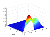
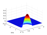
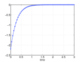
Fig. 6.1: Test 1: Uncontrolled solution (left), LQR optimal solution (middle), LQR optimal control (right).

Since our problem is linear-quadratic, the solution of the HJB equation can be computed by solving the well-known Riccati’s equation (for LQR approach see [14]). Then, the optimal LQR state is presented in the middle of Figure 6.1, whereas the optimal LQR control is plotted on the right of Figure 6.1. Then, we show the controlled solution computed by means of Algorithm 5.1 on the left of Figure 6.2.

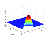
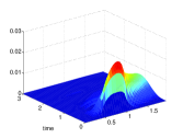
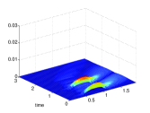
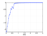
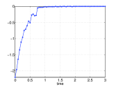
Fig. 6.2: Test 1: Optimal HJB states computed with Algorithm 5.1 with $\ell=4$ POD basis functions (top-left), difference between optimal solution with 4 POD basis and 2 POD basis (top-middle), difference between optimal solution with 4 POD basis and 3 POD basis (top-right), optimal HJB controls with $\ell=2,3,4$ (bottom).

Since it is hard to visualize differences from the optimal solutions we plot the difference between the optimal solution obtained with 4 POD basis functions and 2 POD basis in the middle of Figure 6.2 and with 3 POD basis on the right side. Nevertheless, one can even have a look at the error analysis in Figure 6.3.

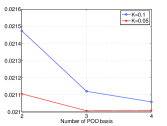
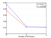
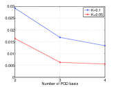
Fig. 6.3: Test 1: Evaluation of the cost functional (left), $L^{2}-$error for $y(u^{\ell})$ and $y^{\ell}(u^{\ell})$ (middle) and $L^{2}$-error between LQR solution and $y(u^{\ell})$. The blue line refers to the approximation with $K=0.1$ in HJB, whereas the red one to $K=0.05$.

In order to analyze our numerical approximation we consider the evaluation of the cost functional $\widehat{J}(u^{\ell};y_{\circ})$, the distance between $y(u^{\ell})$ and $y^{\ell}(u^{\ell})$ and the error between the truth solution and the suboptimal $y(u^{\ell})$. The error analysis is shown in Figure 6.3. On the left we show the decay of the cost functional when we increase the number of POD basis functions. In the middle we compute the $L^{2}-$error between the optimal reduced solution $y^{\ell}(u^{\ell})$ and the suboptimal solution $y(u^{\ell})$. Even in this case the error decays when $\ell$ increases and $K$ decreases. This error measures the quality of the surrogate model, since we want to check whether the suboptimal control fits into the non-reduced problem. Finally, on the right, we compute the error between the optimal solution and the suboptimal $y(u^{\ell})$. As expected, increasing the number of basis function and decreasing the step size $K$ (remember $h$ and $K$ are linked) for the approximation of the value function the optimal solution is improved.

The decay of the singular values is presented in Figure 6.4. As we can see they do not decay really fast with respect to the right plot which refers to the next example where the convection term is not dominated.
Finally, we want to give an idea of the term $\sup_{y\in\overline{\Omega}}{\|y-\mathcal{P}^{\ell}y\|}_{2}/h$ in the error estimate (4.19). It is clear we do not know $\Omega$, but we chose several randomly control sequences in the set of admissible controls. in order to have an approximation of the set. Now, we can compute the aforementioned error term. The decay is shown on the right of Figure 6.4.

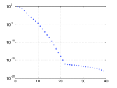
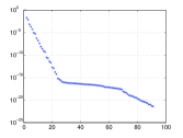
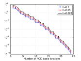
Fig. 6.4: Decay of the singular values for the snapshots set associated with Test 1 (left) and Test 2 (right).

6.2 Test 2: Semi-linear equation

The second test concerns the semi-linear equation. In (6.1) we set ${t_{\mathsf{e}}}=3$, $\varepsilon=10^{-1}$, $\gamma=0.1$, $\mu=1$, $\omega=(0,1)$ and $w_{\circ}(x)=2(x-x^{2})$. The shape function $b$ is equal to the initial condition $w_{\circ}$. In (6.2) we choose $\lambda=1$, and $\bar{w}=0$. To compute the POD basis we determine solutions to the state equation for controls in the set $U_{\mbox{snap}}=\{-1,0,1\}$ with a semi-implicit finite difference scheme with time step of $0.05$ and space step of $0.01$. In (4.11) we consider $K\in\{0.1,0.05\},h=0.1K$. The optimal trajectory is obtained with a time step size of $0.05$. The control set is given by 21 controls equally distributed from -1 to 1. The shape function $b$ is equal to the initial condition $w_{\circ}$.

The uncontrolled solution is shown on the left of Figure 6.5.

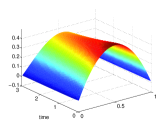
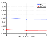
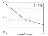
Fig. 6.5: Test 2: Uncontrolled solution (left), evaluation of the cost functional (middle) and distance between $y(u^{\ell})$, $y^{\ell}(u^{\ell})$ (right).

As we can see the semi-linear part does not allow to stabilize to zero the solution. Our goal is to steer the solution to the origin. The optimal solutions and its correspondent optimal controls are shown in Figure 6.6. Moreover we plot the differences between the computed solutions (please note the different scaling of the pictures). As we can see the difference decreases when the number of POD basis functions increase.

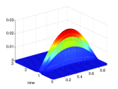
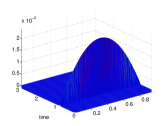
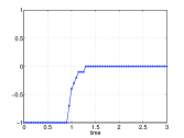
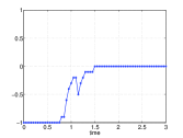
Fig. 6.6: Test 2: Optimal HJB states computed with Algorithm 5.1 with $\ell=4$ POD basis functions (top-left), difference between optimal solution with 4 POD basis and 2 POD basis (top-middle), difference between optimal solution with 4 POD basis and 3 POD basis (top-right), optimal HJB controls with $\ell=2,3,4$ (bottom).

The quality of our approximation is confirmed by Figure 6.5 where we can see from the evaluation of the cost functional and consistency of the suboptimal control. In this case the error decays much faster than in the previous example. This depends on the decay of the singular value of the snapshots set as shown in Figure 6.4.

6.3 Test 3: Semi-linear equation with uniform noise

In this test we deal with the semi-linear equation discussed in the previous example but we neglect the convection term ($\gamma=0$) and we add noise to the optimal trajectory. The uncontrolled solution is shown on the left of Figure 6.7, the optimal trajectory and control computed by means of Algorithm 5.1 are in the middle and the right side of Figure 6.7.

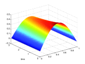
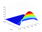
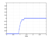
Fig. 6.7: Test 3: Uncontrolled solution (left), Optimal state (middle) and corresponding optimal HJB control (right).

The goal is to show the stabilization of the feedback control under strong perturbations of the system. We note that in this case the value function is stored from the system without perturbation, but the reconstruction of the feedback control is affected by uniform noise $\eta(x)$ between $[-1,1]$ in every time step: $y(x,\cdot)=(1+\eta(x))y(x,\cdot)$. Figure 6.8 shows optimal solution and control corresponding to different noise levels ($|\eta(x)|\leq 50\%$ (top) and $|\eta(x)\leq 90|\%$ (bottom)).

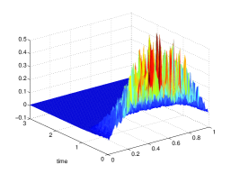
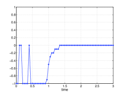
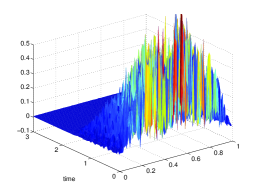
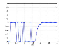
Fig. 6.8: Test 3: Optimal HJB-POD state (left) and corresponding optimal control (right) with $|\eta(x)|\leq 50\%$ (top) and $|\eta(x)|\leq 90\%$ noise (bottom).

In this example we can see the power of the feedback control, and in particular, the importance of the knowledge of the value function. In both examples, the trajectory is stabilized close to the origin. If we have a look at the optimal control input we can observe a strong chattering. In both cases the optimal control jumps often from -1 to 0. In particular, in the second case, it is possible to observe a stronger chattering due to the high disturbances. Nevertheless, the feedback control is able to stabilize the perturbed system.

7 Conclusion and Remarks

In this paper we present a new a-priori error analysis for the coupling between the HJB equation and the POD method. The proposed estimate is presented for the infinite horizon control problems with linear and nonlinear dynamical systems but this approach could be also applied to other optimal control problems provided one has a priori estimates on the approximation based on the HJB equation. The convergence of the method is guaranteed under rather general assumptions on the optimal control problem and some technical assumptions on the dynamics and on the POD approximation. For the latter, it is clear that a clever choice of the snapshots set can play a crucial role in the estimate in order to reduce the contribution of the POD approximation in the a-priori estimate. Several choices are possible based on greedy techniques or on a previous open-loop approximation, these choices will be investigated in a future paper. At present, the numerical tests illustrated in the last section confirms our theoretical findings and show the robustness of the Bellman’s approach also under strong disturbances of the dynamical system.

References

• [1] A. Alla and M. Falcone. An adaptive POD approximation method for the control of advection-diffusion equations, in K. Kunisch, K. Bredies, C. Clason, G. von Winckel, (eds) Control and Optimization with PDE Constraints, International Series of Numerical Mathematics, 164, Birkhäuser, Basel, 2013, 1-17.
• [2] A. Alla and M. Falcone. A time-adaptive POD method for optimal control problems, in the Proceedings of the 1st IFAC Workshop on Control of Systems Modeled by Partial Differential Equations, 1, 2013, 245-250.
• [3] A. Alla, M. Falcone, and D. Kalise. An accelerated value/policy iteration scheme for the solution of DP equations, in A. Abdulle, S. Deparis, D. Kressner, F. Nobile, M. Picasso (eds.), Numerical Mathematics and Advanced Applications, Proceedings of ENUMATH 2013, Lecture Notes in Computational Science and Engineering, 103, 2015, 489-497
• [4] A. Alla, M. Falcone, and D. Kalise. An efficient policy iteration algorithm for dynamic programming equations, SIAM J. Sci. Comput., 37, 2015, 181-200.
• [5] A. Alla and M. Hinze. HJB-POD feedback control for Navier-Stokes equations, Conference Proceeding ECMI, 2014.
• [6] A. Alla and M. Hinze. HJB-POD feeback control of advection-diffusion equation with a model predictive control snapshot sampling. , submitted, 2015.
http://preprint.math.uni-hamburg.de/public/papers/hbam/hbam2015-15.pdf
• [7] J.A. Atwell and B.B. King. Proper orthogonal decomposition for reduced basis feedback controllers for parabolic equations, Matematical and Computer Modelling, 33, 2001, 1-19.
• [8] M. Bardi and I. Capuzzo-Dolcetta. Optimal Control and Viscosity Solutions of Hamilton-Jacobi-Bellman Equations. Birkhäuser, Basel, 1997.
• [9] M. Barrault, Y. Maday, N.C. Nguyen, and A.T. Patera. An ’empirical interpolation’ method: application to efficient reduced-basis discretization of partial differential equations, Comptes Rendus Mathematique, 339, 2004, 667-672.
• [10] S. Cacace, E. Cristiani. M. Falcone, and A. Picarelli. A patchy dynamic programming scheme for a class of Hamilton-Jacobi-Bellman equations, SIAM Journal on Scientific Computing, 34, 2012, A2625-A2649.
• [11] F. Camilli, M. Falcone, P. Lanucara, and A. Seghini. A domain decomposition method for Bellman equations, in D. E. Keyes and J. Xu (eds.), Domain Decomposition methods in Scientific and Engineering Computing, Contemporary Mathematics n.180, AMS, 1994, 477-483.
• [12] D. Chapelle, A. Gariah, and J. Saint-Marie. Galerkin approximation with proper orthogonal decomposition: new error estimates and illustrative examples, ESAIM: Math. Model. Numer. Anal., 46, 2012, 731-757.
• [13] S. Chaturantabut and D.C. Sorensen. Nonlinear model reduction via discrete empirical interpolation, SIAM Journal on Scientific Computing, 32, 2010, 2737-2764.
• [14] R.F. Curtain and H.J. Zwart. An Introduction to Infinite-Dimensional Linear Systems Theory, Springer, 1995.
• [15] M. Falcone. A numerical approach to the infinite horizon problem of deterministic control theory, Applied Mathematics and Optimization, 15, 1987, 1-13.
• [16] M. Falcone. Numerical solution of dynamic programming equations, Appendix A of [8], Birkhäuser, Basel, 1997.
• [17] M. Falcone and R. Ferretti. Semi-Lagrangian Approximation Schemes for Linear and Hamilton-Jacobi equations, SIAM, 2014.
• [18] M. Falcone, P. Lanucara, and A. Seghini. A splitting algorithm for Hamilton-Jacobi-Bellman equations Applied Numerical Mathematics, 15, 1994, 207-218.
• [19] W.H. Fleming and H.M. Soner. Controlled Markov processes and viscosity solutions, Springer-Verlag, New York, 1993.
• [20] R. Glowinski, J.L. Lions, and R. Trémolières. Analyse Numerique des Inéquations Variationelles, Dunod-Bordas, Paris, 1976.
• [21] M. Gubisch and S. Volkwein. Proper orthogonal decomposition for linear-quadratic optimal control, submitted, 2013.
http://kops.ub.uni-konstanz.de/handle/urn:nbn:de:bsz:352-250378
• [22] P. Holmes, J.L. Lumley, G. Berkooz, and C.W. Rowley. Turbulence, Coherent Structures, Dynamical Systems and Symmetry, Cambridge Monographs on Mechanics, Cambridge University Press, second edition, 2012.
• [23] M. Hinze, R. Pinnau, M. Ulbrich, and S. Ulbrich. Optimization with PDE Constraints. Mathematical Modelling: Theory and Applications, 23, Springer Verlag, 2009.
• [24] M. Hinze and S. Volkwein. Proper orthogonal decomposition surrogate models for nonlinear dynamical systems: error estimates and suboptimal control, in Reduction of Large-Scale Systems, P. Benner, V. Mehrmann, D. C. Sorensen (eds.), Lecture Notes in Computational Science and Engineering, 45, 2005, 261-306.
• [25] D. Kalise and A. Kröner. Reduced-order minimum time control of advection-reaction-diffusion systems via dynamic programming, In Proceedings of the 21st International Symposium on Mathematical Theory of Networks and Systems, 2014, 1196-1202.
• [26] K. Kunisch and S. Volkwein. Galerkin proper orthogonal decomposition methods for a general equation in fluid dynamics, SIAM Journal on Numerical Analysis, 40, 2002, 492-515.
• [27] K. Kunisch, S. Volkwein, and L. Xie. HJB-POD based feedback design for the optimal control of evolution problems, SIAM J. on Applied Dynamical Systems, 4, 2004, 701-722.
• [28] K. Kunisch and L. Xie. POD-based feedback control of Burgers equation by solving the evolutionary HJB equation, Computers and Mathematics with Applications, 49, 2005, 1113-1126.
• [29] F. Leibfritz and S. Volkwein. Reduced order output feedback control design for PDE systems using proper orthogonal decomposition and nonlinear semidefinite programming, Linear Algebra and Its Applications, 415, 2006, 542-575.
• [30] J.L. Lions. Optimal Control of Systems Governed by Partial Differential Equations, Springer-Verlag, New York 1971.
• [31] C. Navasca and A. J. Krener. Patchy solutions of Hamilton-Jacobi-Bellman partial differential equations, in A. Chiuso et al. (eds.), Modeling, Estimation and Control, Lecture Notes in Control and Information Sciences, 364 2007, 251-270.
• [32] A. Quarteroni and A. Valli. Domain Decomposition Methods for Partial Differential Equations, Oxford University Press, 1999.
• [33] E.W. Sachs and S. Volkwein. POD Galerkin approximations in PDE-constrained optimization, GAMM Mitteilungen, 33, 2010, 194-208.
• [34] J. A. Sethian. Level set methods and fast marching methods, Cambridge University Press, 1999.
• [35] J. A. Sethian and A. Vladimirsky. Ordered upwind methods for static Hamilton-Jacobi equations: theory and algorithms, SIAM J. Numer. Anal., 41, 2003, 325-363.
• [36] J.R. Singler. New POD expressions, error bounds, and asymptotic results for reduced order models of parabolic PDEs, SIAM Journal on Numerical Analysis, 52, 2014, 852-876.
• [37] Y. Tsai, L. Cheng, S. Osher, and H. Zhao. Fast sweeping algorithms for a class of Hamilton-Jacobi equations, SIAM J. Numer. Anal., 41, 2004, 673-694.
• [38] F. Tröltzsch. Optimal Control of Partial Differential Equations: Theory, Methods and Application, American Mathematical Society, 2010.
• [39] S. Volkwein. Model Reduction using Proper Orthogonal Decomposition, Lecture Notes, University of Konstanz, 201.
http://www.math.uni-konstanz.de/numerik/personen/volkwein/teaching/scripts.php