A Kinematic Condition on Intrinsic Charm

Johannes Blümlein

Deutsches Elektronen–Synchrotron, DESY,
Platanenallee 6, D-15738 Zeuthen, Germany

Abstract

We derive a kinematic condition on the resolution of intrinsic charm and discuss phenomenological consequences.

Intrinsic charm in nucleons has been proposed as a phenomenon, which can be described in the light-cone wave function formalism [1] using old fashioned perturbation theory [2]. It is characterized by a Fock state

$$|q_{1}\,q_{2}\,q_{3}\,Q_{4}\,Q_{5}\rangle,$$ (1)

with massless quarks $q_{i}$ and heavy quarks $Q_{j}$ of mass $M_{Q}$.. The emergence of this state can be viewed as a definite quantum fluctuation in front of a general hadronic background, which can be resolved in deep-inelastic lepton-nucleon scattering.

Extrinsic heavy flavor contributions [4, 5], on the other hand, are due to factorized single massless parton induced processes, exciting the heavy quark contributions. For neutral current interactions the process results from vector boson-gluon fusion [4] and appears in first order in the strong coupling constant $\alpha_{s}$ at the quantum level.

Both processes are distinct and of very different nature. As has been shown in Ref. [1] the intrinsic charm contributions are situated at larger values of $x$, while major contributions of the extrinsic charm appear at low values of $x$. While the intrinsic charm contribution appears in the scaling limit already, extrinsic charm contributes on the quantum level only.

In the following we derive the condition under which intrinsic charm is unambiguously visible in deep-inelastic scattering. We follow Drell and Yan, Ref. [6], and compare the lifetime, $\tau_{\rm life}$, of the intrinsic charm state with the interaction time in the deep-inelastic process, $\tau_{\rm int}$, demanding

$$\frac{\tau_{\rm life}}{\tau_{\rm int}}\gg 1$$ (2)

as a necessary criterion for the observation of the phenomenon. Eq. (2) delivered a clear condition on the applicability of the (massless) parton model singling out the corresponding ranges in $x$ and $Q^{2}$. Here the major requests are that the virtuality $Q^{2}$ of the process is much larger than any transverse momentum squared in the hadronic wave-function, $Q^{2}\gg k_{\perp,i}^{2}$, and the Bjorken variable $x$ shall neither get close to 1 nor take too small values, [6]. Usually, in the excluded regions other contributions, like higher twist terms are present and/or there is a need of novel small-$x$ resummations, which are both of comparable or even of larger size than the terms computed. In the following we will apply Eq. (2) to the case of the state (1).

In an infinite momentum frame we may express the momentum transfer by the electro-weak boson probing the nucleon, $q$, as follows [6]

$$q=(q_{0};q_{3},q_{\perp}),\leavevmode\nobreak\ \leavevmode\nobreak\ q_{0}=\frac{2m_{p}\nu+q^{2}}{4P},\leavevmode\nobreak\ \leavevmode\nobreak\ q_{3}=-\frac{2m_{p}\nu-q^{2}}{4P},$$ (3)

where $q^{2}=-Q^{2}$, $m_{p}$ the proton mass, $\nu$ the energy transfer to the nucleon in the proton rest frame, and $P$ is the large (‘infinite’) momentum.

The interaction time $\tau_{\rm int}$ is given by

$$\tau_{\rm int}=\frac{1}{q_{0}}=\frac{4P}{2m_{p}\nu+q^{2}}=\frac{4Px}{Q^{2}(1-x)}\leavevmode\nobreak\ .$$ (4)

Here $x$ denotes the momentum fraction of the struck quark. Likewise, we obtain for the lifetime of the intrinsic charm state

$$\tau_{\rm life}=\frac{1}{\sum_{i}E_{i}-E}=\left.\frac{2P}{\left(\sum_{i=1}^{5}\frac{M_{i}^{2}+k_{\perp,i}^{2}}{x_{i}}\right)-m_{p}^{2}}\right|_{\sum_{j}x_{j}=1},$$ (5)

with $E_{i}=\sqrt{x_{i}^{2}P^{2}+M_{i}^{2}+k_{\perp,i}^{2}}$ the energies of the partons in the state and $E$ the total energy, applying the infinite momentum representation, consistently neglecting sub-leading terms $\sim 1/P$ in the large momentum. $M_{i}$ denotes the mass of the $i$th quark, $k_{\perp,i}$ its transverse momentum, and $x_{i}$ its momentum fraction. Deriving $\tau_{\rm life}$ for intrinsic charm, we consider three massless valence quarks and the heavy quark-antiquark pair in the Fock state. We set the masses of the three light valence quarks to zero and neglect the effect of transverse momenta, as in the derivation of Eq. (8) [1], but retain the term $m_{p}^{2}/M_{Q}^{2}$ here. One obtains

$$\tau_{\rm life}(x) = \left.\frac{2P}{M_{Q}^{2}}\int_{0}^{1-x_{5}}dx_{4}\int_{0}^{1-x_{4}-x_{5}}dx_{3}\frac{1-x_{3}-x_{4}-x_{5}}{\frac{1}{x_{4}}+\frac{1}{x_{5}}-\frac{m_{p}^{2}}{M_{Q}^{2}}}\right|_{x_{5}=x}$$ (6)

$$= \frac{Px}{6M_{Q}^{2}(1-cx)^{4}}\Biggl{\{}(1-x)(1-cx)[2+x[5-x-c(1-x)[4+x(5-2c(1-x))]]]$$

$$+6x(1-cx(1-x))^{2}\ln\left[\frac{x}{1-cx(1-x)}\right]\Biggr{\}},$$

with $c=m_{p}^{2}/M_{Q}^{2}$. The integrals in (6) are the same as used to derive the probability distribution $P(x)$ in [1] and Eq. (9), however, the energy denominator appears in the first power.

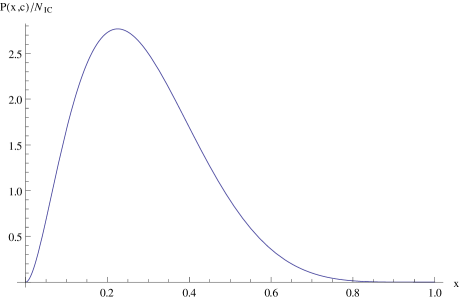
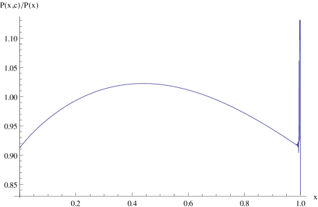
Figure 1: Left panel: Normalized intrinsic charm distribution with finite $m_{p}$; Right panel: ratio of the probability distribution for intrinsic charm including the effect of the proton mass to the case $m_{p}/M_{Q}\rightarrow 0$. The parameter $c$ is given by $c\simeq 0.348$ and $M_{Q}=1.59\leavevmode\nobreak\ \rm GeV$ in the pole mass scheme [7]. 

One may estimate also a lifetime for extrinsic $c\bar{c}$-production, if viewed as Fock state. Due to the factorized production, one considers the state $|c\bar{c}X\rangle$, with $X$ the hadronic remainder of momentum fraction $x_{1}$, which yields

$$\tau_{\rm life}^{\rm ext}(x) = \left.\frac{2P}{M_{Q}^{2}}\int_{0}^{1}dx_{4}\int_{0}^{1}dx_{1}\delta(1-x_{1}-x_{4}-x_{5})\frac{1}{\frac{1}{x_{4}}+\frac{1}{x_{5}}-c}\right|_{x_{5}=x}$$ (7)

$$= \frac{2Px}{M_{Q}^{2}(1-cx)^{2}}\left\{(1-x)(1-cx)+x\ln\left[\frac{x}{1-cx(1-x)}\right]\right\}\leavevmode\nobreak\ .$$

The lowest order probability distribution for intrinsic charm, accounting for the nucleon mass effect, is given by

$$P(x) = \left.N(c)\int_{0}^{1-x_{5}}dx_{4}\int_{0}^{1-x_{4}-x_{5}}dx_{3}\frac{1-x_{3}-x_{4}-x_{5}}{\left(\frac{1}{x_{4}}+\frac{1}{x_{5}}-c\right)^{2}}\right|_{x_{5}=x}$$ (9)

$$= \frac{N(c)x^{2}}{6(1-cx)^{5}}\Biggl{\{}(1-x)(1-cx)[1+x[10+x-c(1-x)(x(10-c(1-x))+2)]]$$

$$+6x[1+x(1-c(1-x))][1-c(1-x)x][\ln(x)-\ln[1-c(1-x)x]]\Biggr{\}},$$

with $N(c)$ determined such that $\int_{0}^{1}dxP(x)=N_{\rm IC}$, the integral fraction of intrinsic charm. Here we retained the effect of the proton mass, which was neglected in [1], and illustrate the distribution in Figure 1a. One obtains a modification of the intrinsic charm distribution due to the finite nucleon mass effect of up to 10%, as shown in see Figure 1b. Setting $c\rightarrow 0$ leads to the previous result [1]

$$P(x) = 600N_{\rm IC}x^{2}\Biggl{[}(1-x)(x^{2}+10x+1)+6x(x+1)\ln(x)\Biggr{]}\leavevmode\nobreak\ .$$ (10)

The ratio $\rho(x)=\tau_{\rm life}/\tau_{\rm int}$ is Lorentz-invariant and has to be larger than a suitable bound of $O(5...10)$. The size of this value is fixed using standard requests applied also for the parameter setting in experimental pulse resolution techniques e.g. in particle detectors. Here $\rho=5$ would refer to a failure rate of 20% and $\rho=10$ of 10%.

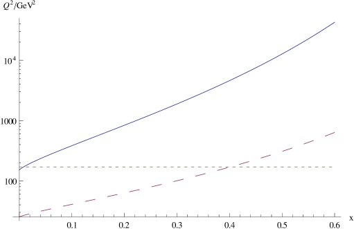
Figure 2: Full line: lower boundary in $Q^{2}/\rm GeV^{2}$ for which $\rho(x)\geq 5$ as a function of $x$. Long dashed line: lower boundary for extrinsic charm production resulting from Eq. (7) also for $\rho(x)\geq 5$; Short dashed line: highest $Q^{2}$-bin of the EMC experiment [9].

Using this condition we may determine the allowed $Q^{2}$-range as a function of $x$ in which the quantum fluctuation leading to intrinsic charm can be unambiguously resolved by deep-inelastic scattering. Eqs. (4,6) lead to the function

$$\rho(x)\equiv\frac{\tau_{\rm life}(x)}{\tau_{\rm int}(x)}\geq\frac{Q^{2}}{12M_{Q}^{2}}\simeq\frac{Q^{2}}{30.34\leavevmode\nobreak\ \rm GeV^{2}}.$$ (11)

The function $\rho(x)$ rises with growing values of $x$, i.e. a minimal bound of $Q^{2}>151\leavevmode\nobreak\ \rm GeV^{2}$ is obtained, demanding the ratio to be $\rho(x)\geq 5$. We show the corresponding $x$-dependence in Figure 2. We also show the boundary implied for extrinsic charm production.

Let us consider the kinematics of the EMC experiment at CERN [9], which probably was the first measuring charm final states of a larger amount in deep-inelastic scattering [10]. These data have frequently been analyzed also searching for intrinsic charm. The highest $Q^{2}$ bin is centered at $Q^{2}\simeq 170\leavevmode\nobreak\ \rm GeV^{2}$. The kinematic range allowed for a clear intrinsic charm signal demanding $\rho(x)\geq 5$ is obtained as $x\raisebox{-1.9919pt}{$\,\stackrel{{\scriptstyle<}}{{{\scriptstyle\sim}}}\,$}0.01$, far below the peak-region at $x\simeq 0.22$ of the predicted distribution. On the other hand, the bound resulting for extrinsic charm production, cf. Eq. (7), covers a wider range, also of the kinematic region probed by the EMC experiment. Note that, furthermore, the accessible range in $x$ is strongly correlated to the probed region in $Q^{2}$ in deep-inelastic scattering experiments. This has to be taken into account interpreting low energy data as those of the EMC experiment in terms of intrinsic charm effects. Several phenomenological analyses have been carried out to search for intrinsic charm, cf. e.g. Refs. [11]. Other analyses came to very similar conclusions of a possible integral fraction of $N_{\rm IC}$ in the range of up to $O(1..3\%)$. In all these analyses the life-time constraint (2) has not been considered.

Discoveries need clean conditions. The $Q^{2}$ bound illustrated by Figure 2 points to a much more fortunate situation to search for intrinsic charm effects opening up at high energy colliders if compared to fixed target experiments, such as at HERA or within future projects like the EIC [12] and LHeC [13], also operating at high luminosity. Condition (2) is more easily fulfilled there because of the much wider kinematic range. As a consequence, intrinsic charm can be searched for in a dedicated way only at high energies.

Acknowledgment.  I would like to thank H. Fritzsch and G. Branco for organizing a nice conference on High Energy Physics in the beautiful Algarve, where this note has been worked out. Conversations with S. Brodsky and M. Klein are gratefully acknowledged. This work was supported in part by the European Commission through contract PITN-GA-2012-316704 (HIGGSTOOLS).

References

- [1] S.J. Brodsky, P. Hoyer, C. Peterson and N. Sakai, Phys. Lett. B 93 (1980) 451.
- [2] S. Weinberg, Phys. Rev. 150 (1966) 1313, Erratum: 158 (1967) 1638.
- [3] E. Hoffmann and R. Moore, Z. Phys. C 20 (1983) 71.
- [4] E. Witten, Nucl. Phys. B 104 (1976) 445.
-
[5]
E. Laenen, S. Riemersma, J. Smith and W.L. van Neerven,
Nucl. Phys. B 392 (1993) 162,
229;
J. Blümlein, A. DeFreitas and C. Schneider, Nucl. Part. Phys. Proc. 261-262 185 [arXiv:1411.5669 [hep-ph]] and references therein. - [6] S.D. Drell and T.M. Yan, Annals Phys. 66 (1971) 578.
-
[7]
S. Alekhin, J. Blümlein, K. Daum, K. Lipka and S. Moch,
Phys. Lett. B 720 (2013) 172
[arXiv:1212.2355 [hep-ph]];
K.A. Olive et al. (Particle Data Group), Chin. Phys. C 38 (2014) 090001. - [8] S. Dulat, T. J. Hou, J. Gao, J. Huston, J. Pumplin, C. Schmidt, D. Stump and C.-P. Yuan, Phys. Rev. D 89 (2014) 7, 073004 doi:10.1103/PhysRevD.89.073004 [arXiv:1309.0025 [hep-ph]].
- [9] J.J. Aubert et al. [European Muon Collaboration], Nucl. Phys. B 259 (1985) 189.
- [10] J.J. Aubert et al. [European Muon Collaboration], Nucl. Phys. B 213 (1983) 31.
-
[11]
B.W. Harris, J. Smith and R. Vogt,
Nucl. Phys. B 461 (1996) 181
[hep-ph/9508403];
P. Jimenez-Delgado, T. J. Hobbs, J. T. Londergan and W. Melnitchouk, Phys. Rev. Lett. 114 (2015) 8, 082002 [arXiv:1408.1708 [hep-ph]];
S.J. Brodsky and S. Gardner, arXiv:1504.00969 [hep-ph];
P. Jimenez-Delgado, T. J. Hobbs, J. T. Londergan and W. Melnitchouk, arXiv:1504.06304 [hep-ph]. -
[12]
D. Boer, M. Diehl, R. Milner, R. Venugopalan, W. Vogelsang, D. Kaplan, H. Montgomery, S. Vigdor et al.,
arXiv:1108.1713 [nucl-th];
A. Accardi, J.L. Albacete, M. Anselmino, N. Armesto, E.C. Aschenauer, A. Bacchetta, D. Boer, W. Brooks et al., arXiv:1212.1701 [nucl-ex]. - [13] J.L. Abelleira Fernandez et al. [LHeC Study Group Collaboration], J. Phys. G 39 (2012) 075001 [arXiv:1206.2913 [physics.acc-ph]].