Recent progress in hadron structure from Lattice QCD

Abstract:

We review recent progress in hadron structure using lattice QCD simulations, with main focus in the evaluation of nucleon quantities such as the axial and tensor charges, and the spin content of the nucleon, using simulations at pion masses close to the physical value. We highlight developments on the evaluation of the gluon moment, a new direct approach to compute quark parton distributions functions on the lattice, as well as, the neutron electric dipole moment. A discussion of the systematic uncertainties and the computation of the disconnected contributions using dynamical simulations is also included.

1 Motivation

Lattice QCD (LQCD) is a non-perturbative approach that provides a powerful tool for ab initio evaluation of hadron observables. These include both quantities that are well determined experimentally, but also those that are not easily accessible in experiment. Thus, LQCD provides input to phenomenology and to searches for beyond the Standard Model Physics. Recent progress in the simulation of LQCD has been impressive, mainly due to the improvements in the algorithms, development of new techniques, and increase in computational power. This enabled simulations to be carried out at parameters very close to their physical values.

Understanding nucleon structure from first principles is considered a milestone of hadron physics and numerous experiments have been devoted to its study, starting with the measurements of the electromagnetic form factors initiated more than 50 years ago. Reproducing these key observables within the lattice QCD formulation is a prerequisite to obtaining reliable predictions on observables that explore Physics beyond the Standard Model. There is a rich experimental program in major facilities (CERN, JLab, MAMI, MESA, PSI, JPARC, etc) investigating hadron structure, such as the proton radius, electric dipole moments and scalar and tensor interactions.

The 12 GeV upgrade of the Continuous Electron Beam Accelerator Facility at JLab will allow to employ new methods for studying the basic properties of hadrons. Hadron structure has been an essential part of the physics program, which involves new and interesting high precision experiments, such as nucleon resonance studies with CLAS12, the longitudinal spin structure of the nucleon, meson spectroscopy with low momentum transfer electron scattering, high precision measurement of the proton charge radius, and many more.

The experiments on the proton radius have attracted a lot of interest since accurate measurements of the root mean square charge radius from muonic hydrogen [1] ($\langle r^{2}_{p}\rangle_{\mu H}=0.84\,{\rm fm}^{2}$) is 7.7$\sigma$ yielded a value smaller that the radius determined from elastic e-p scattering and hydrogen spectroscopy ($\langle r^{2}_{p}\rangle_{ep}=0.88\,{\rm fm}^{2}$) [3] (see Ref. [2] for a review). The 4$\%$ difference in the two measurements is currently not explained. We note that the measurements in the muonic hydrogen experiments are ten times more accurate than other measurements and they are very sensitive to the proton size. In particular, the radius is measured from the energy difference between the 2P and 2S states of the muonic hydrogen [4] and more accurate experiments are planned at PSI.

The above few examples illustrate that hadron structure is a very rich field of research relevant to new physics searches. Thus, lattice QCD does not only provide input to on-going experiments, but also gives guidance to new experiments within a robust theoretical framework.

Being one of the building-blocks in the universe, the nucleon provides an extremely valuable laboratory for studying strong dynamics providing important input that can also shed light in new physics searches. Although it is the only stable hadron in the Standard Model, its structure is not fully understood yet. There have been several recent lattice QCD results on nucleon observables. In these proceedings we discuss representative observables probing hadron structure, as well as, challenges involved in their computations. Topics to be covered include the nucleon axial and tensor charges, the nucleon spin, including disconnected contributions, neutron electric dipole moment, the first gluon moment of parton distribution functions (PDFs), and a direct method for computing quasi-distribution functions on the lattice. The systematic uncertainties related to nucleon matrix elements are also investigated.

2 Nucleon Matrix Elements

In the evaluation of nucleon matrix elements in LQCD there are two type of diagrams entering, shown in Fig. 1. The disconnected diagram has been neglected in most of the studies because it is very noisy and expensive to compute. However, in the last few years a number of groups are studying various techniques for its computation using dynamical simulations.

         

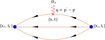
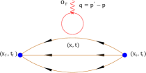
Figure 1: Connected (left) and disconnected (right) contributions to the nucleon three-point function.

For the computation of nucleon matrix elements one constructs two- and three-point correlation functions defined as

$$G^{2pt}(\vec{q},t_{f}) = \sum_{\vec{x}_{f}}\,e^{-i\vec{x}_{f}\cdot\vec{q}}\,\Gamma^{0}_{\beta\alpha}\,\langle{{J_{\alpha}(\vec{x}_{f},t_{f})}}{{\overline{J}_{\beta}(0)}}\rangle\,,$$ (1)

$$G^{3pt}_{\cal O}(\Gamma^{\mu},\vec{q},t_{f}) = \sum_{\vec{x}_{f},\vec{x}}\,e^{i\vec{x}\cdot\vec{q}}\,e^{-i\vec{x}_{f}\cdot\vec{p}^{\prime}}\Gamma^{\mu}_{\beta\alpha}\,\langle{J_{\alpha}(\vec{x}_{f},t_{f})}{\cal O}(\vec{x},t){\overline{J}_{\beta}(0)}\rangle\,,$$ (2)

appropriately projected in order to compute the quantities of interest. For instance, the projectors $\Gamma^{\mu}$ are usually defined as $\Gamma^{0}\equiv\frac{1}{4}(1+\gamma_{0}),\,\,\Gamma^{k}\equiv\Gamma^{0}\cdot\gamma_{5}\cdot\gamma_{k}\,$. The lattice data are extracted from dimensionless ratio of the two- and three-point correlation functions

$$R_{\cal O}(\Gamma,\vec{q},t,t_{f}) {=} \frac{G^{3pt}_{\cal O}(\Gamma,\vec{q},t)}{G^{2pt}(\vec{0},t_{f})}\times\sqrt{\frac{G^{2pt}({-}\vec{q},t_{f}{-}t)G^{2pt}(\vec{0},t)G^{2pt}(\vec{0},t_{f})}{G^{2pt}(\vec{0},t_{f}{-}t)G^{2pt}({-}\vec{q},t)G^{2pt}({-}\vec{q},t_{f})}}\,\,{\rightarrow\atop{{t_{f}{-}t\rightarrow\infty}\atop{t{-}t_{i}\rightarrow\infty}}}\,\,\Pi(\Gamma,\vec{q})\,.$$ (3)

The above ratio is considered optimized since it does not contain potentially noisy two-point functions at large separations and also correlations between its different factors reduce the statistical noise. The most common method to extract the desired matrix element is to look for a plateau with respect to the current insertion time, $t$ (or, alternatively, the sink time, $t_{f}$), which should be located at a time well separated from the creation and annihilation times in order to ensure single state dominance. To establish proper connection to experiments we apply renormalization which, for most of the quantities discussed in this review, is multiplicative

$$\Pi^{R}(\Gamma,\vec{q})=Z_{\cal O}\,\Pi(\Gamma,\vec{q})\,.$$ (4)

The renormalized matrix elements can be parameterized in terms of Generalized Form Factors (GFFs), and the decomposition follows the symmetry properties of QCD. As an example we take the axial current insertion, which decomposes into two Lorentz invariant Form Factors (FFs), the axial ($G_{A}$) and induced pseudoscalar ($G_{p}$)

$$\langle N(p^{\prime},s^{\prime})|\bar{\psi}(x)\,\gamma_{\mu}\,\gamma_{5}\,\psi(x)|N(p,s)\rangle=i\Bigg{(}\frac{m_{N}^{2}}{E_{N}({\bf p}^{\prime})E_{N}({\bf p})}\Bigg{)}^{1/2}\bar{u}_{N}(p^{\prime},s^{\prime})\Bigg{[}G_{A}(q^{2})\gamma_{\mu}\gamma_{5}+\frac{q_{\mu}\gamma_{5}}{2m_{N}}G_{p}(q^{2})\Bigg{]}u_{N}(p,s)\,,$$ (5)

where $q^{2}$ is the momentum transfer in Minkowski space (hereafter, $Q^{2}=-q^{2}$).

Here, I will mostly consider the flavor isovector combination for which the disconnected contribution cancels out; strictly speaking, this happens for actions with exact isospin symmetry. Another advantage of the isovector combination is that the renormalization simplifies considerably.

2.1 Systematic uncertainties

The systematic uncertainties are important aspects of lattice computations that need to be addressed carefully. In a nutshell, such systematics are:

$\bullet$ cut-off effects due to the introduction of a finite lattice spacing. For a proper continuum extrapolation one requires simulations for, at least, three values of the lattice spacing, which is computationally very costly, especially as we approach the physical point. To minimize this systematic, gauge configurations are generated employing improved actions with a value of the lattice that ensures small or negligible cut-off effects compared to the statistical accuracy.

$\bullet$ finite volume effects due to the finite extent of the space-time box. These in general depend on the quantity under study. Ideally, simulations should be performed at multiple volumes, so that the infinite volume limit can be taken. This requires significant computer resources. As a rule of thumb one needs $L\,m_{\pi}$ larger than $3.5$ to suppress finite volume effects.

$\bullet$ contamination from other hadron states due to the fact that the interpolating field used to create a hadron of given quantum numbers couple in addition to states higher in energy. While for two-point functions identification of the lowest energy state is straight forward, for three-point functions it is more saddle, and there are various methods to extract information from lattice data. The most common approach is the so called plateau method in which one probes the large Euclidean time evolution of the ratio in Eq. (3)

$$R_{\cal O}(\Gamma,t_{i},t,t_{f}){\rightarrow\atop{{(t_{f}{-}t)\,\Delta>>1}\atop{(t{-}t_{i})\,\Delta>>1}}}\,\,{\cal M}\Bigg{[}1{+}\alpha\,e^{-(t_{f}{-}t)\,\Delta(p^{\prime})}{+}\beta\,e^{-(t{-}t_{i})\,\Delta(p)}{+}\cdots\Bigg{]}\,.$$ (6)

In the above equation the excited states contributions fall exponentially with the sink-insertion ($t_{f}-t$) and insertion-source ($t-t_{i}$) time separation. So, it is possible to reduce the unwanted excited states contamination by increasing the source-sink separation, but this comes with a cost of increased statistical noise.

Another method is the so-called summation method in which we sum the ratio from the source to the sink, and thus, the excited state contaminations are suppressed by exponentials decaying with $(t_{f}-t_{i})$ rather than $(t_{f}-t)$ and $(t-t_{i})$. However, one needs the slope of the summed ratio

$$\sum_{t=t_{i}}^{t_{f}}\,R(t_{i},t,t_{f})={\rm const.}+{\cal M}\,(t_{f}-t_{i})+{\cal O}\Bigg{(}e^{-((t_{f}-t_{i})\,\Delta(p^{\prime}))}\Bigg{)}+{\cal O}\Bigg{(}e^{-((t_{f}-t_{i})\,\Delta(p))}\Bigg{)}\,.$$ (7)

$\bullet$ simulations at unphysically large values of the pion mass due to limitations on the computational resources and optimization techniques. Then one typically uses chiral perturbation theory ($\chi$PT) to carry the extrapolation to the physical point, with low energy constants determined by over-constraining the fits using experimental, as well as, lattice data. Over the last years simulations at physical parameters have become feasible, which can be compared directly to experimental and phenomenological data. This is a substantial step forward since the chiral extrapolation to the physical point is avoided, which is often difficult and can lead to rather large systematic uncertainties, in particular in the baryon sector.

$\bullet$ renormalization, which might involve mixing with other observables. In addition the data should be converted to the $\overline{\rm MS}$ scheme in order to be compared to experimental and phenomenological data. This conversion is performed using perturbative expressions to finite order in the coupling constant and this might bring in systematic uncertainties; using higher-loop expressions (typically ${\cal O}(g^{6})$) exhibit very small systematics. More importantly, renormalization functions computed non-perturbatively may carry lattice artifacts, which can be removed by subtracting them utilizing perturbation theory [5, 6, 7].

3 Nucleon Charges

3.1 Axial Charge

One of the fundamental nucleon observables is the axial charge, $g_{A}\equiv G_{A}(0)$, which is determined from the forward matrix element of the axial current, and gives the intrinsic quark spin in the nucleon. It governs the rate of $\beta$-decay and has been measured precisely. In LQCD the axial charge can be determined directly from the evaluation of the matrix element and thus, there is no ambiguity associated to fits. For this reasons, $g_{A}$ is an optimal benchmark quantity for hadron structure computations, and it is essential for LQCD to reproduce its experimental value or if a deviation is observed to understand its origin.

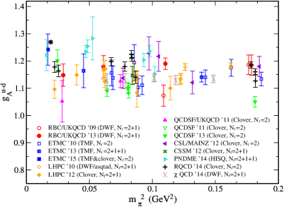
Figure 2: Collection of lattice results for $g_{A}$ corresponding to: $N_{f}{=}2{+}1$ DWF (RBC/UKQCD [12, 13], RBC/UKQCD [14], $\chi$QCD [15]), $N_{f}{=}2{+}1$ DWF on asqtad sea (LHPC [16]), $N_{f}{=}2$ TMF (ETMC [17]), $N_{f}{=}2$ Clover (QCDSF/UKQCD [18], CLS/MAINZ [19], QCDSF [20], RQCD [21]), $N_{f}{=}2{+}1$ Clover (LHPC [22], CSSM [23]), $N_{f}{=}2{+}1{+}1$ TMF (ETMC [24]), $N_{f}{=}2{+}1{+}1$ HISQ (PNDME [25, 26]), $N_{f}{=}2$ TMF with Clover (ETMC [27]). The asterisk is the experimental value [28].

There are numerous computations of $g_{A}$ from many collaborations and selected results are shown in Fig. 2 as a function of $m_{\pi}^{2}$. These results have been obtained using dynamical gauge field configurations with ${\cal O}(a)$-improved lattice QCD actions, namely Domain Wall Fermions (DWF), Hybrid, Clover, Twisted Mass Fermions (TMF) and HISQ fermions (see caption of Fig. 2 for references). For a meaningful comparison we include only results obtained from the plateau method without any volume corrections. The latest achievement of the Lattice Community are the results at the physical point for which there is no necessity of chiral extrapolation eliminating an up to now uncontrolled extrapolation. The ones at the two lowest values of the pion mass correspond to PNDME (128 MeV) [26] and ETMC (133 MeV) [27], and are in agreement with the experimental value: $g_{A}^{\rm exp}=0.2701(25)$ [28]. Of course the statistical errors are still large and it is necessary to increase the statistics and study the volume and lattice spacing dependence before finalizing these results. In addition, the results shown in Fig. 2 are at a given lattice spacing and volume and, thus, systematic effects should be investigated.

In summary, based on current results on the axial charge [29], we conclude that cut-off effects are small, at least for $a\leq 0.1$ fm, and no indication of significant excited state contamination has been observed indicating that sink-source time separation of about 1 fm is sufficient. No clear conclusion can be extracted regarding finite volume effects that need further investigation. It is worth stressing, however, that the value of $g_{A}$ determined close to the physical point by ETMC with $L\,m_{\pi}\sim 3$ ($a<0.1$ fm), and by PNDME with $L\,m_{\pi}\sim 3.75$ ($a<0.1$ fm) are in agreement with the experimental data.

We note that all high statistics studies of systematic uncertainties have been performed at relatively large values of the pion mass. It is thus essential to also perform similar investigations at values of the pion mass closer to the physical one. Given that the signal to noise error decreases exponentially as the pion mass decreases one needs to increase considerably the number of independent measurements leading to increase computational cost, and thus, noise reduction methods are highly valuable.

3.2 Tensor Charge

The nucleon scalar and tensor charges have not been studied in LQCD as extensively as $g_{A}$ since the contributions of effective scalar and tensor interactions in the Standard Model are very small (per-mil level). These interactions correspond to the non $V-A$ structure of weak interactions and serve as a test for new physics. Ongoing experiments using ultra-cold neutrons [30, 31, 32, 33], as well as planned ones [34] will reach the necessary precision to investigate such interactions.

In order to study the scalar and tensor interactions we add a term in the effective Hamiltonian corresponding to new BSM physics,

$$H_{eff}=G_{F}\left(J_{V_{A}}^{l}\times J_{V_{A}}^{q}+\sum_{i}\epsilon_{i}{\cal O}_{i}^{l}\times{\cal O}_{i}^{q}\right)$$ (8)

where the sum includes operators with novel structure, such as the scalar and tensor, which come with low-energy couplings that are related to masses of new TeV-scale particles.

Experimentally, bounds on the tensor coupling constant arise in the radiative pion decay $\pi\to e\nu\gamma$, while new experiments at Jefferson lab are planned using polarized 3He/Proton aim at increasing its accuracy by an order of magnitude [35]. Also, experiments at LHC are expected to increase the limits to contributions from tensor and scalar interactions by an order of magnitude, making these observables interesting probes of new physics. Computations of the scalar charge will also provide input for dark matter searches, since experiments aiming at a direct detection of dark matter, are based on measuring the recoil energy of a nucleon hit by a dark matter candidate. In several supersymmetric scenarios [36] the dark matter nucleon interaction is mediated through a Higgs boson. In this case the theoretical expression of the spin independent scattering amplitude at zero momentum transfer involves the quark content of the nucleon or the nucleon $\sigma$-term, which is closely related to the scalar charge. Thus, computations of the nucleon scalar and tensor charges within LQCD will provide useful input for the ongoing experimental searches for BSM physics.

In these proceedings we focus on the tensor charge, which is the zeroth moment of the transversity distribution functions, the last part among the three quark distributions at leading twist

$$\langle N(p^{\prime},s^{\prime})|\,{\cal O}_{T^{\alpha}}^{\mu\nu}\,|N(p,s)\rangle\,,\quad{\cal O}_{T^{\alpha}}^{\mu\nu}=\bar{\psi}\,\sigma^{\mu\nu}\frac{\tau^{\alpha}}{2}\,\psi\,.$$ (9)

Results on the isovector tensor charge are compared in Fig 3 for several discretizations, lattice spacings, and volumes. For all results, the plateau method has been chosen for a meaningful comparison. Overall, there is a very good agreement among lattice data, which also exhibit very mild pion mass dependence. We would like to highlight the data at the physical point [27, 42] that provide a prediction for this quantity, free of uncontrolled systematics due to chiral extrapolations.

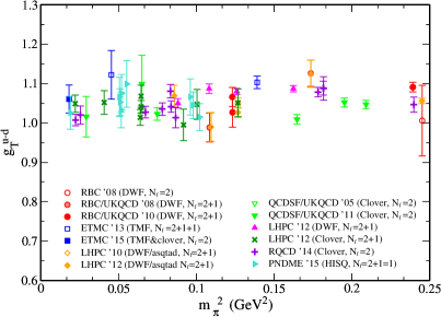
Figure 3: Lattice results for $g_{T}$ as a function of the $m_{\pi}^{2}$, corresponding to: $N_{f}{=}2$ Clover (QCDSF/UKQCD [37, 18, 21]), $N_{f}{=}2$ DWF (RBC [38]), $N_{f}{=}2{+}1$ DWF (RBC/UKQCD [39, 40], LHPC [41]), $N_{f}{=}2{+}1$ DWF on asqtad sea (LHPC [16, 41]), $N_{f}{=}2{+}1$ Clover (LHPC [41]), $N_{f}{=}2{+}1{+}1$ TMF (ETMC [43]), $N_{f}{=}2{+}1{+}1$ HISQ (PNDME [42]), $N_{f}{=}2$ TMF with Clover (ETMC [27]).

The excited states contamination for $g_{T}$ have been also investigated, revealing a weak dependence on the source-sink time separation, $T_{sink}$ [21, 42, 27]: the values from the plateau method do not vary as a function of $T_{sink}$ and are in agreement with the value extracted from the summation method, within statistical uncertainties.

On the experimental side there are available data for $g_{T}$ obtained from combined global analysis of the measured azimuthal asymmetries in SIDIS and in $e^{+}e^{-}\to h_{1}h_{2}X$ (see, e.g. [44]). There are also results from model predictions, for instance the predictions by a covariant quark-diquark model. However, direct comparison of the tensor charges from different models and scales is not always meaningful, since the tensor charges are strongly scale-dependent quantities, in particular at low values of the renormalization scale. Therefore, ab initio calculations of $g_{T}$ from Lattice QCD are extremely useful in providing reliable and model-independent predictions.

4 PDFs on the Lattice

Measurements of parton distribution functions in high-energy processes such as deep-inelastic lepton scattering and Drell-Yan in hadron-hadron collisions are very interesting since they provide information on the quark and gluon structure of a hadron. To leading twist, these quantities give the probability of finding a specific parton in the hadron carrying certain momentum and spin, in the infinite momentum frame. Due to the fact that PDFs are light-cone correlation functions (quark and gluons fields are separated along the light-cone, defined in the real Minkowski time), what is calculated in LQCD are Mellin moments expressed in terms of hadron matrix elements of local operators. Although there is intense activity on the computation of such moments in lattice QCD, it is highly desirable to have information on the PDFs themselves. The Mellin moments are related to the original PDFs through the operator product expansion (OPE). However, the reconstruction of the PDFs appears to be unfeasible since the signal-to-noise ratio becomes very small for higher moments. Also for moments with more than 3 derivatives there is unavoidable mixing with lower dimension operators, which complicates the renormalization procedure. In addition, there is limited progress in calculations of gluon moments (see Section 6), which require a disconnected insertion, has low signal quality and operator mixing.

Recently, a novel direct approach has been proposed by Ji [45], suggesting that one can compute a parton quasi-distribution function, $\tilde{q}(x,\Lambda,P,\Gamma)$, where $x=k/|\vec{P}|$, $\Lambda$ is an ultraviolet cutoff scale, $\vec{P}$ is the momentum of the nucleon, and $\Gamma$ is the Dirac structure of the operator under study. $\tilde{q}(x,\Lambda,P)$ is accessible on the lattice, and for large momenta, one can establish connection with the PDFs through a matching procedure. Such a matching appears in one-loop perturbation theory [46] and the computation of quasi-distribution functions has been carried out in Ref. [47] using $N_{f}{=}2{+}1{+}1$ HISQ gauge ensembles with clover valence quarks, and more recently in Ref [48] for $N_{f}{=}2{+}1{+}1$ twisted mass fermions.

The momentum-dependent non-local static correlation is written as

$$\tilde{q}(x,\Lambda,P_{z},\Gamma)=\int_{-\infty}^{infty}\frac{dz}{4\pi}e^{-izk}\times\left\langle P\right|\bar{\psi}(z)\Gamma e^{ig\int_{0}^{z}A_{z}(z^{\prime})dz^{\prime}}\psi(0)\left|P\right\rangle\,,$$ (10)

where $x$ is the momentum distribution and $e^{ig\int_{0}^{z}A_{z}(z^{\prime})dz^{\prime}}$ is the Wilson line introduced to ensure gauge invariance in the quark distribution. Also, for simplicity, the momentum $\vec{P}$ is taken in the $z$-direction. One of the characteristics of $\tilde{q}$ is that, unlike the case of the physical PDFs, is non=zero for $|x|>1$. When the momentum approached infinity one recovers the physical distribution functions, $q(x,\mu)$, with the infrared region remaining the same. For finite but large enough momenta, $\tilde{q}$ and $q$ are related via

$$q(x,\mu)=q_{bare}(x)\left\{1+\frac{\alpha_{s}}{2\pi}Z_{F}(\mu)\right\}+\frac{\alpha_{s}}{2\pi}\int_{x}^{1}q^{(1)}(x/y,\mu)q_{bare}(y)\frac{dy}{y}+\mathcal{O}(\alpha_{s}^{2})\,,$$ (11)

$$\tilde{q}(x,\Lambda,P_{z})=q_{bare}(x)\left\{1+\frac{\alpha_{s}}{2\pi}\tilde{Z_{F}}(\Lambda,P_{z})\right\}+\frac{\alpha_{s}}{2\pi}\int_{x/x_{c}}^{1}\tilde{q}^{(1)}(x/y,\Lambda,P_{z})q_{bare}(y)\frac{dy}{y}+\mathcal{O}(\alpha_{s}^{2})\,,$$ (12)

where $q_{bare}$ is the bare distribution, $Z_{F}$ and $\tilde{Z}_{F}$ are the wave function corrections, $q^{(1)}$ and $\tilde{q}^{(1)}$ are the vertex corrections. Also, $\mu$ is the renormalization scale and $x_{c}=\Lambda/P_{x}$ is the largest possible value of the momentum distribution, $x$. The leading UV divergences to the quasi-distribution functions are computed in perturbation theory by having $P_{z}$ fixed, while sending $\Lambda\to\infty$. The UV regulator $\Lambda$ will be set to the renormalization scale $\mu$ when relating $\tilde{q}$ at finite momentum to $\tilde{q}$ at infinite momentum.

On the lattice one computes $\tilde{q}(x,\Lambda,P_{z},\Gamma)$ as defined in Eq. (10), which is then used in the lhs of Eq. (12) to calculate the rhs of Eqs. (11) - (12) in order to extract the quark distribution. This makes use of perturbation theory and to date results exist for the non-singlet case and to ${\cal O}(a_{s})$ for the vertex corrections and the self-energy. Thus, a combination of Eqs. (11) - (12) leads to

$$\tilde{q}(x,\Lambda,P_{z}) = q(x,\mu)+\frac{\alpha_{s}}{2\pi}q(x,\mu)\left\{\tilde{Z_{F}}(\Lambda,P_{z})-Z_{F}(\mu)\right\}$$ (13)

$$+ \frac{\alpha_{s}}{2\pi}\int_{x/x_{c}}^{1}\left(\tilde{q}^{(1)}(x/y,\Lambda,P_{z})-q^{(1)}(x/y,\mu)\right)q(y,\mu)\frac{dy}{y}+\mathcal{O}(\alpha_{s}^{2})\,,$$

From the above expression one can isolate $q(x,\mu)$, and by including at the same time anti-quarks ($\bar{q}(x)=-q(-x)$), Eq. (13) can be rewritten as

$$q(x,\mu) = \tilde{q}(x,\Lambda,P_{z})-\frac{\alpha_{s}}{2\pi}\tilde{q}(x,\Lambda,P_{z})\delta\left(\tilde{Z_{F}}(\Lambda,P_{3})-Z_{F}(\mu)\right)$$ (14)

$$-\frac{\alpha_{s}}{2\pi}\int_{-1}^{1}\left(\tilde{q}^{(1)}(\xi,\Lambda,P_{3})-q^{(1)}(\xi,\mu)\right)\tilde{q}(y,\Lambda,P_{z})\frac{dy}{|y|}+\mathcal{O}(\alpha_{s}^{2})\,.$$

A nucleon mass correction in $M_{N}/P_{z}$ can be also made to an arbitrary order. More details are given in Refs. [47, 48].

A first study appeared in Ref [47] for the unpolarized and polarized quasi-distribution functions using clover valence fermions on an $N_{f}{=}2{+}1{+}1$ ensemble of HISQ quarks corresponding to $m_{\pi}\sim$310 MeV. The authors apply HYP smearing to the gauge links, which appears to minimize the discretization effects. In addition, since the multiplicative renormalization of $\tilde{q}$ has not been computed yet, the smearing is important because it shift the renormalization functions close to unity.

For the unpolarized case, the matrix element calculated on the lattice is

$$h(z,\Lambda,P_{z})=\left\langle\vec{P}\right|\bar{\psi}(z)\gamma_{3}\left(\prod_{n}U_{z}(n\hat{z})\right)\psi(0)\left|\vec{P}\right\rangle\,.$$ (15)

Note that, in order to study the polarized operator one should simply substitute the Dirac structure $\gamma_{3}$ with $\gamma_{5}\,\gamma_{3}$. The matrix elements are computed with the nucleon boosted with momentum $P_{z}=\frac{2\pi}{L},\,\frac{4\pi}{L},\,\frac{6\pi}{L}$. In the left panel of Fig. 4 we show results for the isovector $\tilde{q}$ which is the Fourier transformation of $h(z,\Lambda,P_{z})$ in the $z$ coordinate

$$\tilde{q}_{\text{lat}}(x,\Lambda,P_{z})=\int\frac{dz}{4\pi}e^{-izk}h(z,\Lambda,P_{z})\,.$$ (16)

The values for the momentum $P_{z}=\frac{2\pi}{L},\,\frac{4\pi}{L},\,\frac{6\pi}{L}$ are shown with a red, green and cyan color, respectively. One observation is that at momentum $\frac{2\pi}{L}$ the peak of the distribution is centered around $x=1$, where the physical distribution is, in fact, zero. For larger momenta the peak of the band moves towards zero and centered around $x=0.5,\,0.4$ for $P_{z}=\frac{4\pi}{L},\,\frac{6\pi}{L}$, respectively. Also, the value of $\tilde{q}$ at $x=1$ reduces as the momentum increases, which is expected, since for asymptotically large momenta the quasi-distribution functions approach the physical ones. In lattice calculations the maximum momenta are limited by statistical accuracy, and thus, a large-momentum effective field theory should be utilized to relate the finite-momentum $\tilde{q}$ to the physical ones. To do so, one can use perturbative corrections, available to 1-loop level [46]. Due to the fact that the momenta are not infinitely large, the nucleon-mass corrections -expressed in terms of $M_{N}^{2}/(4P_{z}^{2})$- are also important and should taken into account as explained in Ref. [47]. The lattice data for $\tilde{q}$ upon the mass and 1-loop corrections have a milder momentum dependence, and one should finally extrapolate to the infinite momentum limit, using the fit $a+b/P_{z}^{2}$. The extrapolated unpolarized isovector $\tilde{q}$ is shown in the right panel of Fig. 4, where one observes that outside the region $|x|\geq 1$ the curve drops significantly, as expected. The lattice data are plotted with results from global analysis by MSTW [49] and CTEQ-JLab [50], although no attempt for comparison is made since the available lattice data cannot be extrapolated to the chiral limit nor the continuum, and no source of systematics has been addressed.

  

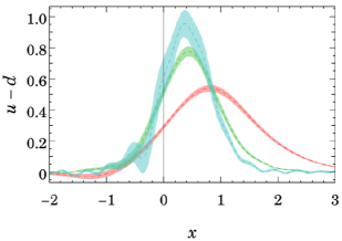
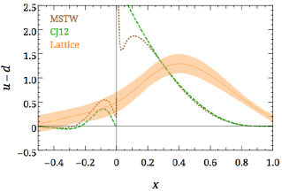
Figure 4: Left: Lattice results for the isovector $\tilde{q}(x)$ using momenta $P_{z}$: $\frac{2\pi}{L}$ (red), $\frac{4\pi}{L}$ (green),$\frac{6\pi}{L}$ (cyan). Right: Unpolarized isovector $\tilde{q}(x)$ upon extrapolation in $P_{z}$ with 68$\%$ C.L (orange band). Brown (green) dotted line corresponds to global analysis of MSTW [49] (CTEQ-JLab [50]).

Another recent study of the unpolarized quasi-distribution function was performed by ETMC, using an ensemble of $N_{f}{=}2{+}1{+}1$ twisted mass fermions at $m_{\pi}\sim 373$MeV. The matrix elements are computed for the 3 lowest momenta: $P_{z}=\frac{2\pi}{L},\,\frac{4\pi}{L},\,\frac{6\pi}{L}$, since the statistical noise does not allow to explore higher momenta. The dependence on the source-sink separation is also studied, showing compatibility within error bars. Two to five HYP smearing steps are applied to the gauge links of the operator, which as mentioned above, it is expected to bring the renormalization function closer to unity. Since the renormalization function for this quantity is not yet available (a perturbative calculation is in progress [51]), a comparison between the unsmeared results with the data from various HYP smearing steps, reveals the influence of the renormalization; it appears that the smearing affect is stronger in the imaginary part. However, the authors of Ref. [48] use the renormalization function of the ultra-local vector current, since for $z=0$, the operator reduces to the local vector current. As a test, one can check the value of the renormalized $h(z=0,\Lambda,P_{z})$, defined in Eq. 15, which is expected to be equal to 1. The authors find for instance that $h^{R}(z=0,\Lambda,4\pi/L)=0.99(3)$.

In the left panel of Fig. 5 we show the isovector $\tilde{q}$ for $P_{z}=\frac{4\pi}{L}$ and 0, 2, 5 HYP smearing steps. As can be seen, the difference between the 0 and 2 steps is more pronounced than the difference of 2 to 5 steps, indicating a saturation of the smearing effect. These data correspond to the 1-loop and nucleon mass corrected results, and both the real and imaginary parts are taken into account. However, the difference between the various HYP steps indicated that the proper renormalization will play an important role, and the renormalized results are expected to agree within statistical errors.

The physical quark distribution function $q$ can be extracted from $\tilde{q}$ and then the mass corrections may be applied. This is shown in the right panel of Fig. 5 for momentum $P_{z}=\frac{6\pi}{L}$. The authors find that while increasing the momentum from $\frac{2\pi}{L}$ to $\frac{6\pi}{L}$, the peak of the $u(x)-d(x)$ moves to smaller values of $x$, for the negative region, the $\bar{d}(x)-\bar{u}(x)$ becomes very small for most of the $x<0$ region. The latter is in qualitative agreement with the behavior of the antiquark distributions as extracted from phenomenological analyses [49, 50, 52]. The nucleon mass corrections lead to a desirable decrease of the distributions in the large $x$ region. Also, the mild oscillatory behavior in the large $x$ region is due to the fact that the Fourier transformation was performed over a finite interval, that is $−L/2\leq z\leq+L/2$.

  

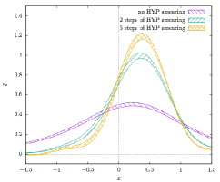
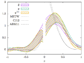
Figure 5: Left: Results for the isovector $\tilde{q}$ upon one-loop and mass corrections for the momentum $P_{z}=4\pi/4$ and for 0, 2 and 5 HYP smearing steps. Right: The quasi-distribution function $\tilde{q}$, the PDF without subtracting the mass correction $q$, and the final PDF, $q(0)$, shown for momentum $P_{z}=\frac{6\pi}{L}$. Various black lines show phenomenological results at 6.25 MeV² from MSTW [49] (CJ12 [50]), ABM11 [52].

5 Nucleon Spin

In 1989 DIS experiments at CERN showed that only a small amount of the proton spin was actually carried by the valence quarks. This was called “the proton spin crisis”, but since then our understanding on the proton spin has evolved. We now know that both the gluons and sea quarks are polarized and, thus, their contribution to the spin is essential. It is also understood that a complete description of the spin requires to take into account the non-perturbative structure of the proton. Using the lattice QCD formalism one can provide significant input towards understanding this open issue. The total nucleon spin is generated by the sum of the quark orbital angular momentum ($L^{q}$), the quark spin ($\Sigma^{q}$) and the gluon angular momentum ($J^{g}$). The quark components are related to $g^{q}_{A}$ and the GFFs of the one-derivative vector at $Q^{2}=0$

$$\frac{1}{2}=\sum_{q}\left(L^{q}+\frac{1}{2}\Delta\Sigma^{q}\right)+J^{g}\,,\quad J^{q}=\frac{1}{2}\left(A_{20}^{q}+B_{20}^{q}\right)\,,\quad L^{q}=J^{q}-\Sigma^{q}\,,\quad\Sigma^{q}=g_{A}^{q}\,,$$ (17)

where $L^{q},\,\Delta\Sigma^{q}$ and $J^{g}$ are gauge invariant. Since we are interested in the individual quark contributions to the various components of the spin, one needs to consider the disconnected contributions.

The computation of disconnected diagrams using improved actions with dynamical fermions became feasible over the last years and for the proper renormalization of the individual quark and isoscalar contributions one should take into account the singlet operator and its proper renormalization (see Ref. [29] for further discussion).

A number of results have appeared recently where the disconnected loop contributions to $g_{A}$ are evaluated as shown in Fig. 6. We observe a nice agreement among results using a number of methods both for the light [9, 11, 53, 54, 55, 56, 57], as well as for the strange quark contributions [8, 9, 11, 10, 54, 55, 56, 57]. For $g_{A}^{light}$ we find $\sim 10\%$ contributions compared to the connected part that must be taken into account in the discussion of the spin carried by quarks in the proton. These contributions are negative and thus reduce the value of $g_{A}^{q}$.

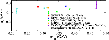
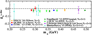
Figure 6: Disconnected contributions for $g_{A}^{q}$ for the light (left) and strange (right) quark contributions.

  

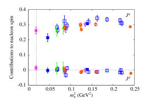
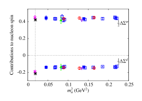
Figure 7: The total spin, $J^{q}$, and the quark spin, $\Sigma^{q}$, carried by the up and down quarks. The lattice data correspond to: $N_{f}{=}2{+}1$ DWF and DWF on asqtad (LHPC [58]), $N_{f}{=}2$ Clover (QCDSF/UKQCD [59]), $N_{f}{=}2$ TMF (ETMC [60]) $N_{f}{=}2{+}1{+}1$ TMF (ETMC [24]) $N_{f}{=}2$ TMF with Clover (ETMC [27]).

In Fig. 7 we show results for the u and d contributions to the total spin, $J^{q}$. It is found that the u-quark exclusively carries the spin attributed to the quarks in the nucleon since $J^{d}$ is consistent with zero for all pion masses and lattice discretization schemes. The quark distribution to the intrinsic spin in also shown in Fig. 7. There is a nice agreement between the results at the physical pion mass using TM fermions [27] and the experimental values for both the u- and the d-quarks. The disconnected contributions have been neglected from most data except for one TMF ensemble at $m_{\pi}=375$ MeV. The effect is shown by the shift of the filled blue square -which ignores disconnected contributions- to the violet triangle -which includes them. Although the effect is small, it is larger than the statistical error and thus one needs to take them into account. The lattice results thus corroborate the missing spin contribution arising from the quarks.

6 Gluon moments of the nucleon

To go further in our understanding for the structure of the nucleon and the missing contributions to its spin we need to consider contribution from the gluonic degrees of freedom. In this section, we will discuss lattice results that predict a sizeable contribution of the gluons to the nucleon spin. Investigation of the gluon distribution functions has also become of high importance in major experimental facilities such as COMPASS and STAR. Experimentally the gluon distributions can be determined from the QCD evolution of the DIS and DIS measurements and a number of groups are carrying out extended analyses.

While the quark moments have been studied extensively [27] there are only a few computations for the gluon moments, mainly due to the bad signal-to-noise ratio, as well as the fact that there is a mixing with the corresponding quark singlet operator. Here we discuss recent results for the unpolarized gluon moment using different methods. This observable can be evaluated by employing the following gluon operator

$${\cal O}_{\mu\nu}^{g}=-{\rm Tr}\left[G_{\mu\rho}G_{\nu\rho}\right],\,$$ (18)

from which one may extract the gluon moment by constructing appropriate combinations of Dirac indices

$$\langle N(p)|{\cal O}^{L}_{b}|N(p)\rangle=\left(m_{N}+\frac{2}{3\,E_{N}}\vec{p}^{2}\right)\,\langle x\rangle_{g}\,,\quad{\cal O}^{L}_{b}\equiv{\cal O}^{L}_{44}-\frac{1}{3}\sum_{j=1}^{3}{\cal O}^{L}_{jj}.\,$$ (19)

The lattice discretization of the gluon operator is denoted by ${\cal O}^{L}_{b}$ and can be expressed in terms of plaquettes

$${\cal O}^{L}_{b}=\frac{4}{9}\frac{\beta}{a}\sum_{x}\left(\sum_{i}\mbox{tr}_{c}[U_{i4}(x,t)]-\sum_{i<j}\mbox{tr}_{c}[U_{ij}(x,t)]\right)\,.$$ (20)

The advantage of this operator is that the gluon moment, $\langle x\rangle_{g}$, can be extracted directly from lattice data at zero momentum transfer, as can be seen from the rhs of Eq. (19). However, the fact that terms of similar magnitude are subtracted leads potentially to a noisy signal.

A direct computation of the gluon moment is related to the following ratio at zero momentum transfer

$$\frac{\left\langle[N(t)N(0)]_{p=0}\mathcal{B}(\tau)\right\rangle}{\langle N(t)N(0)_{p=0}\rangle}\stackrel{{\scriptstyle 0\ll\tau\ll t}}{{=}}m_{N}\langle x\rangle_{g}\,,$$ (21)

which comprises of disconnected diagrams only. The three-point function can, thus, be written as a product of nucleon two-point functions and the gluon operator. Although disconnected contributions are notoriously difficult and noisy, applying smearing to the gauge links in the gluon operator improves the quality of the signal. This was demonstrated in Ref. [61] using $N_{f}{=}2+1+1$ twisted mass fermions at $m_{\pi}\sim 373$ MeV. The authors test both HYP and stout smearings and find a significant reduction of the noise-to-signal ratios after five steps for the HYP smearing, and ten steps for the stout smearing.

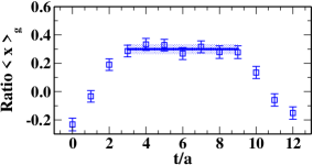
Figure 8: The ratio for $\langle x\rangle_{g}$ for $N_{f}{=}2+1+1$ twisted mass fermions at $m_{\pi}\sim 375$ MeV after 10 iterations of stout smearing steps.

An example is shown in Fig. 8 for the ratio leading to $\langle x\rangle_{g}$ after 10 iterations of stout smearing steps. A challenge with such a computation is that to obtain physical results for $\langle x\rangle_{g}$, the lattice matrix element needs to be renormalized. Since the gluon operator is singlet it mixes with the quark momentum fraction $\langle x\rangle_{q}$, as well as with other operators that are: (a) gauge invariant, or (b) BRS-variations, or (c) vanish by the equations of motion. However, in physical matrix elements the mixing with the operators (a)-(c) vanishes and the mixing reduces to a $2\times 2$ matrix, that is

$$\left(\begin{array}[]{c}\langle x\rangle_{g}^{\overline{\rm MS}}(\mu)\\ \sum_{q}\langle x\rangle_{q}^{\overline{\rm MS}}(\mu)\\ \end{array}\right)=\left(\begin{array}[]{cc}Z_{gg}^{\overline{\rm MS}}(\mu)&Z_{gq}^{\overline{\rm MS}}(\mu)\\ Z_{qg}^{\overline{\rm MS}}(\mu)&Z_{qq}^{\overline{\rm MS}}(\mu)\\ \end{array}\right)\,\left(\begin{array}[]{c}\langle x\rangle_{g}\\ \sum_{q}\langle x\rangle_{q}\\ \end{array}\right)\,,$$ (28)

where $\mu$ is the renormalization scale, usually set to 2 GeV. Note that, in the quenched approximation the mixing matrix simplifies considerably since both $Z_{gq}$ and $Z_{qg}$ become $1-Z_{qq}$ and $1-Z_{gg}$, respectively. For the renormalization of $\langle x\rangle_{g}$ the relevant matrix elements are $Z_{gg}$ and $Z_{qq}$ and the relation to the bare quark and gluon moments is

$$\langle x\rangle_{g}^{\overline{\rm MS}}=Z_{gg}^{\overline{\rm MS}}\langle x\rangle_{g}+Z_{gq}^{\overline{\rm MS}}\sum_{q}\langle x\rangle_{q}\,.$$ (29)

Due to the mixing and the involvement of disconnected contributions, an appropriate renormalization scheme to extract the multiplicative renormalization functions and the mixing coefficients non-perturbatively is a difficult task. As a first step we thus use perturbation theory to compute the elements of the mixing matrix. One of the advantages of the perturbative calculation [62] is that the results can be computed directly in the $\overline{\rm MS}$ scheme without an intermediate RI-type step. Since the gauge links of the operator are smeared for signal improvement, an equivalent procedure is also followed in the perturbative calculation in order to match the non-perturbative calculation of $\langle x\rangle_{g}$. In the calculation of Ref. [63] the preferred smearing is stout since it is analytically defined in both the perturbative and non-perturbative evaluations. Note, however, that in the perturbative computation of the renormalization functions introduction of smearing increases the number of algebraic expression, which explodes as the stout smearing steps increase. Currently, the computation is performed to 2 smearing steps, which already involved millions of terms. The smearing parameter is chosen to be small, and thus, more levels of smearing is expected to bring in a very small effect, due to the polynomial dependence on the smearing parameter. For the work of Ref. [63] the renormalized matrix element at $m_{\pi}=373$ MeV in the $\overline{\rm MS}$ at 2 GeV is found to be: $\langle x\rangle_{g}=0.309(25)$.

An alternative approach to extract the matrix elements of the gluon operator utilizes the Euclidean form of the Feynman-Hellman theorem. In this methodology an operator $\lambda{\cal O}$ is introduced into the total QCD action, and the matrix element of the operator can be extracted from the derivative of the energy of the state with respect to $\lambda$

$$\frac{\partial E_{N}(\lambda)}{\partial\lambda}=(:\frac{\partial\hat{S}(\lambda)}{\partial\lambda}:)_{N(p)N(p),\lambda}\,,$$ (30)

where $:...:$ denotes the subtraction of the vacuum expectation value of the operator. By combining the above equations with the continuum decomposition expression, one can extract the gluon moment at zero momentum transfer

$$\langle x\rangle_{g}=\frac{2}{3m_{N}}\frac{\partial m_{N}}{\partial\lambda}{\big{|}_{\lambda=0}}\,.$$ (31)

Note that the Feynman-Hellman methodology requires production of new gauge ensembles for each value of the $\lambda$ parameter (and each operator), which is computationally costly, especially for $m_{\pi}$ close to the physical value. This methodology was applied in Ref. [64] in the quenched approximation for clover fermions at ensembles corresponding to several values of $m_{\pi}$ so that the extrapolation to the chiral limit can be taken, as shown in Fig. 9. The extrapolated value is $\langle x\rangle_{g}=0.43(7)(5)$, which, despite being quenched, it is close to the value of ETMC using dynamical twisted mass fermions [63].

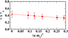
Figure 9: $\langle x\rangle_{g}$ for $N_{f}{=}0$ clover fermions [64] as a functions of the pion mass squared, $(a\,m_{\pi})^{2}$. The open circle corresponds to the chirally extrapolated result.

A different direction for the computation of not only the gluon, but also the quark moments relies on a complete gauge-invariant decomposition of the nucleon spin (see Eq. (17)) in terms of the quark spin, the quark orbital angular momentum, and the glue angular momentum operators, as defined from the symmetric energy-momentum tensor. Thus, instead of computing directly $J_{q}$ and $J_{g}$ from the explicit definitions

$$\vec{J}_{q}=\frac{1}{2}\vec{\Sigma}_{q}+\vec{L}_{q}=\int d^{3}x\,\bigg{[}\frac{1}{2}\,\overline{\psi}\,\vec{\gamma}\,\gamma^{5}\,\psi+\psi^{\dagger}\,\{\vec{x}\times(i\vec{D})\}\,\psi\bigg{]}\,,\quad\vec{J}_{g}=\int d^{3}x\,\bigg{[}\vec{x}\times(\vec{E}\times\vec{B})\bigg{]}\,,$$ (32)

one can calculate them from the energy-momentum tensor

$$J_{q,g}^{i}=\frac{1}{2}\,\epsilon^{ijk}\,\int\,d^{3}x\,\left(\mathcal{T}_{q,g}^{0k}\,x^{j}-\mathcal{T}_{q,g}^{0j}\,x^{k}\right)\,,$$ (33)

which in Euclidean space the quark and gluon operators are

$${\mathcal{T}}_{\{4i\}q}^{(E)} = (-1)\,\frac{i}{4}\displaystyle\sum_{f}\overline{\psi}_{f}\left[\gamma_{4}\stackrel{{\scriptstyle\rightarrow}}{{D}}_{i}+\gamma_{i}\stackrel{{\scriptstyle\rightarrow}}{{D}}_{4}-\gamma_{4}\stackrel{{\scriptstyle\leftarrow}}{{D}}_{i}-\gamma_{i}\stackrel{{\scriptstyle\leftarrow}}{{D}}_{4}\right]\psi_{f},$$ (34)

$${\mathcal{T}}_{\{4i\}g}^{(E)} = (+i)\,\bigg{[}-\frac{1}{2}\displaystyle\sum_{k=1}^{3}2\,\mbox{Tr}^{\mbox{\scriptsize color}}\left[G_{4k}\,G_{ki}+G_{ik}\,G_{k4}\right]\bigg{]}.$$ (35)

The complete calculation of the quark and glue momenta and angular momenta on a quenched lattice for Wilson fermions has been presented in Ref. [65], including both connected and disconnected insertions for the quark contributions. Three ensembles have been employed with $m_{\pi}=$478, 538, 650 MeV. The overlap operator is used for the gauge field tensor, which leads to less noisy results than that from usual gauge links. Details on the computation can be found in Ref. [65]. Regarding the renormalization of the operators, the authors use sum rules to define renormalization conditions on the lattice. This results from the fact that although the momentum and angular momentum fractions of the quark and glue are renormalization scale and scheme dependent individually, their sums are not because the nucleon total momentum and angular momentum are conserved. One thus obtains

$$J_{q,g}+\frac{1}{2}Z_{q,g}^{L}\left[T_{1}(0)+T_{2}(0)\right]_{q,g}\,,\quad\langle x\rangle_{q,g}=Z_{q,g}^{L}T_{1}(0)_{q,g}\,,$$ (36)

and

$$\langle x\rangle_{q}+\langle x\rangle_{g}\,=\,Z_{q}^{L}T_{1}(0)_{q}+Z_{g}^{L}T_{1}(0)_{g} = 1\,,$$ (37)

$$J_{q}+J_{g}\,=\,\frac{1}{2}\,\bigg{\{}Z_{q}^{L}\left[T_{1}(0)+T_{2}(0)\right]_{q}+Z_{g}^{L}\left[T_{1}(0)+T_{2}(0)\right]_{g}\bigg{\}} = \frac{1}{2}\,,$$ (38)

which also leads to

$$Z_{q}^{L}T_{2}(0)_{q}+Z_{g}^{L}T_{2}(0)_{g}=0\,,$$ (39)

providing sufficient conditions and cross-checks to obtain the renormalization functions.

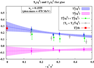
Figure 10: $T_{1}$, $T_{2}$ for gluons and angular momentum $J_{g}$ using quenched Wilson fermions [65].

In Fig. 10 we show results for the gluon contributions corresponding to 478 MeV. The extrapolated value for the gluon unpolarized moment is $\langle x\rangle_{g}=0.313(56)$, which is compatible with the results presented above for both quenched [64] and dynamical fermions [63].

7 Neutron Electric Dipole Moment

There is recently a major activity in LQCD computation of the neutron electric dipole moment (EDM), $\vec{d}_{N}$, which we review in this section. A non-zero EDM indicates the violation of parity ($P$) and time ($T$) symmetries, and consequently of $CP$, probing physics BSM [66]. So far, no finite neutron EDM (nEDM) has been reported and current bounds are still several orders of magnitude below what one expects from $CP$-violation induced by weak interactions. Several experiments are under way to improve the upper bound on the nEDM value, with the best experimental upper limit being [67, 68, 69]

$$|\vec{d}_{N}|<2.9\times 10^{-13}e\cdot{\rm fm}\ (90\%\ {\rm CL})\,.$$ (40)

To investigate theoretically a finite nEDM, we add to the $CP$-conserving QCD Lagrangian density a $CP$-violating interaction term, proportional to the topological charge, $q$

$${\cal L}_{\rm QCD}\left(x\right)=\frac{1}{2g^{2}}{\rm Tr}\left[G_{\mu\nu}\left(x\right)G_{\mu\nu}\left(x\right)\right]+\sum_{f}{\overline{\psi}}_{f}\left(x\right)(\gamma_{\mu}D_{\mu}+m_{f})\psi_{f}\left(x\right)\,-i\theta q\left(x\right)\,,$$ (41)

$$q\left(x\right)=\frac{1}{32\pi^{2}}\epsilon_{\mu\nu\rho\sigma}{\rm Tr}\left[G_{\mu\nu}\left(x\right)G_{\rho\sigma}\left(x\right)\right]\,,\hskip 85.35826pt$$ (42)

where $\psi_{f}$ denotes a fermion field of flavor $f$ with bare mass $m_{f}$ and $G_{\mu\nu}$ is the gluon field tensor. The so called $\theta$-parameter controls the strength of the $CP$-breaking, and the addition of the $CP$-violating term leads to a non-zero value for nEDM. The $\theta$-parameter can be taken as a small continuous parameter allowing a perturbative expansion and only keep first order contributions in $\theta$. This is in accordance to effective field theory calculations (see references within [71]) that give a bound of the order $\theta\lesssim{\cal O}\left(10^{-10}-10^{-11}\right)$.

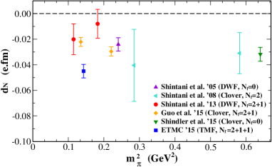
Figure 11: The nEDM versus $m_{\pi}^{2}$ for: a) $N_{f}{=}2{+}1{+}1$ twisted mass fermions [71] (blue square) corresponding to a weighted average using different methods for extracting $F_{3}(0)$), b) $N_{f}{=}0$ DWF [72] (magenta upward triangles), $N_{f}{=}2{+}1$ DWF [76] (red circles) and $N_{f}{=}0$ clover fermions [77] (green downward triangles) by extracting the $CP$-odd $F_{3}(Q^{2})$ and fitting its $Q^{2}$-dependence, c) $N_{f}{=}2$ Clover fermions [75] (turquoise left triangles) obtained using a background electric field, d) $N_{f}{=}2{+}1$ clover fermions [74] (orange diamonds) by implementing an imaginary $\theta$.

The quantity, which is of interest is the nEDM, $\vec{d}_{N}$, which at leading order of $\theta$ and in momentum space is given by [70]

$$|\vec{d}_{N}|=\theta\lim_{Q^{2}\to 0}\frac{|F_{3}(Q^{2})|}{2m_{N}}\,,$$ (43)

where $m_{N}$ denotes the mass of the neutron, $Q^{2}{=}-q^{2}$ the four-momentum transfer in Euclidean space ($q{=}p_{f}-p_{i}$) and $F_{3}(Q^{2})$ is the $CP$-odd form factor. In a theory with $CP$ violation we can, therefore, calculate the electric dipole moment by evaluating the zero momentum transfer limit of the $CP$-odd form factor. However, the $CP$-violating matrix element gives access to $Q_{k}F_{3}(Q^{2})$ and not to $F_{3}(Q^{2})$ alone, hindering a direct evaluation of $F_{3}(0)$. Details on different methods for the extraction of $F_{3}(Q^{2})$ can be found in Ref. [71].

Besides extracting the nEDM from the $CP$-odd form factor [72, 76, 77, 71], there are alternative methods to compute the nEDM, such are the implementation of an imaginary $\theta$ [74], or with an application of an external electric field and measuring the associated energy shifts [75]. A collection of lattice results are displayed in Fig. 11, using different methods for obtaining $d_{N}$, as well as, different definition of the topological charge. We note that the results of Ref. [77] have been extrapolated to the continuum limit.

8 Summary and Challenges

Lattice QCD has entered a new era in terms of simulations with the light quark masses fixed to their physical value. This is due to major improvements in algorithm and techniques coupled with increase in the computational power. However, many challenges lie ahead: development of appropriate algorithms to reduce the statistical errors at reduced cost and addressing systematic uncertainties in order to compute accurately observables that reproduce experimental data or can probe beyond the standard model physics.

For hadron structure, simulations at different lattice spacings and larger volumes are crucial for a proper study of lattice artifacts in order to provide reliable results at the continuum limit. Such studies require an accuracy, which is difficult to achieve with standard methods. Noise reduction techniques are, thus, essential in order to settle some of the long-standing discrepancies reviewed in this talk. Similarly techniques developed for the computation of disconnected quark loop diagrams, such as the truncated solver method [78] need to be improved since they become inefficient at the physical point [57]. Thus, new ideas will be needed to compute disconnected contributions to hadron structure to an accuracy of a few percent. Utilization of new computer architectures such as GPUs has proved essential for the evaluation of disconnected diagrams and this is a direction that we will further pursue in the future.

Other open issues such as the nucleon spin need the evaluation of quantities that are challenging to compute, such as gluonic contributions. As discussed in this review, there are several challenges in the computation of the gluon moments, including increased gauge noise and mixing with other operators. Perturbation theory has been utilized in order to successfully compute the multiplicative renormalization and disentangle the operator mixing.

Evaluation of the nucleon matrix elements for the electromagnetic current in a theory with a $CP$-violating term in the Lagrangian, yields the value of the neutron electric dipole moment from first principles. Despite its difficulties, such a calculation can guide planned experiments.

Despite the challenges of LQCD calculations, simulations at the physical point have eliminated one of the systematic uncertainties that was inherent in all lattice calculations in the past, that is the difficulty to quantify systematic error due to the chiral extrapolation. Calculating observables directly at the physical point holds the promise of resolving discrepancies on benchmark quantities like $g_{A}$ and reliably compute quantities relevant for revealing possible new physics BSM.

Acknowledgments: I would like to thank the organizers for their invitation to participate and for providing partial financial support. I also want to thank my collaborators for fruitful discussions.

References

- [1] A. Antognini, et al. [CREMA Collaboration], Science 339 (2013) 417.
- [2] C. Carlson, Prog. Part. Nucl. Phys. 82, 59 (2015), [arXiv:1502.05314].
- [3] P. Mohr, B. Taylor, D. Newell, Rev. Mod. Phys. 84, 1527 (2012), [arXiv:1203.5425].
- [4] R. Pohl et al., Nature 466 (2010) 213.
- [5] M. Constantinou et al. [ETM Collaboration], JHEP 1008, 068 (2010), [arXiv:1004.1115].
- [6] M. Constantinou, R. Horsley, H. Panagopoulos, H. Perlt, P. Rakow, G. Schierholz, A. Schiller, J. Zanotti, Phys. Rev. D 91, no. 1, 014502 (2015), [arXiv:1408.6047].
- [7] C. Alexandrou, M. Constantinou, H. Panagopoulos [ETM Collaboration], arXiv:1509.00213.
- [8] R. Babich, R. Brower, M. Clark, G. Fleming, J. Osborn, C. Rebbi, D. Schaich, Phys. Rev. D 85, 054510 (2012), [arXiv:1012.0562].
- [9] G. Bali et al. [QCDSF Collaboration], Phys. Rev. Lett. 108, 222001 (2012), [arXiv:1112.3354].
- [10] M. Engelhardt, Phys. Rev. D 86, 114510 (2012), [arXiv:1210.0025].
- [11] A. Abdel-Rehim, C. Alexandrou, M. Constantinou, V. Drach, K. Hadjiyiannakou, K. Jansen, G. Koutsou, A. Vaquero, Phys. Rev. D 89, 034501 (2014), [arXiv:1310.6339].
- [12] T. Yamazaki, Y. Aoki, T. Blum, H.W. Lin, M.F. Lin, S. Ohta, S. Sasaki, R. Tweedie, J. Zanotti [RBC/UKQCD Collaboration], Phys. Rev. Lett. 100, 171602 (2008), [arXiv:0801.4016].
- [13] T. Yamazaki, Y. Aoki, T. Blum, H.W. Lin, S. Ohta, S. Sasaki, R. Tweedie, J. Zanotti, Phys. Rev. D 79, 114505 (2009), [arXiv:0904.2039].
- [14] S. Ohta [RBC/UKQCD Collaboration], PoS LATTICE 2013 274 (2013), [arXiv:1309.7942].
- [15] Y.B. Yang, Y. Chen, T. Draper, M. Gong, K.F Liu, Z. Liu, J.P. Ma [QCD Collaboration], PoS(LATTICE2014)137, [arXiv:1411.0927].
- [16] J. Bratt et al. [LHP Collaboration], Phys. Rev. D 82, 094502 (2010), [arXiv:1001.3620].
- [17] C. Alexandrou, M. Brinet, J. Carbonell, M. Constantinou, P. Harraud, P. Guichon, K. Jansen, T. Korzec, M. Papinutto [ETM Collaboration], Phys. Rev. D 83, 045010 (2011), [arXiv:1012.0857].
- [18] D. Pleiter et al. [QCDSF/UKQCD Collaboration], PoS(LATT2010), 153 (2010), [arXiv:1101.2326].
- [19] S. Capitani, M. Della Morte, G. von Hippel, B. Jager, A. Juttner, B. Knippschild, H. Meyer, H. Wittig, Phys. Rev. D 86, 074502 (2012), [arXiv:1205.0180].
- [20] R. Horsley, Y. Nakamura, A. Nobile, P. Rakow, G. Schierholz , J. Zanotti, Phys. Lett. B 732, 41 (2014), [arXiv:1302.2233].
- [21] G. Bali, S. Collins, B. Glässle, M. Göckeler, J. Najjar, R. Rödl, A. Schäfer, R. Schiel, W. Söldner, A. Sternbeck , Phys. Rev. D 91, no. 5, 054501 (2015), [arXiv:1412.7336].
- [22] J. Green, M. Engelhardt, S. Krieg, J. Negele, A. Pochinsky, S. Syritsyn, PoS LATTICE 2012, 170 (2012), [arXiv:1211.0253].
- [23] B. J. Owen, J. Dragos, W. Kamleh, D. Leinweber, M. Mahbub, B. Menadue, J. Zanotti, Phys. Lett. B 723, 217 (2013), [arXiv:1212.4668].
- [24] C. Alexandrou, M. Constantinou, S. Dinter, V. Drach, K. Jansen, C. Kallidonis, G. Koutsou, Phys. Rev. D 88, 014509 (2013), [arXiv:1303.5979].
- [25] T. Bhattacharya, S. Cohen, R. Gupta, A. Joseph, H. W. Lin, B. Yoon, Phys. Rev. D 89, 094502 (2014), [arXiv:1306.5435].
- [26] R. Gupta, T. Bhattacharya, A. Joseph, H.W. Lin, B. Yoon [PNDME Collaboration], PoS(LATTICE2014)152, [arXiv:1501.07639].
- [27] A. Abdel-Rehim et al., arXiv:1507.04936.
- [28] J. Beringer et al., Particle Data Group, Phys. Rev. D 86, 010001 (2012).
- [29] M. Constantinou, PoS(LATTICE2014)001 (2015), [arXiv:1411.0078].
- [30] H. Abele, M. Astruc Hoffmann, S. Baessler, D. Dubbers, F. Gluck, U. Muller, V. Nesvizhevsky, J. Reich, O. Zimmer, Phys. Rev. Lett. 88, 211801 (2002), [hep-ex/0206058].
- [31] J. Nico, J. Phys. G 36, 104001 (2009).
- [32] A. Young et al., J. Phys. G 41, no. 11, 114007 (2014).
- [33] S. Baeßler, J. Bowman, S. Penttilä, D. Počanić, J. Phys. G 41, 114003 (2014), [arXiv:1408.4737].
- [34] T. Bhattacharya, V. Cirigliano, S. Cohen, A. Filipuzzi, M. Gonzalez-Alonso, M. Graesser, R. Gupta, H. W. Lin, Phys. Rev. D 85, 054512 (2012), [arXiv:1110.6448].
- [35] H. Gao et al., Eur. Phys. J. Plus 126, 2 (2011), [arXiv:1009.3803].
- [36] J. Ellis, K. Olive, arXiv:1001.3651.
- [37] M. Gockeler, P. Hagler, R. Horsley, D. Pleiter, P. Rakow, A. Schafer, G. Schierholz, J. Zanotti [QCDSF and UKQCD Collaborations], Phys. Lett. B 627, 113 (2005), [hep-lat/0507001].
- [38] H. W. Lin, T. Blum, S. Ohta, S. Sasaki, T. Yamazaki, Phys. Rev. D 78, 014505 (2008), [arXiv:0802.0863].
- [39] S. Ohta, T. Yamazaki [RBC and UKQCD Collaborations], arXiv:0810.0045.
- [40] Y. Aoki, T. Blum, H. W. Lin, S. Ohta, S. Sasaki, R. Tweedie, J. Zanotti, T. Yamazaki, Phys. Rev. D 82, 014501 (2010), [arXiv:1003.3387].
- [41] J. R. Green, J. W. Negele, A. V. Pochinsky, S. N. Syritsyn, M. Engelhardt, S. Krieg, Phys. Rev. D 86, 114509 (2012), [arXiv:1206.4527].
- [42] T. Bhattacharya, V. Cirigliano, S. Cohen, R. Gupta, A. Joseph, H. W. Lin, B. Yoon, arXiv:1506.06411.
- [43] C. Alexandrou, M. Constantinou, K. Jansen, G. Koutsou, H. Panagopoulos, PoS LATTICE 2013, 294 (2014), [arXiv:1311.4670].
- [44] M. Anselmino, M. Boglione, U. D’Alesio, S. Melis, F. Murgia A. Prokudin, Phys. Rev. D 87, 094019 (2013), [arXiv:1303.3822].
- [45] X. Ji, Phys. Rev. Lett. 110, 262002 (2013), [arXiv:1305.1539].
- [46] X. Xiong, X. Ji, J. Zhang, Y. Zhao, Phys. Rev. D 90, no. 1, 014051 (2014), [arXiv:1310.7471].
- [47] H. W. Lin, J. Chen, S. Cohen, X. Ji, Phys. Rev. D 91, 054510 (2015), [arXiv:1402.1462].
- [48] C. Alexandrou, K. Cichy, V. Drach, E. Garcia-Ramos, K. Hadjiyiannakou, K. Jansen, F. Steffens, C. Wiese, Phys. Rev. D 92, no. 1, 014502 (2015), [arXiv:1504.07455].
- [49] A. Martin, W. Stirling, R. Thorne, G. Watt, Eur. Phys. J. C 63, 189 (2009), [arXiv:0901.0002].
- [50] J. Owens, A. Accardi, W. Melnitchouk, Phys. Rev. D 87, no. 9, 094012 (2013), [arXiv:1212.1702].
- [51] M. Constantinou, H. Panagopoulos, Perturbative renormalization of quasi-distribution functions in Lattice QCD.
- [52] S. Alekhin, J. Blumlein, S. Moch, Phys. Rev. D 86, 054009 (2012), [arXiv:1202.2281].
- [53] Y.B. Yang, M. Gong, K.F. Liu, M. Sun [QCD Collaboration], PoS(LATTICE2014)138, [arXiv:1504.04052].
- [54] S. Meinel et al. [LHP Collaboration], PoS(LATTICE2014)139.
- [55] A. Chambers et al. [CSSM/QCDSF/UKQCD Collaboration], PoS(LATTICE2014)165, [arXiv:1412.6569].
- [56] T. Bhattacharya, R. Gupta, B. Yoon, PoS LATTICE 2014, 141 (2014), [arXiv:1503.05975].
- [57] C. Alexandrou, M. Constantinou, V. Drach, K. Hadjiyiannakou, K. Jansen G. Koutsou, A. Vaquero [ETM Collaboration], PoS(LATTICE2014)140, [arXiv:1410.8761].
- [58] S. Syritsyn, J. Green, J. Negele, A. Pochinsky, M. Engelhardt, P. Hagler, B. Musch, W. Schroers, PoS LATTICE 2011, 178 (2011), [arXiv:1111.0718].
- [59] A. Sternbeck et al., PoS LATTICE 2011, 177 (2011), [arXiv:1203.6579].
- [60] C. Alexandrou, J. Carbonell, M. Constantinou, P. Harraud, P. Guichon, K. Jansen, C. Kallidonis, T. Korzec, M. Papinutto, Phys. Rev. D 83, 114513 (2011), [arXiv:1104.1600].
- [61] C. Alexandrou, V. Drach, K. Hadjiyiannakou, K. Jansen, B. Kostrzewa, C. Wiese, PoS LATTICE 2013, 289 (2014), [arXiv:1311.3174].
- [62] M. Constantinou, H. Panagopoulos, in preparation.
- [63] C. Alexandrou, M. Constantinou, V. Drach, K. Hadjiyiannakou, K. Jansen, B. Kostrzewa, H. Panagopoulos, C. Wiese, in preparation.
- [64] R. Horsley, R. Millo, Y. Nakamura, H. Perlt, D. Pleiter, P. Rakow, G. Schierholz, A. Schiller, F. Winter, J. Zanotti [QCDSF/UKQCD Collaborations], Phys. Lett. B 714, 312 (2012), [arXiv:1205.6410].
- [65] M. Deka et al., Phys. Rev. D 91, no. 1, 014505 (2015), [arXiv:1312.4816].
- [66] M. Pospelov, A. Ritz, Annals Phys. 318, 119 (2005), [hep-ph/0504231].
- [67] V. Helaine [nEDM Collaboration], EPJ Web Conf. 73 (2014) 07003.
- [68] C. Baker et al., Phys. Rev. Lett. 97, 131801 (2006), [hep-ex/0602020].
- [69] C. Baker et al., Phys. Rev. Lett. 98, 149102 (2007), [arXiv:0704.1354].
- [70] S. Barr, W. Marciano in “CP Violation”, ed. C Jarlskog (World Scientific, Singapore, 1988).
- [71] C. Alexandrou, A. Athenodorou, M. Constantinou, K. Hadjiyiannakou, K. Jansen, G. Koutsou, K. Ottnad, M. Petschlies, arXiv:1510.05823.
- [72] E. Shintani, S. Aoki, N. Ishizuka, K. Kanaya, Y. Kikukawa, Y. Kuramashi, M. Okawa, Y. Tanigchi, A. Ukawa, T. Yoshie, Phys. Rev. D 72, 014504 (2005), [hep-lat/0505022].
- [73] E. Shintani S. Aoki, N. Ishizuka, K. Kanaya, Y. Kikukawa, Y. Kuramashi, M. Okawa, A. Ukawa, T. Yoshie, Phys. Rev. D 75, 034507 (2007), [hep-lat/0611032].
- [74] F. Guo, R. Horsley, U. Meissner, Y. Nakamura, H. Perlt, P. Rakow, G. Schierholz, A. Schiller, J. Zanotti, Phys. Rev. Lett. 115, no. 6, 062001 (2015), [arXiv:1502.02295].
- [75] E. Shintani, S. Aoki, Y. Kuramashi, Phys. Rev. D 78, 014503 (2008), [arXiv:0803.0797].
- [76] E. Shintani, T. Blum, A. Soni, T. Izubuchi, PoS LATTICE 2013, 298 (2014).
- [77] A. Shindler, T. Luu, J. de Vries, arXiv:1507.02343.
- [78] G. Bali, S. Collins, A. Schäfer, Comput. Phys. Commun. 181, 1570 (2010), [arXiv:0910.3970].