Intermittency at Fine Scales and Complex Singularities of Turbulent Couette Flow

Abstract

Fine scales of turbulent velocity fields, beyond the inertial range and well into the dissipative range, are highly intermittent. It has been hypothesized that complex plane singularities are the principal mechanism behind fine scale intermittency. In this article, we view the velocity field of a turbulent flow as an analytic function of time. Although the function is only available for real values of time, we present a numerical technique to analytically continue the function to complex values of time, and with sufficient fidelity to locate and visualize the singularity closest to the real axis. Using this technique, we demonstrate a robust connection between temporal intermittency and the location of singularities in the complex plane.

Department of Mathematics, University of Michigan (sandre/divakar@umich.edu).

1 Introduction

Intermittency in turbulent flows refers to sharp and spatially isolated peaks of energy contained in large wave numbers, beyond the inertial range and well into the dissipative range. In the words of Batchelor and Townsend [2], who discovered this phenomenon, “the energy associated with large wave-numbers is very unevenly distributed in space” and “there appear to be isolated regions in which the large wave-numbers are ’activated’, separated by regions of comparative quiescence.” This fine scale intermittency is a fundamental feature of turbulent flows [1, 5, 17].

Frisch and Morf [7] hypothesized that intermittency is a manifestation of singularities in the complex plane. Thus the activation mechanism is believed to be the occurrence of singularities in the complex plane, with the intermittent peak occurring right below the singularity closest to the real axis. Complex singularities are intrinsically easier to study with a single independent variable. Therefore Frisch and Morf shifted the emphasis to temporal intermittency, with time as the single independent variable with the entire velocity field viewed as a function of time.

The connection between intermittency and complex singularities has been demonstrated in a variety of systems such as Langevin’s and Burger’s equations [7, 15]. However, to the best of the authors’ knowledge, such a connection is yet to be demonstrated for the incompressible Navier-Stokes equations in the turbulent regime. In this article, we develop a numerical technique that is applicable to trajectories of large scale PDE. Using that technique, we demonstrate a robust connection between temporal intermittency and complex singularities.

Here at the outset, we reprise a beautiful argument of Kraichnan [12]. The argument is heuristic but gives powerful intuition regarding the phenomenon of fine scale intermittency, partially explaining many of the plots found later in this article and showing why the manifestation of intermittency is clearest in the dissipative range. The argument is as follows. Suppose that the velocity field of the turbulent flow is infinitely differentiable with each derivative being square integrable. Direct numerical simulation of turbulence from the incompressible Navier-Stokes equations implicitly assumes the velocity field to be analytic, and the great success of direct numerical simulation is certainly evidence for the validity of that assumption. The assumption of smoothness implies that energy should fall off faster than algebraically (and exponentially fast if the velocity field is analytic) with increase in wave-number. The super-algebraic and possibly exponential decay of energy with wave-number means that a change in wave-number “by a few percent” implies an “enormous” change in the energy associated with the wave-number. If the energy spectra is governed by a length scale that varies gently from region to region, this gentle variation is enormously amplified and shows up as intermittency in the high wave-numbers. In essence, the hypothesis of Frisch and Morf [7], investigated and validated in this article, is that the gentle variation in the large which gets amplified into intermittency in fine scales is due to singularities in the complex plane.

Energy dissipation per unit mass, denoted $\epsilon$, is an important parameter in turbulence. Indeed, it is the only parameter in the Kolmogorov theory of the inertial range [1]. Fine scale intermittency may be detected experimentally through an analysis of the variation in $\epsilon$ [13, 14]. Thus physical space analysis of turbulent velocity fields obtained from numerical simulation suffices for demonstration of spatial intermittency as well as for isolating structures associated with that phenomenon [16].

The tack we take in this article is different, and possibly complementary. We study fine scale intermittency through analytic continuation into the complex $t$-plane. An advantage is a direct connection to the hypothesized mechanism. Continuation into the complex $t$-plane could be complementary to physical space analysis as we discuss in the concluding section.

Analytic continuation into the complex plane is infamous for its numerical difficulty. The technique of Padé approximation, and strategies for better numerical stability, have been set forth by Weideman [25], Gonnet, Pachón, and Trefethen [8] and Webb [22]. A crucial ingredient is the use of complex phase plots championed by Wegert and others [23, 24], and whose pertinence to the computation of complex singularities was communicated to us in person by Hrothgar and Trefethen. These phase plots play a central role in our technique and we rely on them to locate singularities in the complex plane. The phase plots proved to be a more viable approach to stabilize numerical computations than strategies for deflating tiny and repeated singular values developed in [8].

All numerical simulations are carried out with constant time steps for reasons explained in section 2. The numerical method for locating complex singularities described in section 2 interpolates to Chebyshev points of the second kind from equi-spaced data. The Chebyshev series are filtered before computing Padé approximants. Many of the ingredients in the numerical method we describe have occurred in earlier work in some form. Our contribution is to synthesize a numerical method that works robustly for turbulent flows.

Somewhat counter-intuitively, the high dimensionality of discretizations of turbulent velocity fields appears to be a help rather than a hindrance. The numerical method of section 2 takes advantage of intermittency in high wave-numbers in locating the complex singularities.

In section 3, we compute the complex singularities of six periodic or relative periodic solutions of plane Couette flow. The plane Couette flow set-up we use is the minimal flow unit [10]. The minimal flow unit was derived by constraining turbulent Couette flow into a small box at the low Reynolds number of $Re=400$. Since the Reynolds number is low, the dissipative range is reached easily. Another advantage of the minimal flow unit is its connection to the self-sustaining process developed by Waleffe [21]. While inertial range turbulence is statistical, turbulence is also characterized by coherent structures. The self-sustaining process emphasizes the dynamical aspects of fine-scale turbulence with connections to coherent structures.

The six periodic and relative periodic orbits, whose complex singularities are computed, are from earlier work [19] . For each of these orbits, we demonstrate a clear connection between intermittency and the location of complex singularities. There are no profound advantages to using periodic orbits. One could use any turbulent trajectory. But as a practical matter there are two reasons for opting for these solutions of plane Couette flow. Firstly, the orbits are reported in [19] with estimates for their precision so that they may be reproduced. Secondly, the earlier study of these orbits has identified different regimes enabling a preliminary investigation of the connection between observed turbulence and the location of complex singularities.

The concluding section 4 discusses further connections of the work presented in this article. One of these is to the spatial analysis of fine scale intermittency, already alluded to above. Another is to blow-ups in physical space.

2 Numerical method

The numerical method used for computing singularities will be described using the Lorenz example. The Lorenz equations $\dot{x}=10(y-x),\,\dot{y}=28x-y-xz,\>\dot{z}=-8z/3+xy$ admit singular solutions that may be expanded in convergent psi-series as follows [20]:

$$x(t) = \frac{P_{-1}(\eta)}{t-t_{0}}+P_{0}(\eta)+P_{1}(\eta)(t-t_{0})+P_{2}(\eta)(t-t_{0})^{2}+\cdots$$

$$y(t) =\frac{Q_{-2}(\eta)}{(t-t_{0})^{2}}+ \frac{Q_{-1}(\eta)}{t-t_{0}}+Q_{0}(\eta)+Q_{1}(\eta)(t-t_{0})+Q_{2}(\eta)(t-t_{0})^{2}+\cdots$$

$$z(t) =\frac{R_{-2}(\eta)}{(t-t_{0})^{2}}+ \frac{R_{-1}(\eta)}{t-t_{0}}+R_{0}(\eta)+R_{1}(\eta)(t-t_{0})+R_{2}(\eta)(t-t_{0})^{2}+\cdots$$ (2.1)

Here $\eta=\log(t-t_{0})$ with the branch cut chosen appropriately, and $P_{i},Q_{i},R_{i}$ are polynomials in $\eta$. These polynomials are given explicitly in earlier work [20]. Here we note that $Q_{-2}=-i/5$, $R_{-2}=1/5$, $P_{-1}=Q_{-1}=2i$, and $R_{-1}=17/9$, so that the dominant part of the singularity is a pole for $x(t)$ and a double pole for $y(t)$ and $z(t)$. The first terms in the psi-series which are not constants are

$$Q_{-1}=-{\frac{349}{81}}\,i-{\frac{988}{81}}\,i(\eta+C),\>\>R_{-1}={\frac{1385}{54}}-{\frac{988}{81}}\,(\eta+C),$$

where $C$ is an undetermined constant. There is another undetermined constant $D$ in the psi-series which occurs for the first time in $Q_{2}$.

Not all the singularities of Lorenz are proved to be psi-series of this form. However, a few singularities were examined numerically in [20] and were all found to be psi-series of the form given above. In addition, the locations of the singularities were determined with $10$ digits of precision, which makes the Lorenz example useful for validating the numerical method described here.

The Lorenz example, being of only $3$ dimensions, can be tackled using a number of techniques. It is amenable to extended precision computations. Orbits of the Lorenz system were computed with $500$ digits of accuracy in [20]. For the incompressible Navier-Stokes equations in the fully turbulent regime, simply integrating the trajectories is among the most complex and difficult computations. The room for deploying techniques that find complex plane singularities is much more limited.

In this section, we refine Padé based techniques [8, 25] and derive a numerical method that is reliable when applied to turbulent signals. The numerical method is described in three stages. The first stage is an analysis in the purely real time domain. The second stage is the computation of a Padé approximant. The third stage is a discussion of the Wegert–style phase plots of the Padé approximant. Complex singularities are located using phase plots, and we compare the locations obtained through the phase plots to the far more accurate computations of [20].

2.1 Chebyshev series and its analysis

To describe the numerical method, we look at the $z$-coordinate of the $AABB$ orbit of the Lorenz system. For the nomenclature of Lorenz orbits, see [18]. The $AABB$ orbit has period equal to $3.084276...$

The Lorenz orbits can be computed using a special method described in [18]. Turbulence trajectories are obtained using ordinary direct numerical simulation, and to obtain a reliable comparison the Lorenz orbits too were computed using numerical integration. There is one important point pertinent to direct numerical simulation, however. The time-steps must be constant.

If a Hamiltonian system is integrated using constant time-steps and a symplectic discretization, it has been proved that the numerical trajectory (ignoring rounding errors) approximates the trajectory of a perturbed Hamiltonian with error that is exponentially small in the time-step for an interval of time that is exponentially long in the time-step [9]. The arguments of [9] can be made to apply to non-Hamiltonian ordinary differential equations without major modifications. Thus if the time-step is constant, there is reason to think that the effect of the discretization error is to introduce a smooth and analytic perturbation of the underlying differential equation. On the other hand, adaptive time-stepping strategies are non-smooth, and even though they allow for longer time-steps, they destroy the analytic structure of the underlying differential equation.

Once a signal $u(i\Delta t)$ is obtained for integer values of $i$, the next step is to pick a time interval and compute a Chebyshev series. Suppose that the time interval is $[a,b]$ with $a=i_{a}\Delta t$ and $b=i_{b}\Delta t$. To convert, the signal $u(t)$, $a\leq t\leq b$, into a Chebyshev series, we first interpolate the signal at Chebyshev points (of the second kind) $\cos(j\pi/n)$, $j=0,1,\ldots,n$, shifted for the interval $[-1,1]$ to the interval $[a,b]$. If $t_{j}$ is a shifted Chebyshev point in $[a,b]$ and $t_{j}\in[i\Delta t,(i+1)\Delta t]$, the value of $u(t_{j})$ is computed through polynomial interpolation using the nodes $t=\left(i-k\right)\Delta t,\,(i-k+1)\Delta t,\ldots,(i+k+1)\Delta t$.

The polynomial interpolation is from equi-spaced data. However, there is no need to fear the Runge phenomenon as $t_{j}$ is near the center of the domain of interpolation. In addition, $k$ is small, with $k=4$ in almost all reported computations ($k=4$ implies at least $8$-th order accuracy). The interpolation was carried using the barycentric Lagrange formula, which is known to have excellent numerical stability [3]. Interpolated Chebyshev data was moved back to the original equi-spaced grid to assess the quality of interpolation, and to ensure that no information was lost during interpolation.

Once the signal $u(t)$ is available at Chebyshev points shifted to the interval $[a,b]$, it is converted to a Chebyshev series using the discrete cosine transform. If $T_{k}(x)=\frac{1}{2}\left(z^{k}+\frac{1}{z^{k}}\right)$ denotes the Chebyshev polynomial of degree $n$, with $z$ determined from $x=\frac{1}{2}\left(z+\frac{1}{z}\right)$, and $\tilde{T}_{k}$ is $T_{k}$ shifted from the interval $[-1,1]$ to the interval $[a,b]$, the Chebyshev series obtained from the discrete cosine transform is of the form

$$u(t)=c_{0}+c_{1}\tilde{T}_{1}(t)+c_{2}\tilde{T}_{2}+\cdots+c_{n}\tilde{T}_{n}$$

and is valid for $a\leq t\leq b$. This Chebyshev series will be converted into a Padé approximant later. It is important to do a preliminary analysis of the coefficients $c_{i}$ before computing the Padé approximant. Much of the analysis is visual as we will now explain.

Figure 2.1: Plots of the $z$-coordinate of the $AABB$ Lorenz orbit. The top plots show $z$ as a function of time, with the dots being interpolants at Chebyshev points. The bottom plots are $|c_{n}|$, absolute values of coefficients of the Chebyshev series, of the top plots graphed against $n$.

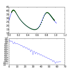
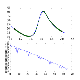
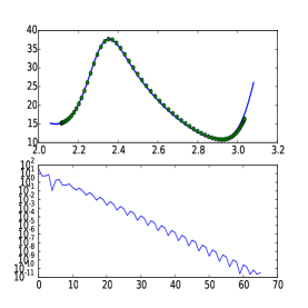
Figure 2.1 shows plots for the Lorenz orbit $AABB$. The period of the orbit has been split into three equal segments. It is easily noticeable that the Chebyshev series of the middle segment is cleaner with a more pronounced pattern. The Chebyshev coefficients decrease exponentially all three segments, but in the middle segment we see spikes that protrude down with a clear rhythm. Isolating a Chebyshev series with this kind of pattern is crucial. The Padé approximant relies on this kind of a pattern to locate the complex singularity. If the pattern is not clear to begin with the Padé approximant will not work too well.

For some of the Lorenz orbits and even turbulent orbits of plane Couette flow, we are able to find Chebyshev series that exhibit patterns that are even cleaner and more pronounced than the middle segment in Figure 2.1. For others, the pattern is not as clean. In addition to the pattern being clean and well-established, it is advantageous if the pattern starts early.

Figure 2.2: Filtered signal corresponding to the middle segment of Figure 2.1 and a linear fit of its Chebyshev coefficients.

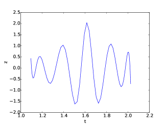
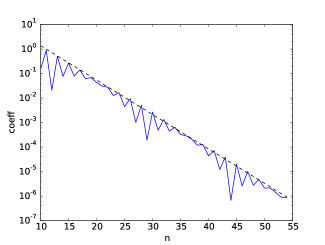
Once a Chebyshev series with a clean pattern has been isolated, the pattern can be improved further using filtering as shown in Figure 2.2. Here the Chebyshev series of the middle segment was filtered by setting to zero the first $10$ coefficients, since they are not part of a pattern, as well as the last few which were deemed to be not sufficiently accurate. The filtered signal on the left side of Figure 2.2 almost gives away the real part of the location of the singularity as $\Re(t)\approx 1.6$. Filtering makes the intermittency more pronounced.

Identification of the role of filtering in accentuating intermittency is due to Frisch and co-workers [7, 15]. As noted by those authors, the roots of the idea are found in the theory of complex variables as developed in the late 1800s and early 1900s. In that body of work, the asymptotics of the coefficients of a power series are connected to the form and location of the singularities. The further out one goes into the series, the clearer the asymptotics will be. In numerical work, however, one cannot go too far because of accuracy issues.

Alternatively, the role of filtering may be understood as follows. Suppose that $f(t)$ is analytic except for singularities at $t=a\pm ib$, with $b\neq 0$, in the complex plane. Let $t_{0}\in\mathbb{R}$. Consider the expansion of $f(t)$ in powers of $(t-t_{0})$ with $t_{0}$ varying along the real line. The radius of convergence is least at $t_{0}=a$ and the coefficient of $(t-t_{0})^{n}$ spikes at $t_{0}=a$, for large $n$. The increase in steepness of the spike at $t_{0}=a$ (in a relative sense) as $n$ increases is the substance of the argument for the connection between intermittency and complex singularities. In this setting, it is quite clear that we can add a polynomial or any entire function to $f(t)$ without moving the singularity. Such an addition can destroy intermittency in the coefficients of $(t-t_{0})^{n}$ for small $n$, but the intermittency will show up for larger $n$. Thus intermittency may be identified more clearly in the signal $f(t)$ if the coefficients of $(t-t_{0})^{n}$ for certain small $n$ are filtered out. In the numerical method we are describing, the range of filtering is determined by examining the coefficients of the Chebyshev series.

The right hand plot in Figure 2.2 shows a linear fit of the filtered Chebyshev coefficients. The linear fit is obtained as follows. An index $i$ is selected if and only if it is in the range that survives filtering ($10<i<55$ in Figure 2.2) and $|c_{i}|>|c_{j}|$ for $j>i$. The linear fit of $\log|c_{i}|$ vs $i$ is computed using only the selected indices $i$. The linear fit approximates the outer envelope of $\log|c_{i}|$ vs $i$ as shown in Figure 2.2. If the slope of the fit is $\rho$,

$$\Re(t)=\frac{1}{2}\left(\rho+\frac{1}{\rho}\right)\cos\theta,\>\>\Im(t)=\frac{1}{2}\left(\rho-\frac{1}{\rho}\right)\sin\theta$$ (2.2)

is an ellipse in the complex plane parametrized by $\theta$. Standard results in complex function theory imply that there must be a singularity on this ellipse. The Padé approximant is far more reliable inside the ellipse than outside it, as we will momentarily see.

2.2 Computation of Padé approximant

Given a Chebyshev series, its Padé approximant

$$\sum_{i=0}^{n}c_{i}T_{i}(t)\approx\frac{a_{0}+a_{1}T_{1}(t)+\cdots+a_{p}T_{p}(t)}{b_{0}+b_{1}T_{1}+\cdots+b_{q}T_{q}(t)}$$

is computed using

$$\left(c_{0}+c_{1}T_{1}+\cdots+c_{n}T_{n}\right)\left(b_{0}+b_{1}T_{1}+\cdots+b_{q}T_{q}\right)-\left(a_{0}+a_{1}T_{1}+\cdots+a_{p}T_{p}\right)\approx 0.$$

If Chebyshev polynomials are multiplied using the identity $T_{i}T_{j}=\frac{1}{2}\left(T_{i+j}+T_{|i-j|}\right)$ and coefficients are equated to zero, we get a set of $n+1$ linear relations between the unknown coefficients $a_{i}$ and $b_{i}$.

We follow Gonnet, Pachón, and Trefethen [8] in using the singular value decomposition of the last $(n-p)$ of the equations to solve for the $b_{i}$ with the normalization $\sum|b_{i}|^{2}=1$. The same authors recommend strategies to reduce the degree of the dominator if the singular values are too small or if the smallest singular values are repeated. We have experimented with these strategies, but rely on different criteria to obtain robust Padé approximants. Removing small singular values was problematic and threw away too much information. In fact, in most of our computations we prefer to have denominators of large degree with the degree being nearly $200$ in some cases.

Figure 2.3: Comparison of filtered coefficients of Figure 2.2 with coefficients of the Padé approximation. The Padé approximations are dotted.

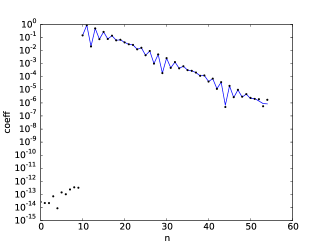
Figure 2.3 compares the filtered coefficients and the Chebyshev coefficients of the Padé approximation. The Padé approximation was obtained using $p=15$ and $q=25$. Since the first $10$ coefficients are filtered out, the first $10$ coefficients in the numerator are $0$. Most of the fitting is taking place in the denominator. Close observation shows that the Padé approximation gets the pattern near the tail slightly differently. However, the quality of the approximation is excellent through the range of the Chebyshev coefficients. Obtaining a high quality approximation of this sort is essential.

If two analytic functions agree exactly for $t\in[a,b]$, they will agree everywhere in the complex plane. If one of those two functions is a polynomial, it is incapable of picking up singularities of the other function, even if the agreement over $t\in[a,b]$ is very close, because polynomials are entire functions. The hope with Padé approximations is that they will pick up the singularity in the complex plane because they are rational in $t$. For that to be true, we need close agreement over $t\in[a,b]$ at a minimum. In fact, such close agreement also appears to be sufficient if the original signal is properly filtered.

2.3 Phase plots

As mentioned above, the left side plot in Figure 2.2 gives a good indication of $\Re(t_{0})$ if $t_{0}$ is the location of the singularity. The imaginary part $\Im(t_{0})$ may be obtained by plotting the Padé approximant for complex values of $t$. Phase plots [23, 24] of a complex function $f(z)$ depict the function by indicating the phase $\arg f(z)$ using a color code. Such plots reveal a wealth of information about poles and zeros. According to Wegert and Semmler [24], the precise origin of the idea of phase plots is difficult to determine.

Figure 2.4: Phase plots of Padé approximants of the $z$ and $x$ coordinates, respectively, of the Lorenz orbit $AABB$ corresponding to the middle segment in Figure 2.1. The colors code for the phase or argument at a point in the complex $t$-plane.

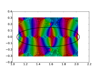
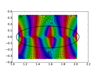
Figure 2.4 shows phase plots for the $z$ (left side) and $x$ (right side) coordinates of the middle segment of the Lorenz orbit $AABB$. Each of the $11$ zeros of the filtered signal shown in Figure 2.2 may be easily located in the phase plot on the left. At a zero the colors red-blue-green rotate in a counter-clockwise sense (opposite of Wegert’s convention). The ellipses shown as thick lines correspond to (2.2).

The phase plot also picks up a singularity near the boundary of the ellipse and with $\Re(t)\approx 1.6$ in both the plots. In the left hand plot, corresponding to $z(t)$, the Padé approximant appears to be attempting to pick up a double pole. The colors outside the ellipse are not as reliable as those inside. Yet one may see that the Padé approximant is attempting two clockwise rotations of the colors red-blue-green. In the right hand plot, corresponding to $x(t)$, there is clearly a single pole at the same location. The double pole in the $z(t)$ phase plot is attempting to pick up the dominant part in the psi-series (2.1), which is a double pole for $z(t)$. Similarly, the phase plot for $x(t)$ is picking a single pole because the dominant part in the psi-series is a single pole. In both cases, the artifacts of Padé approximation are well outside the ellipse.

Orbit	$x$	$y$	$z$	accurate
$AB$	$0.175$	$0.176$	$0.172$	$0.1714501006$
$AAB$	$0.170$	$0.167$	$0.169$	$0.1617621257$
$AAAB$	$0.162$	$0.158$	$0.150$	$0.1563426260$
$AABB$	$0.170$	$0.170$	$0.156$	$0.1636066901$

Table 2.1: Imaginary parts of the singularities closest to the real $t$-axis for four Lorenz orbits. The $x,y,z$ columns are from singularity locations determined using the $x,y,z$ coordinates, respectively. The final column is from extended precision computations [20].

Table 2.1 furthers validates the numerical method by comparing the complex singularity location determined using $x$, $y$, and $z$ coordinates with a more accurate computation from earlier work. It appears that the singularity location is determined correctly with about two digits of precision. Since the method for determining the singularity is graphical, and based on mouse-clicks, two digits of precision is about as much as we expect.

We have avoided finding roots of the polynomial in the denominator of the Padé approximant. Polynomial root finding is often numerically unsound. For the Lorenz orbits, denominator degrees range from $25$ to $40$. For the Couette orbits that we next turn to, the denominator degrees can be larger than $100$ and polynomial root-finding is infeasible. The phase plots are more reliable and informative.

3 Application to plane Couette flow

Orbit	$Re_{\tau}$	$L$	$M$	$N$	$dx^{+}$	$dy^{+}$	$dz^{+}$
P1	$28$	$32$	$64$	$48$	$4.9$	$1.4$	$2.2$
P2	$33$	$48$	$64$	$48$	$3.8$	$1.6$	$2.6$
P3	$33$	$64$	$56$	$48$	$2.9$	$1.9$	$2.6$
P4	$33$	$48$	$64$	$48$	$3.8$	$1.6$	$2.6$
P5	$34$	$48$	$64$	$48$	$3.9$	$1.7$	$2.7$
P6	$34$	$48$	$64$	$48$	$3.9$	$1.7$	$2.7$

Table 3.1: Grid resolution data for $6$ periodic or relative periodic solutions of plane Couette flow.

The velocity field of plane Couette flow is represented as

$${\bf u}(x,y,z,t)=\sum_{\ell=-L/2}^{L/2}\sum_{n=-N/2}^{N/2}\sum_{m=0}^{M}{\bf u}_{l,m,n}(t)\exp\left(\frac{i\ell x}{\Lambda_{x}}+\frac{inz}{\Lambda_{z}}\right)T_{m}(y).$$

Thus the velocity field is periodic in $x$ and $z$ with periods equal to $2\pi\Lambda_{x}$ and $2\pi\Lambda_{z}$. For the minimal flow unit, these periods are $5.4977..$ and $3.7699...$, respectively [10]. As before, $T_{m}$ are Chebyshev polynomials. At the walls $y=\pm 1$, the velocity field satisfies the boundary condition ${\bf u}=(\pm 1,0,0)$. For the minimal flow unit, the Reynolds number in the incompressible Navier-Stokes equations

$$\frac{\partial{\bf u}}{\partial t}+({\bf u}.\nabla){\bf u}=-\nabla p+\frac{1}{Re}\triangle{\bf u}$$

is $Re=400$. The pressure $p$ is determined by the incompressibility constraint $\nabla.{\bf u}=0$.

Table 3.1 shows resolution data for six periodic or relative periodic solutions of the minimal flow unit. A more detailed description of these orbits may be found in [19]. The orbits are labeled P1 through P6. P1 was first computed by Kawahara and Kida [11].

The frictional Reynolds number $Re_{\tau}$ of all six orbits is low, although they exhibit some features of turbulence such as a sharp peak in turbulence energy production in the near wall region. The orbits capture other aspects of buffer layer dynamics as well [19]. The purpose of the minimal flow unit is to capture certain essential features of turbulence in as small a system as possible. The fact that the Reynolds number is low, makes it easier to reach into the high wave-number region where intermittency manifests itself most clearly.

Table 3.1 gives the spacing between grid points in the $x,y,z$ direction in frictional units. For the non-uniform Chebyshev grid in the $y$-direction, the reported number is the maximum spacing. There is no question that all six orbits are exceedingly well-resolved. Good resolution is essential for reaching wave-numbers where intermittency is pronounced.

The Lorenz system is only $3$ dimensional. For the minimal flow unit, the dimensionality of the spatial discretizations we use is more than $10^{5}$. Since the numerical method of the previous section is visual, only a small fraction of these modes can be examined. We examine about $50$ modes for each orbit. These modes are indexed by $k$. Let $\delta\ell=L/64$, $\delta m=M/32$, and $\delta n=N/64$. For $0\leq k\mod 16<6$ and $k=15$, these modes are $\ell,\,m,\,n\approx 1+j\delta\ell,\,1+j\delta m,\,1+j\delta n$, where $j=k\mod 16$. For $6\leq k\mod 16<12$, we use $\ell=m=n=j-5$, where $j=k\mod 16$ as before. For $12\leq k\mod 16<15$, we use $\ell,\,m,\,n=L/4+(j-14),\,M/2+(j-14),\,N/4+(j-14)$, where $j=k\mod 16$ as before.

If ${\bf u}=(u,v,w)$, we extract the stream-wise $u$ mode if $0\leq k<16$, the wall-normal $v$ mode if $16\leq k<32$, and the span-wise $w$ mode if $32\leq k<48$. Most of these modes are complex valued, and we retain only the real part in the signal that is extracted.

The selection of modes for $0\leq k<48$ is admittedly a little arbitrary. The aim is to look at a few low wave-numbers, a few in the middle, and a few higher wave-numbers. The choice of wave-numbers proved adequate for demonstrating the connection between intermittency and complex singularities in all six orbits.

Orbit	$k$	$n_{fst}$	$n_{lst}$	$p$	$q$	$d$
P1	$19$	$12$	$65$	$18$	$45$	$12.0$
P2	$24$	$50$	$200$	$98$	$100$	$4.3$
P3	$7$	$45$	$140$	$68$	$70$	$5.5$
P4	$0$	$200$	$400$	$218$	$180$	$2.6$
P5	$10$	$75$	$250$	$98$	$150$	$3.8$
P6	$1$	$100$	$250$	$123$	$125$	$4.3$

Table 3.2: Data for singularity computations. The $k$ column gives the mode for which the Chebyshev series in time had the best pattern. The interpretation of $k$ is found in the text. All Chebyshev modes $c_{i}$ outside of $(n_{fst},n_{lst}]$ were filtered out. The $p$ and $q$ columns give the degrees of the Padé numerator and denominator, respectively. Notice that most of the coefficients in the numerator are nearly zero because of filtering. The last column gives the estimated distance of the singularity from the real $t$-axis.

Figure 3.1: The filtered Chebyshev series for P1, P2, P3, and P5 (clockwise from top-left). The $y$-axis is the absolute value of the Chebyshev coefficient of $T_{n}(t)$. The circular markers are approximations computed using the Padé approximant.

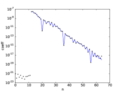
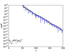
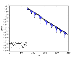
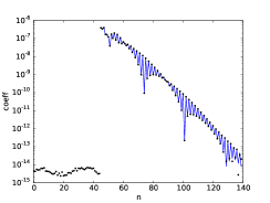
Table 3.2 shows the parameters used for computing the complex singularities. The mode $k$ and the filtering interval are chosen so that the coefficients of Chebyshev series in time exhibit a clean pattern. Plots of the filtered series are shown in Figure 3.1 for P1, P2, P3, and P5. In each case, a clear pattern is discernible, and the Padé approximants reproduce the coefficients with excellent accuracy.

The plots in Figure 3.1 pick modes corresponding to values of $k$ listed in Table 3.2. We tried to pick the $k$ for which the pattern in the Chebyshev series was the cleanest. Although there are other choices of $k$ that are nearly as good, a pattern shows up cleanly only for a few values of $k$.

The need to select $k$ carefully may be explained as follows. In complex function theory, $f(z)$ is usually a complex valued function of a complex variable. However, much of complex function theory goes through with little change even if $f(z)$ takes values in a Hilbert space or a Banach space, as long as $z$ is a complex variable. For instance, Cauchy’s theorem continues to be true.

We may think of ${\bf u}(t)$, the velocity field, as an analytic function of $t$ which takes values in some Hilbert space, although the velocity field is computed only for real values of $t$. The singularity at a point $t_{0}$ in the complex $t$-plane may be thought of as a series of some type in $(t-t_{0})$, something like the psi-series in (2.1), with coefficients in a Hilbert space.

When we pick a mode corresponding to some $k$ and record the variation of that mode in time, we are essentially taking an inner product of the mode and the expansion of the singularity. The Padé approximant tries to pick up the dominant part of the singularity. Two random vectors in high dimensional space are nearly orthogonal. Ordinarily the dominant part of the singularity does not project well when an inner-product is taken. Thus the need to pick $k$ carefully.

3.1 Intermittency and singularities in the complex $t$-plane

Figure 3.2: An intermittent high-wavenumber signal as a function of time and a phase plot of the Padé approximant after filtering for some other mode (the mode corresponding to $k$ listed in Table 3.2) for the orbits P1, P2, P4, and P6 (clockwise from top left).

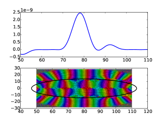
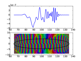
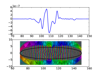
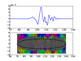
The connection between complex singularities and intermittency for solutions of the minimal flow unit is demonstrated in Figure 3.2. For each of the four orbits shown, the top plot is an intermittent high wave-number signal that was not filtered. The mode that was chosen corresponds to $k$ with $12\leq k\mod 16<16$, with the interpretation of $k$ given above. Almost any $k$ in this range can be picked.

All the phase plots, except for P1, are clean inside the ellipse. For P4 and P5, there is a singularity near the boundary of the ellipse, corresponding to the intermittency, but no spurious singularities are found inside the ellipse. The intermittency in P2 is not as pronounced and there may be more one singularity near the border of the ellipse. The filtered signals corresponding to the phase plots are not shown. Yet the oscillation of these signals with $t$ for real $t$ is clear from the phase plots. When interpreting the phase plots, it must be borne in mind that a counter-clockwise cycle of red-blue-green is a zero, while a clockwise cycle is a pole.

Following [7, 12], the reason that intermittency manifests itself in the high wave-numbers, without filtering, but is more pronounced only after filtering in the lower wave-numbers may be explained as follows. The energy in the spatial modes of the velocity field decreases exponentially with wave-number in the dissipative range. At a given point in time, with $t$ real, this rate is related in some way to the distance to the nearest singularity in the complex $t$-plane. The rate appears to be highest right below the singularity. A small change in the rate causes a much bigger change in the relative magnitude of the energy in the high wave-numbers, making intermittency quite pronounced as evident from Figure 3.2.

3.2 Distance of the singularities from the real axis

We do not claim much accuracy for the distances of the singularities from the real $t$-axis reported in Table 3.2. The errors may be as high as $20$%. Nevertheless, it is very clear that P1’s singularity is much farther way than that of P2 through P6.

Within the confines of the minimal flow unit, P2 through P6 are all in the turbulent regime. However, P1 is intermediate between laminar flow and turbulent flow [11, 19]. The laminar solution of course is constant in time and therefore an entire function. P1’s singularity seems to be much farther out because it is intermediate between laminar flow and turbulent flow.

Another question we may ask is about the type of the singularities. Are they poles of some order, or are they approximable by a pole of some order? For Lorenz, we know that the psi-series are convergent singular solutions. Although not all singularities are proved to be of that form, a few singularities have been analyzed in extended precision and verified to be psi-series [20]. The dominant part in the psi-series is either a pole or a double pole. Thus the success of Padé is not a big surprise.

In the case of the incompressible Navier-Stokes equations, the analytic form of singular solutions is not known. The Padé approximants use poles to approximate all kinds of singularities and do not give direct information about the form of the singularities. Yet the clarity with which Padé approximants locate the singularities, as shown by the phase plots of Figure 3.2, makes us think that the form of the singularities is unlikely to be much more complex than for Lorenz.

Another related question is about the number of singularities. Each of the orbits P1 through P6 seems to be governed by a single dominant singularity, or a tight cluster of singularities closest to the real axis in the case of P2. For a long trajectory and in the complex $t$-plane as a whole, it appears reasonable to suspect that singularities are numerous and occur with increasing density as the Reynolds number increases.

4 Discussion

Computations described in the previous section, even though limited to the minimal flow unit of plane Couette turbulence, offer definite evidence that intermittency in fine scales is due to singularities in the complex plane as suspected by Frisch and others [5, 7].

All our computations of complex singularities are in the time domain. However, intermittency also has a significant spatial aspect [17]. The connection between singularities in the time domain and spatial aspects of intermittency is not entirely clear. It may be possible to combine spatial modes in a manner that the temporal intermittency becomes particularly pronounced.

On the other hand, the velocity field at a fixed value of time may have singularities if the spatial coordinates are allowed to be complex. It is unclear what such spatial singularities look like and how they relate to temporal singularities.

All six orbits discussed in the previous section go through one cycle of the self-sustaining process in a single period [19]. The self-sustaining process as developed by Waleffe [21] is characterized in the spatial domain in terms of rolls and streaks. Each of the six orbits of the minimal flow unit is governed by a single dominant singularity (and its complex conjugate), or perhaps by a tight cluster of singularities. The possibility of a connection between the self-sustaining process and the location of singularities in the complex $t$-plane may be worth investigating.

The finite time blow-up problem for the incompressible Navier-Stokes equations has been viewed in light of complex singularities [4, 6]. The robustness with which complex singularities are located and visualized in Figure 3.2 suggests that computing the distance of the singularities from the real $t$-axis as a function of the Reynolds number may shed some light on this topic. However, there is a subtle difference between mathematical and computational investigations of finite time blow-up.

The evidence that direct numerical simulation algorithms solve the Navier-Stokes equations is overwhelming. Yet there is a subtle difference between numerical and mathematical investigations. In mathematical formulations, the velocity field of the Navier-Stokes equations is allowed to belong to certain function spaces, and these function spaces are much wider than the class of velocity fields that are subject to numerical simulation. Any direct numerical simulation code will become unstable if the initial velocity fields are not sufficiently regular. At high Reynolds numbers such as $Re_{\tau}=1000$, establishing a turbulent initial state can pose far greater difficulties than sustaining turbulence. In fact, at such Reynolds numbers, attempting to transition to turbulence by adding a small disturbance to laminar flow is nearly impossible because of the large number of transitional instabilities. A turbulent initial condition is established by slowly raising the Reynolds number. Thus turbulent velocity fields are pre-selected in a way to induce statistical steadiness in the flow with respect to time integration.

5 Acknowledgements

We are very thankful to Nick Trefethen, and his students Hrothgar and Marcus Webb, for sharing their work on Padé approximation with us. This research was partially supported by NSF grant DMS-1115277.

References

- [1] G.K. Batchelor. The Theory of Homogeneous Turbulence. Cambridge University Press, 1953.
- [2] G.K. Batchelor and A.A. Townsend. The nature of turbulent motion at large wave-numbers. Proceedings of the Royal Society of London, Series A, 199:238–255, 1949.
- [3] J.-P. Berrut and L.N. Trefethen. Barycentric Lagrange interpolation. SIAM Review, 46:501–517, 2004.
- [4] A. Biswas and C. Foias. On the maximal space analyticity radius for the 3d Navier-Stokes equations and energy cascades. Annali di Matematica, 193:739–777, 2014.
- [5] U. Frisch. Turbulence. Cambridge University Press, 1995.
- [6] U. Frisch, T. Matsumoto, and J. Bec. Singularities of the Euler flow? not out of the blue! Journal of Statistical Physics, 113:761–781, 2003.
- [7] U. Frisch and R. Morf. Intermittency in nonlinear dynamics and singularities at complex times. Physical Review A, 23:2673–2705, 1981.
- [8] P. Gonnet, R. Pachon, and L.N. Trefethen. Robust rational interpolation and least squares. Electronic Transactions on Numerical Analysis, 38:146–167, 2011.
- [9] E. Hairer and C. Lubich. The lifespan of backward error analysis for numerical integrators. Numerische Mathematik, 76:441–462, 1997.
- [10] J.M. Hamilton, J. Kim, and F. Waleffe. Regeneration mechanisms of near-wall turbulence structures. Journal of Fluid Mechanics, 287:317–348, 1995.
- [11] G. Kawahara and S. Kida. Periodic motion embedded in plane Couette turbulence: regeneration cycle and burst. Journal of Fluid Mechanics, 449:291–300, 2001.
- [12] R.H. Kraichnan. Intermittency in the very small scales of turbulence. Physics of Fluids, 10:2080–2083, 1967.
- [13] C. Meneveau and K.R. Sreenivasan. Simple multifractal cascade model for fully developed turbulence. Physical Review Letters, 59:1424–1427, 1987.
- [14] C. Meneveau and K.R. Sreenivasan. The multifractal nature of turbulent energy dissipation. Journal of Fluid Mechanics, 224:429–484, 1991.
- [15] W. Pauls and U. Frisch. A Borel transform method for locating singularities of Taylor and Fourier series. Journal of Statistical Physics, 127:1095–1119, 2007.
- [16] J. Schumacher, K.R. Sreenivasan, and P.K. Yeung. Very fine structures in scalar mixing. Journal of Fluid Mechanics, 531:113–122, 2005.
- [17] K.R. Sreenivasan. Fractals and multifractals in fluid turbulence. Annu. Rev. Fluid Mech., 23:539–600, 1991.
- [18] D. Viswanath. Symbolic dynamics and periodic orbits of the Lorenz attractor. Nonlinearity, 16:1035–1056, 2003.
- [19] D. Viswanath. Recurrent motions within plane Couette turbulence. Journal of Fluid Mechanics, 580:339–358, 2007.
- [20] D. Viswanath and S. Şahutoğlu. Complex singularities and the Lorenz attractor. SIAM Review, 52:294–314, 2010.
- [21] F. Waleffe. On a self-sustaining process in shear flows. Physics of Fluids, 9:883–900, 1997.
- [22] M. Webb. Computing complex singularities of differential equations with Chebfun. SIAM Undergraduate Research Online, 6:http://www.siam.org/students/siuro/vol6/, 2013. Advisor: L.N. Trefethen.
- [23] E. Wegert. Visual Complex Functions: An Introduction with Phase Portraits. Birkhauser, 2012.
- [24] E. Wegert and G. Semmler. Phase plots of complex functions: a journey in illustrations. Notices of the AMS, 58:768–780, 2010.
- [25] J.A.C. Weideman. Computing the dynamics of complex singularities of nonlinear PDEs. SIAM J. Applied Dynamical Systems, 2:171–186, 2003.