Resonances at the LHC beyond the Higgs boson:
The scalar/tensor Case
Abstract
We study in a bottom-up approach the theoretically consistent description of additional resonances in the electroweak sector beyond the discovered Higgs boson as simplified models. We focus on scalar and tensor resonances. Our formalism is suited for strongly coupled models, but can also be applied to weakly interacting theories. The spurious degrees of freedom of tensor resonances that would lead to bad high-energy behavior are treated using a generalization of the Stückelberg formalism. We calculate scattering amplitudes for vector-boson and Higgs boson pairs. The high-energy region is regulated by the T-matrix unitarization procedure, leading to amplitudes that are well behaved on the whole phase space. We present numerical results for complete partonic processes that involve resonant vector-boson scattering, for the current and upcoming runs of LHC.
pacs:
11.55.Bq, 11.80.Et, 12.60.Cn, 12.60.FrI Introduction
After the discovery of a Higgs boson, phenomenological high-energy physics has entered a new era. The new particle fits the expectation of the minimal Standard Model (SM). This model is thus established as an effective field theory (EFT) that correctly describes all current particle data (except for still missing possible particle signals for dark matter and additional CP violation). We know about high-energy scales where the effective theory eventually breaks down --- the scale of neutrino mass generation, the Planck scale --- but those are far outside the reach of collider physics. The hierarchy between those scales and the electroweak symmetry breaking scale, combined with the fact that all known elementary particles are weakly interacting, puzzles us due to the apparent fine-tuning in perturbative renormalization. However, the hierarchy puzzle as such has no phenomenological consequences. In principle, the SM may provide a complete description of all present and future collider data, limited just by our ability to do calculations.
Nevertheless, the apparent success of the SM does not imply that we have full control over the spectrum at presently accessible energies, say between 100 GeV as the electroweak mass scale and a few TeV. First of all, there is the possibility of extra light weakly interacting particles which escape detection at the LHC. We will not consider this in the present work but investigate new physics above the mass scale of , , and Higgs.
The SM is complete as a renormalizable theory and weakly interacting. Hence, it provides a mechanism for suppressing the impact of new physics on observables. This fact is generally expressed by the decoupling theorem Appelquist:1974tg : All heavy particles (heavy compared to the masses of , Higgs) can be integrated out, and their physical effects are suppressed by powers of or , where is the effective energy of the measured elementary interaction, and is the mass scale associated with new physics. The EFT approach, which has been widely adopted for precision LHC analyses, encodes this in a Lagrangian which contains operators of dimension six and, in some cases, eight or even higher Hagiwara:1993ck . Decoupling of scalar particles in the case of Two-Higgs doublet models (2HDM) has been considered in Gunion:2002zf , as well as in Haber:1989xc ; Haber:2013mia .
For a new particle with a mass of , the leading corrections to SM particle properties are at the percent level and below. This is a challenge for LHC analyses. On the other hand, in scattering processes at the LHC, the partonic energy can easily enter the TeV range, so direct detection is favored. Various classes of new-physics models with extended fermion and gauge sectors can be excluded up to several TeV. However, the current experimental sensitivity on details of the Higgs/Nambu-Goldstone sector is still marginal. This is due to the fact that the effective energy available for vector-boson scattering in LHC collisions, for instance, is severely suppressed by steeply falling quark and structure functions.
In this paper we study new physics that is coupled to the Higgs/Nambu-Goldstone sector and manifests itself in scattering processes of , , and Higgs particles. The Higgs particle does not occur in the initial state and has its own experimental issues, so we restrict the discussion to Nambu-Goldstone bosons Nambu:1960xd ; Goldstone:1961eq ; Goldstone:1962es , which the Nambu-Goldstone boson equivalence theorem Vayonakis:1976vz ; Chanowitz:1985hj ; Gounaris:1986cr ; Yao:1988aj ; Bagger:1989fc ; He:1992nga ; He:1993qa ; He:1993yd ; He:1996cm relates to longitudinally polarized and bosons. That is, we investigate processes of the class (), where the initial vector bosons are radiated almost on-shell and collinear off initial energetic quarks in the colliding protons.
I.1 New effects in vector-boson scattering
Vector-boson scattering (VBS) as a physical process in hadronic collisions has been observed recently by the ATLAS and CMS collaborations Aad:2014zda ; ATLAS:2014rwa ; CMS:2015jaa . The SM prediction has been confirmed, but the initial limits on extra interactions are still rather weak, probing an energy scale close to the pair-production threshold of . With higher energy and better precision becoming available at the LHC, and at future lepton and hadron colliders, data will become much more sensitive to new effects in this sector. There is no reason to restrict the modelling to weak interactions. In fact, the initially limited experimental resolution and energy reach encourages us to consider new strong interactions, as such deviations from the SM are experimentally most accessible.
For decades, the theory of VBS processes has been the subject of a vast literature, first in the disguise of the low-energy theorem Weinberg:1966kf ; Chanowitz:1987vj , for questions of unitarity Lee:1977yc ; Chanowitz:1985hj ; Espriu:2014jya ; Delgado:2015kxa and as a means of phenomenological studies Appelquist:1980vg ; Longhitano:1980iz ; Dicus:1990fz ; Barger:1990py ; Berger:1991uj ; Gupta:1993tq ; Appelquist:1993ka ; Chanowitz:1995tn ; Bagger:1995mk ; Butterworth:2002tt ; Eboli:2003nq ; Eboli:2006wa ; Distler:2006if ; Han:2009em ; Freitas:2012uk ; Espriu:2012ih ; Doroba:2012pd ; Chang:2013aya ; Delgado:2014ixa ; Fabbrichesi:2015hsa . A review of recent work can be found in Szleper:2014xxa . Most of those studies were tailored to the Higgs-less case, which is by now excluded. In the presence of a light Higgs, in the SM, all VBS processes are perturbative and respect unitarity at all energies. This situation changes drastically once non-SM interactions are present.
Regarding the possible scenarios of new physics affecting VBS, there are no significant restrictions from low-energy data or from the absence of LHC discoveries. Asymptotically, the process is determined by the amplitudes of Nambu-Goldstone boson scattering, where the initial state contains an even number of Nambu-Goldstone bosons and thus no half-integer representations of . Any bosonic excitation coupling to this state also has integer quantum numbers and thus cannot couple left-handed with right-handed SM fermions. In the limit of exact electroweak symmetry, VBS processes and ordinary SM (fermionic) processes thus probe distinct areas of new physics. Electroweak symmetry breaking mixes those sectors, but the mixing terms are again suppressed by the electroweak scale (in operators, by additional factors of the Higgs doublet), and are therefore subleading.
The only important constraint is quantum-mechanical unitarity, which is severely violated in a perturbative calculation if we naively insert the dimension-eight operators of the EFT. We have discussed this fact in detail in Ref. Alboteanu:2008my ; Kilian:2014zja and proposed a framework of unitarization which allows us to augment the SM in an arbitrary way, while maintaining high-energy unitarity and simultaneously matching the new effects to the low-energy EFT. We will adopt this framework, the T-matrix scheme, for the concrete models below.
I.2 Outline of the present paper
Extending the work of Kilian:2014zja , in the present paper we consider a wider class of scenarios beyond the SM and beyond the electroweak mass scale. Instead of just extrapolating the EFT, which generically leads to asymptotic saturation of amplitudes, we add new states. The quantum numbers of the new states are chosen such that they retain unsuppressed interactions with the VBS system in the limit of vanishing gauge couplings. As mentioned above, this implies a certain set of quantum-number assignments and, incidentally, suppresses their couplings to the SM fermion sector. We may consider strongly coupled states, which we would classify as resonances in analogy with mesons in QCD, or weakly coupled states which we would call new elementary particles. There is a continuous transition between these extremes, such that we can cover all cases on equal footing.
We defer the discussion of vector resonances to a future publication, since those states mix, after EWSB, with and bosons and thus exhibit a possibly different phenomenology. This limits the model to four distinct cases, namely scalar and tensor resonances with two different assignments of electroweak quantum numbers, respectively. We embed these states in an extended EFT and match this to the low-energy EFT where the resonances are integrated out. For the high-energy limit, we apply the T-matrix scheme which keeps the model within unitarity bounds when it eventually becomes strongly interacting at energies above the resonance.
The case of a tensor resonance requires special considerations. While renormalizable weakly interacting theories cannot include elementary tensor particles, it is nevertheless possible to set up an effective theory which contains a tensor particle and remains weakly interacting over a considerable range of energies. This has been observed in the context of gravity in extra dimensions Antoniadis:1990ew ; ArkaniHamed:1998rs ; Antoniadis:1998ig ; Han:1998sg , where massive tensor particles arise in the low-energy effective theory. Massive gravitons provide a very specific pattern of couplings to the Higgs doublet, gauge bosons and fermions. We will set up a more generic model where such relations are absent, and construct a Lagrangian description of Stückelberg type, where we can separate the genuine tensor resonance with a controlled high-energy behavior from unrelated higher-dimensional operators that become relevant asymptotically. The massive-graviton model emerges as a special case. (Massive) higher-spin fields have been discussed e.g. in Bouatta:2004kk ; Singh:1974qz ; Buchbinder:2005ua ; Huang:2005js .
Given the observation that new resonances cannot necessarily be distinguished from asymptotic saturation if the resonance energy is high and event rates are low, we may ask the question whether the two cases are distinguishable, i.e., whether a resonance model yields a different prediction from a EFT extrapolation with specific coefficients. We will discuss this issue in an exemplary way for specific parameter sets. Furthermore, the new model allows for weakly coupled resonances that do not leave a significant trace in the low-energy EFT, but could nevertheless lead to a visible signal in collider data.
To obtain numerical results, we take the unitarized model, which is originally formulated in the gaugeless limit, re-insert gauge couplings and continue the amplitudes off-shell along the lines of Kilian:2014zja . This allows us to set up a model definition for a Monte-Carlo integrator and event generator, which we use to generate partonic event samples for the LHC, cross sections and physical distributions. A more detailed elaboration of the calculations can be found in Sekulla:2015 .
II Extended Effective Field Theory (EFT)
II.1 Low-Energy EFT
We are going to develop models for the high-energy behavior of scattering amplitudes of SM particles. This cannot be done without precisely stating the assumptions that go into those models, and to cast them into convenient notation and parameterization.
First of all, we assume that the SM is a reasonable low-energy effective theory. That is, a weakly interacting (Lagrangian) gauge field theory with spontaneous symmetry breaking mediated by a complex Higgs doublet, supplemented by the standard sets of quarks and leptons, describes all particle-physics data at and below the electroweak scale to a good approximation.
Regarding the interactions of fermions and vector bosons, this conclusion can be drawn from the impressive success in fitting electroweak and flavour data to the SM. We cannot yet be so sure in the Higgs sector proper. While the Higgs boson was discovered in accordance with the mass range that the precision analysis of electroweak observables suggests, there is still room for sizable deviations from the SM predictions for its couplings. In particular, the Higgs self-couplings have not been measured at all. Nevertheless, we will assume that those couplings are close to their SM values, such that deviations can be attributed to higher-dimensional terms in the EFT. Future data from LHC and beyond will tell whether this is true. If not, we may generalize our findings to a nonlinearly realized Higgs sector. We have set up our parameterization such that this would cause few modifications in the calculations.
A second assumption regards the low-energy spectrum: we assume that there are no additional light particles, such as Higgs singlets or extra doublets, below the EW scale. If this was not true, it would not invalidate the extended-EFT approach, but require the low-energy EFT to be revised in order to include extra particles as building blocks. Again, the model extensions discussed here would remain unchanged, but we could expect a richer phenomenology of final states that emerge from couplings to the extra light particles.
II.2 Including Resonances
We want to describe massive tensor and scalar resonances as extensions of the SM, coupled to the scattering channels accessible in VBS. We start from the low-energy EFT, the SM with higher-dimensional operators included, and add a resonance with appropriate spin and gauge quantum numbers to the Lagrangian. Requiring the assumed symmetries to be manifest, uniquely determines the form of the couplings, again in an EFT sense, i.e. as an power series expansion of operators in some inverse mass scale .
It is tempting to identify with the resonance mass . This would imply arbitrary strong interactions at the mass scale of the resonance. The form of couplings would be arbitrary since for , there is no viable power expansion, and there are no reliable predictions. While this is a conceivable scenario, we rather consider a more economical setup where the resonance at mass can be separated from other effects which are attributed to an even higher scale . As we will show below, it is possible and consistent to choose , both for scalar and tensor states. is then the appropriate scale for all higher-dimensional operators in the extended EFT. In the low-energy EFT, integrating out the resonance yields well-defined higher-dimensional couplings suppressed by powers of , which combine with the undetermined -suppressed coefficients inherited from the extended EFT. Depending on their relative magnitude, we may --- or may not --- be able to relate the operator coefficients in the low-energy EFT to the resonance couplings of the extended EFT.
III Resonances: Spin classification
III.1 Scalar Resonances
A new massive spin-zero state might appear as another Higgs boson. Indeed, a new Higgs singlet can couple to the SM Higgs doublet via the renormalizable operators and , while a new Higgs doublet can couple via and .111For notational conventions, cf. appendix A.1. These terms contribute to Higgs mixing and self-interactions, but not directly to VBS. In the EFT formalism, the observed Higgs boson is the only light scalar by definition, and in the renormalizable part of the Lagrangian it saturates the vector-boson couplings. Coupling an extra scalar to VBS then requires two Higgs-field derivatives and thus introduces an effective dimension-five operator.
In a renormalizable extension of the SM Higgs sector, after diagonalization new Higgses may eventually appear in VBS processes. However, we have just noted that in the EFT formalism, their couplings are higher-dimensional and thus power-suppressed. This is an incarnation of the Higgs decoupling theorem Ball:1994ve .
Renormalizability corresponds to the existence of special trajectories in parameter space, where all irrelevant (i. e. higher-dimensional) operators can be removed simultaneously from the Lagrangian by a nonlinear field redefinition. Without a good reason a priori for allowing only points on these trajectories, we consider the renormalizable (possibly weakly interacting) case as a special case that is included in the general framework. This applies, in particular, to Higgs sector extensions by singlets and doublets, as long as the extra scalars can be considered heavy in the sense of the EFT formalism.
For our purposes, the phenomenology of generic scalar resonances is then very similar to tensor resonances (see below), namely breaking the renormalizability of the SM and inducing higher-dimensional operators both in the low-energy EFT where they are integrated out, and in the high-energy model where they appear explicitly in the phenomenological Lagrangian. We will have to apply a unitarization framework in the energy range at and beyond the resonance.
III.2 Tensor Resonances: Fierz-Pauli formalism
We now turn to massive spin-two particles, postponing spin-one for later investigations, as stated above.
The physical particle corresponds to an irreducible representation of the rotation group in its own rest frame and thus consists of five component fields, mixing under rotation. Strictly speaking, there is no reason to develop a relativistic field theory for a generic interacting spin-two particle. If there is no UV completion of the interacting model, it is not possible to construct a complete Hilbert space and unitary scattering matrix. However, for convenience of calculation, it is clearly advantageous to embed the tensor particle in the usual relativistic field-theory context of the EFT for the SM. We therefore introduce extra fields, coupled to currents built from SM fields in a Lorentz- and gauge-invariant way, in a Lagrangian formalism.
For the scalar case, this is straightforward since a spin-zero particle is represented by a Lorentz scalar field that also has a single component. In the tensor case, we have to deal with the fact that the appropriate Lorentz representation has more than five components. In the rest frame, the Lorentz symmetry (or its universal cover ) is kinematically broken down to its subgroup, the universal cover of the rotation symmetry. The Lorentz decuplet decomposes into the irreducible spin states
| (1) |
Looking at the symmetric rest-frame polarization tensor , the irreducible parts correspond to the components (traceless), , , and (trace), respectively. Under the full Lorentz group, is also reducible and decomposes into the traceless and trace parts. However, in the presence of interactions it is not straightforward to maintain this decomposition for off-shell amplitudes Fronsdal:1958 ; Weinberg:1964cn ; Huang:2005js .
Our model setup requires that, on-shell, only the pure spin-two state propagates. If we represent the resonance by a single field, the tensor-field propagator must reduce to the form Weinberg:1964cn
| (2) |
Here, sums over a basis of five real-symmetric, mutually orthogonal polarization tensors that satisfy the constraints
| (3) |
as long as is an on-shell momentum vector, .
The solution to this problem is unique up to the non-resonant part Huang:2005js ,
| (4) |
where the projection operator of spin-two can be written in terms of the spin-one projection operator,
| (5) |
with
| (6) |
This propagator, with vanishing non-resonant part, can be obtained from the free Fierz-Pauli Lagrangian Fierz:1939ix ; Singh:1974qz coupled to a tensor source
| (7) |
In the classical theory, the Lagrangian (III.2) enforces the conditions
| (8) |
This is, in principle, a valid Lagrangian description of a tensor resonance. However, since we have to deal with off-shell amplitudes for an effective theory, it will be useful to investigate the role of various terms in more detail. Returning to the propagator (4), there are momentum factors in different combinations that project out the proper spin-two part on the pole. Going to lower energies, these factors vanish more rapidly than the terms and therefore reduce to operators of higher dimension. Beyond the resonance, they will rise more rapidly and therefore potentially provide the dominant part that enters the unitarization prescription.
III.3 Tensor Resonances: Stückelberg formulation
As discussed above, the extra momentum factors in the spin-two propagator represent the mismatch between the little group representation of massive on-shell particles and the full Lorentz-group off-shell representations in a relativistic description. This is in analogy with a massive spin-one boson, which in the relativistic case acquires an extra zero component. In the following, we identify the extra degrees of freedom for a propagating spin-two object and separate them for the purpose of power-counting in an actual calculation.
To this end, inspired by the spin-one case, we will use the so-called Stückelberg formulation for tensor resonances. This has been studied in the context of effective field theories for massive gravity ArkaniHamed:2002sp ; ArkaniHamed:2003vb ; Schwartz:2003vj , deRham:2011rn ; Hassan:2012qv and Noller:2013yja . The work along these lines has been nicely reviewed in Hinterbichler:2011tt .
Given an arbitrary symmetric polarization tensor that is not restricted by auxiliary conditions, we can subtract terms constructed from momenta, vector and scalar polarizations
| (9) |
and demand that (i) the Fierz-Pauli polarization tensor satisfies the on-shell constraints (3), and (ii) the vector polarization is transversal . The resulting vector and scalar polarizations , , can be expressed as contractions of the original ,
| (10a) | ||||
| (10b) | ||||
| (10c) | ||||
Formally, this subtraction removes the extra representations in the decomposition (1). We note that this prescription naturally extends to off-shell wave functions.
For the purpose of calculation, we can reproduce the effect of the propagator (4) if we remove all factors from the tensor-field propagator but add a vector and two scalar fields with their respective propagators. To enforce the on-shell relations (10) for their polarization (i.e., wave function) factors, their interactions must be prescribed by the original tensor interactions. In field theory, such relations can be enforced by demanding a gauge invariance. Since the momenta have been banished from the numerators of the propagators this way, the power-counting in the resulting Feynman rules will be explicit, in analogy with the ’t Hooft-Feynman gauge of a gauge theory.
Stückelberg Stueckelberg:1900zz ; Stueckelberg:1941th ; Ruegg:2003ps originally formulated the algorithm that systematically introduces the compensating fields together with the extra gauge invariance in the Lagrangian formalism. Applying the algorithm to the massive tensor case, we start with the Fierz-Pauli Lagrangian which corresponds to the minimal single-field propagator of the pure spin-two tensor. After removing any explicit constraints from the tensor field, we introduce first the Stückelberg vector that cancels the components, by the replacement
| (11) |
and then cancel the extra unwanted components that this field introduces, together with , by a Stückelberg scalar ,
| (12) |
Finally, we introduce another Stückelberg scalar for cancelling the trace by
| (13) |
This scheme guarantees that the interactions of the new fields in the Lagrangian are correctly related to the original interactions of the tensor field. The resulting Lagrangian exhibits the gauge invariances that reflect the redundancy of the Stückelberg fields and there is a gauge (called unitary gauge) in which all Stückelberg fields vanish and the original Fierz-Pauli Lagrangian is recovered. The new Fierz-Pauli Lagrangian with the additional scalar and vector modes reads
| (14) | ||||
The scheme simplifies slightly since both scalars are related to the original tensor, so their interactions are not independent. We can choose the gauge
| (15) |
and arrive at a minimal Stückelberg Lagrangian Bonifacio:2015rea (adjusted by partial integration and simplified),
| (16) | ||||
For perturbative calculations we have to fix the gauge up to residual gauge transformations that decouple on-shell, i.e. satisfy the harmonic condition . To this end, we choose linear gauge conditions,
| (17a) | ||||
| (17b) | ||||
and end with a diagonalized Lagrangian,
| (18) | ||||
Next, we normalize the fields canonically
| (19) | ||||
and find the canonical propagators
| (20) | ||||
| (21) | ||||
| (22) |
for the resulting unconstrained tensor, vector, and scalar fields, respectively.222For a complete formulation at the quantum level, the gauge-fixed Lagrangian has to be embedded in a BRST formalism. Introducing appropriate Faddeev-Popov ghosts and auxiliary Nakanishi-Lautrup fields, the classical action can be rendered BRST invariant. The quantum effective action with resonance exchange is then defined as the solution to a Slavnov-Taylor equation, to all orders in the EW perturbative expansion. The gauge-fixing terms become BRST variations which do not contribute to physical amplitudes, and the Stückelberg fields combine with the ghosts and auxiliary fields to BRST representations that can be consistently eliminated from the Hilbert space. For free fields, this procedure is detailed in Buchbinder:2005ua . As desired, these propagators do not contain any momentum factors. This fact turns out to be essential for a Monte-Carlo calculation for physical processes, where all bosons are off-shell in a generic momentum configuration.
III.4 Tensor Resonances: Summary
Given this lengthy derivation, we may ask again whether the Stückelberg formulation has any advantage over the original Fierz-Pauli Lagrangian. Algebraically, both are equivalent and result in identical on-shell amplitudes.
This should be viewed in analogy with massive vector bosons, for which the Stückelberg approach reproduces the usual reformulation as a spontaneously broken gauge theory. Again, this is mathematically equivalent to the original model, as has been pointed out repeatedly Burgess:1992gz . However, once the accessible energy in a process exceeds the resonance mass, there is a conceptual difference. In the gauge-theory version, there is no higher-dimensional operator with a coefficient. Any additional effects would come with a new cutoff . Scattering amplitudes are bounded beyond the resonance as long as is considered large. By contrast, in the formulation with massive vector bosons, there are terms in the propagator which a priori require the inclusion of a whole series of operators with factors. The model is strongly interacting from the onset and has no predictivity. If actual data show that interactions are indeed weak, this fact would be interpreted as a fine-tuned cancellation among terms.
Turning this argument around, if a vector boson is observed to interact weakly over a significant range of scales above its mass, it is natural to describe it as a gauge boson, which in turn determines the allowed interaction pattern. Analogously, if we assume that a tensor resonance interacts weakly over a significant range of scales above its mass, it is natural to describe it by the Stückelberg approach. We will therefore adopt the Stückelberg Lagrangian as the basis of a tensor-EFT with a minimum set of free parameters.
Clearly, we can always add extra interactions with further free parameters. Those interactions take the form of higher-dimensional operators which do not contribute on the resonance. They describe unrelated new-physics effects.
IV Lagrangian for the extended EFT
We now combine the findings of the previous section in order to set up a Lagrangian description of the resonances, as an extension of the low-energy EFT which already (implicitly) includes the complete set of higher-dimensional operators. Apart from the Lorentz representations as scalar or tensor, we have to consider the representation of the internal symmetry group. As we will argue in detail below, we take this as the Higgs-sector global symmetry , where only the subgroup is gauged. breaking terms can be systematically included, but we do not consider those in the present work.
IV.1 Isospin
In the literature on VBS, resonances have traditionally been categorized in terms of weak isospin, i.e., custodial multiplets. This is appropriate for a Higgsless scenario, where the actual scale of EWSB is given by its natural value (cf. e.g. EWLag ). Without a light Higgs boson, VBS scattering at the LHC would probe the physics at energies below the true EWSB scale, so the (approximate) low-energy symmetry applies.
However, since the discovery of the Higgs boson, we know that VBS processes probe a scale above the masses of the physical Higgs and the electroweak gauge bosons. We have to impose the unbroken high-energy symmetry on the theoretical description. Neglecting hypercharge, this is . We therefore describe new resonances coupled to the SM Higgs sector in terms of multiplets.
It is not obvious that new physics coupled to the Higgs sector actually has this symmetry. is, first of all, an accidental approximate symmetry of the SM EWSB sector. There are no possible terms in the dimension-four Higgs potential that break , so EWSB leaves the diagonal custodial symmetry untouched. However, hypercharge and top-quark couplings are not consistent with . Nevertheless, in the gaugeless limit the hypercharge coupling vanishes, and top quarks are irrelevant for VBS anyway, so remains a good symmetry of VBS (at high ) in the SM. Beyond the SM, new effects in VBS are transmitted only via the Higgs doublet. In the low-energy EFT, they require higher-dimensional operators. These would cause power corrections to the parameter and are therefore constrained by the observed agreement of the measured parameter with the pure SM prediction. For our purposes, we thus adopt as a symmetry of new physics in the Higgs sector, to keep things simple. We have to keep in mind that this need not be the case, and leave the discussion of breaking in this context to future work.
Resonances of even spin with unsuppressed couplings to a pair of Higgs/Nambu-Goldstone bosons, must reside in the symmetric part of the decomposition of the product representation of the symmetry, . In the effective interaction operator, this representation appears as a factor. There are only two possibilities:
-
1.
: a neutral singlet (isoscalar).
-
2.
: a matrix, which contains nine components. After EWSB, the multiplet decomposes into an isotensor (five components), an isovector (three components), and an isoscalar (one component). In terms of the gauged subgroup, the nonet decomposes into a complex triplet with a doubly charged component and a real triplet, as described in Kaplan:1983fs . The relative mass splitting between these states is of order , where is the average resonance mass. For our purposes where we assume , we ignore that splitting and thus deal with a nonet of degenerate resonance components.
We note that due to the existence of the light Higgs, the close analogy between spin and isospin is broken at this point: tensor states have just five physical degrees of freedom, but an isotensor resonance in VBS, given the symmetry assumptions of the present paper, does not exist in isolation. The distinction comes into play once physical Higgs bosons are involved in a process. In VBS amplitudes, the symmetry relates, for any given resonance multiplet, Nambu-Goldstone pairs with Higgs pairs, i.e., to production.
For simplicity of notation, we will continue to denote the case as isoscalar and the as isotensor, respectively, keeping in mind that the latter case actually is always accompanied by isovector and isoscalar components.
For a scalar isoscalar resonance , we may consider couplings of the form
| (23a) | |||
| or | |||
| (23b) | |||
The former operator is of lower dimension and might therefore be considered the dominant contribution. It is part of the Higgs potential and influences Higgs mixing and production processes. In the present work, we assume that the scalar state has been broken down in terms of the SM Higgs doublet and further states, which themselves arrange as multiplets. Since the SM Higgs couplings in the lowest-order EFT, the pure SM, saturate the Higgs couplings to SM particles and are fixed by definition, residual mixing and potential terms arrange into higher-dimensional operators. In particular, a resonance coupled to Nambu-Goldstone bosons is represented by the term (23b), while the lower-dimensional term (23a) does not enter. We therefore do not consider (23a) and concentrate on the dimension-five coupling (23b).
This leads to a current for the scalar isoscalar resonance of the form
| (24) |
IV.2 The Isotensor Representation
While the description of an isoscalar is simple, we have to look at the interactions of the isotensor more carefully. For simplicity, we will first restrict ourselves to a scalar field multiplet.
A resonance with chiral quantum numbers has nine scalar degrees of freedoms. In the chiral representation these nine degrees of freedom can be represented as the tensor with the indices . Therefore, the Lagrangian describing an isotensor resonance in the Nambu-Goldstone/Higgs boson sector can be written as
| (25) |
where the current has a and a index
| (26) |
Analogously to the isoscalar case, the coupling is suppressed by a new physics scale . To expose the coupling structure to the Nambu-Goldstone/Higgs boson sector, the current can be expanded in the gaugeless limit
| (27) |
Here, the decomposition into isotensor, isovector and isoscalar is already manifest. The resonance can be represented in a basis constructed from tensor products of generators by the Clebsch-Gordon decomposition
| (28) |
Using the basis in the appendix A.2, the resonance is rewritten into its components
| (29) |
with
| (30a) | ||||
| (30b) | ||||
| (30c) | ||||
The Lagrangian (25) can be written in terms of the basis
| (31a) | ||||
| (31b) | ||||
In absence of the Higgs boson, the coefficient of the second term is chosen in such a way, that the trace of the current vanishes. In this scenario, the isovector and isoscalar degree of freedoms decouple from the model and only the isotensor is needed to describe this resonance. However, including a Higgs the Lagrangian (31) guarantees the amplitude relation between the Higgs and Nambu-Goldstone bosons that will be introduced in section V.1. The crossing relations are manifest in the scattering amplitudes for the Nambu-Goldstone/Higgs boson, which can be determined most easily in the gaugeless limit.
One prominent example for such scalar isotensor resonances appears in the context of composite Higgs models of the type Little Higgs, particularly in the so called Littlest Higgs model LHM . These resonances predominantly couple to the (electro)weak gauge sector of the SM.
IV.3 The Tensor Current
We now construct the effective current that is coupled to a tensor resonance multiplet. By assumption, the resonance should be produced in VBS processes. We have to consider independent couplings to the gauge and Higgs/Nambu-Goldstone sectors. The gauge-sector couplings should vanish in the gaugeless limit, so we are led to consider the Higgs-sector coupling.
For a tensor isoscalar resonance, the lowest-dimensional current consists of two terms,
| (32) |
The second term actually couples to the trace of the tensor field, which vanishes on-shell. It is therefore part of the non-resonant continuum and can alternatively be replaced by higher-dimensional operators in the EFT. Nevertheless, it is required if, for instance, we want to construct a traceless current. For now, we leave the coefficient undetermined.
The tensor-field coupling then reads
| (33) |
in the Fierz-Pauli formulation (section III.2), and
| (34) |
in the Stückelberg formulation (section III.3). In the second version, the momentum factors in the propagator have been turned into derivatives that act on the current. There is also a coupling to the trace of the current.
The formally dominant high-energy () behavior of the amplitude thus is given by the exchange of Stückelberg vector and scalar. The contribution would vanish if the current was conserved. Evaluating the divergence of first and second order, using (62) and (65a) in the Appendix,
| (35) |
| (36) |
we observe that the current is not conserved. However, none of the nonvanishing terms contributes to the process at high energy. The Stückelberg fields effectively decouple, and the high-energy behavior can be calculated from the propagator (20).
If we take EWSB into account, we do get a nonvanishing divergence also at the two-particle level. New terms arise that are proportional to powers of , and thus to the , , and Higgs masses. The Stückelberg vector transmits, via EWSB mixing, a coupling to transversal vector bosons. In amplitudes, these factors are accompanied by factors of . In the limit of a heavy resonance, the Stückelberg terms are thus parametrically suppressed and become relevant only for energies significantly beyond the resonance mass. Conversely, if the resonance mass is comparable to the electroweak scale, the Stückelberg terms are significant.
The remainder of the amplitude that corresponds to the genuine tensor propagator (20) does not contain momentum factors. Nevertheless, the interaction is of dimension five, so we expect contributions that rise with energy. This occurs for external longitudinally polarized vector bosons which carry a momentum factor. We obtain a factor in the numerator that asymptotically cancels with the denominator, so the effective rise is proportional to . Qualitatively, this is the same result as for the case of a scalar resonance, or for a Higgs-less theory.
We conclude that we can unitarize the amplitude uniformly for all spin-isospin channels, starting from the gaugeless Nambu-Goldstone boson limit, without having to account for transversal gauge bosons or higher powers of beyond the resonance. The algorithm can be taken unchanged from the pure-EFT case Kilian:2014zja . However, we have to restrict the allowed values of resonance masses and couplings such that the Stückelberg terms discussed above remain numerically small within some finite energy range. Outside this range, we can no longer separate the Higgs/Nambu-Goldstone sector of the theory but are sensitive to unknown strong interactions that involve all channels of longitudinal, transversal, and Higgs exchange simultaneously. While the unitarization scheme of Kilian:2014zja is also applicable in that situation, it becomes technically more involved; we defer this case to future work.
IV.4 Complete model definition
We now list the effective Lagrangians that we consider in the subsequent calculations. In all cases, the basic theory is the SM EFT, i.e., the SM with the observed light Higgs boson in linear representation, extended by higher-dimensional operators. We add four different resonance multiplets, corresponding to all combinations of spin and isospin 0 and 2, respectively. The Lagrangians can be combined.
The spin-two Lagrangian is presented in the Stückelberg gauge. Regarding the resonance fields, we should further select electroweak quantum numbers, as discussed in section IV.1, by defining the precise form of the covariant derivative acting on the resonance field in the kinetic operator. However, as long as we are not interested in EW radiative corrections, we may work with a simple partial derivative and omit the gauge couplings to , , and photon.
The Lagrangian for the isoscalar-scalar , the isotensor-scalar , the isoscalar-tensor and the isotensor-tensor are given by
| (37a) | ||||
| (37b) | ||||
| (37c) | ||||
| (37d) | ||||
respectively, where the tensor resonances are formulated in the Stückelberg formalism with associated fields , and denoting the scalar, vector and tensor degrees of freedom, respectively. The corresponding Stückelberg fields for the isotensor-tensor receive extra indices which represent the isoscalar, isovector and isotensor fields of the multiplet, respectively. The couplings to the Nambu-Goldstone boson current in each case is given by
| (38a) | |||||
| (38b) | |||||
| (38c) | |||||
| (38d) | |||||
V Unitary amplitudes for VBS at the LHC
V.1 Gaugeless limit
For a first estimate of the impact of generic resonances to vector-boson scattering processes at the LHC, we study the on-shell Nambu-Goldstone boson scattering amplitudes. When treating vector-boson scattering as process of massless scalars at high energies, it is convenient to describe kinematic dependencies using Mandelstam variables . Using custodial symmetry and crossing symmetries, the different Nambu-Goldstone boson scattering amplitudes are determined by the master amplitudes . In the gaugeless limit, the amplitudes for the resonance multiplets , , , and are calculated in the gaugeless limit via the Feynman rules given in appendix B.
V.1.1 Isoscalar-Scalar
| (39a) | ||||
| (39b) | ||||
| (39c) | ||||
| (39d) | ||||
| (39e) | ||||
V.1.2 Isotensor-Scalar
| (40a) | ||||
| (40b) | ||||
| (40c) | ||||
| (40d) | ||||
| (40e) | ||||
V.1.3 Isoscalar-Tensor
| (41a) | ||||
| (41b) | ||||
| (41c) | ||||
| (41d) | ||||
| (41e) | ||||
Here and in the following, is the second order Legendre polynomial in terms of the Mandelstam variables.
V.1.4 Isotensor-Tensor
| (42a) | ||||
| (42b) | ||||
| (42c) | ||||
| (42d) | ||||
| (42e) | ||||
V.2 Decomposition of eigenamplitudes
Since the leading-order amplitudes as listed above are unbounded both at the pole and at high energy, we use the T-matrix scheme Kilian:2014zja to restore unitarity. In order to implement the scheme in Kilian:2014zja , we decompose the amplitudes into isospin-spin eigenamplitudes (the -wave, -wave and -wave kinematic functions , and can be found in appendix B.3):
V.2.1 Isoscalar-Scalar
| (43a) | ||||
| (43b) | ||||
| (43c) | ||||
| (43d) | ||||
| (43e) | ||||
| (43f) | ||||
V.2.2 Isotensor-Scalar
| (44a) | ||||
| (44b) | ||||
| (44c) | ||||
| (44d) | ||||
| (44e) | ||||
| (44f) | ||||
V.2.3 Isoscalar-Tensor
| (45a) | ||||
| (45b) | ||||
| (45c) | ||||
| (45d) | ||||
| (45e) | ||||
| (45f) | ||||
V.2.4 Isotensor-Tensor
| (46a) | ||||
| (46b) | ||||
| (46c) | ||||
| (46d) | ||||
| (46e) | ||||
| (46f) | ||||
V.3 Width
As argued below in section V.5, for the numerical off-shell calculation of scattering processes we will need approximate values for the resonance decay widths. If suffices to compute those in the gaugeless limit. Contributions proportional to the masses of the vector bosons and the Higgs boson are assumed to be small at high resonance masses and are therefore neglected.
| (47a) | ||||
| (47b) | ||||
| (47c) | ||||
| (47d) | ||||
V.4 Matching to the low-energy EFT
For later convenience, we compute the coefficients of the effective dimension-eight operators and Kilian:2014zja ,
| (48a) | ||||||
| (48b) | ||||||
which result from integrating out the resonances , one at a time.
| (49) | ||||||
| (50) | ||||||
| (51) | ||||||
| (52) | ||||||
V.5 Tensor exchange in unitary gauge
Beyond the resonance, the Nambu-Goldstone bosons scattering amplitudes rise proportional to powers of the invariant mass of the scattering system. They eventually violate unitarity at a certain energy, depending on the resonance coupling.
Computing the amplitude in the presence of an isoscalar tensor resonance, for instance,
| (53) |
we observe that choosing results in a high degree of divergence. This is due to contributions of the vector and scalar degree of freedoms in the Stückelberg parameterization for the tensor coupled to the derivatives of the current (35) and (36). As discussed above, such terms can be written in a non-resonant form and should be interpreted as coefficients of undetermined higher-dimensional local operators. Setting thus , we obtain an amplitude which rises proportional to beyond the resonance.
However, the scalar and vector degree of freedoms provide additional contributions which are not manifest in the gaugeless limit. A calculation of the tensor scattering amplitude in the unitary gauge is necessary. The longitudinal on-shell amplitude for is given by
The first line represents the tensor contribution in the Stückelberg parameterization. Due to its suppression by a power of , the vector part in the second line can be neglected for the longitudinal scattering amplitude. Besides the scalar contribution originating from the trace of the current, additional contributions related to the double derivative of the current and its mixing with the trace part written in the fourth line will rise with energy. However, they are suppressed by or and can be neglected if the mass of the tensor resonance is large in comparison to the vector boson masses. In this case, the longitudinal amplitude of the vector bosons calculated in the unitary gauge coincides with the amplitude in gaugeless limit.
Furthermore, due to the coupling to the derivatives of the scalar and vector degrees of freedom, also amplitudes in channels with transverse polarization rise with the energy of the vector-boson scattering system. A full list of these channels in the high-energy limit is displayed in Table 1. We observe that all channels which include at least one transversally polarized vector boson are suppressed by . Therefore, a calculation within the gaugeless limit is sufficient to estimate the high-energy behavior for high masses of the tensor resonance.
For the tensor-isotensor amplitude, the analogous result with is
| (55) |
containing t-channel and u-channel contributions, as expected.
V.6 Unitarized amplitudes
The tree-level exchange amplitudes that directly result from evaluating Feynman rules, exhibit two distinct sources of unitarity violation. Firstly, the amplitude develops a pole at the resonance mass, on the real axis. Secondly, terms that rise with energy asymptotically violate unitarity bounds.
In principle, the T-matrix unitarization scheme would be sufficient to regulate both issues simultaneously. At the pole, this boils down to standard Dyson resummation, introducing the particle width as an imaginary part in the denominator. It can easily be verified that this actually happens for the on-shell scattering amplitudes of external Nambu-Goldstone bosons. We obtain the correct value for the resonance width in the gaugeless limit.
However, we want to evaluate the amplitudes off-shell for physical and bosons. The simplified unitarization scheme that we describe above is not exactly accurate as soon as we include finite corrections due to transversal gauge bosons and finite mass. As a result, there are contributions which are not cancelled on the resonance pole, and a narrow but unbounded peak remains.
To avoid this problem, we simply insert an a priori width in the resonant propagator. We thus start from a complex model amplitude. Therefore, we take the T-matrix scheme of Kilian:2014zja at face value, and drop the reference to the usual K-matrix scheme which implies an intermediate projection onto the real axis. By construction, in the gaugeless limit, the correct result is invariant with respect to the introduction of this width, if it has the correct on-shell value. For finite gauge couplings and masses, the result acquires a subleading dependence on this initial value since the model amplitude is neither on the real axis nor exactly on the Argand circle. However, the amplitude after unitarization is now bounded near the resonance pole, as required.
In the asymptotic regime, the simplified T-matrix scheme renders the amplitude unitary at all energies, if the exchanged resonance is scalar. This enables us to compute cross sections and generate event samples in this model for complete processes at the LHC (cf. section VI).
For a tensor resonance, in the Stückelberg approach, the genuine tensor exchange terms are also regulated completely by this (simplified) scheme. The extra Stückelberg vector and scalar terms, however, generate higher powers of which enter when trading Nambu-Goldstone bosons for physical vector bosons in unitary gauge, suppressed by powers of . Applying the unitarization framework for those extra terms would require a complete diagonalization of all vector-boson helicity amplitudes in unitary gauge. In any case, parameter ranges where these terms play a role correspond to a regime where all degrees of freedom of the SM interact strongly via these couplings. We therefore stay away from this range and choose parameters where those terms are subleading within the accessible energy range.
Computing the scale where the Stückelberg vector-scalar terms violate the relevant unitarity bounds, we obtain the energy limit
| (56) |
for the model which contains an isoscalar tensor, and
| (57) |
for the isotensor tensor multiplet. Here, indicates the common mass scale of electroweak bosons . Inserting the accessible energy for the LHC collider, we can invert those relations to extract parameter regions where the simplified models with a tensor resonance are valid. The numerical results in the following sections have been obtained for parameter values that satisfy the bounds.
VI Scenarios for VBS at the LHC
VI.1 Implementation
In the previous section, we have derived the analytic expressions that determine the on-shell VBS amplitudes in the presence of a resonance. The amplitudes include correction terms that enforce quantum-mechanical unitarity without altering the physical content of the model.
Ultimately, we are interested in measurable effects in LHC data. For a complete calculation, the unitarized amplitudes that are originally defined for on-shell VBS processes, have to be extrapolated off-shell in a practically meaningful way. As long as the kinematical conditions are approximately met, we can evaluate the interactions in unitary gauge, eliminating all explicit references to Nambu-Goldstone bosons in favor of physical vector fields, and derive the Feynman rules in that gauge. The effective Feynman rules for the unitarity corrections become momentum dependent and involve theta functions that restrict the insertions to the -channel of VBS where partial-wave projection and unitarization is defined.
In the physical processes at the LHC,
| (58) |
where generically denotes a quark and is either or , the final-state quarks are detected as jets in the forward direction. With suitable cuts, we can arrange that there is significant contribution from the subprocess where the initial-state vector bosons are spacelike but approximately on-shell, in the limit of high invariant mass. This subprocess, i.e., the associated off-shell amplitude, obtains contributions from resonance exchange and is affected by unitarization.
We have implemented this prescription as a model in the Monte-Carlo integration and event generation package WHIZARD Kilian:2007gr ; Moretti:2001zz ; Kilian:2011ka ; Kilian:2012pz . This is a universal event generator for simulations at hadron and lepton colliders at leading order and next-to-leading (QCD) WHIZARD_NLO order. Though interfaces to automated tools for beyond the SM models exist Christensen:2010wz , they cannot be used for the implementation of unitarization projections for operators and resonances. The reason is the global structure of the unitarization projection. Therefore the models described in the current paper have been manually added to the framework.
For each resonance type (), we can compute the relation of the resonance width (section V.3) to the operator coefficients in the low-energy EFT (section V.4) which result when the resonance is integrated out. These relations are listed in Table 2.
| 5 | ||||
| -- | - | - | -35 |
The analysis of LHC run-I data by the ATLAS experiment Aad:2014zda has been cast into bounds on the EFT parameters and , namely
| (59) |
where only one parameter was varied at a time. This analysis covered the same-sign leptonic decay channel of and . It was based on the T-matrix unitarized version of the extrapolated EFT as its reference model, with the pure SM as the limit for vanishing parameters. A CMS analysis can be found in CMS:2015jaa
VI.2 On-shell Invariant Mass Distributions
In the following, we will present results both for on-shell final states and for complete partonic final states. On-shell vector bosons cannot be detected directly but their distributions directly reflect the actual features of the physical model. Observable distributions of fermions in the final state, which may be quarks (jets), charged leptons, or neutrinos, are less directly linked to the physical process and require detailed analysis along the lines of Aad:2014zda . This concerns, in particular, the separation of signal and background based on detector data, which is beyond the scope of the present paper.
We show results for particular parameter sets where we add one resonance at a time on top of the SM, namely a scalar-isoscalar, tensor-isoscalar, or scalar-isotensor resonance, respectively. All extra higher-dimensional operator coefficients are set to zero. By varying the resonance parameters within reasonable limits, this gives an overview of the expected phenomenology.
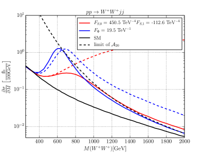
For definiteness, we choose to plot the invariant mass of the vector-boson pair system in the final state, which is the energy scale of the actual VBS process. The initial state is convoluted with the parton structure functions, so the results hold for the LHC (), and we apply standard VBS cuts to enhance the signal. The final-state vector bosons are taken on-shell. We show the distribution for the and final states, where the latter case as the golden channel of VBS is distinguished by the fact that the invariant mass can be reconstructed from the leptonic decays. This is not possible for , but the corresponding same-sign lepton channel is distinguished by a favorable signal-to-background ratio. Note that in the on-shell plots, the vector-boson decay branching ratios have not been included.
In all invariant-mass plots, we display the distribution for the unitarized resonance model (blue curves) together with the pure SM prediction (black). We also plot the unitarity bound for the appropriate partial wave, extrapolated off-shell by the same algorithm, as a dashed curve (black). For illustrative purposes, we also display, in each case, the unitarized extrapolation of the low-energy EFT (red, solid), where we choose the operator coefficients equal to the formal result of integrating out the resonance. Finally, we also display numerical results for the EFT without unitarization (red, dashed) and the resonance with correct width but no further unitarization (blue, dashed).
VI.2.1 Isoscalar-Scalar
The simplest case is a scalar-isoscalar resonance. This is a single isolated resonance, as it could arise, e.g., as the extra scalar particle in a singlet-doublet Higgs model or as a low-energy signal of a strongly interacting Higgs sector that is neutral under the SM gauge group.
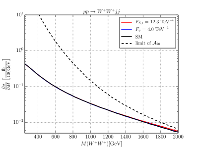
In Fig. 1, upper row, we have selected a moderate mass of and a rather narrow width of , which corresponds to a weak coupling. The isolated resonance is clearly visible in the channel, while the channel is barely affected. For such weak coupling, the operator coefficient in the EFT is small and more than one order of magnitude below the current LHC run-I limit. We can draw the conclusion that in this case the resonance should be detectable for sufficient luminosity, but the EFT approximation is not useful.
Turning to a stronger coupling, we show the corresponding distribution in the channel for and in Fig. 1, lower row.
Here, the EFT parameters are within the range that should become accessible at LHC run II and beyond. The EFT curve (red, solid) appears correctly as the Taylor expansion of the resonance curve (blue) for low energy. However, the energy region where the deviation from the SM becomes sizable, already coincides with the resonance peak region, so the EFT considerably underestimates the event yield. Beyond the resonance, the EFT misses the fact that the distribution falls down again, approaching the SM prediction (black) from above.
The result also demonstrates that the additional unitarization of the scalar resonance beyond the Breit-Wigner approximation with constant width is essential, as is seen by comparing the blue and blue-dashed curves. The naive EFT result without unitarization (red, dashed) grossly overshoots all conceivable models, which should not cross the unitarity limit (black-dashed).
VI.2.2 Isoscalar-Tensor
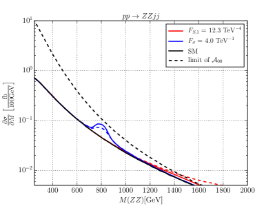
As can be observed from Table 2, a tensor resonance has a stronger impact on the low-energy EFT than a scalar resonance of equal width. In Fig. 2, upper row, we display the distributions for a tensor isoscalar resonance with mass and width .
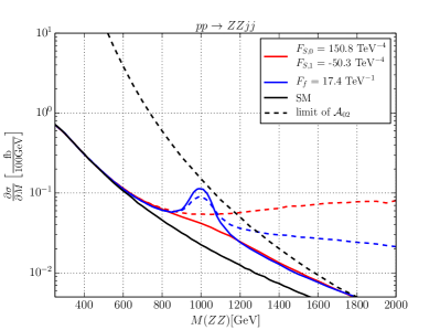
The resonance visibly modifies the distribution already at low energy, such that the EFT analysis, given sufficient sensitivity, should catch the deviation from the SM. Nevertheless, the excess at the peak in the channel is sizable. Beyond the resonance, unitarization is essential in the tensor case. In the final state the tensor enters only as t-channel exchange , so there is no resonance but a broad enhancement. This enhancement is rather well described by the corresponding unitarized EFT 333Tensor resonances resulting in peaks in diboson spectra to explain a recent excess in ATLAS data around 2 TeV can be found e.g. in Fichet:2015yia ..
As in the scalar case, the curves without unitarization do not provide a useful phenomenological description.
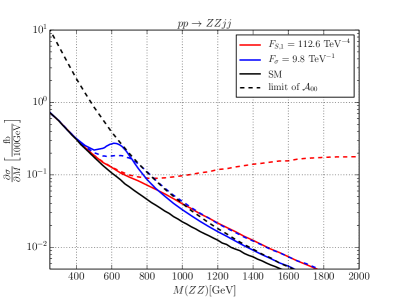
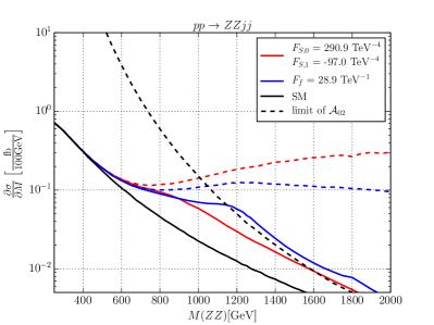
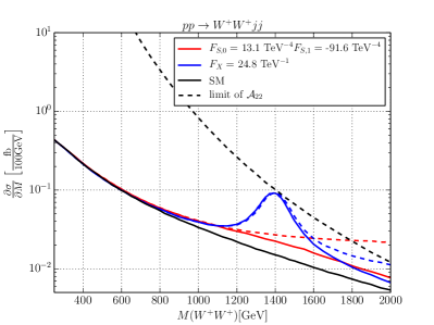
In Fig. 2, lower row, we consider a heavy tensor-isoscalar with strong coupling, and . The resonance peak appears as a broad enhancement, which extends to both low and high energies. The EFT approximation, with sizable coefficients, is rather accurate in this case. The actual resonance curve shows a nontrivial threshold structure which corresponds to the interplay of all partial waves which are excited by s-channel and t-channel exchange contributions. However, we should keep in mind that the prediction for such a strong coupling is uncertain in any case and should not be taken too seriously.
VI.2.3 Isotensor-Scalar
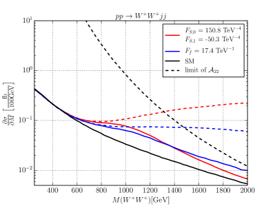
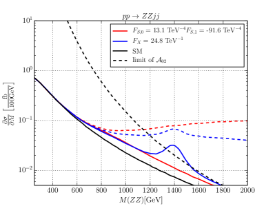
Turning to the isotensor case, we now get a resonance in all final states including . This is illustrated by the plots in Fig. 3 for and .
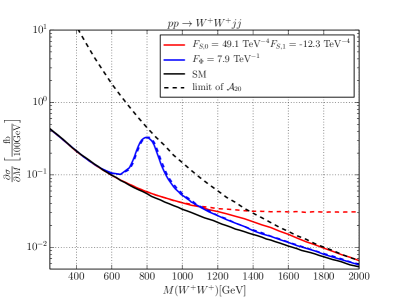
Due to the large number of degrees of freedom (nine states which are degenerate in mass), the peak is rather prominent while the low-energy EFT parameters are again small. We observe that the peak value is slightly below () and above () the appropriate unitarity limit, respectively. This is the effect of -channel exchange which also contributes and can have either sign.
Contrary to the weakly interacting scenario, a non-unitarized low-lying and strongly interacting isotensor-scalar with mass of and width violates the slightly above the resonance as illustrated in Fig. 3. Therefore, a unitarization is needed for this strongly interacting resonance. The low-energy effective field theory approach does only coincide in the unitarized case at high energies, because the eigenamplitudes of the isotensor-scalar as well as the dimension-eight operators are already saturated through the T-matrix formalism.
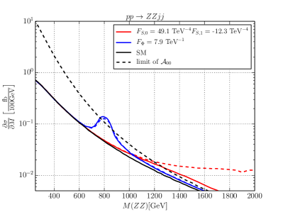
VI.2.4 Isotensor-Tensor
Similarly to the isotensor-scalar, every vector-boson scattering channel receives a resonant contribution from the isotensor-tensor multiplet. The and channel distributions of the isotensor-tensor resonance with mass width are plotted in Fig. 4, upper row. Due to the bound of equation (57), the mass of the isotensor-tensor has to be chosen slightly higher than the mass of the isoscalar-tensor in Fig. 2 when leaving the ratio of width and mass invariant.
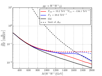
The effective field theory with the dimension-eight operators coincides with the onset of the isotensor-tensor peak. Starting slightly below the resonance, the resonant cross section deviates from the effective field theory description. Analogously to the isotensor-scalar, the very distinctive peak of the isotensor-tensor is not captured by the dimension-eight operators. In the - channel, even the non-unitarized resonance contribution stays within the unitarity bound of . Contrary to the isotensor-scalar, the isotensor-tensor needs unitarization for the final state due to the large tensor contributions in the - and channel. The non-unitarized amplitudes violate the unitarity already below the mass of the resonance. Even the resonance peak is hardly visible. The unitarized resonance curve shows a peak, although it is slightly above the unitarity bound.
In a strongly interacting scenario ( ), the unitarized isotensor-tensor resonance peaks below its actual mass at . This peak originates from the already saturated eigenamplitudes, which then fall due to the parton distribution functions at high energies. Besides the resonance peak, the low-energy effective field theory coincides with the isotensor-tensor for both unitarized and non-unitarized results. This is shown in the lower plot of Fig. 4.
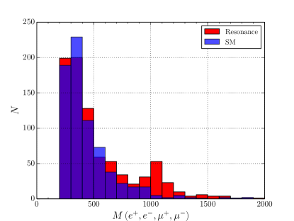
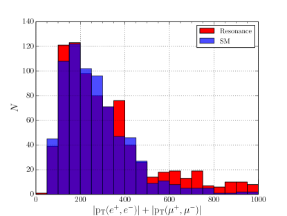
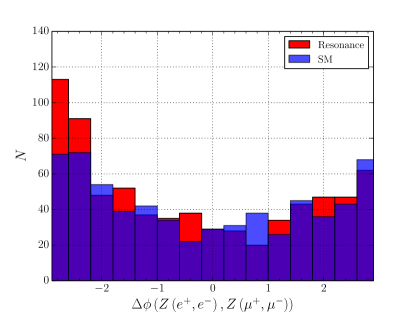
VI.3 Results for Complete Processes
The actual analysis of LHC data will have to exploit cross sections and distributions for the complete final state which consists of the two tagging jets and the decay products of the vector bosons. In this paper, we only investigate the channel with its decay into four leptons, selecting the final state. This process is straightforward to analyze, but suffers from the low leptonic branching ratio, so for our simulation we assume the high-luminosity mode of the LHC with integrated luminosity of . We anticipate that by including also the leptonic final state and hadronic final states, the results can be considerably improved.
The simulation generates event samples for the complete process with all Feynman graphs, so there is no restriction on resonant vector bosons as the origin of the final-state leptons. We apply standard VBS cuts and compare, in Fig. 5, various distributions for the SM (blue), resonance model with a single isoscalar-scalar (red), and the unitarized low-energy EFT (purple).
 |
 |
 |
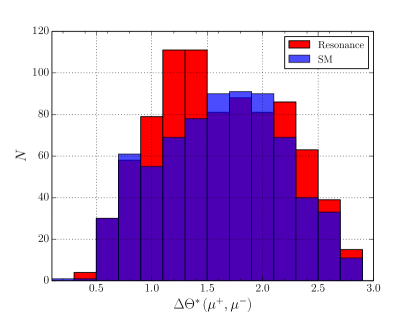 |
The resonance with mass and width appears, as expected, in the invariant mass distribution and, more indirectly, in other plots. Clearly, this parameter set is at the margin of observability in this single channel. The situation obviously improves if we consider resonances with lower mass, larger coupling, in higher representions, and add other analysis channels.
VII Conclusions
The Higgs sector of the SM, after the discovery of a light Higgs, is a new field of study for the experiments at the LHC, and beyond. While the SM yields precise predictions in accordance with the notion of a weakly coupled theory, a thorough analysis of electroweak data should be guided by reference simplified models which differ from the SM. Extending the EFT by higher-dimensional operators is useful for analyzing observables with bounded energy, but open scattering data require enforcing unitarity and extrapolating into a region where perturbation theory in the EFT is insufficient.
Without reference to any particular high-energy model, we have augmented the EFT by resonances with even spin, namely scalar or tensor. Assuming exact gauge invariance and, for simplicity, approximate custodial symmetry both in the EFT and beyond, we can distinguish four distinct resonance multiplets with a single free mass and coupling parameter each. This class of models includes the decoupling limit of multi-Higgs models and certain aspects of massive-graviton models.
The models are set up such that we need only take the interaction with the Higgs sector into account, while couplings to the gauge and fermion sectors occur only via mixing. This is consistent with the symmetry assumptions and with our knowledge about electroweak precision data, although it is clearly not guaranteed. The models allow for arbitrary higher-dimensional operators in the EFT, unrelated to resonance exchange, so we do not lose generality.
All amplitude calculations are meaningless unless we enforce quantum-mechanical unitarity, since naive extrapolations yield event rates in the high-energy region that can exceed the unitarity bounds by orders of magnitude. We have consistently implemented the T-matrix unitarization scheme which works on the complex scattering matrix of the model directly, simplified for the asymptotic range where longitudinal and transveral degrees of freedom decouple.
We have studied the case of a tensor resonance in detail. Since we do not necessarily restrict ourselves to states that are related to gravity, the model differs from the various massive-graviton models and studies that can be found in the literature. To our knowledge, the coupling of a generic tensor resonance to the Higgs sector and the resulting predictions for the LHC have not been considered in detail before. We find that by employing a Stückelberg procedure for the implementation in the Lagrangian, instead of the classic Fierz-Pauli approach, we are able to set up the extended EFT for an isolated tensor resonance manifestly separated from non-resonant effects. Scalar and tensor resonances can be handled in close analogy. It turns out that it is possible to extend an effective theory with an isolated tensor resonance up to a cutoff of order , where is the resonance mass, and is the physical Higgs mass.
We have implemented the models in the Monte-Carlo package WHIZARD and computed exemplary distributions and simulated event samples for the LHC. The numerical results illustrate that resonances in VBS may be detected at the LHC within a certain range of mass and coupling values. For a final verdict, it will be necessary to perform a complete experimental study and analysis, based on exclusive event samples in combination with background and detector description. We also find that the comparison with pure-EFT results can be misleading if resonance and background cannot be clearly separated, as it is typical for the situation at the LHC. We conclude that data should be analyzed on base of resonance models as well as pure-EFT simulations. This holds, in particular, if limits or values are to be combined between distinct final states or with data obtained at a future lepton collider like the ILC Baer:2013cma ; Behnke:2013lya . There has been a first study similar to the one presented here, investigating resonances of spins and isospins zero, one and two in 1 TeV lepton collisions Beyer:2006hx , where issues of unitarization did not play a role.
Acknowledgments
WK and JRR want to thank for the hospitality at the Institute for High Energy Physics (IHEP) and the Center for Future High Energy Physics (CFHEP) of the Chinese Academy of Sciences at Beijing, China, where parts of this work have been completed. MS acknowledges support by JSPS and DAAD and thanks for the hospitality of the KEK theory group during his stay over summer 2015.
Appendix A Notation and conventions
A.1 Fields
| (60) |
To avoid adding terms proportional to the vacuum expectation value, when adding a Higgs pair, we introduce
| (61) |
| (62) | ||||||
The covariant derivative is defined via
| (63) |
and
| (64) |
The equations of motion for the Standard Model yield
| (65a) | ||||
| (65b) | ||||
| (65c) | ||||
| (65d) | ||||
A.2 Tensor Products
The tensor products of Pauli matrices for the isospin quintet , the isospin vector , and the isospin scalar are defined, respectively, as
| (66a) | ||||||
| (66b) | ||||||
| (66c) | ||||||
| (66d) | ||||||
| (66e) | ||||||
| (66f) | ||||||
| (66g) | ||||||
| (66h) | ||||||
| (66i) | ||||||
where the Pauli matrix for the isospin singlet is related to
| (67) |
All nonzero traces of a product of two tensor products are normalized
| (68) |
From the properties of the tensor product
| (69) |
and the trace
| (70) |
we find
| (71) |
This reduces the trace of an isospin singlet
| (72) |
Multiplying the two Pauli matrices related to the isospin singlet leads to
| (73) |
Appendix B Feynman Rules
The Feynman rules which are used to calculate the vector-boson scattering amplitudes are summarized in this appendix. Focusing only on weak vector-boson scattering, the Feynman rules are determined from the Lagrangian, where gluons, photons and fermions are omitted.
B.1 Lagrangian
All Lagrangians are defined within the Higgs matrix realization whose definition can be found in appendix A.1. The Standard Model Lagrangian is given by
| (74) |
Dimension-six and -eight operators affecting only the Higgs/Nambu-Goldstone boson sector are discussed in sections V.4 and are given by
| (75a) | ||||||
| (75b) | ||||||
| (75c) | ||||||
As an extension to model generic new physics, additional resonances are introduced. The scalar resonance and the tensor resonance represent singlets of the chiral symmetry group, whereas has the quantum numbers under . is referred to as isotensor for historical reasons, but it actually includes an isovector and isoscalar besides the isotensor . Also the Fierz-Pauli tensor can be reformulated into a tensor , a vector and a scalar such that canonical propagators can be used for each degree of freedom separately instead of the complicated tensor propagator
| (76a) | ||||
| (76b) | ||||
| (76c) | ||||
| (76d) | ||||
where the projection operator of spin-two states can be written in terms of the spin-one projection operator,
| (77) |
with
| (78) |
B.2 Unitary Gauge
The Feynman rules in unitary gauge of the Lagrangians defined in this paper are listed in this section. Only the relevant vertices for the vector-boson scattering process are shown. In other words, vertices above four fields for effective operators and above three fields for resonances are neglected.
B.2.1 Standard Model
| (79a) | ||||||
| (79b) | ||||||
| (79c) | ||||||
| (79d) | ||||||
| (79e) | ||||||
| (79f) | ||||||
| (79g) | ||||||
| (79h) | ||||||
| (79i) | ||||||
| (79j) | ||||||
B.2.2
| (80a) | ||||||
| (80b) | ||||||
| (80c) | ||||||
| (80d) | ||||||
| (80e) | ||||||
| (80f) | ||||||
B.2.3
| (81a) | ||||||
| (81b) | ||||||
| (81c) | ||||||
| (81d) | ||||||
| (81e) | ||||||
| (81f) | ||||||
B.2.4
| (82a) | ||||||
| (82b) | ||||||
| (82c) | ||||||
B.2.5
| (83a) | ||||||
| (83b) | ||||||
| (83c) | ||||||
| (83d) | ||||||
| (83e) | ||||||
| (83f) | ||||||
| (83g) | ||||||
| (83h) | ||||||
| (83i) | ||||||
B.2.6
| (84a) | ||||||
| (84b) | ||||||
| (84c) | ||||||
B.2.7 in Stückelberg formalism
| (85a) | ||||||
| (85b) | ||||||
| (85c) | ||||||
Because of :
| (86) | ||||||
| (87) | ||||||
| (88) | ||||||
| (89) | ||||||
Because of and :
| (90a) | ||||||
| (90b) | ||||||
| (90c) | ||||||
B.2.8
| (91a) | ||||||
| (91b) | ||||||
| (91c) | ||||||
| (91d) | ||||||
| (91e) | ||||||
| (91f) | ||||||
| (91g) | ||||||
| (91h) | ||||||
| (91i) | ||||||
B.3 Partial wave functions
In this appendix we collect expressions appearing in the partial-wave expansion of amplitudes.
| (92a) | ||||
| (92b) | ||||
| (92c) | ||||
| (92d) | ||||
| (92e) | ||||
| (92f) | ||||
| (92g) | ||||
Appendix C T-matrix Counterterms
In the T-matrix unitarization scheme, the unitarization corrections are expressed as momentum-dependent counterterms for the use as effective Feynman rules in the complete amplitude evaluation. Starting from the spin-isospin eigenamplitudes in the gaugeless limit, section V.2, the straightforward application of the algorithm in Kilian:2014zja yields -dependent amplitude corrections . The insertion as effective Feynman rules proceeds in form of the following expressions:
| (93a) | |||||||
| (93b) | |||||||
| (93c) | |||||||
| (93d) | |||||||
| (93e) | |||||||
| These relations are the generalizations of the corresponding formulae in reference Kilian:2014zja for the case of resonances. Scattering processes involving a Higgs boson have a different off-shell extrapolation. Therefore, the Higgs momentum is included in the Feynman rules for the analogous effective vertices given by | |||||||
| (93f) | |||||||
| (93g) | |||||||
| (93h) | |||||||
| (93i) | |||||||
| (93j) | |||||||
References
- [1] T. Appelquist and J. Carazzone, Phys. Rev. D 11 (1975) 2856.
- [2] K. Hagiwara, S. Ishihara, R. Szalapski and D. Zeppenfeld, Phys. Rev. D 48, 2182 (1993).
- [3] J. F. Gunion and H. E. Haber, Phys. Rev. D 67 (2003) 075019 [hep-ph/0207010].
- [4] H. E. Haber and Y. Nir, Nucl. Phys. B 335 (1990) 363.
- [5] H. E. Haber, arXiv:1401.0152 [hep-ph].
- [6] Y. Nambu, Phys. Rev. Lett. 4, 380 (1960).
- [7] J. Goldstone, Nuovo Cim. 19, 154 (1961).
- [8] J. Goldstone, A. Salam and S. Weinberg, Phys. Rev. 127, 965 (1962).
- [9] C. E. Vayonakis, Lett. Nuovo Cim. 17, 383 (1976).
- [10] M. S. Chanowitz and M. K. Gaillard, Nucl. Phys. B 261, 379 (1985).
- [11] G. J. Gounaris, R. Kogerler and H. Neufeld, Phys. Rev. D 34, 3257 (1986).
- [12] Y. P. Yao and C. P. Yuan, Phys. Rev. D 38, 2237 (1988).
- [13] J. Bagger and C. Schmidt, Phys. Rev. D 41, 264 (1990).
- [14] H. J. He, Y. P. Kuang and X. y. Li, Phys. Rev. Lett. 69, 2619 (1992).
- [15] H. J. He, Y. P. Kuang and X. y. Li, Phys. Lett. B 329, 278 (1994) [hep-ph/9403283].
- [16] H. J. He, Y. P. Kuang and X. y. Li, Phys. Rev. D 49, 4842 (1994).
- [17] H. J. He and W. B. Kilgore, Phys. Rev. D 55, 1515 (1997) [hep-ph/9609326].
- [18] G. Aad et al. [ATLAS Collaboration], Phys. Rev. Lett. 113, no. 14, 141803 (2014) [arXiv:1405.6241 [hep-ex]].
- [19] The ATLAS collaboration [ATLAS Collaboration], ATLAS-CONF-2014-013.
- [20] CMS Collaboration [CMS Collaboration], CMS-PAS-FSQ-13-008.
- [21] S. Weinberg, Phys. Rev. Lett. 17, 616 (1966).
- [22] M. S. Chanowitz, M. Golden and H. Georgi, Phys. Rev. D 36, 1490 (1987).
- [23] B. W. Lee, C. Quigg and H. B. Thacker, Phys. Rev. Lett. 38, 883 (1977); Phys. Rev. D 16, 1519 (1977).
- [24] D. Espriu and F. Mescia, Phys. Rev. D 90, no. 1, 015035 (2014) [arXiv:1403.7386 [hep-ph]].
- [25] R. L. Delgado, A. Dobado and F. J. Llanes-Estrada, Phys. Rev. D 91, no. 7, 075017 (2015) [arXiv:1502.04841 [hep-ph]].
- [26] T. Appelquist and C. W. Bernard, Phys. Rev. D 22, 200 (1980).
- [27] A. C. Longhitano, Phys. Rev. D 22, 1166 (1980).
- [28] D. A. Dicus, J. F. Gunion and R. Vega, Phys. Lett. B 258, 475 (1991).
- [29] V. D. Barger, K. m. Cheung, T. Han and R. J. N. Phillips, Phys. Rev. D 42, 3052 (1990).
- [30] M. S. Berger and M. S. Chanowitz, Phys. Lett. B 263, 509 (1991).
- [31] S. N. Gupta, J. M. Johnson and W. W. Repko, Phys. Rev. D 48, 2083 (1993) [hep-ph/9307239].
- [32] T. Appelquist and G. H. Wu, Phys. Rev. D 48, 3235 (1993) [hep-ph/9304240].
- [33] M. S. Chanowitz, Phys. Lett. B 373, 141 (1996) [hep-ph/9512358].
- [34] J. Bagger, V. D. Barger, K. m. Cheung, J. F. Gunion, T. Han, G. A. Ladinsky, R. Rosenfeld and C.-P. Yuan, Phys. Rev. D 52, 3878 (1995) [hep-ph/9504426].
- [35] J. M. Butterworth, B. E. Cox and J. R. Forshaw, Phys. Rev. D 65, 096014 (2002) [hep-ph/0201098].
- [36] O. J. P. Eboli, M. C. Gonzalez-Garcia and S. M. Lietti, Phys. Rev. D 69, 095005 (2004) [hep-ph/0310141].
- [37] O. J. P. Eboli, M. C. Gonzalez-Garcia and J. K. Mizukoshi, Phys. Rev. D 74, 073005 (2006) [hep-ph/0606118].
- [38] J. Distler, B. Grinstein, R. A. Porto and I. Z. Rothstein, Phys. Rev. Lett. 98, 041601 (2007) [hep-ph/0604255].
- [39] T. Han, D. Krohn, L. T. Wang and W. Zhu, JHEP 1003, 082 (2010) [arXiv:0911.3656 [hep-ph]].
- [40] A. Freitas and J. S. Gainer, Phys. Rev. D 88, no. 1, 017302 (2013) [arXiv:1212.3598].
- [41] D. Espriu and B. Yencho, Phys. Rev. D 87, no. 5, 055017 (2013) [arXiv:1212.4158 [hep-ph]].
- [42] K. Doroba, J. Kalinowski, J. Kuczmarski, S. Pokorski, J. Rosiek, M. Szleper and S. Tkaczyk, Phys. Rev. D 86, 036011 (2012) [arXiv:1201.2768 [hep-ph]].
- [43] J. Chang, K. Cheung, C. T. Lu and T. C. Yuan, Phys. Rev. D 87, 093005 (2013) [arXiv:1303.6335 [hep-ph]].
- [44] R. L. Delgado, A. Dobado and F. J. Llanes-Estrada, arXiv:1412.3277 [hep-ph].
- [45] M. Fabbrichesi, M. Pinamonti, A. Tonero and A. Urbano, arXiv:1509.06378 [hep-ph].
- [46] M. Szleper, arXiv:1412.8367 [hep-ph].
- [47] A. Alboteanu, W. Kilian and J. Reuter, JHEP 0811, 010 (2008) [arXiv:0806.4145 [hep-ph]].
- [48] W. Kilian, T. Ohl, J. Reuter and M. Sekulla, Phys. Rev. D 91 (2015) 096007 [arXiv:1408.6207 [hep-ph]].
- [49] I. Antoniadis, Phys. Lett. B 246 (1990) 377.
- [50] N. Arkani-Hamed, S. Dimopoulos and G. R. Dvali, Phys. Lett. B 429 (1998) 263 [hep-ph/9803315].
- [51] I. Antoniadis, N. Arkani-Hamed, S. Dimopoulos and G. R. Dvali, Phys. Lett. B 436 (1998) 257 [hep-ph/9804398]. [52]
- [52] T. Han, J. D. Lykken and R. J. Zhang, Phys. Rev. D 59, 105006 (1999) [hep-ph/9811350].
- [53] N. Bouatta, G. Compere and A. Sagnotti, hep-th/0409068.
- [54] L. P. S. Singh and C. R. Hagen, Phys. Rev. D 9 (1974) 898.
- [55] I. L. Buchbinder and V. A. Krykhtin, Nucl. Phys. B 727 (2005) 537 [hep-th/0505092].
- [56] S. -Z. Huang, P. -F. Zhang, T. -N. Ruan, Y. -C. Zhu and Z. -P. Zheng, Eur. Phys. J. C 42 (2005) 375.
- [57] M. Sekulla Ph.D. thesis, University of Siegen, 2015
- [58] R. D. Ball and R. S. Thorne, Annals Phys. 241 (1995) 368 [hep-th/9404156].
- [59] C. Fronsdal, Il Nuovo Cimento (1955-1965) 9 (1958) 2.
- [60] S. Weinberg, Phys. Rev. 133 (1964) B1318.
- [61] M. Fierz and W. Pauli, Proc. Roy. Soc. Lond. A 173 (1939) 211.
- [62] N. Arkani-Hamed, H. Georgi and M. D. Schwartz, Annals Phys. 305 (2003) 96 [hep-th/0210184].
- [63] N. Arkani-Hamed and M. D. Schwartz, Phys. Rev. D 69 (2004) 104001 [hep-th/0302110].
- [64] M. D. Schwartz, Phys. Rev. D 68 (2003) 024029 [hep-th/0303114].
- [65] C. de Rham, G. Gabadadze and A. J. Tolley, Phys. Lett. B 711 (2012) 190 [arXiv:1107.3820 [hep-th]].
- [66] S. F. Hassan, A. Schmidt-May and M. von Strauss, Phys. Lett. B 715 (2012) 335 [arXiv:1203.5283 [hep-th]].
- [67] J. Noller, J. H. C. Scargill and P. G. Ferreira, JCAP 1402 (2014) 007 [arXiv:1311.7009 [hep-th]].
- [68] K. Hinterbichler, Rev. Mod. Phys. 84 (2012) 671 [arXiv:1105.3735 [hep-th]].
- [69] E. C. G. Stueckelberg, Helv. Phys. Acta 11, 225 (1938).
- [70] E. C. G. Stueckelberg, Helv. Phys. Acta 15 (1942) 23.
- [71] H. Ruegg and M. Ruiz-Altaba, Int. J. Mod. Phys. A 19 (2004) 3265 [hep-th/0304245].
- [72] J. Bonifacio, P. G. Ferreira and K. Hinterbichler, Phys. Rev. D 91 (2015) 125008 [arXiv:1501.03159 [hep-th]].
- [73] C. P. Burgess and D. London, hep-ph/9203215.
- [74] S. Weinberg, Phys. Rev. 166, 1568 (1968); W. Kilian, Springer Tracts Mod. Phys. 198, 1 (2003).
- [75] D. B. Kaplan and H. Georgi, Phys. Lett. B 136, 183 (1984).
- [76] For reviews of Little Higgs models cf.: M. Schmaltz and D. Tucker-Smith, Little Higgs review, Ann. Rev. Nucl. Part. Sci. 55, 229 (2005) [hep-ph/0502182]; M. Perelstein, Little Higgs models and their phenomenology, Prog. Part. Nucl. Phys. 58, 247 (2007) [hep-ph/0512128]; EWPT, Fine-tuning have been studied here: W. Kilian and J. Reuter, Phys. Rev. D 70, 015004 (2004) [hep-ph/0311095]. J. Reuter and M. Tonini, JHEP 1302, 077 (2013) [arXiv:1212.5930 [hep-ph]]. J. Reuter, M. Tonini and M. de Vries, arXiv:1307.5010 [hep-ph]; JHEP 1402, 053 (2014) [arXiv:1310.2918 [hep-ph]].
- [77] W. Kilian, T. Ohl and J. Reuter, WHIZARD: Simulating Multi-Particle Processes at LHC and ILC, Eur. Phys. J. C 71, 1742 (2011) [arXiv:0708.4233 [hep-ph]].
- [78] M. Moretti, T. Ohl and J. Reuter, O’Mega: An Optimizing matrix element generator, In *2nd ECFA/DESY Study 1998-2001* 1981-2009 [hep-ph/0102195].
- [79] W. Kilian, T. Ohl, J. Reuter and C. Speckner, JHEP 1210, 022 (2012) [arXiv:1206.3700 [hep-ph]].
- [80] W. Kilian, J. Reuter, S. Schmidt and D. Wiesler, JHEP 1204, 013 (2012) [arXiv:1112.1039 [hep-ph]].
- [81] N. D. Christensen, C. Duhr, B. Fuks, J. Reuter and C. Speckner, Eur. Phys. J. C 72, 1990 (2012) [arXiv:1010.3251 [hep-ph]].
- [82] B. Chokoufe Nejad, W. Kilian, J. Reuter and C. Weiss, PoS EPS -HEP2015, 317 (2015) [arXiv:1510.02739 [hep-ph]]; C. Weiss, B. Chokoufe Nejad, W. Kilian and J. Reuter, PoS EPS -HEP2015, 466 (2015) [arXiv:1510.02666 [hep-ph]]; N. Greiner, A. Guffanti, T. Reiter and J. Reuter, Phys. Rev. Lett. 107, 102002 (2011) [arXiv:1105.3624 [hep-ph]]; T. Binoth, N. Greiner, A. Guffanti, J. Reuter, J.-P. Guillet and T. Reiter, Phys. Lett. B 685, 293 (2010) [arXiv:0910.4379 [hep-ph]]; W. Kilian, J. Reuter and T. Robens, Eur. Phys. J. C 48, 389 (2006) [hep-ph/0607127].
- [83] S. Fichet and G. von Gersdorff, arXiv:1508.04814 [hep-ph].
- [84] H. Baer et al., arXiv:1306.6352 [hep-ph].
- [85] T. Behnke et al., arXiv:1306.6329 [physics.ins-det].
- [86] M. Beyer, W. Kilian, P. Krstonosic, K. Mönig, J. Reuter, E. Schmidt and H. Schröder, Eur. Phys. J. C 48, 353 (2006) [hep-ph/0604048].