Vertical Equilibrium, Energetics, and Star Formation Rates in Magnetized Galactic Disks Regulated by Momentum Feedback from Supernovae

Abstract

Recent hydrodynamic (HD) simulations have shown that galactic disks evolve to reach well-defined statistical equilibrium states. The star formation rate (SFR) self-regulates until energy injection by star formation feedback balances dissipation and cooling in the interstellar medium (ISM), and provides vertical pressure support to balance gravity. In this paper, we extend our previous models to allow for a range of initial magnetic field strengths and configurations, utilizing three-dimensional, magnetohydrodynamic (MHD) simulations. We show that a quasi-steady equilibrium state is established as rapidly for MHD as for HD models unless the initial magnetic field is very strong or very weak, which requires more time to reach saturation. Remarkably, models with initial magnetic energy varying by two orders of magnitude approach the same asymptotic state. In the fully saturated state of the fiducial model, the integrated energy proportions $E_{\rm turb}:E_{\rm th}:\delta E_{\rm mag}:\overline{E}_{\rm mag}$ are $0.35:0.39:0.15:0.11$, while the proportions of midplane support $P_{\rm turb}:P_{\rm th}:\delta\Pi_{\rm mag}:\overline{\Pi}_{\rm mag}$ are $0.49:0.18:0.18:0.15$. Vertical profiles of total effective pressure satisfy vertical dynamical equilibrium with the total gas weight at all heights. We measure the “feedback yields” $\eta_{c}\equiv P_{c}/\Sigma_{\rm SFR}$ (in suitable units) for each pressure component, finding that $\eta_{\rm turb}\sim 4$ and $\eta_{\rm th}\sim 1$ are the same for MHD as in previous HD simulations, and $\delta\eta_{\rm mag}\sim 1$. These yields can be used to predict the equilibrium SFR for a local region in a galaxy based on its observed gas and stellar surface densities and velocity dispersions. As the ISM weight (or dynamical equilibrium pressure) is fixed, an increase in $\eta$ from turbulent magnetic fields reduces the predicted $\Sigma_{\rm SFR}$ by $\sim 25\%$ relative to the HD case.

1 Introduction

The diffuse atomic interstellar medium (ISM), the mass reservoir in galaxies from which molecular clouds and stars are born, is highly turbulent (e.g., Elmegreen & Scalo, 2004) and strongly magnetized (e.g., Beck, 2001). The roles of turbulence and magnetic fields in the context of star formation have been emphasized many times (see Shu et al., 1987; Mac Low & Klessen, 2004; McKee & Ostriker, 2007, for reviews). Additionally, the importance of turbulence and magnetic fields on large scales is clear from comparison of each component’s pressure to the vertical weight of the ISM disk (e.g. Boulares & Cox, 1990; Ferrière, 2001). In the Solar neighborhood, representing fairly typical conditions among star forming galactic disks, turbulent and magnetic pressures are roughly comparable to each other (e.g., Heiles & Troland, 2005), and about three times larger than the thermal pressure in diffuse gas (e.g., Jenkins & Tripp, 2011). Therefore, turbulence and magnetic fields provide most of the vertical support to the gas layer, and are essential to include in models of the vertical structure in galactic disks. Moreover, the magnetic field has a significant random component (see Haverkorn, 2015, for recent review), which presumably is related to observed turbulent velocities. This implies an intriguing additional dimension to models in which the star formation rate (SFR) is connected to the vertical dynamical equilibrium of the ISM disk via turbulence driven by star formation feedback (Ostriker et al., 2010; Ostriker & Shetty, 2011; Kim et al., 2011).

Another important characteristic of the diffuse atomic ISM is its multiphase nature, which emerges naturally as a consequence of thermal instability with a realistic treatment of cooling and heating (Field, 1965). The temperature and density of the cold and warm medium differ by about two orders of magnitude (Field et al., 1969; Wolfire et al., 1995, 2003). The inhomogeneous, multiphase structure of the diffuse atomic ISM is observed to be ubiquitous (e.g., Heiles & Troland, 2003; Dickey et al., 2009; Roy et al., 2013; Murray et al., 2015). In addition to the warm and cold phases, the hot phase that is created by supernovae (SNe) is an essential ISM component (Cox & Smith, 1974; McKee & Ostriker, 1977; Ferrière, 2001). This phase contains very little mass, but is of great dynamical importance because the expansion of high-pressure SN remnants and superbubbles is the main driver of turbulence in the surrounding denser phases of the ISM (and also drives galactic winds) (de Avillez & Breitschwerdt, 2004; Joung & Mac Low, 2006; Joung et al., 2009; Hill et al., 2012; Creasey et al., 2013; Li et al., 2015).

Owing to the huge difference between cooling and dynamical times and correspondingly large range of spatial scales, directly modeling the multiphase ISM is numerically quite challenging. However, the combination of increasing computational resources, with robust algorithms for evolving gas dynamics and thermodynamics simultaneously, have enabled development of highly sophisticated ISM models in the last decade. Direct numerical simulations of vertically stratified galactic disks with SN driven turbulence and stiff source terms to follow heating and cooling include those of de Avillez & Breitschwerdt (2004, 2005); Joung & Mac Low (2006); Joung et al. (2009); Hill et al. (2012); Gent et al. (2013a); Kim et al. (2011, 2013); Hennebelle & Iffrig (2014); Walch et al. (2014). Among those, only Kim et al. (2013, hereafter Paper I) and Hennebelle & Iffrig (2014) have a time-dependent SFR and SN rate self-consistently set by the self-gravitating localized collapse of gas.

The time-dependent response of the SFR to large-scale ISM dynamics and thermodynamics is key to self-consistent regulation of turbulent and thermal pressures, since both the turbulent driving rate (from SNe) and thermal heating rate (from far-UV-emitting massive stars) are proportional to the SFR. If heating rates and turbulent driving rates drop due to a low SFR, the increased mass of cold, dense gas subsequently leads to a rebound in the SFR. The opposite is also true, with an excessively high SFR checked by the ensuing reduction in the mass of gas eligible to collapse. Within less than an orbital time, the SFR self-regulates such that the ISM achieves a statistical equilibrium state. In this state, there are balances between (1) vertical gravity and the combined pressure forces, (2) turbulent driving and dissipation, and (3) cooling and heating (see Ostriker et al. 2010; Ostriker & Shetty 2011; Kim et al. 2011 for analytic theory, and Kim et al. 2011, Paper I; Shetty & Ostriker 2012, Paper I for numerical confirmations). Paper I successfully reproduces important aspects of the diffuse atomic ISM, demonstrating self-regulated SFR and vertical equilibrium following the analytic theory for a range of galactic conditions including those of the Solar neighborhood as well as regions with higher and lower total ISM surface density. In addition, the warm/cold ratios and properties of 21 cm emission/absorption for H I (including column density and spin temperature distributions) are in agreement with observations (Kim et al., 2014).

Despite of the success of hydrodynamic (HD) models in Paper I, the dynamical role of magnetic fields cannot be ignored. For example, Hennebelle & Iffrig (2014) have run magnetized ISM disk models with self-gravity and SN feedback, showing a factor of two decrement in the SFR compared to the HD case. However, a systematic exploration of the effect of magnetic fields is still lacking. In this paper, a set of three-dimensional, magnetohydrodynamic (MHD) simulations is carried out, to test the effects of different initial magnetic field strengths and configuration.

The remainder of the paper is organized as follows. In Section 2, we begin by reviewing the analytic theory and previous simulation results to identify and explain the properties and parameters we will measure here. Section 3 summarizes our numerical methods and model parameters. Our basis is the fiducial Solar neighborhood model from Paper I with gas surface density of 10$\;{\rm M}_{\odot}\;{\rm pc^{-2}}$, but here we slightly alter the initial and boundary conditions to minimize early vertical oscillations that were exaggerated in Paper I. Section 4 contains our main new results. Time evolution of disk diagnostics in Section 4.1 shows that a quasi-steady state is achieved. In Section 4.2, we analyze temporally and horizontally averaged vertical profiles to confirm vertical dynamical equilibrium. Finally, Section 4.3 presents the measurements of “feedback yields,” exploring the mutual relationship between measured SFR surface density and the various midplane pressure supports. We compare the numerical results with analytic expectations including magnetic terms. In Section 5, we summarize and discuss the model disk properties at saturation in comparison to observations and previous simulations, especially focusing on the level of mean and turbulent magnetic fields.

2 The Equilibrium Theory

Before describing the results of our new simulations, it is informative to summarize the analytic theory for mutual equilibrium of the ISM and star formation in disk systems, as developed in our previous work (Ostriker et al., 2010; Ostriker & Shetty, 2011; Kim et al., 2011). This includes a list of the parameters to be measured for detailed investigation. The equilibrium theory assumes a quasi-steady state that satisfies force balance between vertical gravity and pressure support, and energy balance between gains from star formation feedback and losses in the dissipative ISM. We shall test the validity of these assumptions and quantify the relative contributions to the vertical support from turbulent, thermal, and magnetic terms. We shall also measure the efficiency of feedback (feedback yield) for each support term.

Using the temporally- and horizontally- averaged momentum equation, it is straightforward to show that vertical dynamical equilibrium requires a balance between the total momentum flux difference between surfaces at $z=0$ and $z_{\rm max}$, and the weight of the gas: $\Delta P_{\rm tot}=\mathcal{W}$. In magnetized, turbulent galactic disks, the vertical momentum flux consists of thermal ($P_{\rm th}\equiv\rho v_{\rm th}^{2}$), turbulent ($P_{\rm turb}\equiv\rho v_{z}^{2}$), and magnetic ($\Pi_{\rm mag}\equiv|\mathbf{B}|^{2}/8\pi-B_{z}^{2}/4\pi$) terms (e.g., Boulares & Cox, 1990; Piontek & Ostriker, 2007; Ostriker & Shetty, 2011). Note that the magnetic term includes both pressure and tension, and can be rewritten as $\Pi_{\rm mag}=\rho(v_{A}^{2}/2-v_{A,z}^{2})$, where $v_{A}\equiv\left(|\mathbf{B}|^{2}/4\pi\rho\right)^{1/2}$ is the Alfvén velocity from the total magentic field and $v_{A,z}=|B_{z}|/(4\pi\rho)^{1/2}$ is from its $z$ component. We hereafter refer to $\Pi_{\rm mag}$ as the magnetic “support” to distinguish from the usual magnetic “pressure” ($P_{\rm mag}\equiv|\mathbf{B}|^{2}/8\pi$), while the thermal and turbulent “supports” are equivalent to the thermal and turbulent “pressures,” respectively. If we choose $z_{\rm max}$ where the gas density is sufficiently small, $P_{\rm th}(z_{\rm max})$, $P_{\rm turb}(z_{\rm max})\rightarrow 0$ by definition, but $\Pi_{\rm mag}(z_{\rm max})$ can in general be nonzero and significant. We thus have

$$\Delta P_{\rm tot}={P_{\rm th}}_{,0}+{P_{\rm turb}}_{,0}+\Delta\Pi_{\rm mag}\equiv\rho_{0}\sigma_{z}^{2}(1+\mathcal{R}),$$ (1)

where $\sigma_{z}^{2}\equiv v_{\rm th}^{2}+v_{z}^{2}$ is the sum of thermal and turbulent velocity dispersions, and

$$\mathcal{R}\equiv\frac{\Delta\Pi_{\rm mag}}{\rho_{0}\sigma_{z}^{2}}$$ (2)

is the relative contribution to the vertical support from magnetic to kinetic (thermal plus turbulent) terms. If $\mathbf{B}(z_{\rm max})\rightarrow 0$, $\Delta\Pi_{\rm mag}\rightarrow(|\mathbf{B}_{0}|^{2}/2-B_{z,0}^{2})/4\pi$. Here and hereafter, we use the subscript ‘0’ to indicate quantities evaluated at the midplane ($z=0$),

The weight of the gas under self- and external gravity is respectively defined by

$$\mathcal{W}_{\rm sg}=\int_{0}^{z_{\rm max}}\rho\frac{d\Phi_{\rm sg}}{dz}dz=\frac{\pi G\Sigma^{2}}{2}$$ (3)

and

$$\mathcal{W}_{\rm ext}=\int_{0}^{z_{\rm max}}\rho g_{\rm ext}(z)dz\equiv\zeta_{d}g_{\rm ext}(H)\Sigma$$ (4)

Here, $\Sigma\equiv\int_{-\infty}^{\infty}\rho dz$ is the gaseous surface density, $H\equiv\Sigma/(2\rho_{0})$ is the gaseous disk’s effective scale height, and $\zeta_{d}\equiv(1/2)\int_{0}^{z_{\rm max}}\rho|g_{\rm ext}(z)/g_{\rm ext}(H)|dz/\int_{0}^{z_{\rm max}}\rho dz$ is a dimensionless parameter that characterizes the vertical distribution of gas and the shape of external gravity profile. For example, with linear external gravity profile ($g_{\rm ext}\propto z$), density following exponential, Gaussian, and sech² distributions gives $\zeta_{d}=1/2$, $1/\pi$, and $(\ln 2)/2$, respectively.

We now specialize to the case of a galactic disk with a midplane density of stars + dark matter equal to $\rho_{\rm sd}$, for which the external gravity near the midplane is $g_{\mathrm{ext}}=4\pi G\rho_{\rm sd}z$. Vertical dynamical equilibrium can be expressed as

$$\rho_{0}\sigma_{z}^{2}(1+\mathcal{R})=\mathcal{W}_{\rm sg}(1+\chi),$$ (5)

where

$$\chi\equiv\frac{\mathcal{W}_{\rm ext}}{\mathcal{W}_{\rm sg}}=\frac{4\zeta_{d}\rho_{\rm sd}}{\rho_{0}}$$ (6)

is the ratio of external to self gravity. By substituting from Equation (3) for $\mathcal{W}_{\rm sg}$ and from Equation (6) for $\chi$ in Equation (5), we can solve to obtain

$$H=H_{\rm sg}\frac{1+\mathcal{R}}{1+\chi}=H_{\rm ext}\left({\frac{1+\mathcal{R}}{1+1/\chi}}\right)^{1/2},$$ (7)

where $H_{\rm sg}\equiv\sigma_{z}^{2}/\pi G\Sigma$ and $H_{\rm ext}\equiv\sigma_{z}/(8\pi G\zeta_{d}\rho_{\rm sd})^{1/2}$ are the scale heights for self- and external- gravity dominated cases, respectively. By defining

$$C\equiv\frac{H_{\rm sg}^{2}}{H_{\rm ext}^{2}}=\frac{8\zeta_{d}\rho_{\rm sd}\sigma_{z}^{2}}{\pi G\Sigma^{2}},$$ (8)

Equation (7) can also be solved for $\chi$ to obtain

$$\chi=\frac{2C(1+\mathcal{R})}{1+\sqrt{1+4C(1+\mathcal{R})}}.$$ (9)

If we neglect dark matter and consider a stellar disk with surface density $\Sigma_{*}$ and vertical stellar velocity dispersion $\sigma_{*}$ such that $\rho_{\rm sd}\rightarrow\pi G\Sigma_{*}^{2}/(2\sigma_{*}^{2})$, we have

$$C(1+\mathcal{R})=4\zeta_{d}\left({\frac{\sigma_{\mathrm{eff}}\Sigma_{*}}{\sigma_{*}\Sigma}}\right)^{2}.$$ (10)

Here,

$$\sigma_{\mathrm{eff}}\equiv\left(v_{\rm th}^{2}+v_{z}^{2}+\frac{v_{A}^{2}}{2}-v_{A,z}^{2}\right)^{1/2}=\sigma_{z}(1+\mathcal{R})^{1/2}$$ (11)

is the effective vertical velocity dispersion including magnetic terms for gaseous support, and we have assumed that $\mathbf{B}(z_{\rm max})\rightarrow 0$.

We shall show from results of our simulations in Section 4.1 that $\sigma_{\mathrm{eff}}\sim 5-6\;{\rm km}\;{\rm s}^{-1}$ and $\zeta_{d}\sim 0.4-0.5$ are quite insensitive to the initial magnetization (see Tables 1 and 2). In Paper I, we also found relatively little variation in $\sigma_{z}$, even with a factor 10 variation in $\Sigma$ and two orders of magnitude variation of $\rho_{\rm sd}/\Sigma^{2}$, the input parameter that controls the ratio of external- to self-gravity. In this paper, we fix $\Sigma$ and $\rho_{\rm sd}$ to isolate the effect of magnetic fields. Further investigations would therefore be needed to investigate constancy or variation of $\sigma_{\mathrm{eff}}$ and $\zeta_{d}$ with $\Sigma$ and $\rho_{\rm sd}$, which we defer to future work.

In simulations, $\Sigma$ and $\rho_{\rm sd}$ (as well as a seed magnetic field) are input parameters, and $\sigma_{z}$, $\mathcal{R}$, and $\zeta_{d}$ are measured outputs. From the right-hand side of Equation (5) combined with Equations (9) and (8), the predicted dynamical equilibrium midplane pressure can be obtained. In observed (relatively face-on) galactic disks, the gas and stellar surface densities $\Sigma$ and $\Sigma_{*}$ together with $\sigma_{z}$ and $\sigma_{*}$ may be considered basic observables (although the stellar scale height $H_{*}=\sigma_{*}^{2}/(\pi G\Sigma_{*})$ instead may be estimated in other ways if $\sigma_{*}$ is not directly measured; e.g. Leroy et al., 2008). The magnetic term $v_{A}^{2}/2-v_{A,z}^{2}$ in $\sigma_{\mathrm{eff}}^{2}$ is more difficult to measure directly. We shall show, however, that if the model disk is fully saturated, $\mathcal{R}=(v_{A}^{2}/2-v_{A,z}^{2})/\sigma_{z}^{2}$ appears to be insensitive to the initial magnetic geometry or strength. This implies that the predicted equilibrium midplane pressure support may similarly be obtained from observables using Equations (5), (9), (10), (11) if estimates of $\mathcal{R}$ and $\zeta_{d}$ from simulations are adopted.

To test the validity of vertical dynamical equilibrium, for our simulations we will compare full vertical profiles of the total (turbulent, thermal, and magnetic) support with the vertical profiles of the weight of the gas. These profiles are based on horizontal and temporal averages of the simulation outputs at all values of $z$, including the midplane. In equilibrium, the weight and total support profiles must match each other.

Due to the highly dissipative nature of the ISM, continuous energy injection is necessary to maintain thermal as well as turbulent kinetic and magnetic components of the vertical support at a given level. Massive young stars inject prodigious energy, providing the feedback that is key to self-regulation of the SFR. When the system is out of equilibrium, with not enough massive young stars, lack of energy injection leads the entire ISM to become dynamically and thermally cold. A cold disk is highly susceptible to gravitational collapse; it forms new stars that supply the “missing” feedback and restore equilibrium. In the opposite case, with too many massive stars, the ISM becomes dynamically and thermally hot, quenching further star formation by suppressing gravitational instability. Simulations of local model disks show that the SFR converges to the quasi-steady value predicted by theory, in which the vertical support produced by feedback matches the requirements set by vertical dynamical equilibrium. The ISM state and SFR predicted by the feedback-regulated theory are expected to hold in real galaxies provided all equilibria can be established in less than the disk’s secular evolution timescale.

In Paper I (see also Kim et al., 2011; Shetty & Ostriker, 2012), we showed that the balance between energy gains and losses is established within one vertical crossing time, the turbulence dissipation timescale. We then quantified the efficiency of energy conversion to each support component for a given SFR by measuring the “feedback yield.”

Using a suitable normalization, we define yield parameters $\eta_{c}$ as

$$\eta_{c}\equiv\frac{P_{c,3}}{\Sigma_{\rm SFR,-3}}$$ (12)

where $P_{c,3}=P_{c,0}/10^{3}k_{\rm B}\;{\rm cm}^{-3}\,{\rm K}$ and $\Sigma_{\rm SFR,-3}=\Sigma_{\rm SFR}/10^{-3}\;{\rm M}_{\odot}\;{\rm kpc}^{-2}\;{\rm yr}^{-1}$. The subscript ‘$c$’ denotes “turb,” “th,” or “mag” for the respective component of vertical support ($P_{\rm turb}$, $P_{\rm th}$, or $\Pi_{\rm mag}$). For magnetic pressure, the support is further divided into turbulent and mean components, $\delta\Pi_{\rm mag}$ and $\overline{\Pi}_{\rm mag}$, respectively (see Section 4.1 for definitions). Ostriker et al. (2010) and Ostriker & Shetty (2011) respectively showed that $\eta_{\rm th}$ and $\eta_{\rm turb}$ are expected to be nearly independent of $\Sigma_{\rm SFR}$. In Paper I (see also Kim et al., 2011), which omitted magnetic fields but covered a wide range of disk conditions such that $0.1<\Sigma_{\rm SFR,-3}<10$, we obtained $\eta_{\rm turb}=4.3\Sigma_{\rm SFR,-3}^{-0.11}$ and $\eta_{\rm th}=1.3\Sigma_{\rm SFR,-3}^{-0.14}$. The values (and weak $\Sigma_{\rm SFR}$ dependence) of these numerically calibrated yield parameters are in very good agreement with analytic expectations.

The MHD simulations of this paper allow us to study the evolution and saturated-state properties of magnetic fields in star-forming, turbulent, differentially-rotating galactic disks with vertical stratification. ISM turbulence driven by star formation feedback can generate and deform magnetic fields. The small scale turbulent dynamo, combined with buoyancy and sheared rotation, creates turbulent magnetic fields and modifies mean magnetic fields, both of which can provide vertical support to the ISM. We shall consider three different initial magnetic field strengths (as well as two initial vertical profiles), and directly measure the saturated-state magnetic field strengths and feedback yields, while also testing how magnetization affects the thermal and turbulent feedback yield components.

3 Methods and Models

In this paper, we extend our previous three dimensional HD simulations from Paper I to include magnetic fields. We solve ideal MHD equations in a local, shearing box with self- and external gravity, thermal conduction, and optically thin cooling. To solve the MHD equations, we utilize Athena (Stone et al., 2008) with the van Leer integrator (Stone & Gardiner, 2009), HLLD solver, and second-order spatial reconstruction. We also consider feedback from massive young stars using time-varying heating rate and momentum feedback from SNe. The probability of massive star formation is calculated based on a predicted local SFR ($\dot{M}_{*}$) in cells with density exceeding a threshold, assuming an efficiency per free-fall time $\epsilon_{\rm ff}=1\%$ (e.g., Krumholz & Tan, 2007), and adopting a total mass in new stars per massive star of $m_{*}=100\;{\rm M}_{\odot}$. When a massive star forms (i.e., when a uniform random number in (0,1) is less than the probability $\dot{M}_{*}/m_{*}\Delta t$), we immediately inject total radial momentum $p_{*}=3\times 10^{5}\;{\rm M}_{\odot}\;{\rm km}\;{\rm s}^{-1}$ in a surrounding $10\;{\rm pc}$ sphere. The global SFR surface density is then calculated by

$$\Sigma_{\rm SFR}=\frac{\mathcal{N}_{*}m_{*}}{L_{x}L_{y}t_{\rm bin}},$$ (13)

where $\mathcal{N}_{*}$ denotes the total number of massive stars in the time interval $(t-t_{\rm bin},t)$, and $t_{\rm bin}=10\;{\rm Myr}$ is UV-weighted lifetime of OB stars (e.g., Parravano et al., 2003). The heating rate is proportional to the mean FUV intensity, which is assumed to be linearly proportional to the SFR surface density, $\Gamma\propto J_{\rm FUV}\propto\Sigma_{\rm SFR}$. See Paper I for more details and other source terms.

The models in this paper are magnetically-modified versions of the fiducial simulation QA10 from Paper I, with conditions similar to the Solar neighborhood. Our simulation domain is a local Cartesian grid far from the galactic center, with center rotating at angular velocity of $\Omega=28\;{\rm km}\;{\rm s}^{-1}\;{\rm kpc}^{-1}$ (the corresponding orbital time is $t_{\rm orb}=2\pi/\Omega=219\;{\rm Myr}$) and shear parameter $q\equiv-d\ln\Omega/d\ln R=1$ for a flat rotation curve. In the $\hat{z}$ direction, we adopt outflow boundary conditions to allow magnetic flux loss at the vertical boundaries; this is in contrast to Paper I, where we adopted periodic vertical boundary conditions (except for the gravitational potential) to prevent any mass loss. In order to minimize mass loss at the vertical boundaries, we double the vertical domain size to $L_{z}=1024\;{\rm pc}$ compared to Paper I. Shearing-periodic boundary conditions are employed in the horizontal directions, with $L_{x}=L_{y}=512\;{\rm pc}$ the same as in Paper I. The spatial resolution is set to $2\;{\rm pc}$ as in Paper I. We adopt a linear external gravity profile $\mathbf{g}_{\rm ext}=-4\pi G\rho_{\rm sd}z\hat{\mathbf{z}}$, where $\rho_{\rm sd}$ is the midplane volume density of stellar disk plus dark matter.

In order to explore the independent effect of the magnetic fields, we fix the background gravity and gas surface density parameters to $\rho_{\rm sd}=0.05\;{\rm M}_{\odot}\;{\rm pc^{-3}}$ and $\Sigma=10\;{\rm M}_{\odot}\;{\rm pc^{-2}}$ for all models. Initial profiles of the gas density are set by an exponential function as $\rho=\rho_{0}\exp(-|z|/H)$, with midplane density $\rho_{0}=\Sigma/2H$ and scale height set using $\sigma_{z}=4\;{\rm km}\;{\rm s}^{-1}$ in Equations (7) and (8), also using $\zeta_{d}=1/2$ and $\mathcal{R}$ as described below. The initial thermal pressure has the same profile as the density with midplane thermal pressure of $P_{\rm th,0}/k_{\rm B}=3000\;{\rm cm}^{-3}\,{\rm K}$. We vary the plasma beta at the midplane $\beta_{0}\equiv P_{\rm th,0}/P_{\rm mag,0}=8\pi P_{\rm th,0}/B_{0}^{2}$ with two different vertical field distributions; uniform plasma beta with $\mathbf{B}=B_{0}\exp(-|z|/2H)\hat{\mathbf{y}}$ (Models MA), and uniform magnetic fields with $\mathbf{B}=B_{0}\hat{\mathbf{y}}$ (Models MB). The suffixes of magnetized models denote the values of $\beta_{0}=1$, 10, and 100. The initial magnetic energy is then largest for Model MB1 and smallest for Model MA100. For comparison, we also present the results from an unmagnetized counterpart (Model HL) as well as the previous Model QA10 from Paper I (here, renamed HS). These hydrodynamic models differ in the size of the vertical domain (“S”=small, $L_{z}=512$ pc; “L”=large, $L_{z}=1024$ pc).

For our initial conditions, we have $\zeta_{d}=1/2$ and $C=2.37$ for all models. With vertically stratified magnetic fields (Models MA; $\mathcal{R}=1/\beta_{0}$), $\chi=1.12$, 1.13, 1.19, and 1.73 for $\beta_{0}=\infty$, 100, 10, and 1, respectively, while $\chi=1.12$ for all MB models ($\mathcal{R}=0$). The scale height is $H=77[(1+\mathcal{R})(1+1/\chi)]^{1/2}\;{\rm pc}$ and $n_{\rm H,0}=\rho_{0}/1.4\;m_{\rm H}=1.9[(1+\mathcal{R})(1+1/\chi)]^{-1/2}\;{\rm cm}^{-3}$. The midplane magnetic field strength is

$$B_{0}=3.2\beta_{0}^{-1/2}\left({\frac{P_{\rm th,0}/k_{\rm B}}{3000\;{\rm cm}^{-3}\,{\rm K}}}\right)^{1/2}\mu G.$$ (14)

In contrast to Paper I, we drive turbulence for $t_{\rm orb}$ in order to provide turbulent support at early stages before SN feedback generates sufficient turbulence. We utilize divergence-free turbulent velocity fields following a Gaussian random distribution with a power spectrum of the form $|\delta\mathbf{v}_{k}^{2}|\propto k^{6}\exp(-8k/k_{\rm pk})$ where the peak driving is at $k_{\rm pk}L_{x}/2\pi=4$ and $1\geq kL_{x}/2\pi\geq 128$. A new turbulent velocity perturbation field is generated every $10\;{\rm Myr}$, with total energy injection rate of $\dot{E}_{\rm turb}=500L_{\odot}$ to the turbulence. This perturbation corresponds to the saturation level of one-dimensional velocity dispersion $\sim 4\;{\rm km}\;{\rm s}^{-1}$. Turbulence is driven at full strength up to $t_{\rm orb}/2$, and then slowly turned off from $t_{\rm orb}/2$ to $t_{\rm orb}$. The spatially uniform photoelectric heating rate is set to constant for the first $t_{\rm orb}/2$ ($\Gamma=0.8\Gamma_{0}$, where $\Gamma_{0}=2\times 10^{-26}\;{\rm erg}\;{\rm s}^{-1}$ from Koyama & Inutsuka 2002). From $t_{\rm orb}/2$ to $t_{\rm orb}$ this imposed heating is slowly turned off and replaced by the self-consistent heating rate that is proportional to the SFR surface density ($\Gamma=0.4\Gamma_{0}\Sigma_{\rm SFR,-3}$).

By initially driving turbulence, and allowing smooth changes from early to saturated stages in the thermal and turbulent supports, the current models minimize abrupt early collapse that was seen in the models of Paper I that were initialized without turbulence (as reproduced in model HS here). There, the initial vertical collapse also triggered a strong burst of star formation, leading to exaggerated vertical oscillations. However, we shall show that these and other differences in numerical treatment (including initial turbulence driving, vertical boundary conditions, and domain size) make little or no differences in the physical quantities (see Section 4.1) and averaged vertical distributions (see Section 4.2). Since some magnetized models saturate slowly, we run magnetized models longer to achieve a quasi-steady state for the turbulent magnetic fields. For the purpose of computing time-averaged quantities, the saturated stages are considered from $t_{1}=3t_{\rm orb}$ to $t_{2}=4t_{\rm orb}$ for magnetized models and from $t_{1}=1.5t_{\rm orb}$ to $t_{2}=2t_{\rm orb}$ for unmagnetized models. Note that 4 orbits is still not long enough for complete saturation of the mean magnetic field in the cases of initially strongest and weakest magnetization.

4 Simulation Results

4.1 Time Evolution and Saturated State

In this section, we shall show that model disks achieve a quasi-steady state, using evolution of diagnostics that describe the average disk properties at a given time. Volume and mass-weighted means for quantities $q_{ijk}(t)$ are respectively calculated by

$$\left\langle{q}\right\rangle_{V}(t)\equiv\frac{\sum q\Delta V}{L_{x}L_{y}L_{z}},\quad\left\langle{q}\right\rangle_{M}(t)\equiv\frac{\sum\rho q\Delta V}{\sum\rho\Delta V},$$ (15)

where the summation is over all grid zones (indices $ijk$), and the volume element is $\Delta V=(2\;{\rm pc})^{3}$. We also calculate the horizontally-averaged vertical profile as

$$\overline{q}(z;t)\equiv\frac{\sum_{i,j}q\Delta x\Delta y}{L_{x}L_{y}},$$ (16)

where the summation is only over horizontal planes (indices $ij$) at each vertical coordinate $z$ (index $k$).

We use a horizontal average to obtain the mean magnetic field, $\overline{\mathbf{B}}(z)$. The turbulent magnetic field is then defined by $\delta\mathbf{B}=\mathbf{B}-\overline{\mathbf{B}}$. Note that in our simulations the mean field is dominated by $\hat{\mathbf{y}}$-component with small $\hat{\mathbf{x}}$-component and negligible $\hat{\mathbf{z}}$-component. The turbulent magnetic pressure is given by $\delta P_{\mathrm{mag}}\equiv|\delta\mathbf{B}|^{2}/8\pi$ and the mean magnetic pressure is given by $\bar{P}_{\mathrm{mag}}\equiv|\bar{\mathbf{B}}|^{2}/8\pi$.

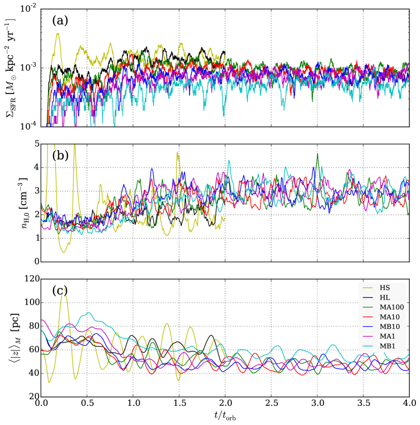
Figure 1: Time evolution of (a) SFR surface density $\Sigma_{\rm SFR}$, (b) midplane number density $n_{\rm H,0}$, and (c) mass-weighted mean thickness $\left\langle{|z|}\right\rangle_{M}$. Physical model parameters differ only in the initial magnetic energy, increasing from zero in HS and HL to a maximum in MB1 (see Section 3).

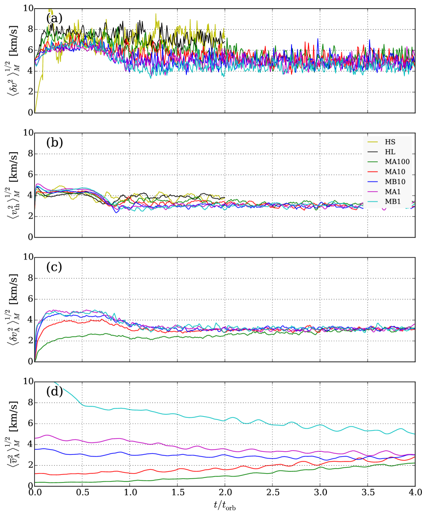
Figure 2: Time evolution of mass-weighted RMS (a) turbulent kinetic, (b) thermal, (c) turbulent Alfvén and (d) mean Alfvén velocity.

Table 1: Mean Disk Properties at Saturation

Model	$\Sigma_{\rm SFR}$	$n_{\rm H,0}$	$\langle{|z|}\rangle_{M}$	$H$	$\zeta_{d}$	$\chi$	$\alpha_{\rm ss,R}$	$\alpha_{\rm ss,M}$
HS	$1.59\pm 0.38$	$1.96\pm 0.56$	$61.5\pm 10.4$	$73.8\pm 21.1$	$0.42\pm 0.14$	$1.23\pm 0.54$	$0.22\pm 0.07$	$\cdots$
HL	$1.46\pm 0.28$	$2.15\pm 0.41$	$60.6\pm 6.3$	$67.3\pm 12.9$	$0.45\pm 0.10$	$1.21\pm 0.35$	$0.25\pm 0.10$	$\cdots$
MA100	$0.91\pm 0.16$	$2.87\pm 0.45$	$47.1\pm 3.1$	$50.3\pm 7.9$	$0.47\pm 0.08$	$0.94\pm 0.22$	$0.22\pm 0.13$	$0.23\pm 0.07$
MA10	$0.81\pm 0.16$	$2.87\pm 0.35$	$47.4\pm 4.2$	$50.4\pm 6.2$	$0.47\pm 0.07$	$0.95\pm 0.18$	$0.22\pm 0.09$	$0.27\pm 0.07$
MB10	$0.74\pm 0.15$	$2.85\pm 0.31$	$47.6\pm 3.6$	$50.7\pm 5.5$	$0.47\pm 0.06$	$0.95\pm 0.16$	$0.21\pm 0.09$	$0.32\pm 0.08$
MA1	$0.75\pm 0.16$	$3.00\pm 0.37$	$48.2\pm 4.2$	$48.2\pm 6.0$	$0.50\pm 0.08$	$0.96\pm 0.19$	$0.23\pm 0.10$	$0.22\pm 0.10$
MB1	$0.56\pm 0.14$	$2.97\pm 0.43$	$55.1\pm 4.3$	$48.7\pm 7.0$	$0.57\pm 0.09$	$1.10\pm 0.24$	$0.17\pm 0.09$	$0.27\pm 0.10$

Note. — The mean and standard deviation are taken over $t/t_{\rm orb}=1.5-2$ for HD models and $t/t_{\rm orb}=3-4$ for MHD models. See Sections 2 and 4.1 for definition of each quantity. $\Sigma_{\rm SFR}$ is in units of $10^{-3}\;{\rm M}_{\odot}\;{\rm kpc}^{-2}\;{\rm yr}^{-1}$, $n_{\rm H,0}$ is in units of $\rm cm^{-3}$, $\left\langle{|z|}\right\rangle_{M}$ and $H$ are in units of pc.

Table 2: Saturated State Velocities

Model	$\langle\delta v^{2}\rangle_{M}^{1/2}$	$\langle v_{\rm th}^{2}\rangle_{M}^{1/2}$	$\langle\delta v_{A}^{2}\rangle_{M}^{1/2}$	$\langle\overline{v}_{A}^{2}\rangle_{M}^{1/2}$	$\sigma_{\rm z}$	$\sigma_{\mathrm{eff}}$
HS	$7.31\pm 0.65$	$3.89\pm 0.20$	$\cdots$	$\cdots$	$5.96\pm 0.36$	$5.96\pm 0.36$
HL	$6.95\pm 0.53$	$3.89\pm 0.16$	$\cdots$	$\cdots$	$5.67\pm 0.27$	$5.67\pm 0.27$
MA100	$5.22\pm 0.55$	$3.16\pm 0.13$	$3.07\pm 0.13$	$1.93\pm 0.17$	$4.36\pm 0.28$	$4.78\pm 0.27$
MA10	$5.10\pm 0.55$	$3.07\pm 0.16$	$3.18\pm 0.10$	$2.47\pm 0.17$	$4.27\pm 0.29$	$4.83\pm 0.25$
MB10	$4.89\pm 0.55$	$3.01\pm 0.15$	$3.19\pm 0.12$	$2.74\pm 0.13$	$4.17\pm 0.30$	$4.81\pm 0.27$
MA1	$4.94\pm 0.52$	$3.05\pm 0.17$	$3.15\pm 0.14$	$3.16\pm 0.15$	$4.21\pm 0.28$	$4.97\pm 0.24$
MB1	$4.46\pm 0.45$	$3.09\pm 0.17$	$3.19\pm 0.16$	$5.39\pm 0.22$	$4.11\pm 0.27$	$5.78\pm 0.22$

Note. — The mean and standard deviation are taken over $t/t_{\rm orb}=1.5-2$ for HD models and $t/t_{\rm orb}=3-4$ for MHD models. See Sections 2 and 4.1 for definition of each quantity. All velocities are in units of km/s. Figure 3 for detailed statistical information about energies related to each velocity component.

Figures 1 and 2 plot time evolution of selected diagnostics that describe overall disk properties and energetics. In Figure 1, we plot (a) SFR surface density $\Sigma_{\rm SFR}$, (b) midplane number density $n_{\rm H,0}=\overline{\rho}_{0}/(1.4\;m_{\rm H})$ and (c) mass-weighted mean height $\left\langle{|z|}\right\rangle_{M}$. Figure 2 plots mass weighted means of (a) three-dimensional turbulent velocity $\langle\delta v^{2}\rangle_{M}^{1/2}$, (b) sound speed $\langle v_{\rm th}^{2}\rangle_{M}^{1/2}$, and (c) turbulent $\langle\delta{v}_{A}^{2}\rangle_{M}^{1/2}$ and (d) mean $\langle\overline{v}_{A}^{2}\rangle_{M}^{1/2}$ Alfvén velocities. Here, we subtract the azimuthal velocity arising from the background shear (not the horizontal average) for turbulent velocity, $\delta\mathbf{v}\equiv\mathbf{v}+q\Omega x\hat{\mathbf{y}}$. The mean and standard deviations of values from Figure 1 are listed in Table 1. Time averages are taken over the “saturated state” time interval of $(t_{1},t_{2})$. We also list in Table 1 the mean and standard deviation of $H=\Sigma/2\rho_{0}$, $\zeta_{d}=\left\langle{|z|}\right\rangle_{M}/2H$, and $\chi=4\zeta_{d}\rho_{\rm sd}/\rho_{0}$. In Table 2, we report the mean and standard deviations of the velocities shown in Figure 2, as well as $\sigma_{z}=[\langle v_{\rm th}^{2}\rangle_{M}+\langle v_{z}^{2}\rangle_{M}]^{1/2}$, and $\sigma_{\mathrm{eff}}=[\sigma_{z}^{2}+\langle v_{A}^{2}\rangle_{M}/2-\langle v_{A,z}^{2}\rangle_{M}]^{1/2}$.

Comparing Models HS (yellow) and HL (black), Figure 1 shows distinct differences at early stages ($t<t_{\rm orb}$), but no systematic differences in mean values of physical quantities at later stages. In Model HS, initial vertical collapse at $t\sim 20\;{\rm Myr}$ triggers an abrupt increase of $n_{\rm H,0}$ and hence $\Sigma_{\rm SFR}$, which then produces feedback that causes a strong reduction in $n_{\rm H,0}$ and $\Sigma_{\rm SFR}$, leading to further bounces. These exaggerated vertical oscillations are a direct consequence of the lack of turbulence in the initial conditions and early evolution, before feedback has developed. In contrast to Model HS, Model HL (and all magnetized models) shows no strong oscillation at early stages, although more limited vertical oscillation emerges and persists at later times. The early driven turbulence and constant heating in Model HL (and magnetized models) prevent strong, global vertical oscillations, keeping the midplane density and the thickness of the disk more or less constant. Without initial vertical collapse, there is no bursting star formation; rather, the SFR in Model HL remains moderate. After one orbit time, when the turbulence driving and heating are fully self-consistent with feedback from the star formation, all diagnostics in the unmagnetized models quickly saturate. The convergence of Models HS and HL to the same saturated state, despite their completely different early evolution, confirms the robustness of our previous work.

The magnetized models also achieve a quasi-steady state, but not so rapidly as the unmagnetized models. Even after saturation of thermal and turbulent velocities (both $\delta v$ and $\delta v_{A}$) as well as the midplane density and scale height at $\sim 2t_{\rm orb}$, clear secular evolution continues for the mean Alfvén velocity (or mean magnetic fields; see Figure 2(d)). The models with initially strongest magnetic fields (MA1 and MB1) slowly lose energy from the mean magnetic field as buoyant magnetic fields escape through the vertical boundaries. Conversely, the mean magnetic energy of models with initially weakest magnetic fields (MA100 and MA10) slowly grows. We note, however, that since our horizontal dimension is only 512 pc and assumed to be periodic, magnetic energy loss might be somewhat overestimated in our simulations compared to the case in which azimuthal fields are anchored at larger scales. In principle, if numerical reconnection in our models is faster than realistic small-scale reconnection (which is uncertain) should be, we might also overestimate the growth of mean magnetic fields in weak-field models. Modulo these potential numerical effects, the interesting tendency seen in Figure 2(d) is that $\langle\overline{v}_{A}^{2}\rangle_{M}^{1/2}$ converges toward similar values for cases with widely varying initial magnetic fields.

The magnetized models show distinguishably different final saturated states compared to the unmagnetized models. The SFR surface density and turbulent and thermal velocity dispersions are lower in the magnetized models, while variations among the set of magnetized models is small. This is completely consistent with expectations from the equilibrium theory, in which (1) the sum of all pressures must offset a given ISM weight, so the addition of magnetic pressure reduces the need for turbulent and thermal pressure, and (2) an increase in “feedback yields” due to magnetic fields implies that a lower star formation rate is needed for equilibrium. We examine this issue in detail in Section 4.3.

Similarities and differences among models are clearest in the energetics. In Figure 2, we clearly see the saturation of turbulent and thermal velocity dispersions for all models immediately after $t_{\rm orb}$. The turbulent Alfvén velocity also converges rapidly except in Model MA100, which converges after $3t_{\rm orb}$. Model MB10 achieves a quasi-steady state earliest among the magnetized models since it has initial magnetic energy comparable to that of the final state. We thus consider Model MB10 as the fiducial run. All other magnetized models converge toward the same saturated state as Model MB10. As seen in Figure 2 and Table 2, the saturated-state values of $\langle\delta{v}^{2}\rangle_{M}^{1/2}$, $\langle v_{\rm th}^{2}\rangle_{M}^{1/2}$, and $\langle\delta{v}_{A}^{2}\rangle_{M}^{1/2}$, are essentially indistinguishable for all magnetized models, whereas $\langle\overline{v}_{A}^{2}\rangle_{M}^{1/2}$ values show some variations as they have not yet reached asymptotic values.

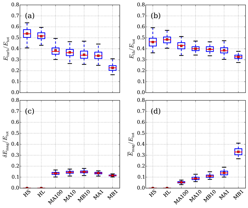
Figure 3: Box and whisker plot of the energy ratios (a) turbulent (kinetic) $E_{\rm turb}/E_{\rm tot}$, (b) thermal $E_{\rm th}/E_{\rm tot}$, (c) turbulent magnetic $\delta E_{\rm mag}/E_{\rm tot}$, and (d) mean magnetic $\overline{E}_{\rm mag}/E_{\rm tot}$, averaged over $(t_{1},t_{2})$. The bottom and top of the rectangular box denote the first ($Q_{1}$) and third ($Q_{3}$) quartiles, respectively, while the red line within the box is the median (second quartile; $Q_{2}$) of the data. The lower/upper whisker reaches to $1.5\times(Q_{3}-Q_{1})$ or the minimum/maximum of the data, whichever is larger/smaller.

In Figure 3, we summarize the saturated-state energy ratios with “box and whisker” plots omitting outliers, and with the mean values (red squares). From left to right in each panel, the initial degree of magnetization increases. Panels show the fraction of total energy in each component: turbulent kinetic, thermal, turbulent magnetic, and mean magnetic. The turbulent kinetic energy is defined by $E_{\rm turb}\equiv\sum\Delta V\rho|\delta\mathbf{v}|^{2}/2$, and the thermal energy is $E_{\rm th}=\sum\Delta VP_{\rm th}/(\gamma-1)$, where $\gamma=5/3$ in our simulations. The mean and turbulent magnetic energies are given by $\overline{E}_{\rm mag}\equiv\sum\Delta V|\overline{\mathbf{B}}|^{2}/8\pi$ and $\delta E_{\rm mag}\equiv\sum\Delta V|\delta\mathbf{B}|^{2}/8\pi$. Since $\overline{\delta\mathbf{B}}=0$ by definition, $E_{\rm mag}=\overline{E}_{\rm mag}+\delta E_{\rm mag}$. Note that these energies are integrated over the whole volume, which compared to the midplane (see Section 4.2 and Table 3) increases the relative proportion of thermal to turbulent energy.

For the unmagnetized models, the turbulent kinetic and thermal energies are nearly in equipartition. For Model MB10, which is the most saturated magnetized model, the total energy is portioned into kinetic (35%), thermal (39%), turbulent magnetic (15%), and mean magnetic (11%) terms. Thus, kinetic, thermal, and magnetic components are each close to 1/3 of the total energy. The ratio between turbulent kinetic and turbulent magnetic energies is about $E_{\rm turb}:\delta E_{\rm mag}=7:3$, similar to what has been found for saturation of small scale dynamo simulations at large Reynolds number (e.g. Haugen et al., 2004, see Section 5 for details). Although the mean magnetic energy is not yet fully saturated (see Figure 2(d)) for all models, there is a clear trend of convergence toward the saturated state of Model MB10. Figure 2 and Table 2 show that component energies in the magnetized models are nearly the same except the mean magnetic term, which still reflects initial mean field strengths.

It is of interest to characterize the angular momentum transport by both turbulence and magnetic fields in our models. We measure the $R$-$\phi$ component of Reynolds and Maxwell stresses as a function of $z$, $R_{xy}\equiv\overline{\rho v_{x}\delta v_{y}}$ and $M_{xy}\equiv\overline{B_{x}B_{y}/4\pi}$, respectively. Since the stresses are non-negligible only within one gas scale height, it is most informative to calculate the mass-weighted mean values of the stresses normalized by the mean midplane thermal pressure, the “$\alpha_{\mathrm{ss}}$-parameters” of Shakura & Sunyaev (1973): $\alpha_{\mathrm{ss,R}}=\left\langle{R_{xy}}\right\rangle_{M}/\overline{P}_{\rm th,0}$ and $\alpha_{\mathrm{ss,M}}=\left\langle{M_{xy}}\right\rangle_{M}/\overline{P}_{\rm th,0}$ (see Table 3 for $\overline{P}_{\rm th,0}$). As listed in Table 1, the $\alpha_{\mathrm{ss}}$-parameters are comparable to each other and $\sim 0.2-0.3$. Although the ratio between Reynolds and Maxwell stresses is completely different compared to the the case of turbulence driven by magnetorotational instability (where the Maxwell stress dominates), the total stress $\sim 0.4-0.5$ is similar (e.g., Hawley et al., 1995; Kim et al., 2003; Piontek & Ostriker, 2005). Note that gravitational stress in our simulations is generally lower, with $\alpha_{\mathrm{ss}}\sim 0.05$. This is also true for other simulations in which turbulence is driven by gravitational instability combined with sheared rotation, which give $\alpha_{\mathrm{ss}}$ less than $0.1$ (e.g., Shi & Chiang, 2014). The total stress gives $\alpha_{\mathrm{ss}}\sim 0.4-0.5$, implying that the gas accretion time $t_{\rm acc}\sim R^{2}\Omega/(\alpha_{\rm ss}v_{\rm th}^{2})=390\;{\rm Gyr}$ for $v_{\rm th}=3\;{\rm km}\;{\rm s}^{-1}$ using $R=8$ kpc.

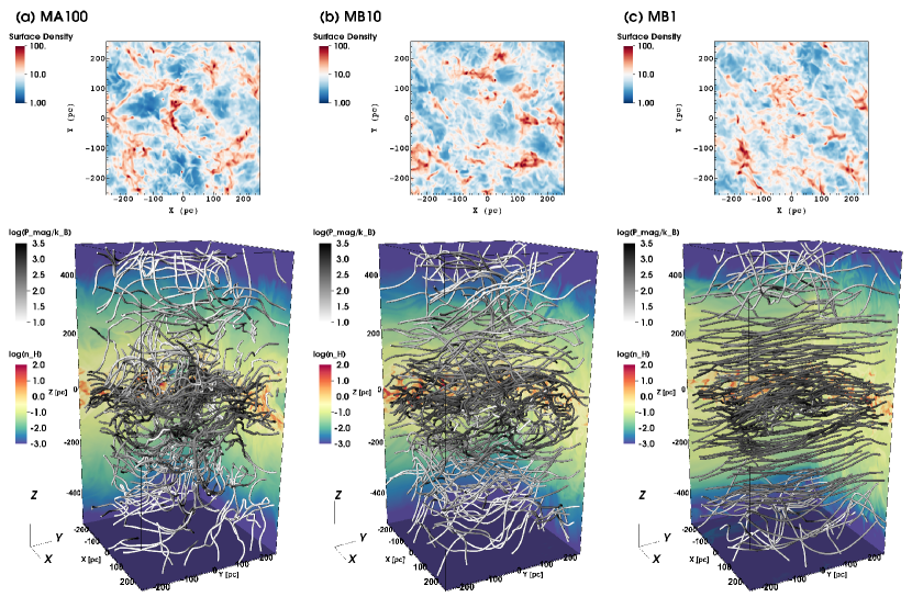
Figure 4: Gas and magnetic structure in Models (a) MA100, (b) MB10, and (c) MB1 at $t/t_{\rm orb}=3$. Top: Surface density in units of $\;{\rm M}_{\odot}\;{\rm pc^{-2}}$. Bottom: 3D visualization of magnetic field lines, with vertical slices of hydrogen number density shown in color scale on box boundaries. Model MB1 shows field lines preferentially along $\hat{\mathbf{y}}$ within $|z|<300\;{\rm pc}$ since its mean magnetic fields are still dominant. From right to left, randomness of the magnetic field structure increases as the mean field strength decreases, since the turbulent field strengths are all similar at this time. Differences in the magnetic field produce no clear signature in surface density maps, however, with similar cloudy structure in all cases.

To illustrate the overall saturated-state disk structure, in Figure 4 we display surface density (top) and magnetic field lines (bottom) for Models (a) MA100, (b) MB10, and (c) MB1 at $t/t_{\rm orb}=3$. As shown in Figures 2 and 3, the strength of the mean magnetic field increases from MA100 to MB10 to MB1 (from left to right in Figure 4). Averaged over the saturation period ($t/t_{\rm orb}=3-4$), the mean and turbulent magnetic field values at the midplane are $\overline{\mathbf{B}}=(-0.26,1.2,0)\;\mu{\rm G}$ and $\delta\mathbf{B}_{\rm rms}=(1.3,1.6,1.1)\;\mu{\rm G}$ for Model MA100, $\overline{\mathbf{B}}=(-0.30,1.7,0)\;\mu{\rm G}$ and $\delta\mathbf{B}_{\rm rms}=(1.4,1.7,1.2)\;\mu{\rm G}$ for Model MB10, and $\overline{\mathbf{B}}=(-0.15,2.5,0)\;\mu{\rm G}$ and $\delta\mathbf{B}_{\rm rms}=(1.4,1.8,1.2)\;\mu{\rm G}$ for Model MB1. For all models, the azimuthal ($\hat{y}$) component is the largest of $\overline{\mathbf{B}}$. However, this component exceeds the turbulent components only for model MB1; for model MB10 it is comparable to the largest turbulent component, and for model MB100 it is smaller than the largest turbulent component. As a result, field lines are more complex and random in Model MA100 ($\delta E_{\rm mag}>\overline{E}_{\rm mag}$) and more aligned in a preferential direction (along $\hat{\mathbf{y}}$) in Model MB1 ($\delta E_{\rm mag}<\overline{E}_{\rm mag}$). The dominance of the mean magnetic fields at all heights in Model MB1 is also evident.

Despite of the strong distinctions in the structure of field lines, the surface density maps look quite similar for all models. In particular, there is no visually prominent evidence of alignment of dense filaments either perpendicular or parallel to the mean magnetic field direction. However, traces of the shear are evident in overall pattern of striations (consistent with trailing wavelets), particularly for Model MB1. More quantitative analysis of the morphology of filaments and magnetic field lines may be obtained using maps of synthetic 21 cm emission, dust emission, and polarization (e.g., Soler et al., 2013; Planck Collaboration et al., 2015). We defer this interesting study to future work.

4.2 Vertical Dynamical Equilibrium

In this subsection, we investigate the vertical dynamical equilibrium of model disks using horizontally and temporally averaged profiles of $P_{\rm turb}$, $P_{\rm th}$, $\delta\Pi_{\rm mag}$, and $\overline{\Pi}_{\rm mag}$, in comparison to profiles of the ISM weight $\mathcal{W}$. We also compare midplane values.

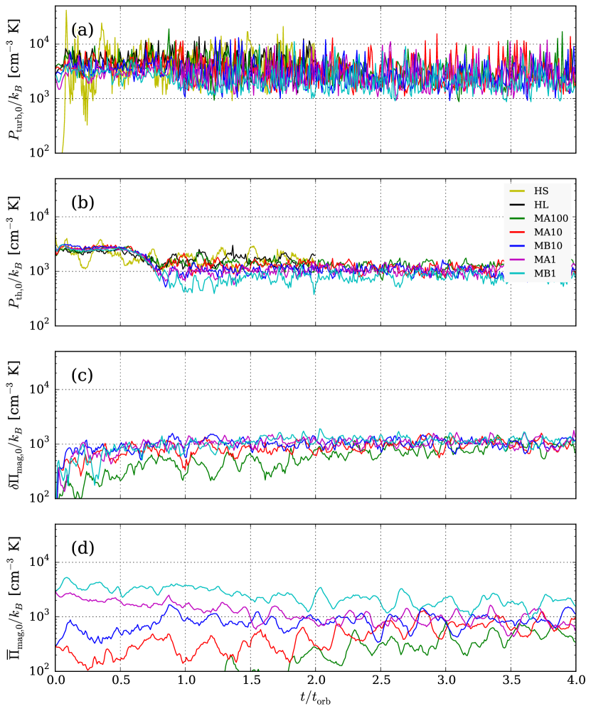
Figure 5: Time evolution of horizontally-averaged components of support at the midplane: (a) turbulent kinetic $P_{\rm turb}$, (b) thermal $P_{\rm th}$, (c) turbulent magnetic $\delta\Pi_{\rm mag}$, and (d) mean magnetic $\overline{\Pi}_{\rm mag}$.

Table 3: Vertical Support and Feedback Yield at Saturation

Model	$P_{\rm turb}$	$P_{\rm th}$	$\delta\Pi_{\rm mag}$	$\overline{\Pi}_{\rm mag}$	$\eta_{\rm turb}$	$\eta_{\rm th}$	$\delta\eta_{\rm mag}$
HS	$5.24\pm 3.05$	$1.78\pm 0.40$	$\cdots$	$\cdots$	$3.30\pm 2.08$	$1.12\pm 0.37$	$\cdots$
HL	$5.15\pm 2.61$	$1.61\pm 0.29$	$\cdots$	$\cdots$	$3.53\pm 1.91$	$1.10\pm 0.29$	$\cdots$
MA100	$3.40\pm 2.42$	$1.24\pm 0.18$	$0.94\pm 0.21$	$0.46\pm 0.15$	$3.72\pm 2.73$	$1.35\pm 0.31$	$1.03\pm 0.29$
MA10	$3.38\pm 2.66$	$1.14\pm 0.20$	$1.04\pm 0.18$	$0.73\pm 0.18$	$4.17\pm 3.38$	$1.41\pm 0.36$	$1.29\pm 0.33$
MB10	$2.85\pm 1.46$	$1.04\pm 0.18$	$1.03\pm 0.17$	$0.87\pm 0.23$	$3.83\pm 2.12$	$1.40\pm 0.38$	$1.38\pm 0.37$
MA1	$3.02\pm 2.11$	$1.05\pm 0.16$	$1.10\pm 0.22$	$0.91\pm 0.29$	$4.00\pm 2.92$	$1.39\pm 0.37$	$1.46\pm 0.43$
MB1	$2.18\pm 1.12$	$0.83\pm 0.16$	$1.16\pm 0.18$	$1.83\pm 0.45$	$3.92\pm 2.23$	$1.49\pm 0.47$	$2.08\pm 0.61$

Note. — The mean and standard deviation are taken over $t/t_{\rm orb}=1.5-2$ for HD models and $t/t_{\rm orb}=3-4$ for MHD models. The vertical support terms at the midplane ($P_{\rm turb}$, $P_{\rm th}$, $\delta\Pi_{\rm mag}$, and $\overline{\Pi}_{\rm mag}$) are given in units of $10^{3}k_{\rm B}\;{\rm cm}^{-3}\,{\rm K}$. See Equation (12) for $\eta$ definition and Figure 9 for detailed statistical information about feedback yields.

Figure 5 plots time evolution of horizontally-averaged midplane support terms: (a) $P_{\rm turb}$, (b) $P_{\rm th}$, (c) $\delta\Pi_{\rm mag}$, and (d) $\overline{\Pi}_{\rm mag}$. The mean and standard deviation values over $(t_{1},t_{2})$ are summarized in Table 3. Table 3 also lists the feedback yields for each support component in the units of Equation (12). Similar to Figures 1 and 2, convergence of each support term except the mean magnetic field is evident after $t/t_{\rm orb}>3$, regardless of initial magnetic field strength. The mean magnetic support $\overline{\Pi}_{\rm mag}$ in Figure 5(d) more gradually converges toward the value of the fiducial run, Model MB10.

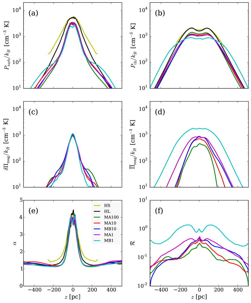
Figure 6: Temporally and horizontally averaged vertical profiles of (a) $P_{\rm turb}$, (b) $P_{\rm th}$, (c) $\delta\Pi_{\rm mag}$, (d) $\overline{\Pi}_{\rm mag}$, (e) $\alpha\equiv(P_{\rm turb}+P_{\rm th})/P_{\rm th}$, and (f) $\mathcal{R}\equiv(\delta\Pi_{\rm mag}+\overline{\Pi}_{\rm mag})/(P_{\rm turb}+P_{\rm th})$.

Figure 6(a)-(d) plots vertical profiles of the four individual support terms averaged over $(t_{1},t_{2})$ and the horizontal direction. Panel (e) shows the ratio of the kinetic (turbulent + thermal) to the thermal term, $\alpha\equiv(P_{\rm turb}+P_{\rm th})/P_{\rm th}$; and panel (f) shows the ratio of total magnetic to kinetic term, $\mathcal{R}\equiv(\delta\Pi_{\rm mag}+\overline{\Pi}_{\rm mag})/(P_{\rm turb}+P_{\rm th})$.

First of all, Figure 6 confirms that Models HS and HL agree very well not only for the mean and midplane values, but also for the overall profiles. The periodic vertical boundary conditions in Model HS introduce a small anomaly near the vertical boundaries.

In the presence of magnetic support, the turbulent and thermal terms are both reduced. However, the relative contribution between turbulent and thermal terms remains similar (Figure 6(e)): $\alpha\sim 4$ within one scale height, decreasing to $\alpha\sim 1$ at high-$|z|$. This is an important consequence of self-regulation by star formation feedback, explained in the equilibrium theory (see Section 4.3). The turbulent magnetic support in all magnetized models converges to very similar profiles (Figure 6(c)), while the mean magnetic support still shows differences (Figure 6(d)), especially for two extreme cases (Models MA100 and MB1). For all models except MB1, Figure 6(f) shows that the midplane value $\mathcal{R}_{0}\sim$0.2-0.5, while $\mathcal{R}$ becomes very small at high-$|z|$; Model MB1 has $\mathcal{R}\sim 0.3-1$.

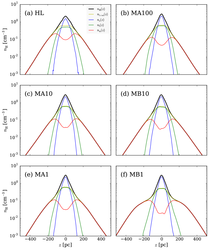
Figure 7: Vertical saturated-state density profiles of cold (blue; $T<184\;{\rm K}$), intermediate-temperature (green; $184\;{\rm K}<T<5050\;{\rm K}$), and warm (red; $T>5050\;{\rm K}$) gas phases. The profiles of total density (black) and combined non-cold phases (yellow; $T>184\;{\rm K}$) are also shown.

Figure 7 presents vertical profiles of the horizontally-averaged density from different thermal components of gas, for each model. We separately plot the profiles of cold ($n_{c}$; $T<184\;{\rm K}$), intermediate-temperature ($n_{i}$; $184\;{\rm K}<T<5050\;{\rm K}$), and warm ($n_{w}$; $T>5050\;{\rm K}$) phases, as well as the whole medium ($n_{H}=n_{c}+n_{i}+n_{w}$) and combined non-cold ($n_{i+w}$; $T>184\;{\rm K}$) components. The distribution of cold medium is mostly limited to one gas scale height, while the warm medium extends to high $|z|$ with a dip near the midplane. The intermediate temperature gas is not as concentrated toward the midplane as the cold medium, but does not extend to high $|z|$. Decomposition into cold ($n_{c}$) and non-cold ($n_{i+w}$) components gives two smooth profiles that resemble the results for two-component fits to observed H I gas from 21 cm emission.

Because most of cold medium resides within one gas scale height (and we do not consider runaway O stars), most of SN explosions occur there. The $P_{\rm turb}$ and $\alpha$ profiles in Figure 6 are peaked near the midplane, with scale heights similar to the cold medium scale height. The value of $\alpha$ is close to unity at $|z|>100$pc, implying that much of the turbulent energy dissipates very efficiently within the driving layer without propagating to high $|z|$. Thermal pressure is flat in the central layer, implying that the two-phase medium is well-mixed and in pressure equilibrium. Beyond the turbulent, two-phase layer, the ISM is mostly warm gas and is supported mainly by thermal pressure. Note that the shape of vertical profiles of the Reynolds and Maxwell stress are respectively similar to those of $P_{\rm turb}$ and $\delta\Pi_{\rm mag}$ (see Figure 6(a) and (c)).

In order to check vertical dynamical equilibrium quantitatively, for each model we calculate the weight of the gas using the horizontally and temporally averaged density and gravitational potentials, with $\mathcal{W}_{\rm sg}(z)$ and $\mathcal{W}_{\rm ext}(z)$ as in Equations (3) and (4) except integrated between $z$ and $z_{\rm max}$. Figure 8 plots the vertical profiles for the total support $\Delta P_{\rm tot}(z)={P_{\rm tot}}(z)-{P_{\rm tot}}(z_{\rm max})$ (blue) and the weight $\mathcal{W}(z)=\mathcal{W}_{\rm sg}(z)+\mathcal{W}_{\rm ext}(z)$ of the ISM (red). We also plot each component of the vertical support shown in Figure 8 along with the individual weights, to show the relative importance of the contributing terms in each model.

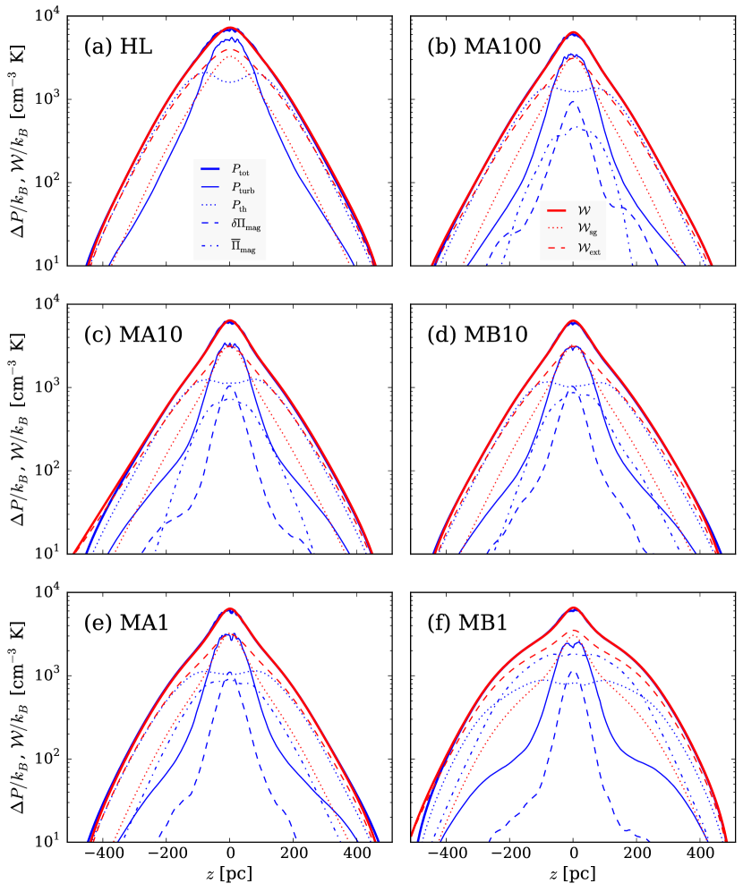
Figure 8: Profiles of saturated-state vertical support (blue) and gas weight (red). Total support and total weight are shown in thick lines. Thin blue solid, dotted, dashed, dot-dashed lines denote turbulent kinetic, thermal, turbulent magnetic, and mean magnetic support, respectively. Thin red dotted and dashed lines denote the weight of the ISM under self- and external gravity, respectively.

Figure 8 shows that vertical equilibrium is remarkably well satisfied (thick blue and red lines overlap almost completely). In the present simulations, the magnetic scale height is not very different from the gas scale height, especially for the turbulent component. Thus, similarly to the gas pressure terms we can simply replace $\Delta\Pi_{\rm mag}\rightarrow{\Pi_{\rm mag}}_{,0}$ in Equations (1) and (2). Since the weight of the gas (RHS of Eq. (5)) is more or less the same for all of the present models ($\chi\sim 1$ within 25% from Table 1), the additional support from both the mean and turbulent magnetic fields necessarily implies a reduction in the turbulent and thermal pressures compared to unmagnetized models. Although external gravity dominates the weight at high-$|z|$, self- and external gravity contributions are almost the same close to the midplane. Within the turbulent driving layer, turbulent pressure dominates other support terms for all models, while the thermal pressure dominates at high-$|z|$. The turbulent and mean magnetic support terms are as important as the thermal pressure at the midplane. Only for Model MB1, the mean magnetic support is substantial at all $z$. Table 3 includes the midplane values of the contribution to vertical support from each component.

4.3 Regulation of Star Formation Rates

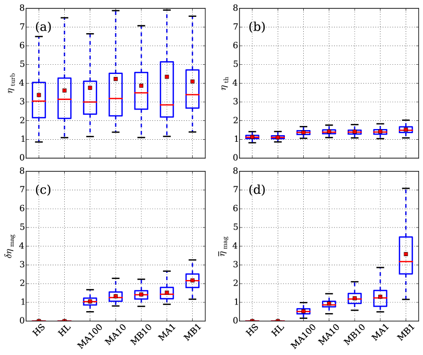
Figure 9: Feedback yields, defined in Equation (12): (a) $\eta_{\rm turb}$, (b) $\eta_{\rm th}$, (c) $\delta\eta_{\rm mag}$, and (d) $\overline{\eta}_{\rm mag}$. Box and whisker plot is as in Figure 3. Note that the mean (square symbol) and median (red line) of $\eta_{\rm turb}$ are different since the spikes in time evolution of $P_{\rm turb}$ (see Figure 5(a)) caused by SN feedback affect the mean more than the median.

We compute the feedback yield (ratio of midplane support to surface density of star formation rate) for each component at saturation, and report values in Table 3 in the units of Equation (12). These yields are a quantitative measure of the efficiency of feedback for controlling star formation. Figure 9 presents a box and whisker plot for each component feedback yield. As shown in Figure 9, the individual feedback yields except $\overline{\eta}_{\rm mag}$ are quite similar for all models. Notably, the magnetized models and unmagnetized models have comparable value for both turbulent and thermal feedback yields, $\eta_{\rm turb}\sim 3.5-4$ and $\eta_{\rm th}\sim 1.1-1.4$. The agreement of $\eta_{\rm turb}$ between HD and MHD models stems from the similarity in dissipation timescales for HD and MHD turbulence (e.g., Stone et al., 1998; Mac Low et al., 1998).

Except for models MA100 and MB1, the magnetic field and especially the turbulent magnetic energy become fairly well saturated, due to efficient generation from the small-scale turbulent dynamo. The resulting turbulent magnetic feedback yield for these models is $\delta\eta_{\rm mag}\sim 1.3-1.5$, providing a ratio $\eta_{\rm turb}/\delta\eta_{\rm mag}\sim 3-4$. This is equivalent to the energy ratios of $E_{\rm turb}/\delta E_{\rm mag}\sim(1.5-2)$ found in driven turbulence MHD simulations (e.g, Stone et al., 1998; Haugen et al., 2004; Cho et al., 2009; Lemaster & Stone, 2009). Table 3 includes $\overline{\eta}_{\rm mag}$ for reference. However, it should be kept in mind that the mean magnetic field support is less directly related to the SFR than the other terms. Mean magnetic fields arise from the mean-field dynamo, which depends on the turbulent magnetic field and therefore indirectly on the SFR, but also depends on other physical effects in a complex manner that is not well understood. From the present simulations, we simply note that $\overline{\eta}_{\rm mag}$ is comparable to $\delta\eta_{\rm mag}$ for the saturated models.

The theoretical idea of near-linear relationships between SFRs and turbulent and thermal pressures for self-regulated equilibrium ISM states was introduced and initially quantified by Ostriker et al. (2010); Ostriker & Shetty (2011); Kim et al. (2011). In the present simulations, our momentum feedback prescription for SNe injects radial momentum of $p_{*}=3\times 10^{5}\;{\rm M}_{\odot}\;{\rm km}\;{\rm s}^{-1}$ within a $10\;{\rm pc}$ sphere (see Paper I for details); other work confirms this value for the momentum from a single SN of energy $10^{51}\;{\rm erg}$, insensitive to the mean value of the ambient density or cloudy structure in the ambient ISM (see Kim & Ostriker, 2015, and references within). Our adopted value for the total mass of new stars formed per SN is $m_{*}=100\;{\rm M}_{\odot}$ (e.g. Kroupa, 2001). For these feedback parameters, the momentum flux/area in the vertical direction is then $P_{\rm driv}=(p_{*}/4m_{*})\Sigma_{\rm SFR}=3.6\times 10^{3}\Sigma_{\rm SFR,-3}k_{\rm B}\;{\rm cm}^{-3}\,{\rm K}$ (Ostriker & Shetty, 2011); this is the effective turbulent driving rate in the vertical direction. If dissipation of turbulence occurs in approximately a vertical crossing time over $H$ (the main energy-containing scale), the expected saturation level for turbulent pressure is ${P_{\rm turb}}_{,0}\approx P_{\rm driv}$, giving $\eta_{\rm turb}=3.6$. Direct calibration in Paper I gives ${P_{\rm turb}}_{,0}/P_{\rm driv}=1.20\Sigma_{\rm SFR,-3}^{-0.11}$ (see also Kim et al., 2011). Including results from both previous and current simulations, we obtain ${P_{\rm turb}}_{,0}/P_{\rm driv}=0.9$-$1.1$ from all HD and MHD models. Thus, the turbulent pressure is consistent with theoretical predictions, insensitive to magnetization.

As the SFR varies in our simulations, the time-varying heating rates move the thermal equilibrium curves up and down in the density-pressure phase plane. To maintain a two-phase medium within the midplane layer, the actual thermal pressure of gas must change to be self-consistent with the changing heating rate. Specifically, for a two-phase medium the range of the midplane thermal pressure is between the minimum and maximum pressures of the cold and warm medium, $P_{\rm min}$ and $P_{\rm max}$, respectively. Our adopted cooling and heating formalism gives ${P_{\rm min}}_{,3}=0.7\Sigma_{\rm SFR,-3}$ and ${P_{\rm max}}_{,3}=2.2\Sigma_{\rm SFR,-3}$ (see Koyama & Inutsuka, 2002; Kim et al., 2008). The geometric mean of these two pressures is representative of the expected thermal pressure in a two-phase medium (e.g., Wolfire et al., 1995, 2003), yielding ${P_{\rm two}}_{,3}\equiv({P_{\rm min}}_{,3}{P_{\rm max}}_{,3})^{1/2}=1.2\Sigma_{\rm SFR,-3}$. Ostriker et al. (2010) argued that the self-consistent expected midplane pressure for a star-forming disk in equilibrium is ${P_{\rm th}}_{,0}\sim P_{\rm two}$, corresponding to $\eta_{\rm th}=1.2$ for the thermal feedback yield. Here, we obtain ${P_{\rm th}}_{,0}/P_{\rm two}=1.0$-$1.3$ for all HD and MHD models, consistent with the theory in Ostriker et al. (2010), and with the numerical results in Paper I (see also Kim et al., 2011), ${P_{\rm th}}_{,0}/P_{\rm two}=1.09\Sigma_{\rm SFR,-3}^{-0.14}$.

In addition to the turbulent and thermal pressures, the turbulent magnetic support is also directly related to the SFR. As demonstrated in Figures 2 and 5, the small-scale turbulent dynamo generates turbulent magnetic fields efficiently. The turbulent magnetic energy is expect to saturate at roughly equipartition level with turbulent kinetic energy. In our simulations, the saturation level of turbulent magnetic energy is $\sim 40\%$ or slightly smaller compared to the turbulent kinetic energy (see Figure 3). If turbulent kinetic and magnetic components are all isotropic so that $P_{\rm turb}=(1/3)\rho|\delta\mathbf{v}|^{2}=(2/3)E_{\rm turb}$ and $\delta\Pi_{\rm mag}=(1/3)|\delta\mathbf{B}|^{2}/8\pi=(1/3)\delta E_{\rm mag}$, then $E_{\rm turb}\sim 2\delta E_{\rm mag}$ (Figure 3) would give $P_{\rm turb}\sim 4\delta\Pi_{\rm mag}$. We find ${P_{\rm turb}}_{,0}\sim P_{\rm driv}\sim 3{\delta\Pi_{\rm mag}}_{,0}$, except for Model MB1, see Table 3. In idealized, driven MHD turbulence simulations, $E_{\rm turb}/\delta E_{\rm mag}\sim 1-2.5$ for various initial magnetic fields, Mach number, and compressibility of gas (e.g., Haugen et al., 2004; Cho et al., 2009; Lemaster & Stone, 2009). Our simulations are generally consistent with saturation energy levels from idealized driven turbulence experiments in a periodic box, keeping in mind that identical results are not expected considering differences in the setup. (That is, rather than an idealized periodic box with spectral driving of turbulence, our simulations incorporate complex physics to model realistic galactic disks including vertical stratification, compressibility, spatially localized turbulent driving, self-consistent evolution of mean fields, self-gravity, presence of cooling and heating, and so on.)

Our simulations are suggestive, but not conclusive, with respect to the asymptotic equilibrium state of the mean magnetic support and its connection to SFRs. The mean fields for all models appear to be converging to the same level of support as the turbulent fields (e.g., as in Model MB10; see Figure 1), which as shown above have ${\delta\Pi_{\rm mag}}\propto\Sigma_{\rm SFR}$. Note that the mean magnetic field is anisotropic and dominated by the azimuthal component, so $\overline{\Pi}_{\rm mag}=\overline{E}_{\rm mag}$ in contrast to $\delta\Pi_{\rm mag}=(1/3)\delta E_{\rm mag}$ for the isotropic case. However, longer-term simulations would be needed to confirm convergence of $\overline{\Pi}_{\rm mag}$, because the evolution time scale for the mean field is much longer than for the turbulent field (see Figure 2). In addition, the mean field level may in principle be affected by numerical parameters including the horizontal box size and effective numerical resistivity. Thus, it remains uncertain whether the mean magnetic support should be considered as directly related to the SFR or not. Models MA10, MB10, and MA1 appear closest to saturation in their mean magnetic field, and have ${\overline{\Pi}_{\rm mag}}_{,0}/P_{\rm driv}\sim 0.3$, which would correspond to $\overline{\eta}_{\rm mag}\sim 1$. For reference, Models MA100 and MB1 respectively have ${\overline{\Pi}_{\rm mag}}_{,0}/P_{\rm driv}\sim 0.14$ and 0.9, although with the caveat that these models are not asymptotically converged.

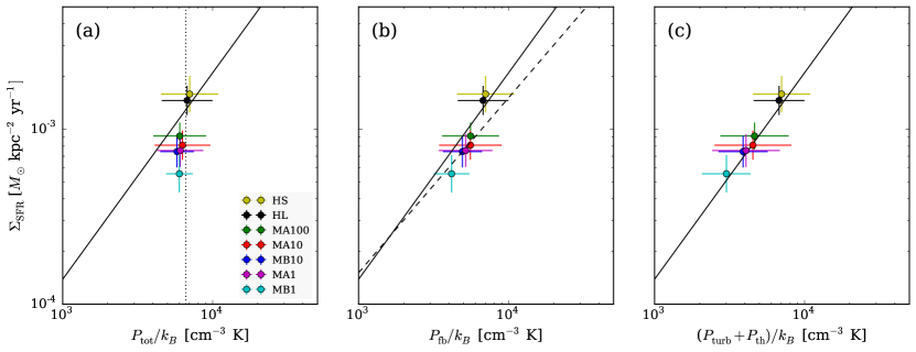
Figure 10: The SFR surface density as a function of midplane values of the effective pressure, (a) total pressure $P_{\rm tot}\equiv P_{\rm turb}+P_{\rm th}+\delta\Pi_{\rm mag}+\overline{\Pi}_{\rm mag}$, (b) feedback pressure $P_{\rm fb}\equiv P_{\rm turb}+P_{\rm th}+\delta\Pi_{\rm mag}$, and (c) kinetic pressure $P_{\rm turb}+P_{\rm th}$. The solid line denotes the fit from a wide parameter space of HD models in Paper I (see text). The vertical dotted line in (a) is the midplane pressure required for the vertical dynamical equilibrium, $P_{\rm tot,DE}=\pi G\Sigma^{2}(1+\chi)/2=6.6\times 10^{3}k_{\rm B}\;{\rm cm}^{-3}\,{\rm K}$ for $\chi=1$. The dashed line in (b) is the relationship between $\Sigma_{\rm SFR}$ and $P_{\rm fb}$ using Equation (12) with total feedback yield for the fiducial run, MB10, $\eta_{\rm turb}+\eta_{\rm th}+\delta\eta_{\rm mag}=6.6$.

Figure 10 plots $\Sigma_{\rm SFR}$ as functions of three midplane (effective) pressures, (a) total pressure ${P_{\rm tot}}\equiv{P_{\rm turb}}+{P_{\rm th}}+{\delta\Pi_{\rm mag}}+{\overline{\Pi}_{\rm mag}}$, (b) total “feedback” pressure ${P_{\rm fb}}\equiv{P_{\rm turb}}+{P_{\rm th}}+{\delta\Pi_{\rm mag}}$, and (c) kinetic pressure ${P_{\rm turb}}+{P_{\rm th}}$. We also plot as a solid line the fitting result from HD models in Paper I for a wide range of $\Sigma$ and $\rho_{\rm sd}$, $\Sigma_{\rm SFR,-3}=2.1[{(P_{\rm turb}+P_{\rm th})}/10^{4}k_{\rm B}\;{\rm cm}^{-3}\,{\rm K})]^{1.18}$. The vertical dotted line in panel (a) denotes the total ISM weight when $\chi=1$ (as in Table 1), $P_{\rm tot,DE}=\mathcal{W}_{0}=\pi G\Sigma^{2}(1+\chi)/2\rightarrow 6.6\times 10^{3}k_{\rm B}\;{\rm cm}^{-3}\,{\rm K}$. As shown in Figure 8, vertical dynamical equilibrium indeed holds so that the total midplane pressure adjusts to match this weight. We note that the total midplane pressure and weight are very similar for all models ($\chi\sim 1$ agrees within 25% for all cases), since we fix $\Sigma$ and $\rho_{\rm sd}$, and $\sigma_{\mathrm{eff}}$ and $\zeta_{d}$ are insensitive to the model parameters. The vertically aligned symbols in Figure 10(a) show graphically the consistency of ${P_{\rm tot}}_{,0}$ and $\mathcal{W}_{0}$ in all models, and also make clear that the inclusion of magnetic terms reduces $\Sigma_{\rm SFR}$ for the same ${P_{\rm tot}}_{,0}$.

Since the mean magnetic field can supply vertical support without star formation (at least on timescales comparable to the disk’s vertical crossing time), the total support requirement from star formation feedback for the vertical equilibrium can be reduced to ${P_{\rm fb}}=P_{\rm tot,DE}-{\Delta\overline{\Pi}_{\rm mag}}$ (where we assume $\delta\Pi_{\rm mag}(z_{\rm max})\rightarrow 0$, as turbulent fields are driven only within the star-forming layer, but we keep $\overline{\Pi}_{\rm mag}(z_{\rm max})$ for generality, allowing for the possibility that the mean fields are carried into the halo by winds). Thus, it is interesting to plot $\Sigma_{\rm SFR}$ as a function of midplane values of ${P_{\rm fb}}$ instead of ${P_{\rm tot}}$, which we show in Figure 10(b). In the presence of magnetic fields, even with very weak mean fields, star formation feedback can generate turbulent magnetic fields at a significant level in a very short time. The additional support from turbulent magnetic fields enhances overall feedback yield with $\delta\eta_{\rm mag}\sim 1-2$ on top of $\eta_{\rm turb}+\eta_{\rm th}\sim 4-5$. Thus, the feedback pressure is larger by 20%-40% at a given SFR for a magnetized medium compared to an unmagnetized medium. The dashed line in panel (b) represents $\Sigma_{\rm SFR,-3}={P_{\rm fb}}_{,3}/(\eta_{\rm turb}+\eta_{\rm th}+\delta\eta_{\rm mag})$ with $\eta_{\rm turb}+\eta_{\rm th}+\delta\eta_{\rm mag}=6.6$, the feedback yield for Model MB10. As expected, the symbols and the dashed line in Figure 10(b) for magnetized models fall systematically below (or to the right) of the solid line, which was based on simulation results from HD models with lower total $\eta$ than MHD models.

Figure 10(c) shows another important property of self-regulated star-forming ISM disks. Since $\eta_{\rm turb}$ and $\eta_{\rm th}$ are nearly unchanged with and without magnetic fields, the same relationship between kinetic midplane pressure ${P_{\rm turb}+P_{\rm th}}$ and SFR holds as we found in Paper I (solid line). However, the present work considers only a single value of $\Sigma$ and $\rho_{\rm sd}$, and simulations for a wider range of these parameters, for magnetized models, would be needed to confirm the robustness of this conclusion.

In short, the presence of the magnetic fields will reduce the SFR by increasing the total efficiency of feedback ($\eta_{\rm turb}+\eta_{\rm th}+\delta\eta_{\rm mag}$) and reducing the required dynamical equilibrium pressure from feedback ($P_{\rm tot,DE}-\Delta{\overline{\Pi}_{\rm mag}}$). The general relationship between the SFR surface density and the midplane pressure including magnetic terms can then be written as

$$\Sigma_{\rm SFR}=10^{-3}\;{\rm M}_{\odot}\;{\rm kpc}^{-2}\;{\rm yr}^{-1}\left({\frac{\eta_{\rm turb}+\eta_{\rm th}+\delta\eta_{\rm mag}}{5}}\right)^{-1}\left({\frac{P_{\rm tot,DE}-{\Delta\overline{\Pi}_{\rm mag}}}{5\times 10^{3}k_{\rm B}\;{\rm cm}^{-3}\,{\rm K}}}\right).$$ (17)

If $\Delta\overline{\Pi}_{\rm mag}$ is asymptotically proportional to $\Sigma_{\rm SFR}$ (which would be true if the mean-field dynamo arises from feedback-driven fluctuations in the magnetic and velocity fields, similar to the small-scale turbulent dynamo), a relationship of the form $\Sigma_{\rm SFR}\propto P_{\rm tot,DE}$ with larger total efficiency of feedback would also hold. Alternatively, $\Delta\overline{\Pi}_{\rm mag}$ may be negligible compared to $P_{\rm tot,DE}$ if the scale height of the mean magnetic field is large compared to that of the neutral ISM.

5 Summary and Discussion

In Paper I, we developed realistic galactic disk models with cooling and heating, self-gravity, sheared galactic rotation, and self-consistent star formation feedback using direct momentum injection by SNe and time-varying heating rates. Here, we extend the fiducial Solar-neighborhood-like model of Paper I to include magnetic fields with varying initial field strengths and distributions. We also alter the initial and boundary conditions from the original model to minimize artificial initial vertical oscillations. We show in Section 4.1 that the overall evolution remains the same in HD models irrespective of differences in initial and boundary conditions, confirming the robustness of results in Paper I. In both HD and MHD models, the time evolution of ISM properties reaches a saturated equilibrium state within $\sim t_{\rm orb}$, except for the mean magnetic field, which continues to secularly evolve over several $t_{\rm orb}$ (see Figures 1 and 2). In what follows, we summarize the main results derived from analyzing the time evolution of mean ISM properties and final saturated-state vertical profiles, with careful consideration of the slow variation of mean magnetic fields.

1. Generation and Saturation of Magnetic Fields – Turbulent motions in our simulations quickly develop and saturate. The same is true for turbulent magnetic fields (see Figure 2(b)). Beyond $\sim t_{\rm orb}$, saturated levels of turbulent kinetic and magnetic energies are similar for all MHD models except Model MA100, which has a very weak initial field. Model MA100 converges to the same levels of $E_{\rm turb}$ and $\delta E_{\rm mag}$ as other models by $\sim 3t_{\rm orb}$. The final saturated state has mass-weighted mean $\langle\delta{v}^{2}\rangle_{M}^{1/2}\approx 5\;{\rm km}\;{\rm s}^{-1}$ and $\langle\delta{v}_{A}^{2}\rangle_{M}^{1/2}\approx 3\;{\rm km}\;{\rm s}^{-1}$ for all MHD models, corresponding to $E_{\rm turb}/\delta E_{\rm mag}\sim 2.5$.

   The growth of magnetic fields in turbulent flows is believed to be a consequence of turbulent dynamo action, which generally refers to mechanisms of energy conversion from kinetic to magnetic. Dynamos are classified into large-scale (mean field) dynamos and small-scale (fluctuation or turbulent) dynamos. The former and latter respectively generate magnetic fields with scales larger and smaller than the turbulence injection scale. In many spiral galaxies, there are significant large-scale, regular azimuthal magnetic fields (e.g., Beck, 2001), which may result from the so-called $\alpha-\Omega$ dynamo driven by turbulence and differential rotation (e.g., Beck et al., 1996). Our initial conditions with mean fields in the $\hat{\mathbf{y}}$ direction is motivated by observed preferentially azimuthal (or spiral-arm aligned) fields. Self-consistent growth of mean fields from the very weak primordial magnetic fields is an important and active research area (see Gressel et al., 2008; Gent et al., 2013b, for recent simulations with SN). Although growth of mean magnetic fields is not the main focus of this paper, some hints can be found in the evolution of mean fields in cases with initially weak fields (Models MA100 and MA10 in Figure 2(d)).

   More straightforward results from our simulations are the saturation properties of turbulent magnetic fields, which can be understood in the context of small-scale dynamos. It is broadly known that turbulent conductive flows can amplify their own magnetic fields through random field line stretching, twisting, and folding (e.g., Zeldovich et al., 1983; Brandenburg & Subramanian, 2005). Recently, Cho et al. (2009) have quantified three stages of evolution using a comprehensive set of nonlinear simulations for incompressible MHD turbulence (see also Schekochihin & Cowley, 2007; Beresnyak, 2012). The magnetic energy grows exponentially until it reaches equipartition at the kinetic energy dissipation scale. Then, growth becomes linear until the entire energy spectrum reaches equipartition up to the energy injection scale. The saturation amplitude of turbulent magnetic energy for small-scale incompressible dynamos approaches $\sim 40\%$ of the total energy at large Reynolds number (Cho et al., 2009). Haugen et al. (2004) obtained $\sim 30\%$ of the total energy from their compressible simulations. Lemaster & Stone (2009) obtained similar results for various Mach numbers from isothermal, compressible MHD simulations (see also Ryu et al., 2008). Nearly irrespective of the Mach number, the ratios of magnetic energy to total (kinetic+magnetic) energy in fluctuations are $30-40\%$. With stronger initial field, saturation is achieved more rapidly.

   The small-scale dynamo provides a fast and universal mechanism for magnetic field amplification (Brandenburg & Subramanian, 2005; Beresnyak & Lazarian, 2015). Thus, we expect that qualitatively similar processes will occur in our simulations in spite of their greater physical complexity, including compressibility, vertical stratification, SN driven turbulence, self-gravity, and multiphase gas with cooling and heating. In early phases $t<t_{\rm orb}$, rapid growth and saturation of the turbulent magnetic energy are induced by driven turbulence (see Figure 2). After $t_{\rm orb}$, turbulence is driven entirely by SN feedback, with a rate that depends on the SFR. Vertical dynamical equilibrium (see below) dictates the turbulent pressure level, and hence SFR, that is self-consistently reached in these disk systems. The final saturated-state turbulent magnetic energy level is about half of turbulent kinetic energy, as expected in small-scale dynamo simulations.

2. Vertical Structure of the Diffuse ISM – The vertical distribution and gravitational support of the diffuse ISM in the Milky Way has been investigated many times under the assumption of vertical dynamical equilibrium (Boulares & Cox, 1990; Lockman & Gehman, 1991; Kalberla & Kerp, 1998). In Section 4.2, we validate that vertical dynamical equilibrium is satisfied in turbulent, star-forming, magnetized galactic disks, extending results from previous multiphase ISM simulations with various physical ingredients (Piontek & Ostriker, 2007; Koyama & Ostriker, 2009; Kim et al., 2010, 2011, 2013; Hill et al., 2012). At the midplane, vertical support is dominated by the turbulent (kinetic) pressure except in model (MB1) with very strong mean magnetic fields (see Figure 8 and Table 3). Thermal and turbulent magnetic supports are comparable to each other and about 2-3 times smaller than the turbulent pressure. Compared to HD models, MHD disk models can maintain smaller turbulent and thermal pressures owing to additional vertical support from the turbulent and mean magnetic fields. Despite of different magnetization, the total effective velocity dispersion $\sigma_{\mathrm{eff}}$ varies by only $\sim 25\%$ over all models (see Table 2), resulting in similar variation in $\chi$ and hence dynamical equilibrium midplane pressure $P_{\rm tot,DE}=\mathcal{W}_{0}={\mathcal{W}_{\rm sg}}_{,0}(1+\chi)$.

   Our models demonstrate that vertical dynamical equilibrium is indeed a good assumption even though disks are magnetized and highly dynamic. However, practical application of vertical equilibrium in observations is not simple. Even in the Solar neighborhood, uncertainty is substantial. For example, Boulares & Cox (1990) calculated the total equilibrium pressure based on observations of the vertical gas distribution and gravity (e.g., Bienayme et al., 1987; Kuijken & Gilmore, 1989), and taking the difference with observed thermal+turbulent pressure inferred significant contributions from non-thermal (cosmic-ray and magnetic) pressures. However, Lockman & Gehman (1991) have argued that local (high-latitude) H I 21 cm emission data can be fitted with three-component Gaussians, and that non-thermal vertical support is not necessary to explain the H I distribution. Considering the large observed scale height of non-thermal pressure terms, the vertical support of H I within $|z|<1\;{\rm kpc}$ (which depends on the pressure gradient, not pressure itself), can be explained solely by thermal + turbulent terms. Later, Kalberla & Kerp (1998) simultaneously analysed the distribution of emission at 21 cm from warm/cold H I with H$\alpha$ from diffuse ionized gas, soft X-rays for the hot medium, and synchrotron radiation combined with $\gamma$-ray emission probing magnetic fields and cosmic rays. They concluded that within $400\;{\rm pc}$ of the midplane, cosmic ray support is not required, and turbulent magnetic fields contribute with $\mathcal{R}\sim 1/3$ ($\alpha=1/3$ in their notation). The contribution of turbulent magnetic support compared to thermal+turbulent kinetic pressure in our simulations is $\sim 25\%$ from Table 3, in good agreement with this result. In our simulations, the mean magnetic field has a relatively small scale height (Figure 6) and vertical support slightly less than that of the turbulent magnetic field. In contrast, observations indicate that magnetic fields extend into the halo in equipartion with the pressures of cosmic rays and hot gas. The decline in mean magnetic fields with height in our present simulations may be due to the absence of a hot medium and cosmic rays; this issue will be addressed in future work.

   Adoption of vertical equilibrium is useful to estimate the midplane pressure in external galaxies. The pressure cannot be measured directly except for nearby edge-on disks, and even in that case requires deprojection and an assumption for the turbulent velocity dispersion (Yim et al., 2011, 2014). As outlined in Section 2, to get the total dynamical equilibrium pressure (or the total weight of the gas; see Equation (5)), one may need to determine $\Sigma$, $\Sigma_{*}$, $\sigma_{*}$, and $\sigma_{\mathrm{eff}}$ (or $\sigma_{z}$ and $\mathcal{R}$), assuming the parameter $\zeta_{d}\sim 0.4-0.5$ is nearly constant. In several systematic studies of nearby galaxies (Blitz & Rosolowsky, 2004, 2006; Leroy et al., 2008; Kasparova & Zasov, 2008), $\sigma_{\mathrm{eff}}$ and/or $H_{*}\propto\sigma_{*}^{2}/\Sigma_{*}$ are assumed to be constant to determine the total midplane pressure. Observational measurements have suggested that H I velocity dispersions are nearly constant with $\sigma_{z}\sim 5-10\;{\rm km}\;{\rm s}^{-1}$, especially for the atomic gas dominated regime, using single Gaussian fitting (Petric & Rupen, 2007) and intensity-weighted second velocity moments (Tamburro et al., 2009). Recent studies of global H I kinematics analysis to obtain “superprofiles” (averaged H I profiles for the entire galaxy) in nearby spiral and dwarf galaxies have arrived at similar conclusions (Stilp et al., 2013; Ianjamasimanana et al., 2012). In this paper, we show that the contribution from turbulent magnetic field to $\mathcal{R}$ (or, equivalently, $[\delta{v}_{A}^{2}/2-\delta v_{A,z}^{2}]/\sigma_{z}^{2})$ is $\approx 0.3$ insensitive to the mean magnetic field strength for saturated models (except Model MB1). This suggests that if the total velocity dispersion $\sigma_{z}$ can be measured accurately, an estimate of $\sigma_{\mathrm{eff}}$ needed to compute $C$ and $\chi$ and therefore the total midplane pressure may be obtained using a typical value of $\mathcal{R}\sim 0.3$ even if the observed magnetic field strength is not measured.

   The density structure in our simulations is well characterized by two components, a cold and non-cold medium (see Figure 7). For the present models, we find scale heights of cold and non-cold components are $H\sim 30\;{\rm pc}$ and $110\;{\rm pc}$, respectively. Lockman & Gehman (1991) have used three-component Gaussians to fit H I emission line observations near the Sun, obtaining vertical scale heights equivalent to $H\sim 80-130\;{\rm pc}$, $\sim 150-300\;{\rm pc}$, and $\sim 600-750\;{\rm kpc}$ (see also Dickey & Lockman, 1990). A recent Herschel galactic survey of [C II], along with ancillary H I, ¹²CO, ¹³CO, and C¹⁸O data, shows that the equivalent vertical scale heights of [C II] sources with CO and without CO which trace colder/denser vs. warmer/more diffuse gas, respectively, are $\sim 70\;{\rm pc}$ and $170\;{\rm pc}$ (Langer et al., 2014; Velusamy & Langer, 2014). Our simulations agree with both of these observational studies in the sense that the warmer component has $\sim 2-3$ times the scale height of the colder component. However, our measured $H$ values are somewhat lower than observed Solar-neighborhood values, as our measured values of $\sigma_{z}$ and $\Sigma_{\rm SFR}$. Simulations currently underway that include a hot ISM suggest that $H$, $\sigma_{z}$, and $\Sigma_{\rm SFR}$ may increase.

3. Feedback Efficiencies and Star Formation Laws – One of the important conclusions of this study is that the feedback yields for turbulent and thermal pressure are unchanged by the presence of magnetic fields. This is mainly because the HD and MHD turbulent energy dissipation rates are similar. The dissipation time scale is always of order the crossing time at the driving scale (or main energy-containing scale) both for HD turbulence (Kaneda et al., 2003) and MHD turbulence (Stone et al., 1998; Mac Low et al., 1998; Lemaster & Stone, 2009; Cho et al., 2009), and both compressible and incompressible flows. Turbulent magnetic fields saturate at a similar timescale to turbulent velocities. Balancing turbulent driving with turbulent dissipation therefore leads to direct proportionality between $\Sigma_{\rm SFR}$ and the turbulent kinetic and magnetic pressures. Similarly, balancing heating and cooling leads to a direct proportionality between $\Sigma_{\rm SFR}$ and the thermal pressure. turbulent kinetic and magnetic pressures. Defining “yield” as the pressure-to-$\Sigma_{\rm SFR}$ ratio (in convenient units; see Equation 12), we obtain turbulent, thermal, and turbulent magnetic feedback yields as $\eta_{\rm turb}\sim 3.5-4$, $\eta_{\rm th}\sim 1.1-1.4$, and $\delta\eta_{\rm mag}\sim 1.3-1.5$, respectively. Since the ISM weight and therefore total pressure is nearly the same irrespective of magnetization, the addition of magnetic terms to the total $\eta$ reduces $\Sigma_{\rm SFR}$ for MHD compared to HD simulations at a given $\Sigma$ and $\rho_{\rm sd}$.

   Correlations between the estimated ISM equilibrum pressure $P_{\rm tot,DE}$ and the molecular content and star formation rate have been identified empirically (e.g., Wong & Blitz, 2002; Blitz & Rosolowsky, 2006; Leroy et al., 2008). In particular, the $P-\Sigma_{\rm SFR}$ relation has much less scatter than the classical Kennicutt-Schmidt relationship (Kennicutt & Evans, 2012) between gas surface density $\Sigma$ and $\Sigma_{\rm SFR}$ for the atomic-dominated regime (e.g. Bigiel et al., 2008, 2010). As argued in our previous work (e.g., Ostriker et al., 2010; Kim et al., 2011, Paper I), this is because the total midplane pressure is directly related to the SFR, whereas ISM properties (and the SFR) can vary considerably at a given value of $\Sigma$ depending on the gravitational potential confining the disk. As shown in Ostriker & Shetty (2011, see also ), in the starburst regime where self-gravity dominates the potential, both pressure and surface density correlate well with SFR surface density, giving $\Sigma_{\rm SFR}\propto P_{\rm tot,DE}\propto\Sigma^{2}$ (shallower reported slopes are arguably due to too-high assumed CO-to-H₂ ratios at high $\Sigma$; see Narayanan et al. 2012). In the atomic-dominated regime, as modelled in this paper, the dynamical equilibrium pressure depends on both $\mathcal{W}_{\rm sg}\propto\Sigma^{2}$ and $\mathcal{W}_{\rm ext}\propto\Sigma\sqrt{\rho_{\rm sd}}$ (see Equations (3) and (4)). In outer disks where $\rho_{\rm sd}$ varies more than $\Sigma_{\mathrm{atomic}}\sim 6-10\;{\rm M}_{\odot}\;{\rm pc}^{-2}$, simple Kennicutt-Schmidt laws fail.

   As demonstrated in this paper, there can also be scatter introduced in $\Sigma_{\rm SFR}$ vs. $P_{\rm tot,DE}$ if support from the mean magnetic field contributes substantially without itself having $\Delta\overline{\Pi}_{\rm mag}\propto\Sigma_{\rm SFR}$. Even if a mean-field dynamo secularly leads to a well-define asymptotic ratio between $\Delta\overline{\Pi}_{\rm mag}$ and $\Sigma_{\rm SFR}$, the long timescale to reach this may mean that $\Delta\overline{\Pi}_{\rm mag}$ is not well correlated with the recent SFR. If the vertical scale height of the mean field is larger than that of the star-forming gas, however, the support from $\Delta\overline{\Pi}_{\rm mag}$ would be small even if the mean field pressure is non-negligible, which would reduce scatter in $\Sigma_{\rm SFR}$ vs. $P_{\rm tot,DE}$.

Appendix A Numerical Convergence

We adopt a standard spatial resolution of $\Delta=$2pc throughout this paper. Here, we present a convergence study for physical properties at the saturated state. Since a simulation with $\Delta=$1pc for the same box size would be too computationally expensive for our current facilities, we instead have rerun Model MB10 with $\Delta=$1pc, 2pc, and 4pc using a smaller horizontal box ($L_{x}=L_{y}=256\;{\rm pc}$) and a halved the turbulence driving period ($t_{\rm drive}=0.5t_{\rm orb}$) and final time ($t_{\rm end}=2t_{\rm orb}$).

Figure 11 summarizes the midplane support components and the energy ratios for $(t_{\rm orb},2t_{\rm orb})$ with box-and-whisker plots. We plot the quantities by taking the logarithms for clearer presentation of temporal fluctuations. We label the original MB10 model (full box with $\Delta=2pc$) as ‘MB10’ and the smaller box counterparts at three different resolutions as ‘1pc’, ‘2pc’, and ‘4pc’. Although the smaller box increases temporal fluctuations as expected, all components except the mean magnetic component show statistically converged results.

The mean magnetic component in the 1pc simulation is systematically reduced, and has the largest temporal fluctuation, also causing a slightly smaller saturated value of the turbulent magnetic component. Considering that the mean magnetic component always shows the slowest convergence, it is possible that with a longer integration time, the mean magnetic field in the 1pc model would approach that of the other models. However, it is also possible that it would remain at this reduced level. Since the evolution of mean magnetic fields is not the main focus of this paper, we defer further study of the mean magnetic component to future work, which will include more comprehensive investigation of mean field dynamo.

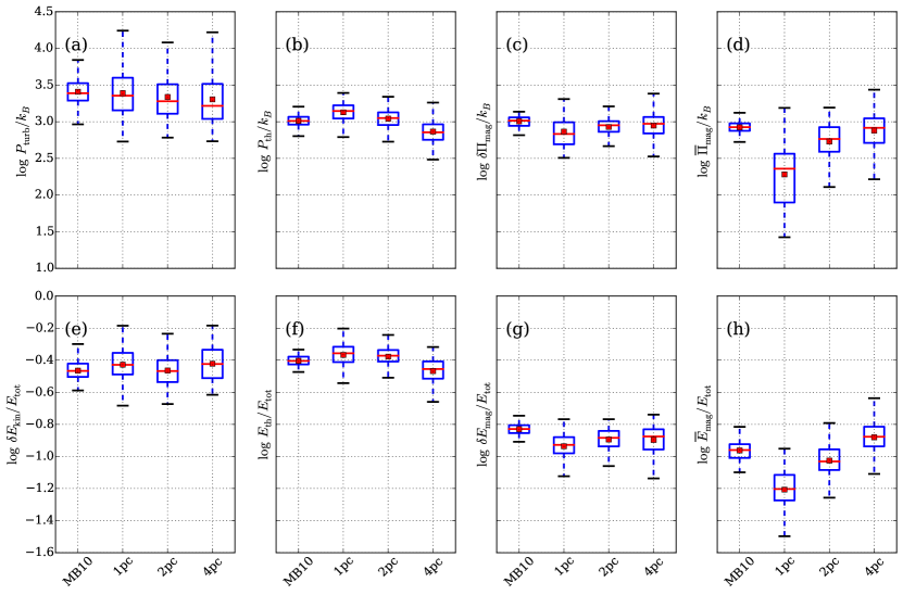
Figure 11: Box and whisker plots of the logarithms of the midplane support components (top; (a)-(d)) and the energy ratios (bottom; (e)-(h)) over the interval $(t_{\rm orb},2t_{\rm orb})$. From left to right columns, we show the turbulent kinetic, thermal, turbulent magnetic, and mean magnetic components. We label the original MB10 model as ‘MB10’, while the smaller box counterparts at three different resolutions are labeled ‘1pc’, ‘2pc’, and ‘4pc’.

References

- Beck (2001) Beck, R. 2001, Space Sci. Rev., 99, 243
- Beck et al. (1996) Beck, R., Brandenburg, A., Moss, D., Shukurov, A., & Sokoloff, D. 1996, ARA&A, 34, 155
- Beresnyak (2012) Beresnyak, A. 2012, Physical Review Letters, 108, 035002
- Beresnyak & Lazarian (2015) Beresnyak, A., & Lazarian, A. 2015, in Astrophysics and Space Science Library, Vol. 407, Astrophysics and Space Science Library, ed. A. Lazarian, E. M. de Gouveia Dal Pino, & C. Melioli, 163
- Bienayme et al. (1987) Bienayme, O., Robin, A. C., & Creze, M. 1987, A&A, 180, 94
- Bigiel et al. (2010) Bigiel, F., Leroy, A., Walter, F., et al. 2010, AJ, 140, 1194
- Bigiel et al. (2008) —. 2008, AJ, 136, 2846
- Blitz & Rosolowsky (2004) Blitz, L., & Rosolowsky, E. 2004, ApJ, 612, L29
- Blitz & Rosolowsky (2006) —. 2006, ApJ, 650, 933
- Boulares & Cox (1990) Boulares, A., & Cox, D. P. 1990, ApJ, 365, 544
- Brandenburg & Subramanian (2005) Brandenburg, A., & Subramanian, K. 2005, Phys. Rep., 417, 1
- Cho et al. (2009) Cho, J., Vishniac, E. T., Beresnyak, A., Lazarian, A., & Ryu, D. 2009, ApJ, 693, 1449
- Cox & Smith (1974) Cox, D. P., & Smith, B. W. 1974, ApJ, 189, L105
- Creasey et al. (2013) Creasey, P., Theuns, T., & Bower, R. G. 2013, MNRAS, 429, 1922
- de Avillez & Breitschwerdt (2004) de Avillez, M. A., & Breitschwerdt, D. 2004, A&A, 425, 899
- de Avillez & Breitschwerdt (2005) —. 2005, A&A, 436, 585
- Dickey & Lockman (1990) Dickey, J. M., & Lockman, F. J. 1990, ARA&A, 28, 215
- Dickey et al. (2009) Dickey, J. M., Strasser, S., Gaensler, B. M., et al. 2009, ApJ, 693, 1250
- Elmegreen & Scalo (2004) Elmegreen, B. G., & Scalo, J. 2004, ARA&A, 42, 211
- Federrath et al. (2011) Federrath, C., Chabrier, G., Schober, J., et al. 2011, Physical Review Letters, 107, 114504
- Ferrière (2001) Ferrière, K. M. 2001, Reviews of Modern Physics, 73, 1031
- Field (1965) Field, G. B. 1965, ApJ, 142, 531
- Field et al. (1969) Field, G. B., Goldsmith, D. W., & Habing, H. J. 1969, ApJ, 155, L149
- Gent et al. (2013a) Gent, F. A., Shukurov, A., Fletcher, A., Sarson, G. R., & Mantere, M. J. 2013a, MNRAS, 432, 1396
- Gent et al. (2013b) Gent, F. A., Shukurov, A., Sarson, G. R., Fletcher, A., & Mantere, M. J. 2013b, MNRAS, 430, L40
- Gressel et al. (2008) Gressel, O., Elstner, D., Ziegler, U., & Rüdiger, G. 2008, A&A, 486, L35
- Haugen et al. (2004) Haugen, N. E., Brandenburg, A., & Dobler, W. 2004, Phys. Rev. E, 70, 016308
- Haverkorn (2015) Haverkorn, M. 2015, in Astrophysics and Space Science Library, Vol. 407, Astrophysics and Space Science Library, ed. A. Lazarian, E. M. de Gouveia Dal Pino, & C. Melioli, 483
- Hawley et al. (1995) Hawley, J. F., Gammie, C. F., & Balbus, S. A. 1995, ApJ, 440, 742
- Heiles & Troland (2003) Heiles, C., & Troland, T. H. 2003, ApJ, 586, 1067
- Heiles & Troland (2005) —. 2005, ApJ, 624, 773
- Hennebelle & Iffrig (2014) Hennebelle, P., & Iffrig, O. 2014, A&A, 570, A81
- Hill et al. (2012) Hill, A. S., Joung, M. R., Mac Low, M.-M., et al. 2012, ApJ, 750, 104
- Ianjamasimanana et al. (2012) Ianjamasimanana, R., de Blok, W. J. G., Walter, F., & Heald, G. H. 2012, AJ, 144, 96
- Jenkins & Tripp (2011) Jenkins, E. B., & Tripp, T. M. 2011, ApJ, 734, 65
- Joung & Mac Low (2006) Joung, M. K. R., & Mac Low, M.-M. 2006, ApJ, 653, 1266
- Joung et al. (2009) Joung, M. R., Mac Low, M.-M., & Bryan, G. L. 2009, ApJ, 704, 137
- Kalberla & Kerp (1998) Kalberla, P. M. W., & Kerp, J. 1998, A&A, 339, 745
- Kaneda et al. (2003) Kaneda, Y., Ishihara, T., Yokokawa, M., Itakura, K., & Uno, A. 2003, Physics of Fluids, 15, L21
- Kasparova & Zasov (2008) Kasparova, A. V., & Zasov, A. V. 2008, Astronomy Letters, 34, 152
- Kennicutt & Evans (2012) Kennicutt, R. C., & Evans, N. J. 2012, ARA&A, 50, 531
- Kim et al. (2008) Kim, C.-G., Kim, W.-T., & Ostriker, E. C. 2008, ApJ, 681, 1148
- Kim et al. (2010) —. 2010, ApJ, 720, 1454
- Kim et al. (2011) —. 2011, ApJ, 743, 25
- Kim & Ostriker (2015) Kim, C.-G., & Ostriker, E. C. 2015, ApJ, 802, 99
- Kim et al. (2013) Kim, C.-G., Ostriker, E. C., & Kim, W.-T. 2013, ApJ, 776, 1
- Kim et al. (2014) —. 2014, ApJ, 786, 64
- Kim et al. (2003) Kim, W.-T., Ostriker, E. C., & Stone, J. M. 2003, ApJ, 599, 1157
- Koyama & Inutsuka (2002) Koyama, H., & Inutsuka, S.-i. 2002, ApJ, 564, L97
- Koyama & Ostriker (2009) Koyama, H., & Ostriker, E. C. 2009, ApJ, 693, 1346
- Kroupa (2001) Kroupa, P. 2001, MNRAS, 322, 231
- Krumholz & Tan (2007) Krumholz, M. R., & Tan, J. C. 2007, ApJ, 654, 304
- Kuijken & Gilmore (1989) Kuijken, K., & Gilmore, G. 1989, MNRAS, 239, 651
- Langer et al. (2014) Langer, W. D., Pineda, J. L., & Velusamy, T. 2014, A&A, 564, A101
- Lemaster & Stone (2009) Lemaster, M. N., & Stone, J. M. 2009, ApJ, 691, 1092
- Leroy et al. (2008) Leroy, A. K., Walter, F., Brinks, E., et al. 2008, AJ, 136, 2782
- Li et al. (2015) Li, M., Ostriker, J. P., Cen, R., Bryan, G. L., & Naab, T. 2015, ArXiv e-prints, arXiv:1506.07180
- Lockman & Gehman (1991) Lockman, F. J., & Gehman, C. S. 1991, ApJ, 382, 182
- Mac Low & Klessen (2004) Mac Low, M.-M., & Klessen, R. S. 2004, Reviews of Modern Physics, 76, 125
- Mac Low et al. (1998) Mac Low, M.-M., Klessen, R. S., Burkert, A., & Smith, M. D. 1998, Physical Review Letters, 80, 2754
- McKee & Ostriker (2007) McKee, C. F., & Ostriker, E. C. 2007, ARA&A, 45, 565
- McKee & Ostriker (1977) McKee, C. F., & Ostriker, J. P. 1977, ApJ, 218, 148
- Murray et al. (2015) Murray, C. E., Stanimirović, S., Goss, W. M., et al. 2015, ArXiv e-prints, arXiv:1503.01108
- Narayanan et al. (2012) Narayanan, D., Krumholz, M. R., Ostriker, E. C., & Hernquist, L. 2012, MNRAS, 421, 3127
- Ostriker et al. (2010) Ostriker, E. C., McKee, C. F., & Leroy, A. K. 2010, ApJ, 721, 975
- Ostriker & Shetty (2011) Ostriker, E. C., & Shetty, R. 2011, ApJ, 731, 41
- Parravano et al. (2003) Parravano, A., Hollenbach, D. J., & McKee, C. F. 2003, ApJ, 584, 797
- Petric & Rupen (2007) Petric, A. O., & Rupen, M. P. 2007, AJ, 134, 1952
- Piontek & Ostriker (2005) Piontek, R. A., & Ostriker, E. C. 2005, ApJ, 629, 849
- Piontek & Ostriker (2007) —. 2007, ApJ, 663, 183
- Planck Collaboration et al. (2015) Planck Collaboration, Ade, P. A. R., Aghanim, N., et al. 2015, ArXiv e-prints, arXiv:1502.04123
- Roy et al. (2013) Roy, N., Kanekar, N., Braun, R., & Chengalur, J. N. 2013, MNRAS, 436, 2352
- Ryu et al. (2008) Ryu, D., Kang, H., Cho, J., & Das, S. 2008, Science, 320, 909
- Schekochihin & Cowley (2007) Schekochihin, A. A., & Cowley, S. C. 2007, Turbulence and Magnetic Fields in Astrophysical Plasmas, ed. S. Molokov, R. Moreau, & H. K. Moffatt (Springer), 85
- Shakura & Sunyaev (1973) Shakura, N. I., & Sunyaev, R. A. 1973, A&A, 24, 337
- Shetty & Ostriker (2012) Shetty, R., & Ostriker, E. C. 2012, ApJ, 754, 2
- Shi & Chiang (2014) Shi, J.-M., & Chiang, E. 2014, ApJ, 789, 34
- Shu et al. (1987) Shu, F. H., Adams, F. C., & Lizano, S. 1987, ARA&A, 25, 23
- Soler et al. (2013) Soler, J. D., Hennebelle, P., Martin, P. G., et al. 2013, ApJ, 774, 128
- Stilp et al. (2013) Stilp, A. M., Dalcanton, J. J., Warren, S. R., et al. 2013, ApJ, 765, 136
- Stone & Gardiner (2009) Stone, J. M., & Gardiner, T. 2009, New A, 14, 139
- Stone et al. (2008) Stone, J. M., Gardiner, T. A., Teuben, P., Hawley, J. F., & Simon, J. B. 2008, ApJS, 178, 137
- Stone et al. (1998) Stone, J. M., Ostriker, E. C., & Gammie, C. F. 1998, ApJ, 508, L99
- Tamburro et al. (2009) Tamburro, D., Rix, H.-W., Leroy, A. K., et al. 2009, AJ, 137, 4424
- Velusamy & Langer (2014) Velusamy, T., & Langer, W. D. 2014, A&A, 572, A45
- Walch et al. (2014) Walch, S. K., Girichidis, P., Naab, T., et al. 2014, ArXiv e-prints, arXiv:1412.2749
- Wolfire et al. (1995) Wolfire, M. G., Hollenbach, D., McKee, C. F., Tielens, A. G. G. M., & Bakes, E. L. O. 1995, ApJ, 443, 152
- Wolfire et al. (2003) Wolfire, M. G., McKee, C. F., Hollenbach, D., & Tielens, A. G. G. M. 2003, ApJ, 587, 278
- Wong & Blitz (2002) Wong, T., & Blitz, L. 2002, ApJ, 569, 157
- Yim et al. (2011) Yim, K., Wong, T., Howk, J. C., & van der Hulst, J. M. 2011, AJ, 141, 48
- Yim et al. (2014) Yim, K., Wong, T., Xue, R., et al. 2014, AJ, 148, 127
- Zeldovich et al. (1983) Zeldovich, I. B., Ruzmaikin, A. A., & Sokolov, D. D., eds. 1983, Magnetic fields in astrophysics, Vol. 3