The KMOS AGN Survey at High redshift (KASH$z$): the prevalence and drivers of ionised outflows in the host galaxies of X-ray AGN

Abstract

We present the first results from the KMOS AGN Survey at High redshift (KASH$z$), a VLT/KMOS integral-field spectroscopic (IFS) survey of $z\gtrsim 0.6$ AGN. We present galaxy-integrated spectra of 89 X-ray AGN ($L_{{\rm 2-10keV}}=10^{42}$–10⁴⁵ erg s^-1), for which we observed [O iii] ($z$$\approx$1.1–1.7) or H$\alpha$ emission ($z$$\approx$0.6–1.1). The targets have X-ray luminosities representative of the parent AGN population and we explore the emission-line luminosities as a function of X-ray luminosity. For the [O iii] targets, $\approx$50 per cent have ionised gas velocities indicative of gas that is dominated by outflows and/or highly turbulent material (i.e., overall line-widths $\gtrsim$$600$ km s^-1). The most luminous half (i.e., $L_{X}>6\times 10^{43}$ erg s^-1) have a $\gtrsim$2 times higher incidence of such velocities. On the basis of our results, we find no evidence that X-ray obscured AGN are more likely to host extreme kinematics than unobscured AGN. Our KASH$z$ sample has a distribution of gas velocities that is consistent with a luminosity-matched sample of $z<0.4$ AGN. This implies little evolution in the prevalence of ionised outflows, for a fixed AGN luminosity, despite an order-of-magnitude decrease in average star-formation rates over this redshift range. Furthermore, we compare our H$\alpha$ targets to a redshift-matched sample of star-forming galaxies and despite a similar distribution of H$\alpha$ luminosities and likely star-formation rates, we find extreme ionised gas velocities are up to $\approx$10$\times$ more prevalent in the AGN-host galaxies. Our results reveal a high prevalence of extreme ionised gas velocities in high-luminosity X-ray AGN and imply that the most powerful ionised outflows in high-redshift galaxies are driven by AGN activity.

1 Introduction

Massive galaxies are now known to host supermassive black holes (SMBHs) at their centres. These SMBHs grow through mass accretion events, during which, they become visible as active galactic nuclei (AGN). A variety of indirect observational evidence has been used to imply a connection between the growth of SMBHs and the growth of the galaxies that they reside in. For example: (1) the cosmic evolution of volume-averaged SMBH growth and star formation look very similar; (2) growing SMBHs may be preferentially located in star-forming galaxies and (3) SMBH mass is tightly correlated with galaxy bulge mass and stellar velocity dispersion (see reviews in e.g., Alexander & Hickox 2012; Kormendy & Ho 2013). Suggestion of a more direct connection between SMBH growth and galaxy growth largely comes from theoretical models of galaxy formation. Most successful models propose that AGN are required to regulate the growth of massive galaxies by injecting a fraction of their accretion energy into the surrounding intergalactic medium (IGM) or interstellar medium (ISM; e.g., Silk & Rees 1998; Benson et al. 2003; Granato et al. 2004; Churazov et al. 2005; Bower et al. 2006; Bower et al. 2008; Hopkins et al. 2006; Somerville et al. 2008; McCarthy et al. 2010; Gaspari et al. 2011; Vogelsberger et al. 2014; Schaye et al. 2015). Without this so-called “AGN feedback”, these models fail to reproduce many key observables of the local Universe, such as the observed SMBH mass-spheroid mass relationship (e.g., Kormendy & Ho 2013); the sharp cut-off in the galaxy mass function (e.g., Baldry et al. 2012) and the X-ray temperature-luminosity relationship observed in galaxy clusters and groups (e.g., Markevitch 1998).

In recent years there has been a large amount of observational work searching for signatures of “AGN feedback” and to test theoretical predictions (see reviews in e.g., Alexander & Hickox 2012; Fabian 2012; McNamara & Nulsen 2012; Heckman & Best 2014). One of the most promising candidates for a universal feedback mechanism is AGN-driven outflows, which, if they can be driven to galaxy-wide scales, could remove or heat cold gas that would otherwise form stars in the host galaxy. There is now wide-spread observational evidence that galaxy-wide outflows exist in both low- and high-redshift AGN-host galaxies, using tracers of atomic, molecular and ionised gas (e.g., Martin 2005; Rupke et al. 2005; Liu et al. 2013; Harrison et al. 2012; Harrison et al. 2014; Veilleux et al. 2013; Cicone et al. 2014; Arribas et al. 2014).

Of specific relevance to our study are ionised outflows that have been known for several decades to be identifiable using broad and asymmetric emission-line profiles (e.g., Weedman 1970; Stockton 1976; Heckman et al. 1981). However, it is now possible to use large optical spectroscopic samples, such as the Sloan Digital Sky Survey (SDSS; York et al. 2000), to search for these signatures in hundreds to thousands of $z\lesssim 1$ AGN. By combining these spectroscopic surveys with multi-wavelength data sets, recent studies have provided excellent constraints on the prevalence and drivers of ionised outflows in low-redshift AGN (e.g., Mullaney et al. 2013; Zakamska & Greene 2014; Balmaverde et al. 2015). Follow-up integral-field spectroscopy (IFS) observations of objects drawn from these large samples, have made it possible to constrain the prevalence of these outflows on galaxy-wide scales, to explore their spatially-resolved characteristics as a function of AGN and host-galaxy properties and to test theoretical predictions (e.g., Liu et al. 2013; Harrison et al. 2014; Harrison et al. 2015; McElroy et al. 2015). These studies have revealed that galaxy-wide ionised outflows are common, perhaps ubiquitous, throughout the most optically-luminous low-redshift AGN (i.e., with $L_{{\rm AGN}}\gtrsim 10^{45}$ erg s^-1; although also see Husemann et al. 2013).

Despite the great insight provided by statistical IFS studies of outflows in the low-redshift Universe, these studies do not cover the redshift ranges during the peak epochs of SMBH and galaxy growth (i.e., $z\gtrsim$1; e.g., Aird et al. 2010; Madau & Dickinson 2014) and consequently the redshift ranges where AGN-driven outflows are predicted to be most prevalent. Spatially-resolved spectroscopy of high-redshift AGN has been more limited because the bright optical emission lines, that are excellent traces of ionised gas kinematics, are redshifted to the near infrared (NIR), which is much more challenging to observe in than optical wavelengths. Each study that has searched for galaxy-wide ionised outflows at high redshifts has investigated only a small number of AGN, which were selected in a variety of different ways (e.g., Nesvadba et al. 2006, 2008; Alexander et al. 2010; Harrison et al. 2012; Cano-Díaz et al. 2012; Förster Schreiber et al. 2014; Brusa et al. 2015; Cresci et al. 2015; Carniani et al. 2015; Collet et al. 2015); with the largest, to date, coming from Genzel et al. (2014), which presents 18 confirmed AGN identified using a combination of X-ray, infrared and radio techniques. To make robust conclusions about the AGN population as a whole, and to properly understand the role of ionised outflows in galaxy evolution, it is crucial to place these observations into the context of the parent population of AGN and galaxies. For example, it is particularly important to assess how representative observations are if they have significant implications for our understanding of AGN feedback, such as possible evidence that star formation has been suppressed by ionised outflows in two high-redshift AGN (Cano-Díaz et al. 2012; Cresci et al. 2015). There is clearly a need for IFS observations of large samples of high-redshift AGN that are selected in a uniform way.

It is now possible to efficiently obtain large samples of NIR IFS data thanks to the commissioning of the K-band Multi Object Spectrograph (KMOS; Sharples et al. 2004, 2013) on the European Southern Observatory’s Very Large Telescope (VLT). This instrument is ideal for systematic studies of the rest-frame optical properties of high-redshift galaxies and AGN, selected in the well studied extragalactic deep fields (e.g. Sobral et al. 2013; Stott et al. 2014; Wisnioski et al. 2015; Stott et al. 2015). In this work we present the initial results from our survey of high-redshift AGN: the KMOS AGN Survey at High-$z$ (KASH$z$). KASH$z$ is an ongoing guaranteed time project, led by Durham University, to observe high-redshift ($z$$\approx$0.6–3.6) AGN with KMOS. This survey will provide a huge leap forward for our understanding of AGN outflows and host-galaxy kinematics, by measuring the spatially-resolved kinematics of an order of magnitude more sources that previous work. Furthermore, this survey has been jointly run with the KMOS Redshift One Spectroscopic Survey (KROSS) of high-redshift star-forming galaxies (Stott et al. 2015), which makes it possible to place our observations of AGN into the context of the galaxy population.

In this paper we present the first results from KASH$z$. In Section 2 we describe the survey and observations; in Section 3 we describe our data analysis and comparison samples; in Section 4 we present our initial results and discuss their implications and in Section 5 we give our conclusions. Throughout, we assume a Chabrier IMF (Chabrier 2003) and assume $H_{0}=70$ km s^-1 Mpc^-1, $\Omega_{\rm{M}}=0.30$ and $\Omega_{\Lambda}=0.70$; in this cosmology, 1 arcsec corresponds to 7.5 kpc at $z=0.8$ and 8.4 kpc at $z=1.4$.

2 Survey description, sample selection and observations

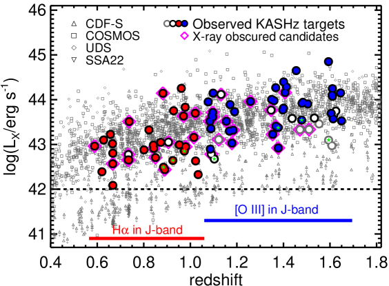
Figure 1: Hard-band (2–10 keV) X-ray luminosity versus redshift for the sources in the four deep fields covered by KASH$z$ (see Section 2.1). The dashed line indicates our luminosity cut for target selection of $L_{{\rm 2-10keV}}>10^{42}$ erg s^-1. The large symbols indicate the 89 X-ray AGN that have been observed for KASH$z$ so far. These filled and empty symbols indicate emission-line detections (H$\alpha$ or [O iii]) and no emission-line detections, respectively. Grey circles represent the 7 targets that are excluded from the analyses (i.e., resulting in a final sample of 82 targets) because a lack of an emission-line detection may be unphysical (Section 4.1). The stars highlight targets that have $L_{{\rm 2-10\,keV}}$ values estimated from the soft band (see Section 2.1). Overall the targets cover nearly three orders of magnitude in X-ray luminosity (i.e., $L_{{\rm X}}$$\approx$10⁴²–10⁴⁵ erg s^-1).

KASH$z$ is designed to ultimately obtain spatially-resolved emission-line kinematics of $\approx$(100–200) high-redshift ($z$$\approx$0.6–3.6) AGN. The overall aim of KASH$z$ is to provide insight into the feeding and feedback processes occurring in the host galaxies of high-redshift AGN by using IFS data to measure the ionised gas kinematics traced by the H$\alpha$, [O iii], H$\beta$, [N ii] and/or [S ii] emission lines. The key aspect of KASH$z$ is to exploit the unique capabilities of the multiple integral field units (IFUs) in the KMOS instrument to perform such measurements on larger, more uniformly selected samples of high-redshift AGN than was possible in previous studies that used single IFU instruments. This will make it possible to make conclusions on the overall high-redshift AGN population and to place previous observations, of a few sources, into the context of the parent population of AGN. Until now, this sort of approach has only been possible for low-redshift AGN (e.g., Harrison et al. 2014; Arribas et al. 2014; McElroy et al. 2015).

In this paper we present the first results of KASH$z$, which focuses on the galaxy-integrated emission-line profiles of $z$$\approx$0.6–1.7 X-ray detected AGN. In future papers we will present results on the spatially-resolved properties of the current sample, as well as expand the sample size when more data are obtained during our ongoing guaranteed-time KMOS observations.

2.1 Parent catalogues

For our target selection we make use of deep X-ray surveys performed in extragalactic fields (COSMOS; CDF-S; UDS and SSA22). These surveys provide an efficient method for AGN selection that is largely free from host-galaxy contamination (e.g., see review in Brandt & Alexander 2015). The chosen X-ray fields are those visible from the VLT with the deepest X-ray data available. These allow us to uniformly select large samples of AGN that can be efficiently observed with KMOS (see Section 2.6.1). The four deep fields are:

1. Cosmic evolution survey field (COSMOS; see Scoville et al. 2007). We obtain X-ray sources by combining the 1.8 Ms Chandra catalogue that covers 0.9 deg² (C-COSMOS; Elvis et al. 2009; Puccetti et al. 2009; Civano et al. 2012) with the wider and shallower 1.5 Ms XMM-Newton catalogue that covers 2.13 deg² (XMM-COSMOS; Cappelluti et al. 2009; Brusa et al. 2010). For sources detected in both surveys we use the entries in the C-COSMOS catalogue.

2. Chandra Deep Field South (CDF-S; see Giacconi et al. 2001). We use the X-ray sources from the 4 Ms Chandra catalogue that covers 464.5 arcmin² (Xue et al. 2011).

3. The Subaru/XMM-Newton Deep Survey (SXDS: see Furusawa et al. 2008). We use the X-ray sources from the 400 ks XMM-Newton catalogue that covers 1.14 deg² (Ueda et al. 2008). We only observe sources that are positioned inside the central 0.8 deg² that are also covered by the near-IR Ultra Deep Survey (UDS; see Lawrence et al. 2007). We use UDS as the name of this field hereafter.

4. The SSA22 $z=3.09$ protocluster field (see Steidel et al. 1998). We use the X-ray sources from the 400 ks Chandra catalogue that covers 330 arcmin² (Lehmer et al. 2009).

To define our sample we primarily make use of the hard-band fluxes ($F_{\rm 2-10keV}$) for each of the X-ray sources. We also make use of the soft-band fluxes ($F_{{\rm 0.5-2keV}}$) when there is no hard-band detection and for calculating the $F_{\rm 2-10keV}$/$F_{{\rm 0.5-2keV}}$ flux ratios to select X-ray obscured candidates (see Section 2.4). We note that throughout this work, $L_{X}$ refers to the hard-band (2–10 keV) luminosities. To be consistent across the four fields, we calculate fluxes making similar assumptions to the C-COSMOS catalogue (see Puccetti et al. 2009); i.e., we convert quoted count rates ($CR$) to fluxes, assuming a photon index of $\Gamma=1.4$ and a typical galactic absorption of $N_{{\rm H}}\approx 2\times 10^{20}$ cm^-2. For the SSA22 and CDF-S Chandra catalogues, we use $CR$ to flux conversion factors of 2.87$\times$10^-11 erg cm^-2 and 8.67$\times$10^-12 erg cm^-2 for the hard and soft bands, respectively. We note that these conversion factors also take into account the conversion between the quoted 2–8 keV energy-band values to 2–10 keV energy-band values. For the UDS XMM-Newton catalogue, we use the conversion factors applicable for $\Gamma$=1.4 tabulated by Ueda et al. (2008) and for C-COSMOS and XMM-COSMOS we use the quoted flux values in Puccetti et al. (2009) and Brusa et al. (2010), respectively. The X-ray fluxes are tabulated in Table 1.

We obtained archival redshifts for the sources in the fields as follows: (1) for C-COSMOS we use the compilation in Civano et al. (2012), using spectroscopic redshifts when available and photometric redshifts otherwise; (2) for CDF-S we only target sources with spectroscopic redshifts as compiled by Xue et al. (2011); (3) for UDS we used the October 2010 spectroscopic redshift compilation provided by the UDS consortium (Smail et al. 2008; Simpson et al. 2012; Akiyama et al. in prep.) and (4) for SSA22 we use the spectroscopic redshifts compiled by Lehmer et al. (2009). For our observed targets the redshifts used throughout this work, $z$, are those derived from our measured emission-lines (i.e., $z_{\rm L}$; Section 3.2), in preference to the archival redshifts (i.e., $z_{\rm A}$) described above. The archival redshifts and our emission-line redshifts for the targets presented here are tabulated in Table 1.

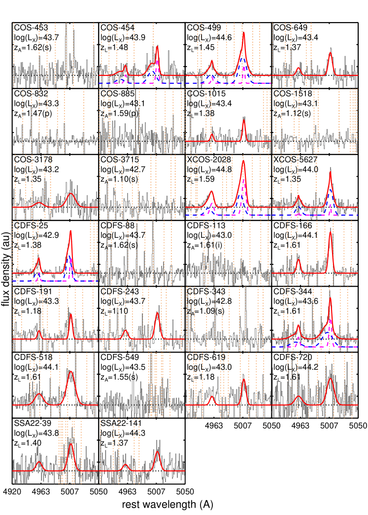
Figure 1: continued

The sources in our parent catalogues are plotted in the $L_{{\rm X}}$–redshift plane in Figure 1. We calculate X-ray luminosities following,

$$L=4\pi D_{L}^{2}F(1+z)^{\Gamma-2},$$ (1)

where $D_{L}$ is the luminosity distance, $F$ is the X-ray flux in the relevant energy band, $z$ is the redshift (see above) and $\Gamma$ is the photon index. As above, we assume $\Gamma=1.4$ for all sources. Some of the X-ray sources are detected in the soft band (0.5–2.0 keV) but not in the hard band (2–10 keV) and for these sources we make use the catalogued flux upper limits to plot them in Figure 1. However, for the targets that we observed in this work, that do not have a hard-band detection, i.e., seven targets that are all from the COSMOS field (see Table 1), we estimated hard-band fluxes by extrapolating from the soft band assuming a power-law with $\Gamma=1.4$ (see star symbols in Figure 1). In all of these cases the extrapolated hard-band fluxes were consistent with the measured upper limits and we verified that the X-ray emission was AGN-dominated (see below).

2.2 Sample selection

Our KASH$z$ targets were selected using the archival redshifts and X-ray luminosities described above. For this paper, we observed targets in the NIR $J$-band, which covers a wavelength range of $\lambda$$\approx$1.03–1.34 $\mu$m. Therefore, we selected targets with redshifts in these two ranges ranges: (1) $z$$=$1.07–1.67, for which we could observe the [O iii]4959,5007 emission-line doublet or (2) $z$$=$0.57–1.05, for which we could observe the H$\alpha$ and [N ii]6548,6583 emission lines.

To avoid selecting non-AGN X-ray sources (i.e., extreme starburst galaxies), we select sources with a measured hard-band luminosity of $L_{{\rm 2-10\,keV}}>10^{42}$ erg s^-1. We note that this X-ray luminosity has little impact on the final selection because the X-ray catalogues are not complete down to this luminosity for our redshift ranges of interest (see Figure 1). Therefore, the majority of the observed targets (i.e., all but four) have X-ray luminosities of $L_{{\rm 2-10\,keV}}>3\times 10^{42}$ erg s^-1 and will have X-ray emission that is AGN dominated; for X-ray emission of this luminosity to be produced by star-formation processes alone, it would require extreme star-formation rates of $\gtrsim$1900 $M_{\odot}$ yr^-1, based on empirical measurements of star-forming galaxies (following Equation [4] of Symeonidis et al. 2011 and Kennicutt 1998 converted to a Chabrier IMF; also see Lehmer et al. 2010). Four of our targets, all of which are in CDF-S, have $L_{{\rm 2-10\,keV}}=(1$–$3)\times 10^{42}$ erg s^-1, which could conceivably be produced by high levels of star formation; however, we verified that the X-ray emission is AGN-dominated in these sources by finding that their star-formation rates, taken from Stanley et al. (2015), are too low by a factor of $>$30 to produce the observed hard-band X-ray luminosities (following the same procedure as above). We note that Xue et al. (2011) also classify all of our CDF-S X-ray targets as AGN, using a more comprehensive X-ray and multi-wavelength identification procedure.

The initial KMOS data of KASH$z$ that are presented here, were obtained during ESO periods P92–P95 (details provided in Section 2.6.1). During these observations we obtained KMOS data for 79 X-ray AGN that met our selection criteria. This programme was jointly observed with the KROSS guaranteed time observing (GTO) programme (Stott et al. 2015) and the choice of these 79 AGN targets, drawn from our parent sample, was dictated by those that could be observed inside the KMOS pointing positions chosen by the KROSS team, with a slight preference to selecting $z$$\approx$1.1–1.7 AGN for which we could observe [O iii]. In summary, the observed targets are effectively randomly selected from the luminosity and redshift plane of the parent sample (Figure 1; also see Section 2.3 for more discussion on how representative our targets are).

We supplemented our sample of 79 KMOS targets with archival observations taken with SINFONI (Spectrograph for INtegral Field Observations in the Near Infrared; Eisenhauer et al. 2003). SINFONI contains a single-object NIR IFU, similar to the individual KMOS IFUs (see Section 2.6.2). We queried the ESO archive for $J$-band SINFONI observations at the positions of the X-ray AGN in our parent catalogues. This yielded 10 targets that met our selection criteria, to add to the $J$-band sample presented in this paper.

Overall, our current KASH$z$ sample contains 89 targets. This sample consists of 54 $z$$\approx$1.1–1.7 AGN, for which we targeted the [O iii]4959,5007 emission-line doublet and 35 $z$$\approx$0.6–1.1 AGN, for which we targeted the H$\alpha$ and [N ii]6548,6583 emission lines (see Figure 1). The targets are listed in Table 1 and we have used a naming convention that combines their field names and corresponding X-ray ID in the format: “field”-“X-ray ID”. For C-COSMOS and XMM-COSMOS the field names are shortened to COS and XCOS, respectively.

Out of the 89 targets presented here, 83 have a spectroscopic archival redshift and 6 targets have a photometric redshift. All of the photometric redshift targets are from the C-COSMOS field (Table 1). We note that two of the spectroscopic targets are classified as having “insecure” redshifts (e.g., based on low signal-to-noise ratios or single-lines; see Table 1) by Xue et al. (2011). For our emission-line detected targets (see Section 4.1), our emission-line redshifts agree with the archival redshifts, such that $|z_{L}-z_{A}|/(1+z_{L})\lesssim 0.005$, except for the following three exceptions: COS-44 ($z_{A}=1.51$; $z_{L}=0.80$) and COS-1199 ($z_{A}=0.77$; $z_{L}=0.85$), both of which had photometric archival redshifts, and CDFS-561 ($z_{A}$$=$0.80; $z_{L}$$=$0.98) which is a spectroscopic archival redshift quoted by Popesso et al. (2009). We discuss the detection rates of our targets, and how they relate to the archival redshifts, in Section 4.1. For the emission-line detected AGN, throughout this work, we define the redshift as $z=z_{L}$ and for the undetected targets or non-targeted AGN in the parent sample we use $z=z_{A}$.

2.3 The KASH$z$ sample in context

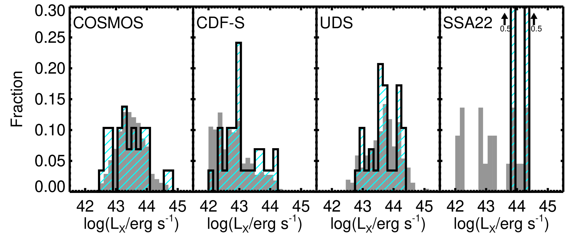
Figure 2: The 2–10 keV X-ray luminosity ($L_{{\rm X}}$) distributions for the sources that met our selection criteria from the four deep fields described in Section 2.1 (solid histograms). Each field is shown in separate panels and we overlay, as hashed histograms, the targets presented in this work that were selected from these respective fields. With the exception of SSA22 (from which there are only two targets presented here), the targets have a range of X-ray luminosities that are representative of the parent catalogues from which they were selected (see Section 2.3).

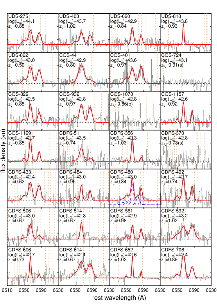
Figure 2: Galaxy-integrated spectra, shifted to the rest frame, around the H$\alpha$ and [N ii]6548,6583 emission-lines, in arbitary flux density units, for the $z\approx$ 0.6–1.1 targets that do not show a BLR component (i.e., only the Type 2 sources). For descriptions of the different curves see Figure 4. The vertical dotted lines indicate the wavelengths of the brightest sky lines (Rousselot et al. 2000). In each panel we identify the target name, the logarithm of the X-ray luminosity (in units of erg s^-1) and the redshift (see Table 1).

In Figure 2 we show histograms of the X-ray luminosities for the X-ray sources that met our selection criteria and of the subset of these that were observed for this work (Table 1). This figure shows that our targets represent the full luminosity range of the parent catalogues from which they were selected. A two-sided Kolmogorov-Smirnov (KS) test, yields probability values of 0.53, 0.08 and 0.96 that the two distributions are drawn from the same distribution for COSMOS, CDF-S and UDS, respectively. Hence, there is no evidence that the targets are not representative of the parent population from which they were selected. For SSA22 there are only two targets and hence it is not meaningful to perform a KS test. We conclude that our targets are broadly representative of the X-ray AGN population covered by the parent catalogues. It is worth noting that, although X-rays surveys arguably provide the most uniform method for selecting AGN, there will be some unknown fraction of luminous AGN that are detected at other wavelengths, that are very heavily obscured in X-rays and are not detected in these surveys (e.g., Vignali et al. 2006; Del Moro et al. 2015). We defer a comparison to AGN selected using different observational methods to future work.

2.4 Selecting X-ray obscured candidates

For part of this work we compare the emission-line properties of the targets that are most likely to be X-ray obscured (i.e., $N_{H}\gtrsim 10^{22}$ cm^-2) with those that are X-ray unobscured. Due to the use of both XMM-Newton and Chandra catalogues in our AGN selection and due to the various depths of these catalogues, we opt to use the simplest diagnostic possible to separate X-ray obscured and unobscured sources. We take the ratio of the hard-band to soft-band X-ray fluxes (i.e., $F_{{\rm 2-10keV}}/F_{{\rm 0.5-2keV}}$; see Table 1) as a proxy for an observed power-law index, $\Gamma_{{\rm obs}}$. For the seven targets where there are no direct hard-band detections, we use the hard-band flux upper limits from the original X-ray catalogues (see Section 2.1). We use a threshold of $\Gamma_{{\rm obs}}<1.4$, or equivalently $F_{{\rm 2-10keV}}/F_{{\rm 0.5-2keV}}>3.03$, to select our “obscured candidates”. Assuming a typical intrinsic power-law index of $\Gamma=1.8$ (e.g., Nandra & Pounds 1994; George et al. 2000), this threshold corresponds to an intrinsic column density of $N_{H}\gtrsim 1\times$10²² cm^-2, at the median redshift of our H$\alpha$ targets (i.e., $z=0.86$), and $N_{H}\gtrsim 2\times$10²² cm^-2, at the median redshift of our [O iii] targets (i.e., $z=1.4$). This criteria yields 32 “obscured candidates” and 52 “unobscured candidates” out of the original sample of 89. The other 5 targets have X-ray upper limit values such that they can not be classified. We identify the classification of each target in Table 1. Reassuringly, we find that only one of the obscured candidates has an identified broad-line region component in our data (see Section 3.2), compared to 15 of the unobscured candidates, as expected if X-ray obscured AGN are more likely to also have an obscured broad line region. Furthermore, this one exception only just meets our criteria for selecting obscured sources, i.e., it has a flux ratio of $F_{{\rm 2-10keV}}/F_{{\rm 0.5-2keV}}=3.1$. This provides extra support that our obscured AGN criterion is reliable.

2.5 Selecting “radio luminous” AGN

For part of this work we compare KASH$z$ targets that are radio luminous with those that are not (Section 4.3.2). Therefore, we collated the available 1.4 GHz radio catalogues for the COSMOS, CDF-S and UDS fields (a suitable SSA22 catalogue is not available in the literature). For COSMOS we used the 5$\sigma$ VLA catalogue of Schinnerer et al. (2010); for CDF-S we use the 5$\sigma$ VLA catalogue presented in Miller et al. (2013) and for UDS we use the 4$\sigma$ VLA catalogue in Arumugam et al. (2015). We match the positions of our targets to the radio positions using a 2 arcsec matching radius. For the 87 targets in these three fields (i.e., excluding the two SSA22 targets), we obtain 26 radio matches. We calculate radio luminosities using the aperture-integrated flux densities and assume a spectral index of $\alpha=-0.7$. All three catalogues have typical sensitivities around $\approx$10 $\mu$Jy beam^-1 and therefore, we are complete to 1.4 GHz radio luminosities of $L_{{\rm 1.4GHz}}\approx 10^{24}$ W Hz^-1 at the redshift ranges of interest in this work (see Figure 1). Therefore, for this work we separate our targets which are “radio luminous”, i.e., with $L_{{\rm 1.4GHz}}>10^{24}$ W Hz^-1 (11 targets) from those with $L_{{\rm 1.4GHz}}<10^{24}$ W Hz^-1 (76 targets). Table 1 highlights which targets fall into each category. Above this luminosity threshold, sources are generally thought have AGN-dominated radio emission and could be predominantly “radio-loud” sources (e.g., Del Moro et al. 2013; Bonzini et al. 2013; Rawlings et al. 2015). Furthermore, we find that 13% of our targets are in our “radio luminous” category, which is broadly consistent with the observed radio-loud fraction of $\approx$10% for luminous AGN (e.g., Zakamska et al. 2004; La Franca et al. 2010; Kalfountzou et al. 2014).

2.6 Observations

2.6.1 KMOS observations and data reduction

The majority of the KASH$z$ targets presented here (i.e., 79 out of the 89) were observed using the KMOS instrument on the VLT (Sharples et al. 2004, 2013). KMOS has 24 IFUs that operate simultaneously and can be independently positioned inside a 7.2 arcmin diameter circular field. Each IFU has a field of view of 2.8${}^{\prime\prime}\times$2.8^′′ with a pixel scale of 0.2^′′. The 24 IFUs are fed to three spectrographs (eight IFUs per spectrograph). For this initial KASH$z$ paper we present results of sources observed with the $YJ$ grating that covers a wavelength range of 1.03–1.34$\mu$m and has a band-centre spectral resolution of R$\sim$3600. The KMOS observations were taken during ESO Periods 92–95, sharing IFUs with the KROSS GTO programme, which targeted high-redshift star-forming galaxies in the same fields (see Stott et al. 2015; also see Section 3.4).

Observations were carried out using ABAABAAB sequences (where A frames are on-source and B frames are on-sky), with 600 second integrations per position and up to 0.2 arcsec spatial dithering between on-source frames. The targets have total on-source exposure times of 5.4–11.4 ks (i.e., 9–19 on-source exposures). The individual exposure times were a result of the length of observing time with acceptable weather conditions during the various observing runs allocated to the GTO team and the final on-source exposure times are tabulated for individual targets in Table 1. The median $J$-band seeing was 0.7^′′ with 90 per cent below 1.0^′′. The data were reduced using the esorex/spark pipeline (Davies et al. 2013) which flatfields, illumination corrects, wavelength calibrates and uses observations of standard stars, taken alongside the science frames, to flux calibrate. Additional sky subtraction was performed using dedicated sky IFUs. Repeated observations of targets were stacked into the final fully reduced datacubes with a clipped mean using the esorex pipeline. Finally, we rebinned the cubes onto a 0.1 arcsec pixel scale. For full details of the observations and data reduction see Stott et al. (2015).

2.6.2 SINFONI observations and data reduction

In addition to the primary observations using KMOS, we supplement the KASH$z$ sample with archival observations of 10 targets, that met our selection criteria, taken with SINFONI (see Section 2.1). The observations presented here were all observed using SINFONI’s 8$\times$8 arcsec² field of view, which is divided into 32 slices of width 0.25 arcsec with a pixel scale of 0.125 arcsec along the slices. The observations were carried out using the $J$-band grating which has an approximate resolution of $R$$\sim$3000. The observations used a variety of observing strategies, but in all cases we were able to subtract on-sky frames from on-target frames. We reduced the SINFONI data using the standard esorex pipeline (Modigliani et al. 2007) that performs flat fielding, wavelength calibration and cube re-construction. We flux calibrated individual data cubes using standard star observations taken the same night as the science observations at a similar airmass. We stacked individual cubes of the same source by creating white-light (collapsed images), centroiding the cubes based on these images and then performing a median stack with a 3$\sigma$ clipping threshold, rejecting cubes that could not be well centred. Three of the targets (CDFS-51; CDFS-370 and CDFS-492) were not detected in any of the individual cubes and for these targets, we used the offset pattern in the headers to stack the cubes. The total on-source exposure times range from 2.4–25.2 ks and are tabulated for the individual targets in Table 1.

3 Analysis and comparison samples

In this section we describe our analyses of the galaxy-integrated spectra for the targets presented in this work (Section 3.1–3.3) and we also describe our comparison samples of low-redshift AGN and high-redshift star-forming galaxies (Section 3.4).

3.1 Galaxy-integrated spectra

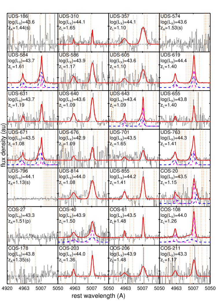
Figure 15: Galaxy-integrated spectra, shifted to the rest frame, around the [O iii]4959,5007 emission-line doublet, in arbitary flux density units, for the $z\approx$ 1.1–1.7 targets. For descriptions of the different curves see Figure 3. The vertical dotted lines indicate the wavelengths of the brightest sky lines (Rousselot et al. 2000). In each panel we also identify the target name, the logarithm of the hard-band X-ray luminosities (erg s^-1) and the redshifts (Table 1).

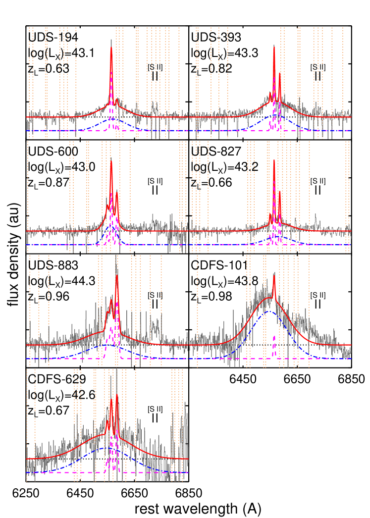
Figure 3: Same as Figure 2 but for the targets with a H$\alpha$ BLR component (i.e., the Type 1 sources). In each panel, the small thick lines show the wavelengths of the [S ii]6716,6731 emission-line doublet.

We extracted a galaxy-integrated spectrum from the KMOS and SINFONI data cubes using the methods described below. We show example spectra in Figure 3 and Figure 4 and all 89 spectra are shown in Figure 15–Figure 3.

To obtain the galaxy-integrated spectra, we initially define a galaxy “centroid” by creating wavelength-collapsed images from the data cubes, including both continuum and line-emission. For three targets no emission lines or continuum were detected and we therefore assumed the centroid was at the centre of the cube for these targets (we later exclude these three targets from our analyses; see Section 4.1). For the targets CDFS-454 and CDFS-606 there are bright continuum sources in the field of view that are spatially offset from the line-emitting regions by $\approx$2 arcsec and $\approx$1.2 arcsec, respectively. For these two targets we centred on the line emission. For each galaxy we summed the spectra from all of the pixels within a circular aperture around the galaxy centroids. We chose diameters to broadly match the physical size scale of the spectra obtained with the SDSS fibres in our low-redshift comparison sample (see Section 3.4). The median redshift of the low-redshift SDSS comparison sample is $z$=0.14 which means that the spectra are from a median 7.4 kpc diameter aperture due to the 3 arcsec fibres. For our KASH$z$ targets, the median redshift of the [O iii] sample is $z$=1.4 (i.e., corresponding to 8.4 kpc arcsec^-1) and the median redshift of the H$\alpha$ sample is $z$=0.86 (i.e., corresponding to 7.7 kpc arcsec^-1). Therefore, for the [O iii] targets we used a diameter of 0.9 arcsec and for the H$\alpha$ targets we used a diameter of 1.0 arcsec. These correspond to physical diameters of 7.6$\pm$0.8 kpc and 7.7$\pm$0.8 kpc, respectively, where the uncertainties correspond to a 0.1 arcsec pixel scale. To assess the effect of using alternative “galaxy wide” apertures, which will cover any losses of flux due to seeing, we also extracted spectra using 2^′′ diameter apertures for all sources. We discuss the corrections required to the emission-line luminosities in Section 4.2. For the sources significantly detected in both apertures, we find that our emission-line width measurements (Section 3.3) are consistent between both apertures within 1$\times$ the errors for 77% of the targets and within 2$\times$ the errors for 97% of the targets. We defer discussion of how the emission-line widths change as a function of radius to future papers.

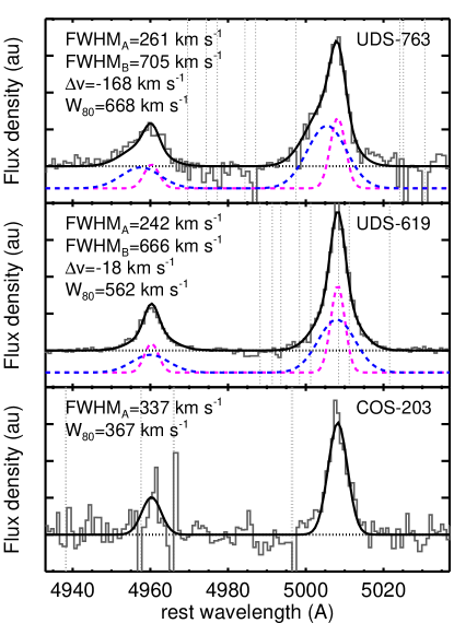
Figure 3: Three examples of our continuum-subtracted, high signal-to-noise ratio, [O iii]4959,5007 emission-line profiles. The black curves show our fits to the emission-line profiles and the dashed curves show the individual Gaussian components, where applicable, with an arbitrary offset in the y-axis. The vertical dotted lines indicate the wavelengths of the brightest sky lines (Rousselot et al. 2000). These examples demonstrate the diversity of emission-line profiles observed in the sample. Top: a broad, highly asymmetric profile; Middle: a broad, almost symmetric profile and Bottom: a relatively narrow profile without a strong underlying broad component. Figure 15 presents the [O iii]4959,5007 emission-line profiles for all of the targets.

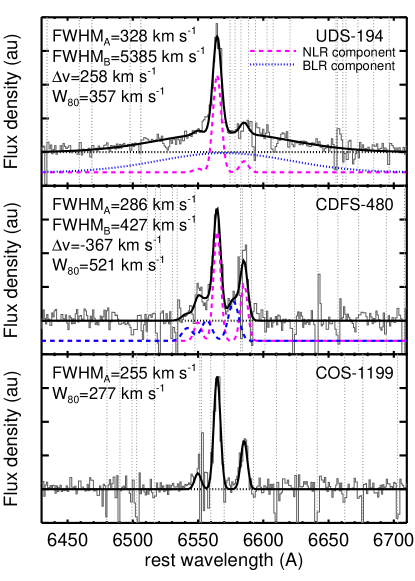
Figure 4: Three examples of our continuum-subtracted H$\alpha$+[N ii]6548,6583 emission-line profiles. The black curves show our fits to the emission-line profiles and the dashed or dot-dashed curves show the individual Gaussian components, where applicable, with an arbitrary offset. The vertical dotted lines indicate the wavelengths of the brightest sky lines (Rousselot et al. 2000). These examples represent the three different types of profile fits used in this work. Top: a source with a BLR component in addition to the NLR component; Middle: a source with no BLR component but two NLR components seen in H$\alpha$ and [N ii] and Bottom: a source with a single NLR component. Figure 2 and Figure 3 present the H$\alpha$+[N ii]6548,6583 emission-line profiles for all of the targets.

3.2 Emission-line fitting

The emission-line profiles were fit with one or two Gaussian components (with free centroids, line-widths and fluxes) and a straight line to define the local continuum (with a free slope and normalisation). The continuum regions were defined to be small wavelength regions each side of the emission lines being fitted. The noise in the spectra were also calculated in these regions. The fits were performed using a minimising-$\chi^{2}$ method, using the IDL routine MPFIT (Markwardt 2009) and we weighted against the wavelengths of the brightest sky lines (taken from Rousselot et al. 2000; see dotted lines in Figure 3 and Figure 4). Quoted line widths have been corrected for spectral resolution, where we measured the wavelength-dependant spectral resolution using the emissions lines in sky spectra. We provide details of how we modelled the emission-line profiles below and tabulate the parameters of the fits in Table 1.

For the [O iii]5007,4959 emission line doublet (see examples in Figure 15), we simultaneously fit the [O iii]5007 and [O iii]4959 emission lines using the same velocity-widths and fixing the relative centroids, using the rest-frame wavelengths of 5008.24$\AA$ and 4960.30$\AA$, respectively (i.e., their vacuum wavelengths). The flux ratio of the doublet was fixed to be 2.99 (Dimitrijević et al. 2007). We initially attempted to fit this emission-line doublet with one Gaussian component (with three free parameters) and then with two Gaussian components (with six free parameters) per emission line. We accepted the two-component fit if there is a significant improvement in the $\chi^{2}$ values. We required $\Delta\chi^{2}>15$, where this threshold was chosen to provide the best description of the emission-line profiles across the whole sample. We show the fits to the full set of [O iii]4959,5007 emission-line profiles in Figure 15.

For the H$\alpha$ emission-line profiles, along with the nearby [N ii]6548,6583 doublet, we follow a similar approach as for the [O iii] emission-line profiles (see example fits in Figure 4). Based on the atomic transition probabilities, we fix the flux ratio of the [N ii] doublet to be 3.06 (Osterbrock & Ferland 2006). To reduce the degeneracy between parameters, we couple the [N ii] and H$\alpha$ emission-line profiles with a fixed wavelength separation between the three emission lines (i.e., by using the rest-frame vacuum wavelengths of 6549.86$\AA$, 6564.61$\AA$ and 6585.27$\AA$). We also fix the line-widths of the H$\alpha$, [N ii]6548 and [N ii]6583 emission-line components to be the same. The common line-width, overall centroid and the individual fluxes of H$\alpha$ and the [N ii] doublet are free to vary. We note that the emission-line coupling is only applied for narrow-line region (NLR) components and is not applicable for broad-line region (BLR) components that are not observed in [N ii] emission. For these H$\alpha$ targets, we have two situations to consider; those which exhibit a BLR component and whose which do not.

1. For the sources where a broad component is seen in the H$\alpha$ emission-line profile but not in the [N ii] emission-line profile, these are the BLR or “Type 1” sources. We note that all seven BLR components that we identify have a full-width at half maximum (FWHM) $>$2000 km s^-1 (see Table 1), further indicating these are true BLRs. For these, we fit one Gaussian component to the [N ii]6548,6583 emission-line doublet and two Gaussian components to the H$\alpha$ emission line. The narrower of the H$\alpha$ components is coupled to the [N ii] emission as described above. The broader of these components; i.e., the BLR component, has a centroid, line-width and a flux that are free to vary. Overall, for these sources, there are seven free parameters in the fits and an example is given in the top panel of Figure 4.

2. For sources without a BLR component (i.e., the “Type 2” sources) we first fit a single Gaussian component to the H$\alpha$ emission line and [N ii] doublet, which are coupled as described above. We then add a second Gaussian component to all three emission lines. This is coupled in the same way, but with the additional constraint that we force the [N ii]/H$\alpha$ flux ratio of the broader Gaussian components to be $\gtrsim$2$\times$ that of the narrower component. This follows Genzel et al. (2014), who found that this was typical for high-redshift galaxies and AGN. This extra constraint is required to prevent considerable degeneracy in the fits that can lead to unphysical results. As for the [O iii] emission-line profiles, we accept the two component Gaussian fit if there is a significant improvement in the $\chi^{2}$ values, i.e., $\Delta\chi^{2}>15$. Examples of a one and two Gaussian component fit are shown in Figure 4.

The coupling between the [N ii] and H$\alpha$ emission-line profiles is a requirement of the restricted signal-to-noise of the observations, to avoid a high-level of degeneracy, and is not necessarily physical. The same coupling approach is often followed for high-redshift galaxies and AGN, that are inevitably subject to limited signal-to-noise observations (e.g., Swinbank et al. 2004; Genzel et al. 2011, 2014; Stott et al. 2015), and makes the underlying assumption that the emission lines are being produced by the same gas, undergoing the same kinematics (see discussion on this in Section 4.3.3). However, our emission-line profile models appear to be a good description of the data and are sufficient for our purposes of measuring the H$\alpha$ emission-line widths and luminosities and the [N ii]/H$\alpha$ flux ratios. We show the full set of fits to the H$\alpha$ emission-line profiles in Figure 2 and Figure 3 and tabulate the parameters in Table 1.

To calculate the uncertainties on the derived parameters, we follow the same procedure for both the [O iii] and H$\alpha$$+$[N ii] emission-line profiles. We use our best-fit models to generate 1000 random spectra by adding random noise to these fits, at the level measured in the original spectra, and then re-fit and re-derive the parameters for these random spectra. The quoted uncertainties are from the average of the 16th and 84th percentiles in the distribution of the parameters of these random fits. We add an additional uncertainty of 30% when plotting emission-line luminosities, to account for an estimated systematic uncertainty on the absolute flux-calibration of the data cubes.

3.3 Measuring the overall emission-line velocity widths

A key aspect of this work is to characterise the overall velocity widths of the emission-line profiles. Our spectra have a range in emission-line profile shapes and signal-to-noise values (see Figure 15–Figure 3). Therefore, it is most applicable to characterise the velocity widths with a single non-parametric measurement that is independent of the number of Gaussian components used in the best-fit emission-line models (see Section 3.2). Furthermore, many studies at low redshift use non-parametric definitions to describe the very complex emission-line profiles (e.g., Liu et al. 2013; Harrison et al. 2014; McElroy et al. 2015) and it is useful to be able to compare to these studies. Therefore, we use the line-width definition, $W_{80}$, which is the velocity width that contains 80 per cent of the emission-line flux; i.e., $W_{80}=v_{90}-v_{10}$, where $v_{10}$ and $v_{90}$ are the 10th and 90th percentiles, respectively. For a single Gaussian component $W_{80}=1.09\times$FWHM. These $W_{80}$ values are measured from the models of the emission-line profiles described in Section 3.2 and are tabulated in Table 1. For this work, we are only interested in the kinematics of the host-galaxy gas and therefore, for the 7 targets with a BLR component, the $W_{80}$ measurements only refer to the NLR emission (i.e., only the NLR components were used to calculate $W_{80}$).

3.4 Comparison samples

A key aspect of this work is to compare our high-redshift AGN targets to high-redshift star-forming galaxies and low-redshift AGN. This enables us to assess the evolution in the prevalence of outflows observed in AGN and also to compare high-redshift galaxies that do and do not host X-ray detected AGN. In the following sub-sections we describe how we constructed our comparison samples.

3.4.1 Low-redshift AGN comparison sample

For a low-redshift AGN comparison sample we make use of the catalogue provided by Mullaney et al. (2013). This sample contains emission-line profile fits to $\approx$24,000 $z<0.4$ optically-selected AGN from the SDSS spectroscopic database. AGN are identified based on their [O iii]/H$\beta$ and H$\alpha$/[N ii] emission-line ratios (following e.g., Kewley et al. 2006) or the identification of a BLR component. We take the 24,258 AGN in the Mullaney et al. (2013) catalogue, but reject the 37 sources where the [O iii] emission-line profile fits have FWHM$=$4000 km s^-1, which signifies that the fits failed for these sources (Mullaney et al. 2013). This leads to a final sample of 24,221 $z<0.4$ optically selected AGN.

Mullaney et al. (2013) fit the [O iii] emission-line profiles of the low-redshift AGN with one or two Gaussian components, following a very similar procedure to that adopted here (Section 3.2). Following Section 3.3, we measure $W_{80}$ for these sources from the [O iii] emission-line profile fits, correcting for the wavelength-dependent SDSS spectral resolution. Due to the nature of the fitting routine in Mullaney et al. (2013), the H$\alpha$ emission-line profile fits are coupled to the [O iii] emission-line profile fits. We are unable to replicate this method for our KASH$z$ H$\alpha$ targets because we do not have simultaneous [O iii] and H$\alpha$ constraints. Therefore, to avoid a biased comparison of line-width measurements, we do not use the H$\alpha$ emission-line fits provided by Mullaney et al. (2013). Instead, we use the single Gaussian component emission-line fits, as measured by the SDSS team for these targets (Abazajian et al. 2009), to calculate the $W_{80}$ values (see Section 3.3). These SDSS measurements do not separate NLR emission from BLR emission; therefore, we are required to exclude the Type 1 AGN from this comparison sample when comparing the H$\alpha$ emission-line widths to the KASH$z$ targets (Section 4.3.3). However, we note that the comparison is reasonable for our Type 2 KASH$z$ H$\alpha$ targets because all but one of the KASH$z$ Type 2 AGN are fit with a single Gaussian component.

To obtain X-ray luminosities for the $z<0.4$ AGN sample described above, we match the Mullaney et al. (2013) sample to data release 5 of the XMM serendipitous survey (Rosen et al. 2015), using a 1.5 arcsec matching radius. This resulted in 554 matches. We calculate X-ray luminosities using the quoted 2–12 keV fluxes, which we convert to 2–10 keV fluxes using a correction factor of 0.872 and convert to hard-band X-ray luminosities using Equation 1.

For part of the analysis in this work (see Section 4.3.1 and Section 4.3.3) we are required to construct low-redshift comparison samples that are luminosity-matched to our KASH$z$ samples. To do this, we randomly select sources from the sample described above to construct the following three comparison samples: (1) a low-redshift sample of $\approx$1000 AGN (both Type 1 and Type 2) that has an [O iii] luminosity distribution that is the same as our [O iii]-detected KASH$z$ targets (see Section 4.1); (2) a low-redshift sample of $\approx$100 AGN (both Type 1 and Type 2) that has an X-ray luminosity distribution that is the same as our [O iii]-detected KASH$z$ targets and (3) a low-redshift sample of $\approx$500 Type 2 AGN that has a H$\alpha$ luminosity distribution that is the same as our H$\alpha$-detected KASH$z$ targets (see Section 4.1). It was not possible to construct an low-redshift sample that was X-ray luminosity matched to our KASH$z$ H$\alpha$ targets, due to the lack of X-ray luminous Type 2 AGN in Mullaney et al. (2013). However, we note that matching by [O iii] luminosity compared to matching by X-ray luminosity does not change the conclusions presented in Section 4.3.1.

3.4.2 High-redshift star-forming galaxy comparison sample

To construct a high-redshift galaxy comparison sample we make use of the KROSS survey (Stott et al. 2015). This is a KMOS GTO survey of $z$$\approx$0.6–1.1 star-forming galaxies, which was observed simultaneously with KASH$z$ (see Section 2.6.1). These targets were selected on the basis of their K-band magnitudes and $r$–$z$ colours, to create a sample of star-forming galaxies with stellar masses of $\approx$$10^{9-11}$ M_⊙ (see Stott et al. 2015). This data set provides an ideal comparison sample of galaxies for our H$\alpha$ sample of X-ray detected AGN, at the same redshift.

The initial phases of the KROSS survey, i.e., the data obtained during ESO periods P92–P94 and the KMOS commissioning run, contains 514 galaxies (Stott et al. 2015). For these KROSS galaxies, we extract galaxy-integrated spectra from the KMOS data cubes and perform emission-line profile fits following the same methods as performed on the KASH$z$ sample (see Section 3.2 and Section 3.3). We require that H$\alpha$ emission is detected at $\geq$3$\sigma$ and the emission-line profiles are well described using one or two Gaussian components plus a straight-line local continuum (i.e., following our methods described in Section 3.2). Based on these criteria, we end up with $W_{80}$ H$\alpha$ measurements for 378 of the KROSS galaxies, where we have also removed any X-ray AGN. In our analyses (Section 4.3.3), we also make use of the stellar masses for these galaxies, as described in Stott et al. (2015) and note that the average stellar mass of the sample we have constructed is $\log(M_{\star}/M_{\odot})$=10.3.

3.5 Emission-line profile stacks

As part of our investigation we create average emission-line profiles by using spectral stacking analyses on the KASH$z$ targets and comparison samples (see Section 4.3.1 and Section 4.3.3). To create the emission-line profile stacks, we de-redshift each continuum-subtracted spectrum to the rest frame and then normalise each spectrum to the peak flux density of the emission-line profile fits. We then construct the stacked average spectra by taking a mean of the flux densities at each spectral pixel, but removing the pixels affected by strong sky-line residuals. An uncertainty on the average at each spectral pixel is obtained by bootstrap resampling, with replacement, the stacks 1000 times and deriving the inner 68 per cent of these stacks. Our analysis is focused on the kinematics in the host galaxies and therefore, when stacking the H$\alpha$ emission-line profiles, we do not include any Type 1 sources (i.e., those containing an identified BLR component). We fit the stacked spectra following the procedures described in Section 3.2; however, due to the increased signal to noise we include one extra free parameter when fitting the H$\alpha$ emission-line profiles which allows the flux ratio of the H$\alpha$ and [N ii] emission lines to be free for both Gaussian components. This means that is is possible for the [N ii] and H$\alpha$ emission lines to have different line widths (i.e., $W_{80}$ values; see discussion in Section 4.3.3).

4 Results and discussion

We present the first results from KASH$z$, which is an ongoing programme that is utilising VLT/KMOS GTO to build up a large sample of IFS data of high-redshift AGN (see Section 2). We have obtained new KMOS observations and combined them with archival SINFONI observations, to compile a sample of 89 X-ray detected AGN observed in the $J$-band. These AGN have redshifts of $z$=0.6–1.7 and hard-band (2–10 keV) X-ray luminosities in the range of $L_{{\rm X}}=10^{42}$–10⁴⁵ erg s^-1 and are representative of the parent population from which they were selected (see Figure 1 and Figure 2). Of the 89 targets presented here, 54 have $z$=1.1–1.7 and were targeted to observe the [O iii]4959,5007 emission-line doublet and 35 have $z$=0.6–1.1 and were targeted to observe the H$\alpha$+[N ii]6548,6583 emission lines. In this paper, we present the galaxy-integrated emission-line profiles for all 89 targets and these are shown, along with their emission-line profile fits, in Figure 15–Figure 3. In the following sub-sections we present: (1) the emission-line detection rates and definition of the final sample of 82 targets used for all further analyses (Section 4.1); (2) the relationship between emission-line luminosities and X-ray luminosities (Section 4.2); and (3) the prevalence and drivers of high-velocity ionised outflows (Section 4.3).

4.1 Detection rates and defining the final sample

We detected continuum and/or emission lines in the IFS data for 86 out of the 89 KASH$z$ targets (i.e., 97 per cent) (see Table 1 for details). Overall, 40 targets were detected in [O iii], 32 were detected in H$\alpha$ and 14 were detected in continuum only. One of the reasons for a lack of an emission-line detection appears to be due to inaccurate photometric redshifts (photometric redshifts were only used for six COSMOS targets; see Section 2.2). Of the six targets with photometric archival redshifts, only two resulted in emission-line detections and one of these was detected in H$\alpha$ with $z_{{\rm L}}\approx 1.5$, despite an archival redshift of $z_{{\rm A}}\approx 0.8$ (see Table 1). To ensure that a target is undetected in line emission because of an intrinsically low emission-line flux, as opposed to an incorrect redshift or position, for all further analyses we only consider non-detections if: (1) they have a secure spectroscopic archival redshift (this excludes 5 non-detections) and (2) they were detected in continuum so that we have a reliable source position to extract the spectrum from the datacube (this excludes 2 further non-detections). Based on these exclusions, for the remainder of this work, we only consider 82 of the original 89 targets, which consists of: (a) 40 emission-line detected [O iii] targets and 8 [O iii] targets that were only detected in continuum (i.e., a 83 per cent emission-line detection rate) and (b) 32 emission-line detected H$\alpha$ targets and 2 H$\alpha$ targets that were detected only in continuum (i.e., a 94 per cent emission-line detection rate). Overall this results in an emission-line detection rate of 88 per cent for our final sample of 82 targets.

We note here that the non emission-line detected sources are not only associated with the lowest X-ray luminosity sources (see Figure 5 and Figure 6). However, of the 10 targets from our final sample of 82, that were not detected in emission lines, 5 of them are classified as X-ray obscured, 4 are classified as unobscured and 1 is unclassified, which results in a 50–60% obscured fraction, compared to 33–38% for the 72 emission-line detected targets (see Section 2.4 and Table 1). Although we can not draw any firm conclusions from this, it is interesting to speculate that this provides evidence that the material obscuring the X-rays may also be responsible for the lack of emission-line luminosity and therefore that the obscuring material may be associated with the host galaxy (i.e., galactic-scale dust; see e.g., Malkan et al. 1998; Goulding & Alexander 2009; Juneau et al. 2013).

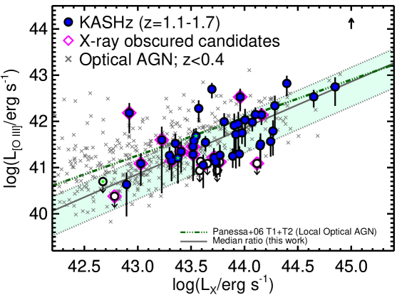
Figure 5: Total [O iii] emission-line luminosity ($L_{{\rm[O~{}III]}}$) versus hard-band (2–10 keV) X-ray luminosity ($L_{{\rm X}}$) for the 48 $z\approx 1.1$–1.7 KASH$z$ targets. Non-detections are represented as hollow symbols, which signify 3$\sigma$ upper limits, and stars are the same as in Figure 1. The solid line shows the median ratio of $\log(L_{{\rm[O~{}III]}}/L_{{\rm X}})=-2.1_{-0.5}^{+0.3}$ for these 48 KASH$z$ [O iii] targets. The shaded region indicates the $\approx$1$\sigma$ scatter on this ratio (see Section 4.2). The arrow shows the median aperture correction when using a $\approx$2$\times$ larger aperture (see Section 4.2). The dot-dashed line is the relationship for local Seyferts and QSOs presented in Panessa et al. (2006). We also show our $z<0.4$ optical AGN comparison sample (see Section 3.4). The X-ray selected KASH$z$ sample is broadly consistent with the low-redshift optically selected samples, but with the expected tendency towards lower [O iii] luminosities (Section 4.2).

4.2 Emission-line luminosities compared to X-ray luminosities

4.2.1 [O iii] luminosity versus X-ray luminosity

Both the [O iii] emission-line luminosity and X-ray luminosity have been used to estimate total AGN power (i.e., bolometric luminosities) and therefore, the relationship between these two quantities and any possible redshift evolution, is of fundamental importance for interpreting observations (e.g., Mulchaey et al. 1994; Heckman et al. 2005; Panessa et al. 2006; Netzer et al. 2006; LaMassa et al. 2009; Lamastra et al. 2009; Trouille & Barger 2010; Lusso et al. 2012; Berney et al. 2015). Until recently, there has been limited available NIR spectroscopy and therefore limited measurements of the [O iii] emission-line luminosities for high-redshift, i.e., $z\gtrsim 1$, X-ray detected AGN. In this sub-section we compare the [O iii] and X-ray luminosities for our final KASH$z$ sample of 48 $z$$\approx$1.1–1.7 AGN that were targeted to observe [O iii] emission (see Section 4.1).

In Figure 5 we show [O iii] luminosity versus X-ray luminosity for the KASH$z$ targets. A correlation is observed between these two quantities, although with a large scatter, in qualitative agreement with studies of low-redshift AGN (e.g., Heckman et al. 2005; Panessa et al. 2006). We note that we observe the same trend when plotting [O iii] flux versus X-ray flux and therefore the correlation is not an artifact of flux limits. For the 48 targets, we find a median luminosity ratio of $\log(L_{{\rm[O~{}III]}}/L_{{\rm X}})=-2.1^{+0.3}_{-0.5}$, where the quoted upper and lower bounds contain the inner 66 per cent of the targets, i.e., roughly the 1$\sigma$ scatter. To calculate the median ratio of [O iii] to X-ray luminosity we have assumed that the non emission-line detected [O iii] targets fall into the bottom 50% of this distribution. Furthermore, to give the quoted range, we have assumed that they intrinsically fall in the bottom 17 per cent of the $L_{{\rm[O~{}III]}}/L_{{\rm X}}$ distribution. These are not unreasonable assumptions given that all but one of these targets have 3$\sigma$ upper limits that fall very close to, or below, this boundary (see Figure 5). We note that, if we make our [O iii] luminosity measurements using a 2^′′ aperture (see Section 3.1) we find a median aperture correction of 0.28 dex with a scatter of 0.09 dex. Therefore, using “total” luminosities could increase our quoted $L_{{\rm[O~{}III]}}/L_{{\rm X}}$ ratio by $\approx$0.3 dex (see Figure 5). Overall, our results indicate that, typically, [O iii] luminosities are $\approx$1% of the X-ray luminosities, with a factor of 2–3 scatter, for $z\approx$1.1–1.7 X-ray detected AGN.

To compare to low-redshift AGN, in Figure 5, we show the objects from our $z<0.4$ AGN comparison sample (see Section 3.4) and the relationship found for local Seyfert galaxies and QSOs by Panessa et al. (2006). The KASH$z$ targets appear to broadly cover the same region of the $L_{{\rm[OIII]}}-L_{{\rm X}}$ parameter space as the $z<0.4$ AGN, but with a slight tendency towards lower [O iii] luminosities. This may be partly due to the different approaches used (or not used) to aperture-correct the luminosities or a lack of correction for reddening to the [O iii] emission-line measurements. Furthermore, the $z<0.4$ AGN are initially drawn from an optically selected SDSS sample, which is [O iii] flux limited (see Section 3.4), while, in contrast, the KASH$z$ is initially X-ray selected. Indeed, a plot of [O iii] flux versus X-ray flux reveals that the deficit of low $L_{{\rm[OIII]}}/L_{{\rm X}}$ luminosity ratios in the $z<0.4$ sample, observed in Figure 5, is at least partly driven by the [O iii] flux limit. Heckman et al. (2005) and Lamastra et al. (2009) present further discussion on the difference between optically selected and X-ray selected samples.

The majority of the KASH$z$ [O iii] targets cover a narrow X-ray luminosity range (i.e., $L_{{\rm X}}$=2$\times$10⁴³–2$\times$10⁴⁴ erg s^-1; see Figure 5); therefore, we do not attempt to fit a luminosity-dependant relationship between $L_{{\rm X}}$ and $L_{{\rm[O~{}III]}}$. However, we note that the local $L_{{\rm X}}$–$L_{{\rm[O~{}III]}}$ relationship is found to be close to linear in log-log space, when measured over five orders of magnitude in X-ray luminosity (i.e., $\log L_{{\rm[O~{}III]}}\propto(0.82\pm 0.08)\log L_{{\rm X}}$; Panessa et al. 2006; also see Lamastra et al. 2009 for an even more linear relationship for a combined sample of optical and X-ray selected AGN). At the median X-ray luminosity of our [O iii] KASH$z$ sample, i.e., $\log(L_{{\rm X}}$/erg s${}^{-1})=43.7$, the local relationship from Panessa et al. (2006) results in a luminosity ratio of $\log(L_{{\rm[O~{}III]}}/L_{{\rm X}})=-1.86$, which is consistent with our KASH$z$ value of $-2.1^{+0.3}_{-0.5}$. Therefore, based on these data, we have no reason to conclude that there is any significant difference between the $L_{{\rm X}}$–$L_{{\rm[O~{}III]}}$ relationship for our $z$$\approx$1.1–1.7 sample compared to local AGN.

In Figure 5 we observe a large scatter of a factor of $\approx$3. This is similar to the scatter seen in local X-ray selected AGN by Heckman et al. (2005). The lack of a correction for X-ray obscuration may account for some of this scatter; however, we note that the obscuration correction to hard-band (2-10 keV) luminosities, at these redshifts, will be small except in the most extreme cases (e.g., Alexander et al. 2008; although see LaMassa et al. 2009). A more significant factor on the amount of scatter will be the effect of various amounts of dust reddening, in the host galaxy, that will affect the [O iii] emission-line luminosities (see e.g., Panessa et al. 2006; Netzer et al. 2006). Due to the lack of sufficient constraints on this reddening effect across the sample, we do not attempt to correct for this effect. A more interesting interpretation of the larger scatter in this diagram is a possible lack of uniformity in the amount of gas inside the AGN ionisation fields due to variations in opening angles and inclinations, with respect to the host-galaxy gas. These effects will lead to different volumes of gas being photoionised by the central AGN. One further possible interpretation for the large scatter observed in Figure 5 is the different timescales of the accretion rates being traced by X-ray versus [O iii] luminosity. Whilst the X-ray emission primarily traces nuclear activity associated with the region very close to the accretion disk (e.g., Pringle 1981), the [O iii] emission is found in NLRs, which can extend on $\approx$0.1–10 kpc scales (e.g., Boroson et al. 1985; Osterbrock & Ferland 2006; Hainline et al. 2013). Therefore, a NLR that is photoionised by an AGN could act as an isotropic tracer of the time-averaged bolometric AGN luminosity over $\approx$10⁴ years, while in contrast, the X-ray luminosity is an instantaneous measurement of the bolometric AGN luminosity (see e.g., Hickox et al. 2014; Schawinski et al. 2015; Berney et al. 2015 for further discussion on the relative timescales of different AGN tracers).

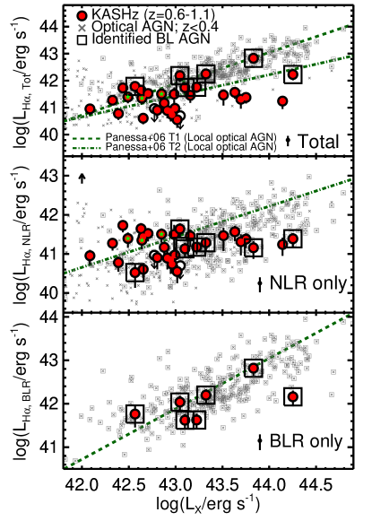
Figure 6: H$\alpha$ emission-line luminosity ($L_{{\rm H}\alpha}$) versus hard-band (2–10 keV) X-ray luminosity ($L_{{\rm X}}$) for the 34 $z$$\approx$0.6–1.1 KASH$z$ H$\alpha$ targets. In the top panel we show the total emission-line luminosities, in the middle panel we show the luminosities where the BLR components have been subtracted (i.e., the NLR luminosities) and in the bottom panel we show the BLR luminosities, where applicable. Non-detections are represented as hollow symbols, which signify 3$\sigma$ upper limits, and the stars are the same as in Figure 1. For clarity, the median uncertainty on the line luminosities is shown at the bottom of each panel. The arrow in the second panel shows the median aperture correction when using a $\approx$2$\times$ larger aperture (see Section 4.2). The dashed and dot-dashed lines show the luminosity-dependent relationships for Type 1 (T1) and Type 2 (T2) local AGN presented in Panessa et al. (2006). We also show our $z<0.4$ optical AGN comparison sample (see Section 3.4).

4.2.2 H$\alpha$ luminosity versus X-ray luminosity

The H$\alpha$ emission-line luminosity is a very common tracer of star-formation rates in local and high-redshift galaxies (e.g., see Kennicutt 1998; Calzetti 2013). However, this is complicated in AGN host-galaxies for two main reasons. Firstly, H$\alpha$ emission is also produced in the sub-parsec scale BLRs around SMBHs, which are most likely to be photoionised by the central AGN and, secondly, the gas in the kpc-scale NLR of AGN can also be photoionised by the AGN (e.g., Osterbrock & Ferland 2006). The relative contribution of AGN versus star-formation to producing the total H$\alpha$ luminosity ($L_{{\rm H\alpha}}$) will significantly affect how well correlated $L_{{\rm H\alpha}}$ is with tracers of bolometric AGN luminosity, such as the hard-band X-ray luminosity ($L_{{\rm X}}$). In this sub-section we compare the H$\alpha$ and X-ray luminosities for our final KASH$z$ sample of 34 $z$$\approx$0.6–1.1 AGN that were targeted to observe H$\alpha$ emission (see Section 4.1).

In Figure 6 we show $L_{{\rm H\alpha}}$ versus $L_{{\rm X}}$ for our KASH$z$ targets. In the middle and bottom panels we separate the H$\alpha$ luminosity into that associated with the NLRs (i.e., $L_{{\rm H\alpha,NLR}}$) and that associated with the BLRs (i.e., $L_{{\rm H\alpha,BLR}}$), respectively (see Section 3.2 for details of how we separate these components). Following from our [O iii] analyses in the previous section, we do not attempt to correct for X-ray obscuration or dust reddening (although see discussion below). In Figure 6 we also show our $z<0.4$ AGN comparison sample (see Section 3.4) and the relationships found for local AGN and QSOs by Panessa et al. (2006). We note that, if we make our H$\alpha$ NLR luminosity measurements using a 2^′′ aperture (see Section 3.1) we find a median aperture correction of 0.25 dex with a scatter of 0.08 dex.

In the bottom panel of Figure 6 it can be seen that there is a correlation between BLR region luminosity, $L_{{\rm H\alpha,BLR}}$, and $L_{{\rm X}}$ for the $z<0.4$ AGN. These sources broadly follow the local relationship observed for the Type 1 Seyferts and QSOs by Panessa et al. (2006), i.e., $\log L_{{\rm H\alpha,T1}}\propto(1.16\pm 0.07)\log L_{{\rm X}}$. Although we are limited to seven BLR sources for the KASH$z$ sample, our targets are found to be within the scatter of the $z<0.4$ AGN, and therefore they qualitatively follow the same relationship as low-redshift and local AGN (see Figure 6). It is not surprising that the BLR luminosities are tightly correlated with the X-ray luminosities (see Figure 6). The BLR is directly illuminated by the central AGN, which is also responsible for the production of X-rays around the accretion disk (e.g., Pringle 1981; Osterbrock & Ferland 2006). Furthermore, due to the size scales of the BLR that are typically on light-days to light-months (e.g., Peterson et al. 2004), the relative timescales of the accretion events being probed by the X-ray emission and BLR emission will be much closer compared to the relative timescales between the X-ray emission and the kpc-scale NLR emission (see discussion above for the [O iii] NLR emission).

In contrast to the BLR luminosities, there is little-to-no evidence for a correlation observed between the NLR H$\alpha$ luminosity and X-ray luminosity for both the KASH$z$ sample and the $z<0.4$ comparison sample (see the middle panel of Figure 6). In qualitative agreement with this for local AGN, the relationship is less steep for Type 2 AGN compared to Type 1 AGN and QSOs by Panessa et al. (2006); i.e., $\log L_{{\rm H\alpha,T2}}\propto(0.78\pm 0.09)\log L_{{\rm X}}$. However, some correlation does still exist in local samples, whereas we do not see evidence for this in our current high-redshift sample. In addition to the timescale arguments already discussed, this may be due to additional contributions to the NLR H$\alpha$ luminosities, in addition to photoionisation by AGN, such as by star-formation processes (e.g., Cresci et al. 2015). Indeed we observe that a significant fraction of our sample have [N ii]/H$\alpha$ emission-line ratios that could be produced by H ii regions (see Section 4.3.3). The NLR region H$\alpha$ luminosities of the KASH$z$ targets may follow an even shallower trend than the local relationship; however, the deviation is only observed at the highest X-ray luminosities, where we are currently limited to a lower number of sources (see Figure 6). We also note that the KASH$z$ AGN are likely to be systematically low in $L_{{\rm H\alpha,NLR}}$ due to the lack of obscuration correction (also see the discussion on aperture effects above). For example, the correction to the NLR luminosities would be $\approx$0.7 dex, assuming the median $A_{{\rm V,H\alpha}}=1.7$ for the star-forming galaxy comparison sample at the same redshift (Stott et al. 2015; Section 3.4), while the average Balmer decrement of the $z<0.4$ AGN comparison sample implies a median correction of only $\approx$0.3 dex for the $z<0.4$ AGN (following Calzetti et al. 2000). Additionally, our X-ray selection compared to the optically selected comparison samples may also provide a systematic effect towards lower line luminosities for the high-redshift sources (see discussion above for the [O iii] targets).

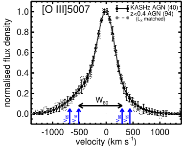
Figure 7: Stacked [O iii]5007 emission-line profiles for the 40 [O iii] detected KASH$z$ targets and the X-ray luminosity matched $z<0.4$ AGN comparison sample (see Section 3.4). The dotted curves show the stacked data and the dashed and solid curves are fits to these stacks. The upward arrows show, from left-to-right, the 5th, 10th, 90th and 95th percentile velocities of the KASH$z$ stack. The overall emission-line width of $W_{80}$=810 km s^-1 is also illustrated (see Section 3.3). On average, the KASH$z$ AGN show a broad and asymmetric emission-line profile, with velocities reaching $\approx$1000 km s^-1. The low-redshift AGN have a very similar average emission-line profile to the high-redshift AGN, for these luminosity-matched samples.

4.3 The prevalence and drivers of ionised outflows

A key aspect of KASH$z$ is to constrain the prevalence of ionised outflow features observed in the emission-line profiles of high-redshift AGN. Additionally, KASH$z$ is designed to assess which AGN and host-galaxy properties are associated with the highest prevalence of high-velocity outflows. One of the most common approaches to search for ionised outflows is to look for very broad and/or asymmetric emission-line profiles in the ionised gas species such as [O iii] and non-BLR H$\alpha$ components (e.g., Heckman et al. 1981; Veilleux 1991; Mullaney et al. 2013; Zakamska & Greene 2014; Genzel et al. 2014). For example, asymmetric emission-line profiles (most commonly a blue wing) that reach high velocities (i.e., $\approx$1000 km s^-1) are very difficult to explain other than through outflowing material (e.g.,Veilleux 1991; Zakamska & Greene 2014). Furthermore, extremely broad emission-line profiles (i.e, $W_{80}\gtrsim 600$ km s^-1) are very unlikely to be the result of galaxy kinematics, but instead trace outflows or high levels of turbulence (e.g., Vega Beltrán et al. 2001; Collet et al. 2015; also see discussion in Section 4.3.3) and studies of large samples of low-redshift AGN have shown that the gas that is producing such broad emission-line profiles is not in dynamical equilibrium with their host galaxies (see Liu et al. 2013 and Zakamska & Greene 2014).

In the following sub-sections we assess the prevalence and drivers of ionised outflow features in the galaxy-integrated emission-line profiles of our KASH$z$ AGN sample, following similar methods to Mullaney et al. (2013) who study $z<0.4$ AGN (see Section 3.4). More specifically, we investigate the distributions of emission-line velocity widths of individual sources, in combination with emission-line profile stacks. For clarity and ease of comparison to previous studies, we separate the discussion of the $z$$\approx$1.1–1.7 [O iii] sample from the $z$$\approx$0.6–1.1 H$\alpha$ sample (these are defined in Section 4.1). Furthermore, the [O iii] emitting gas is more likely to be dominated by AGN illumination, while the H$\alpha$ emission may also have a significant contribution from star formation (see discussion in Section 4.3.3). We defer a detailed comparison of these two ionised gas tracers to future papers, which will be based on spatially-resolved spectroscopy using both emission lines for the same targets; however, see the works of Cano-Díaz et al. (2012) and Cresci et al. (2015) for IFS data covering both H$\alpha$ and [O iii] measurements for two high-redshift AGN.

4.3.1 The distribution of [O iii] emission-line velocity widths

In Figure 15 we show the [O iii] emission-line profiles, and our best-fitting solutions, for all the $z$$\approx$1.1–1.7 KASH$z$ targets. The parameters of all of the fits are provided in Table 1. We identify secondary broad components (following the methods described in Section 3.2), with FWHM$\approx$400–1400 km s^-1, in the emission-line profiles for 14 out of the 40 [O iii] detected targets (i.e., 35 per cent). The velocity offsets of these broad components, with respect to the narrow components, reach up to $|\Delta v|\approx 500$ km s^-1. We note that Brusa et al. (2015) find that four out of their eight $z\approx$1.5 X-ray luminous AGN identify a secondary broad emission-line component at high-significance in their [O iii] spectra, which is broadly consistent with our fraction given the low numbers involved. While the fraction of broad emission-line components in our KASH$z$ sample already indicates a high prevalence of high-velocity ionised gas in high-redshift X-ray AGN, these measurements do not provide a complete picture across all of the targets. This is because it is very difficult to detect multiple Gaussian components when the signal-to-noise ratio is modest; i.e., the detection of a second Gaussian component is limited to the highest signal-to-noise ratio spectra. Therefore, in the following discussion, we follow two methods to overcome these challenges. Firstly we assess the average emission-line profiles using stacking analysis (see Section 3.5) and, secondly, we use a non-parametric definition to characterise the overall line width, (i.e., $W_{80}$ which is the width that encloses 80 per cent of the emission-line flux; see Section 3.3).

We show the stacked [O iii]5007 emission-line profile for our KASH$z$ targets in Figure 7. The overall-emission line width of this average profile is $W_{80}$=810${}^{+130}_{-220}$ km s^-1 (see Section 3.3), where the upper and lower bounds indicate the 68 per cent range from bootstrap resampling that stack. This indicates that, on average, the ionised gas in these AGN have high-velocity kinematics, that are not associated with the host galaxy dynamics. Furthermore, the average emission-line profile clearly shows a luminous blueshifted broad wing, which reveals high-velocity outflowing ionised gas out to velocities of $\approx$1000 km s^-1. A preference for blueshifted broad wings, compared to redshifted broad wings, has been previously been observed for both high- and low-redshift AGN samples (e.g., Heckman et al. 1981; Vrtilek 1985; Veilleux 1991; Harrison et al. 2012; Mullaney et al. 2013; Zakamska & Greene 2014; Balmaverde et al. 2015). This can be explained if the far-side of any outflowing gas, that is moving away from the line of sight, is obscured by dust in the host galaxies (e.g., Heckman et al. 1981; Vrtilek 1985). To observe a redshifted component, the outflow would need to be highly-inclined or extended beyond the obscuring material (e.g., Barth et al. 2008; Crenshaw et al. 2010; Harrison et al. 2012; Rupke & Veilleux 2013).

While informative, the average emission-line profile shown in Figure 7 hides critical information on the underlying distribution of ionised gas kinematics in our sample. Therefore, in Figure 8 we show the distribution of the [O iii] velocity-width values, $W_{80{\rm,[O~{}III]}}$, for the individually [O iii] detected targets. In the top panel we show the raw distribution and in the bottom panel we show the cumulative distribution. 1$\sigma$ uncertainties on the cumulative distribution have been calculated assuming Poisson errors, suitable for small number statistics, following the analytical expressions provided by Gehrels (1986). We use the same uncertainty calculations for all of the percentages presented for the remainder of this section. We find that 50${}^{+14}_{-11}$ per cent of the [O iii] targets have velocity-widths indicative of tracing ionised outflows or highly turbulent material, i.e., $W_{80{\rm,[O~{}III]}}>600$ km s^-1 (e.g. Liu et al. 2013; Collet et al. 2015). This fraction ranges over (42–58) per cent, when including the 8 non-detected targets (see Section 4.1), for which we have no $W_{80{\rm,[O~{}III]}}$ measurements.

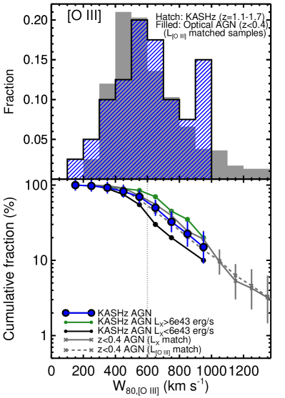
Figure 8: Top: Histograms of the overall emission-line velocity width, $W_{{\rm 80,[OIII]}}$, for the 40 $z\approx$1.1–1.7 [O iii] detected KASH$z$ targets (hatched) and a luminosity-matched sample of 1000 $z<0.4$ optical AGN (filled; see Section 3.4). The KASH$z$ AGN show a very similar distribution of velocities as the luminosity-matched low-redshift AGN sample. This is further demonstrated in the bottom panel which shows the cumulative distributions. We split the KASH$z$ sample in half, separating at $L_{X}=6\times 10^{43}$ erg s^-1, and find that high-velocity gas kinematics are more prevalent in higher luminosity AGN; for example, it is $\gtrsim$2$\times$ more likely that the higher luminosity AGN have $W_{80}\gtrsim$ 600 km s^-1, compared to the lower-luminosity AGN (see vertical dotted line; Section 4.3.2).

To compare the prevalence of outflow features in our high-redshift AGN sample, to low-redshift AGN, we show the distribution of velocity-widths for our $z<0.4$ luminosity-matched comparison samples in Figure 8 (see Section 3.4). The luminosity-matching is performed to account for the observed correlation between luminosity and emission-line widths (Mullaney et al. 2013; also see Section 4.3.2). We note that we obtain the same conclusions if we match by either $L_{{\rm[OIII]}}$ or $L_{{\rm X}}$. In Figure 8, the [O iii] line-width distributions look indistinguishable between the KASH$z$ sample and the luminosity-matched $z<0.4$ AGN samples. A two-sided KS test shows no evidence that the two different redshifts have significantly different velocity-width distributions (i.e., a $\approx$60 per cent chance that the two redshift ranges have velocity-width values drawn from the same distribution). In Figure 7, we further demonstrate that luminosity-matched AGN, from both redshift-ranges, have similar [O iii] emission-line profiles by showing that the stacked emission-line profiles look the same. This result implies that the prevalence of ionised outflows in low-redshift and high-redshift AGN are very similar for AGN of the same luminosity. This is despite the fact that the average star-formation rates of X-ray AGN are $\approx$10$\times$ higher at $z$$\approx$1 compared to $z\approx$0.2, irrespective of X-ray luminosity (Stanley et al. 2015). Therefore, this result provides indirect evidence that the prevalence of these high-velocity outflows is not greatly influenced by the level of star formation. We draw similar conclusions for the H$\alpha$ KASH$z$ sample in Section 4.3.3.

Using our representative targets (see Figure 2 and Section 2.3), it is now possible to place some previous observations of high-redshift X-ray AGN into the context of the overall population. For example, the SINFONI observations of XCOS-2028 were used by Cresci et al. (2015) to present evidence of star-formation suppression by the outflow observed in this source (see our spectra for this source in Figure 15). This conclusion was based on their observed deficit of NLR H$\alpha$ emission, a possible tracer of star formation (see Section 4.2 and Section 4.3.3), in the location of the outflowing [O iii] component. Based on our analyses, this source has an emission-line velocity width of $W_{80}\approx 730$ km s^-1. We find $\approx$30 per cent of the overall X-ray AGN population have these emission-line widths or greater. Therefore, this target does not have an exceptional outflow; however, it is yet to be determined how common the observed deficit of NLR H$\alpha$ emission in this source is in the overall high-redshift AGN population.

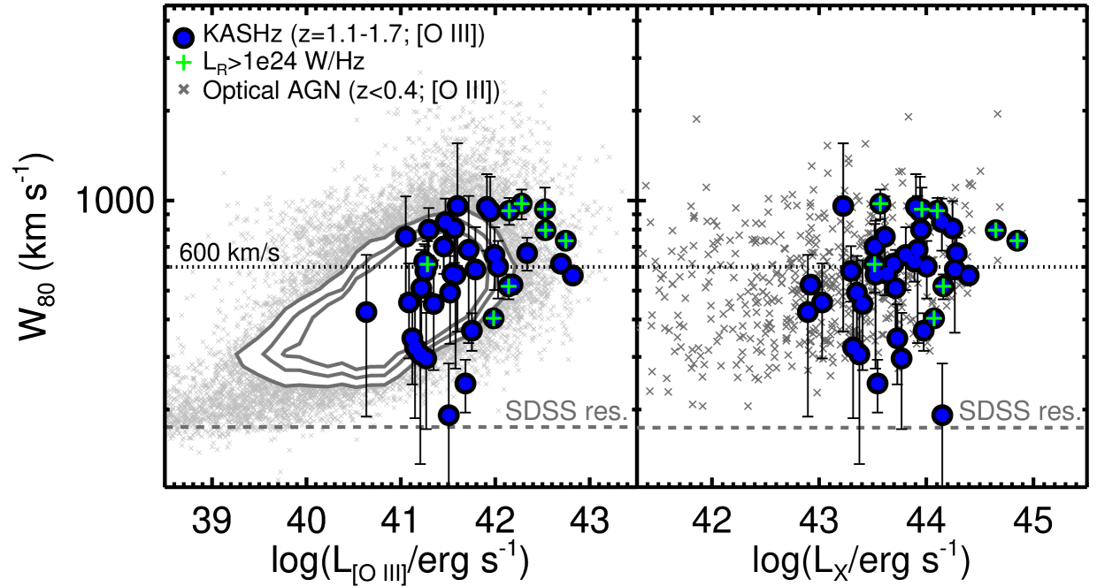
Figure 9: Emission-line velocity width ($W_{80}$) versus [O iii] luminosity (left) and hard-band (2–10 keV) X-ray luminosity (right) for the $z\approx$1.1–1.7 KASH$z$ sample (circles) and the $z<0.4$ AGN comparison sample (contours and crosses). The dashed lines show the $W_{80}$ value for the median spectral resolution for the $z<0.4$ sources. Although a wide distribution of velocities are observed, the most luminous AGN (either by line luminosity or X-ray luminosity) preferentially host extreme gas velocities. For example, all of the KASH$z$ AGN with $L_{{\rm[O~{}III]}}>10^{42.2}$ erg s^-1 have velocity-widths of $\gtrsim$600 km s^-1 (see dotted line).

4.3.2 The physical drivers of the high-velocity outflows observed in [O iii]

It is of fundamental importance to constrain how AGN and host-galaxy properties are related to the prevalence and properties of galaxy-wide outflows. For example, in most cosmological models, the accretion rates of the AGN fundamentally determine the velocities and energetics of the outflows (e.g., Schaye et al. 2015), while some models, concentrating on individual sources, have invoked the mechanical output from radio jets as a plausible outflow driving mechanism (e.g., Wagner et al. 2012). In this sub-section we investigate the role of AGN luminosity, radio luminosity and X-ray obscuration on the prevalence of ionised outflows in our KASH$z$ [O iii] sample.

In Figure 9, we plot the emission-line velocity width ($W_{{\rm 80,[OIII]}}$) as a function of [O iii] luminosity and X-ray luminosity for the [O iii] detected KASH$z$ targets. Both [O iii] luminosity and X-ray luminosity may serve as a tracer for the bolometric AGN luminosity, potentially on different timescales (see Section 4.2). We find that the most luminous AGN (both based on [O iii] and X-ray) are associated with the highest velocities, although a large spread in velocities is seen at lower luminosities. These same trends are also seen in our low-redshift comparison sample (see crosses in Figure 9). To quantify the effect of AGN luminosity on the prevalence of ionised outflows, we split the [O iii] detected targets into two halves by taking the 20 “lower” and 20 “higher” X-ray luminosity targets, resulting in a luminosity threshold of $L_{{\rm X}}=6\times 10^{43}$ erg s^-1 between the two subsets. In Figure 8 we show the cumulative distributions of line-widths for these two subsets. It can be seen that there is higher probability of observing extreme ionised gas velocities in the “higher” luminosity sub-set. For example, 70${}^{+24}_{-18}$ per cent of the “higher” luminosity targets have line widths of $W_{80}>$600 km s^-1, while only 30${}^{+18}_{-12}$ per cent of the “low” luminosity targets reach these line widths. A two-sided KS test indicates only a $\approx$2 per cent chance that the two luminosity bins have velocity-width values drawn from the same distribution. In future papers, we will be able to test this result to higher significance as the KASH$z$ sample increases.

To first order, the results described above indicates that the highest outflow velocities are associated with the most powerful AGN. This result has been quoted throughout the literature for low-redshift AGN, for both ionised outflows and for molecular outflows (e.g., Westmoquette et al. 2012; Veilleux et al. 2013; Arribas et al. 2014; Cicone et al. 2014; Hill & Zakamska 2014). However, in their study of ionised ionised outflows of $\approx$24,000 AGN, Mullaney et al. (2013) found that the highest velocity outflows are more fundamentally driven by the mechanical radio luminosity ($L_{{\rm 1.4\,GHz}}$) of the AGN, rather than the radiative (i.e., [O iii]) luminosity. This result could either be an indication that small-scale radio jets are driving high-velocity outflows, as observed in spatially-resolved studies of some low-redshift AGN (e.g., Morganti et al. 2005, 2013; Tadhunter et al. 2014), or that radiatively-driven outflows are producing shocks in the ISM which result in the production of radio emission (Zakamska & Greene 2014; Nims et al. 2015; also see Harrison et al. 2015). For our KASH$z$ targets, we are currently limited to only eight [O iii] detected targets which we can define as “radio luminous” (i.e., $L_{{\rm 1.4\,GHz}}>10^{24}$ W Hz^-1; see Section 2.5). A higher fraction of the radio luminous sample have high velocity line widths of $W_{80}>$600 km s^-1 compared to the non radio-luminous sources, i.e., 6/8 or 75${}^{+25}_{-30}$ per cent compared to 13/30 or 43${}^{+16}_{-12}$ per cent (see Figure 9); however, the uncertainties on these fractions are high. Furthermore, the radio luminous sources are preferentially associated with higher X-ray luminosity AGN and we do not currently have sufficient numbers of targets to control for this (see Figure 9). We note that it was possible to control for AGN luminosity, in this case [O iii] luminosity, for the low-redshift study of Mullaney et al. (2013). In summary, based on the current sample, we can not yet determine if the radio luminosity, or the X-ray luminosity is more fundamental in driving the highest-velocity outflows observed in high-redshift AGN.

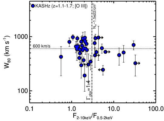
Figure 10: Emission-line width ($W_{80}$) versus the ratio between 2–10 keV and 0.5–2 keV X-ray fluxes for the 40 [O iii] detected KASH$z$ sample (circles). The X-ray axis here serves as a proxy for observed photon index ($\Gamma_{obs}$), and also as an estimate for obscuring column density (for an assumed intrinsic photon index and known redshift). We classify the sources with $F_{{\rm 2-10keV}}/F_{{\rm 0.5-2keV}}>3.03$ as “obscured candidates” (corresponding to $N_{H}\gtrsim$(1–2)$\times 10^{22}$ cm^-2; see Section 2.4). We find no evidence that high-velocity outflows are preferentially observed in the obscured X-ray AGN.

It has been suggested that massive galaxies may go through an evolutionary sequence where obscured AGN reside in star-forming galaxies during periods of rapid SMBH growth and galaxy growth during which the AGN drive outflows that drive away the enshrouding material to eventually reveal an unobscured AGN (e.g., Sanders et al. 1988; Hopkins et al. 2006). Therefore, it may be expected that outflows are more preferentially associated with X-ray obscured AGN. To test this, we compare the [O iii] emission-line velocities of our X-ray “obscured candidates” to those “unobscured candidates”, which we separate at an obscuring column density of $N_{H}\approx 2\times 10^{22}$ cm^-2 using a simple hard-band to soft-band flux ratio technique (see Section 2.4). In Figure 10 we show the emission-line velocity width, $W_{{\rm 80,[OIII]}}$, as a function of this flux ratio. We find no significant difference between the two populations; that is, we find that 45${}_{-9}^{+20}$ per cent of these sources have $W_{{\rm 80,[OIII]}}>600$ km s^-1, compared to a similar fraction of 54${}^{+15}_{-14}$ per cent for the unobscured sources. This result implies that high-velocity ionised outflows are certainly not uniquely, and do not appear to be preferentially, associated with X-ray obscured AGN. This may be in disagreement with some evolutionary scenarios for galaxy evolution; however, there may be a population of heavily obscured AGN that are missed from even the deepest X-ray surveys (see Section 2.3) that are not present in the current sample.

4.3.3 The prevalence and drivers of outflows observed in H$\alpha$

Figure 11: Stacked H$\alpha$+[N ii] emission-line profiles for the 25 Type 2 H$\alpha$ detected KASH$z$ targets and the comparison samples of: (1) star-forming galaxies at the same redshift and (2) $z<0.4$ Type 2 AGN (see Section 3.4). The dotted curves show the stacked data and the dashed and solid and dashed curves are fits to the stacks. The KASH$z$ AGN clearly show much broader emission-line profiles, and higher [N ii]/H$\alpha$ emission-line ratios than the star-forming galaxies.

In Figure 2 and Figure 3 we show the H$\alpha$+[N ii] emission-line profiles, and our best-fitting solutions, for all targets in the current $z$$\approx$0.6–1.1 KASH$z$ sample. The parameters for all of the fits are provided in Table 1. We detected 32 out of the 34 targets (see Section 4.1) and of these 32, we identified a BLR in seven of the targets (see Figure 3). For this study, we are interested in the kinematics of the host-galaxy, or equivalently the NLR, and not the BLR. Therefore, for these seven BLR sources the quoted emission-line velocity widths (i.e., the $W_{{\rm 80,H}\alpha}$), are for the NLR components only (see Section 3.2).

In Figure 11 we show the stacked H$\alpha$+[N ii] emission-line profile for our 25 H$\alpha$ Type 2 AGN. The overall-emission line width of this average profile is $W_{{\rm 80,H\alpha}}$=440${}^{+50}_{-13}$ km s^-1 (see Section 3.3), where the upper and lower bounds indicate the 68 per cent range from bootstrap resampling that stack. This velocity width is lower than the $W_{{\rm 80,[OIII]}}$=810${}^{+130}_{-220}$ km s^-1 observed in the stacked [O iii] emission-line profile (Figure 7). This difference is likely to be due, in part, to the almost order of magnitude difference in the average X-ray luminosity of the H$\alpha$ sample compared to the [O iii] sample (i.e., 2$\times$10⁴³ erg s^-1 compared to 1$\times$10⁴⁴ erg s^-1; see Figure 1), which we have shown be a key driver for the observed prevalence of high-velocity outflows (Section 4.3.2). However, as already briefly mentioned, this may also be due to these two emission lines preferentially tracing different regions of gas in the host galaxy, with H$\alpha$ likely to have a larger contribution from star-forming regions. While we currently lack systematic IFS studies of AGN covering both [O iii] and H$\alpha$ emission lines, observations of some AGN have already indicated that the NLR H$\alpha$ emission has a contribution from star-forming regions and is not necessarily dominated by the high-velocity outflows as is the case for [O iii] emission (e.g., Cano-Díaz et al. 2012; Cresci et al. 2015). Furthermore, a strong blue wing can be observed in the stacked KASH$z$ emission-line profile for the [N ii] emission-line, which has a larger velocity width than H$\alpha$ with $W_{{\rm 80,[NII]}}$=590${}^{+120}_{-50}$ km s^-1 (Figure 11). This high-ionisation line may be more analogous to the [O iii] emission, and preferentially trace outflowing/turbulent material compared to H$\alpha$. Indeed, the difficulty in identifying broad-underling outflow components in H$\alpha$ emission could be that this emission line preferentially traces rotation of the host galaxy and beam-smearing of this emission could dilute centrally-located broad components (Förster Schreiber et al. 2014; Genzel et al. 2014). We are unable to de-couple the [N II] from the H$\alpha$ across the whole H$\alpha$ sample due to limited signal-to-noise ratios (see Section 3.2) and therefore we may be underestimating the outflow velocities in these sources. However, H$\alpha$ emission has been used to identify outflows in AGN host-galaxies (e.g., Westmoquette et al. 2012; Arribas et al. 2014; Genzel et al. 2014) and analysis of this emission line using these methods provides an informative comparison to other studies.

In Figure 12 we show the distribution of the H$\alpha$ line-width values, $W_{80{\rm,H\alpha}}$, for the 32 detected targets, using the same format as above for the [O iii] emission. We find that four of our KASH$z$ targets (i.e., 13${}^{+9}_{-6}$ per cent) have $W_{{\rm 80,H}\alpha}>600$ km s^-1, indicative of emission that is dominated by outflowing material (see discussion at the start of this section). We note that the range on this percentage is 12–18 per cent if the two undetected targets are included, for which we have no constraints on $W_{{\rm 80,H}\alpha}$. In agreement with the [O iii] results (Section 4.3.1), we find no appreciable difference between the distribution of line-widths between the KASH$z$ sample and our low-redshift luminosity-matched comparison sample (see Section 3.4).

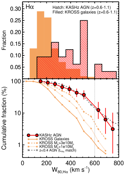
Figure 12: Top: Histograms of the overall emission-line velocity width, $W_{{\rm 80,H\alpha}}$, for the 32 $z$$\approx$0.6–1.1, H$\alpha$ detected KASH$z$ targets (hatched) and the $z$$\approx$0.6–1.1 comparison sample of star-forming galaxies from KROSS (filled; see Section 3.4). The AGN preferentially have higher emission-line velocities than the star-forming galaxies. This is further demonstrated in the bottom panel which show the cumulative distributions. We also show the KROSS sample after applying two stellar mass cuts, where the the $M_{\star}>3\times 10^{10}$ M_⊙ sub-sample is more comparable to the X-ray AGN host galaxies (Section 4.3.3). We also show the cumulative distribution of the luminosity-matched comparison sample of $z<0.4$ AGN (see Section 3.4) and find that the velocity distribution is very similar to that of our high-redshift AGN.

In Figure 12 we compare the H$\alpha$ emission-line velocity distributions for our KASH$z$ targets with our comparison sample of star-forming galaxies that are at the same redshift from KROSS (see Section 3.4). It can clearly be seen that AGN preferentially have higher emission-line widths than the star-forming galaxies. For example, only 3/378 (i.e., 0.8${}_{-0.4}^{+0.8}$ per cent) of the star-forming galaxy sample reach velocity-widths of $W_{{\rm 80,H}\alpha}>600$ km s^-1, compared to 13${}^{+9}_{-6}$ per cent found for the AGN. This is also demonstrated in Figure 11, where we show the stacked emission-line profiles for both samples. These results provide indirect evidence that the high-velocity features we observe are not pre-dominantly driven by star-formation. This is because X-ray AGN at these redshifts have average star-formation rates that are consistent with the global star-forming galaxy population of the same redshift (e.g., Rosario et al. 2012; Stanley et al. 2015), and are possibly even distributed to lower median star-formation rates (Mullaney et al. 2015). We further test this conclusion by plotting the velocity-width as a function of observed NLR H$\alpha$ luminosity ($L_{{\rm H\alpha,NLR}}$) for both the KASH$z$ sample and star-forming comparison sample in Figure 13. The observed NLR H$\alpha$ luminosity (i.e., excluding any BLR components) is a tracer of the star-formation rates in star-forming galaxies; however, for the AGN-host galaxies these will, in general be relative over-estimates due to the additional contribution of photoionisation by the central AGN. We find that the KASH$z$ AGN have a very similar distribution of $L_{{\rm H\alpha,NLR}}$ to our star-forming galaxy comparison sample, indicating that they have similar, or possibly lower star-formation rates. Despite this, the AGN-host galaxies preferentially have larger velocity widths, and a higher fraction of sources indicative of hosting high-velocity ionised outflows (Figure 13).

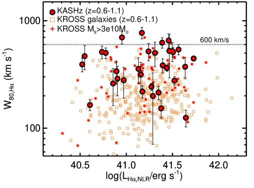
Figure 13: Emission-line velocity width, $W_{{\rm 80,H\alpha}}$ versus narrow-line region H$\alpha$ luminosity ($L_{{\rm H\alpha,NLR}}$) for the KASH$z$ AGN targets (circles) and the KROSS star-forming galaxies at the same redshift (squares). The AGN show a similar distribution of $L_{{\rm H\alpha,NLR}}$, but preferentially have the higher velocities. $L_{{\rm H\alpha,NLR}}$ is a tracer of the star-formation rates for the galaxies and the AGN (although this will be biased upwards for the AGN; see Section 4.3.3). Therefore, the higher emission-line velocities in the AGN are not the result of higher star-formation rates.

In addition to investigating the role of the star formation rates, it is also important to consider the effect of host galaxy masses on the H$\alpha$ emission-line widths. In the cases where the H$\alpha$ emission-line profiles are dominated by galaxy kinematics (which is the case for the majority of the star-forming KROSS galaxies; e.g., Stott et al. 2015; Swinbank et al. in prep), the line-widths will be driven to higher values in galaxies with higher stellar masses due to the increased velocity gradients across these galaxies. To demonstrate this, in Figure 12, we also show the cumulative distributions of line-widths for the star-forming galaxies when we apply increasing mass cuts. As expected, the higher mass galaxies tend to have the broader emission-line widths. We do not attempt to derive stellar masses for our AGN, due to the variable quality of photometric data sets available for our targets; however, we note that X-ray AGN appear to typically have stellar masses of $\gtrsim 3\times$10¹⁰ M_⊙ (e.g., Mullaney et al. 2012; Bongiorno et al. 2012; Aird et al. 2013; Azadi et al. 2015). Therefore, in Figure 12, we compare the star-forming galaxy sample, but limiting it to galaxies with stellar masses $>3\times$10¹⁰ M_⊙. We still find that the KASH$z$ AGN have a higher prevalence of the highest velocity widths, compared to this higher mass subset of the star-forming galaxies, with only 3${}^{+6}_{-1}$ per cent exhibiting emission-line velocity widths of $W_{{\rm 80,H}\alpha}>600$ km s^-1.

To further test the possible role of mass in driving the high emission-line velocity widths observed in our targets, in Figure 14 we plot $W_{{\rm 80,H}\alpha}$ as a function of the emission-line ratio $\log$([N ii]/H$\alpha$). This emission-line ratio is a tracer of the metallicity of star-forming galaxies (e.g., Alloin et al. 1979; Denicoló et al. 2002; Kewley & Dopita 2002), as well as an indicator for the source of ionising radiation (e.g. Kewley et al. 2006; Rich et al. 2014). Furthermore, there is an observed relationship between mass and metallicity and therefore an expected relationship between this emission-line ratio and stellar mass (e.g., Lequeux et al. 1979; Tremonti et al. 2004; Maiolino et al. 2008; Stott et al. 2013). We can also make a crude prediction for the relationship between $W_{{\rm 80,H}\alpha}$ and mass, under the assumption that the line-width is a tracer of the stellar velocity dispersion. Therefore, for a given stellar mass, we predict the position galaxies would be located in Figure 14 by combining: (1) the observed $z=0.7$ mass-metallicity relation (following Maiolino et al. 2008) and (2) the observed mass-velocity dispersion relationship for massive galaxies (following Bezanson et al. 2015). The majority of the star-forming galaxies appear to broadly follow the expected trend. Furthermore, the measurements from the stacked average emission-line profile (Figure 11) are in agreement with the rough mass-driven prediction for the average mass of these galaxies (i.e., $\log(M_{\star}/M_{\odot})$=10.3; see Figure 14). In contrast, the AGN typically have higher $\log$([N ii]/H$\alpha$) emission-line ratios and higher velocity widths that the star-forming galaxy sample (also visible in the stacked profiles; Figure 11) and a positive correlation is observed between these two quantities. Such a positive correlation has been shown to be a tracer of shocks and outflows in the ISM through IFS observations of AGN and star-forming galaxies (e.g., Ho et al. 2014; McElroy et al. 2015). Interestingly, the small number of star-forming galaxies with high line-widths (i.e., $W_{80}\gtrsim 400$ km s^-1) appear to follow the same relationship as the KASH$z$ AGN, which may indicate that these galaxies also have a contribution from shocks and/or host AGN that were not detected in the X-ray surveys. We clarify that some of the AGN targets have $\log$([N ii]/H$\alpha$) emission-line ratios that could also be photoionised by H ii regions (see Figure 14) and we will explore these ideas further when exploring the spatially-resolved outflow kinematics and emission-line flux ratios of the KASH$z$ AGN in future papers.

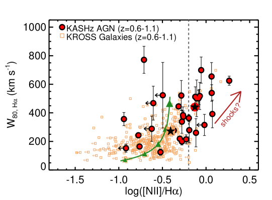
Figure 14: Emission-line velocity width, $W_{{\rm 80,H\alpha}}$ versus $\log$([N ii]/H$\alpha_{\rm NLR}$) emission-line ratio for the KASH$z$ AGN targets (circles) and the KROSS star-forming galaxies (squares). The larger symbols containing the stars are measured from the stacked emission-line profiles (Figure 11). The vertical dashed line indicates the maximum emission-line ratio expected for photoionised H ii regions (e.g., Kewley et al. 2013). The green track shows the predicted trends as a function of mass (following the mass-metallicity and mass-velocity dispersion relations; see Section 4.3.3), where the triangles highlight various $\log(M_{\star})$ values in half dex bins starting at 9.0. The positive correlation observed for most of the AGN (i.e., those with $\log$([N ii]/H$\alpha$)$\gtrsim$$-0.5$ may be indicative of outflows/shocks driving the velocity widths (see Section 4.3.3). Most of the star-forming galaxies roughly follow the predicted mass-driven trend (Section 3.4) and the stacked average is consistent with the mass-driven prediction at their average mass, i.e., $\log(M_{\star}/M_{\odot})$=10.3. However, they appear to follow the same trend as the AGN at the largest velocity widths ($W_{80}\gtrsim$400 km s^-1).

We conclude that the highest H$\alpha$ line-widths (i.e., those with $W_{80}>600$ km s^-1 and possibly those with $W_{80}\gtrsim 400$ km s^-1) are at least partially driven by ionised outflow kinematics and/or shocks in the ISM. Furthermore, there is a increased likelihood to find these highest ionised gas velocities in X-ray identified AGN compared to star-forming galaxies at the same redshift that have similar star-formation rates and masses. This is in agreement with local IFS studies that have found higher-velocity ionised outflows, traced by H$\alpha$ emission, in star-forming galaxies that host AGN compared to those which do not (e.g., Westmoquette et al. 2012; Arribas et al. 2014).

5 Conclusions

We have presented the first results of the ongoing KMOS AGN Survey at High redshift (KASH$z$). The first 89 targets, which are presented here, are high-redshift ($z$$\approx$0.6–1.7) X-ray detected AGN, with hard-band (2–10 keV) luminosities in the range $L_{{\rm X}}=10^{42}$–10⁴⁵ erg s^-1. The targets have a distribution of X-ray luminosities that are representative of the parent X-ray AGN population. The majority of the targets (79) were observed with KMOS, supplemented with archival SINFONI observations of 10 targets. All of the observations were carried out in the $J$-band and we detected 86 (i.e., 97 per cent) of the targets in continuum and/or emission lines. However, for the analyses in this work, we excluded seven un-reliable non-detections (e.g., due to inaccurate photometric redshifts; Section 4.1). This leaves a final sample of 82 targets, for which we have presented results and discussion based on their galaxy-integrated emission-line profiles.

We detected 72 of the final sample (i.e., 88 per cent) in emission lines, of which 40 out of 48 targets were detected in [O iii] (the $z$$\approx$1.1–1.7 targets) and 32 out of 34 targets were detected in H$\alpha$ (the $z$$\approx$0.6–1.1 targets). We have explored the emission-line luminosities as a function of X-ray luminosity for our targets and by characterising the individual emission-line profiles and using stacking analyses, we have investigated the prevalence and drivers of the broad and asymmetric emission-line profiles that are indicative of ionised outflows. Our main conclusions are listed below.

• We find a median X-ray luminosity to [O iii] luminosity ratio of $\log(L_{{\rm[O~{}III}]}/L_{X})=-2.1_{-0.5}^{+0.3}$, where the range is roughly the 1$\sigma$ scatter. The observed relationship between these two quantities for our high-redshift sample is broadly consistent with that found for low-redshift AGN and local Seyferts and QSOs (see Figure 5). Our results indicate that the [O iii] luminosities are typically $\approx$1% of the X-ray luminosities for $z\approx$1.1–1.7 X-ray AGN. The large scatter of a factor of $\approx$3, may be due to several observational effects including dust reddening, or due to intrinsic physical effects, such as a higher level of variability in the sub-pc-scale production X-ray emission compared to the kpc-scale production of [O iii] emission (Section 4.2).

• Our seven Type 1 H$\alpha$ targets have broad-line region luminosities ($L_{{\rm H\alpha,BLR}}$) that are broadly consistent with the correlation observed between $L_{{\rm H\alpha,BLR}}$ and $L_{X}$ for low-redshift and local AGN. Although limited by small numbers of very luminous sources, we find no evidence for a correlation between the narrow-line region H$\alpha$ luminosity and $L_{X}$ (see Figure 6; Section 4.2).

• High-velocity emission-line features are common in our [O iii] sample, with $\approx$50 per cent of the targets exhibiting velocities indicative of being dominated by outflowing ionised gas or highly turbulent material (i.e., emission-line velocity widths of $W_{{\rm 80,[OIII]}}$$>$600 km s^-1; see Figure 7; Figure 8 and Section 4.3.1). On average the emission-line profiles have a prominent blue-shifted wing, implying outflowing material. Outflowing or highly turbulent material that does not dominate the individual emission-line profiles could be even more common.

• The high-velocity [O iii] kinematics are more prevalent for targets with higher AGN luminosities. For example, $\approx$70 per cent of the $L_{X}>6\times 10^{43}$ erg s^-1 targets have [O iii] line widths of $W_{{\rm 80,[OIII]}}$$>$600 km s^-1, while only $\approx$30 per cent of the $L_{X}<6\times 10^{43}$ erg s^-1 targets reach these line widths (see Figure 8 and Figure 9). Using our current sample, we are unable to determine the role of radio luminosity in driving this trend (Section 4.3.2).

• Based on our current X-ray detected sample, we find no evidence that the highest ionised gas velocities are preferentially associated with X-ray obscured AGN (i.e., those with $N_{H}\gtrsim 10^{22}$ cm^-2), compared to X-ray unobscured AGN (see Figure 10), in contrast to the predictions of some evolutionary scenarios (Section 4.3.2).

• We compared the emission-line widths of our H$\alpha$ detected X-ray AGN targets, with a redshift matched sample of star-forming galaxies. Despite a similar distribution of H$\alpha$ luminosities (excluding the broad-line region components), and implied similar star-formation rates, the AGN-host galaxies exhibit a much higher prevalence of high ionised gas velocities (see Figure 12 and Figure 11). For example, $\approx$13 per cent of the AGN have H$\alpha$ emission-line widths of $W_{80}>$600 km s^-1, whilst only $\approx$1 per cent of the star-forming galaxy sample reach these line widths (Section 4.3.3).

• For both the [O iii] and H$\alpha$ KASH$z$ targets, we find no significant difference between the distribution of velocity widths for our high-redshift AGN sample and luminosity-matched comparison samples of $z<0.4$ AGN. Under the assumption that the most extreme ionised gas velocities are associated with outflows, to first order, this implies that it is just as likely to find an ionised outflow of a certain velocity in low-redshift AGN as in high-redshift AGN of the same luminosities (see Figure 8 and Figure 12). This is despite the order-of-magnitude global decrease in average star-formation rates towards the lower redshift sample (see Section 4.3.1 and Section 4.3.3).

Based on our systematic study of a representative sample of high-redshift X-ray detected AGN, we have evidence that high-velocity ionised outflows are prevalent, in qualitative agreement with theoretical predictions of galaxy formation models. These features appear to be most common in the most powerful AGN, and are equally prevalent in the high-redshift Universe as in the low-redshift Universe for AGN of the same luminosity. Our analyses focused on searching for emission-line profiles which are dominated by these extreme gas kinematics and lower level outflows or highly turbulent material could be even more common. Due to a higher fraction of galaxies hosting the most luminous AGN at higher redshifts, our results imply that the most extreme ionised outflows are more prevalent in high-redshift galaxies. In future papers, we will present results based on the spatially-resolved kinematics of multiple emission lines which will reveal information on the sizes and morphologies of the high-velocity gas, enable us to disentangle outflows from galaxy kinematics, and to measure the energetics of the outflows (following e.g., Nesvadba et al. 2008; Harrison et al. 2012; Harrison et al. 2014; Cano-Díaz et al. 2012; Cresci et al. 2015). Furthermore, as our sample size grows, we will be able to make more definitive tests on the drivers and impact of ionised outflows in large samples of representative AGN.

Acknowledgements

We thank the referee for their constructive comments. We acknowledge the Science and Technology Facilities Council (CMH, DMA, JPS, AMS, RGB and RMS through grant code ST/L00075X/1) and the Leverhulme Trust (DMA). JRM acknowledges support from the University of Sheffield via its Vice-Chancellor Fellowship scheme. JPS acknowledges support from a Hintze Research Fellowship. FEB acknowledges support from CONICYT-Chile (Basal-CATA PFB-06/2007, FONDECYT 1141218, “EMBIGGEN” Anillo ACT1101), and Project IC120009 “Millennium Institute of Astrophysics (MAS)” funded by the Iniciativa Científica Milenio del Ministerio de Economía, Fomento y Turismo. We thank the members of the KROSS team for access to their data and for assisting with KASH$z$ observations. We also thank Holly Elbert and Timothy Green for carrying out some observations. We thank F. Stanley for providing star formation rate measurements and Ian Smail for useful discussions.

Appendix A Emission-line profiles and tabulated data

In this Appendix we provide the galaxy-integrated spectra, emission-line profile fits and tabulated data for all 89 of the KASH$z$ targets presented in this work.

KASH$z$ Target Properties

Name	$z_{A}$	Type	$F_{{\rm 0.5-2}}$	$F_{{\rm 2-10}}$	Obs.	RL	Inst.	Line	te	Note	BLR	$z_{L}$	$S_{A}$	FWA	$S_{B}$	FWB	$\Delta v$	$S_{{\rm[NII]}}$	$W_{80}$
(1)	(2)	(3)	(4)	(5)	(6)	(7)	(8)	(9)	(10)	(11)	(12)	(13)	(14)	(15)	(16)	(17)	(18)	(19)	(20)
UDS-186	1.437	s	4.07	5.06	U	✗	K	O	9.0	C	-	-	$<$0.7	-	-	-	-	-	-
UDS-310	1.645	s	6.96	14.15	U	✗	K	O	5.4	L	-	1.645	1.8$\pm$0.7	176$\pm$86	-	-	-	-	192$\pm$94
UDS-357	1.100	s	16.16	33.18	U	✗	K	O	5.4	L	$\beta$	1.098	4.5$\pm$1.0	779$\pm$154	-	-	-	-	848$\pm$168
UDS-574	1.533	s	4.55	4.51	U	✗	K	O	6.0	C	-	-	$<$0.9	-	-	-	-	-	-
UDS-584	1.602	s	2.74	5.22	U	✗	K	O	9.0	L	-	1.605	4.5$\pm$0.8	107$\pm$26	25.0$\pm$1.1	611$\pm$28	-52$\pm$13	-	615$\pm$26
UDS-586	1.171	s	11.97	16.01	U	✗	K	O	6.0	L	-	1.171	2.3$\pm$0.3	575$\pm$83	-	-	-	-	625$\pm$90
UDS-605	1.096	s	2.77	9.76	O	✗	K	O	6.0	L	-	1.097	1.7$\pm$0.7	696$\pm$253	-	-	-	-	758$\pm$276
UDS-619	1.410	s	19.18	35.01	U	✗	K	O	6.0	L	$\beta$	1.401	21.2$\pm$4.9	242$\pm$29	33.8$\pm$4.3	666$\pm$68	-18$\pm$15	-	562$\pm$33
UDS-631	1.192	s	3.79	10.70	U	✗	K	O	8.4	L	-	1.190	1.6$\pm$0.4	318$\pm$95	-	-	-	-	346$\pm$104
UDS-640	1.092	s	6.61	10.32	U	✗	K	O	6.0	L	-	1.093	5.4$\pm$0.3	523$\pm$36	-	-	-	-	570$\pm$39
UDS-643	1.087	s	3.46	5.45	U	✗	K	O	6.0	L	$\beta$	1.088	2.4$\pm$0.7	146$\pm$66	2.8$\pm$0.9	565$\pm$149	-189$\pm$121	-	492$\pm$161
UDS-655	1.397	s	4.92	8.32	U	✗	K	O	6.0	L	-	1.397	1.5$\pm$0.6	272$\pm$114	-	-	-	-	297$\pm$125
UDS-671	1.083	s	0.27	8.02	O	✗	K	O	6.0	L	-	1.084	0.8$\pm$0.5	77$\pm$66	3.6$\pm$0.8	712$\pm$176	-191$\pm$90	-	702$\pm$134
UDS-676	1.086	s	3.41	1.91	U	✗	K	O	9.0	L	-	1.086	0.7$\pm$0.3	389$\pm$215	-	-	-	-	424$\pm$235
UDS-701	1.653	s	1.45	3.35	U	✗	K	O	9.0	L	-	1.649	2.1$\pm$1.1	520$\pm$268	-	-	-	-	566$\pm$291
UDS-763	1.413	s	18.88	26.59	U	✗	K	O	9.0	L	$\beta$	1.412	5.4$\pm$3.0	261$\pm$78	12.3$\pm$3.3	705$\pm$142	-168$\pm$90	-	668$\pm$84
UDS-796	1.132	s	3.80	29.03	O	✗	K	O	9.0	C	-	-	$<$1.7	-	-	-	-	-	-
UDS-814	1.074	s	25.01	22.10	U	✗	K	O	9.0	L	-	1.077	3.1$\pm$0.5	735$\pm$133	-	-	-	-	800$\pm$144
UDS-855	1.407	s	5.19	20.10	O	✓	K	O	8.4	L	-	1.407	11.4$\pm$1.1	475$\pm$45	-	-	-	-	517$\pm$49
COS-20	1.156	s	1.34	7.01	O	✓	K	O	9.6	L	-	1.154	1.7$\pm$0.5	324$\pm$130	0.9$\pm$0.6	380$\pm$214	381$\pm$25	-	612$\pm$120
COS-27⋆	1.510	p	$<$0.73	2.59	O	✗	K	O	5.4	C	-	-	-	-	-	-	-	-	-
COS-40	1.510	s	4.69	9.69	U	✗	K	O	9.0	L	-	1.504	2.8$\pm$1.3	485$\pm$171	2.8$\pm$1.6	1277$\pm$375	0$\pm$72	-	953$\pm$273
COS-61	1.478	s	1.45	4.41$\dagger$	?	✗	K	O	8.4	L	-	1.478	3.5$\pm$0.6	225$\pm$45	-	-	-	-	245$\pm$49
COS-108	1.253	s	4.39	16.10	O	✓	S	O	12.0	L	-	1.258	25.6$\pm$3.0	331$\pm$26	10.9$\pm$4.6	1360$\pm$409	-506$\pm$220	-	936$\pm$170
COS-178	1.347	s	1.47	8.92	O	✗	S	O	12.0	C	-	-	$<$1.2	-	-	-	-	-	-
COS-203	1.360	s	7.37	14.20	U	✗	K	O	7.2	L	-	1.359	5.1$\pm$0.6	337$\pm$49	-	-	-	-	367$\pm$53
COS-206	1.483	s	5.89	10.40	U	✗	K	O	7.2	L	$\beta$	1.480	3.8$\pm$2.0	630$\pm$323	-	-	-	-	685$\pm$352
COS-211	1.166	s	2.65	4.12	U	✗	K	O	7.2	L	-	1.167	2.4$\pm$0.5	535$\pm$113	-	-	-	-	582$\pm$123
COS-453	1.625	s	3.01	5.70	U	✓	K	O	9.0	C	-	-	$<$0.5	-	-	-	-	-	-
COS-454	1.478	s	5.91	10.90	U	✗	K	O	9.0	L	$\beta$	1.484	2.5$\pm$1.3	250$\pm$110	3.9$\pm$1.9	827$\pm$415	-480$\pm$198	-	922$\pm$280
COS-499	1.459	s	27.40	57.80	U	✓	K	O	9.0	L	$\beta$	1.455	3.6$\pm$1.2	165$\pm$49	22.1$\pm$1.7	786$\pm$58	-109$\pm$28	-	796$\pm$52
COS-649	1.369	s	$<$1.05	3.77	O	✗	K	O	5.4	L	-	1.367	2.0$\pm$0.7	415$\pm$166	-	-	-	-	451$\pm$180
COS-832⋆	1.471	p	$<$0.86	2.71	O	✓	K	O	8.4	C	-	-	-	-	-	-	-	-	-
COS-885⋆	1.594	p	0.44	1.34$\dagger$	?	✗	K	O	9.0	C	-	-	-	-	-	-	-	-	-
COS-1015	1.379	s	1.14	3.47$\dagger$	U	✗	K	O	7.2	L	-	1.377	1.4$\pm$0.6	281$\pm$160	-	-	-	-	306$\pm$174
COS-1518⋆	1.122	s	$<$0.24	2.90	O	✗	K	O	9.6	N	-	-	-	-	-	-	-	-	-
COS-3178	1.355	s	$<$0.59	2.54	O	✗	K	O	7.2	L	-	1.354	3.6$\pm$2.3	882$\pm$547	-	-	-	-	960$\pm$596
COS-3715	1.103	s	0.36	1.11$\dagger$	?	✗	K	O	5.4	C	-	-	$<$0.7	-	-	-	-	-	-
XCOS-2028	1.592	s	33.50	75.70	U	✓	S	O	25.2	L	$\beta$	1.593	17.3$\pm$5.1	410$\pm$36	16.4$\pm$5.4	657$\pm$88	-332$\pm$76	-	734$\pm$17
XCOS-5627	1.337	s	7.25	15.40	U	✗	S	O	12.6	L	$\beta$	1.349	0.7$\pm$0.7	62$\pm$62	9.0$\pm$2.1	573$\pm$191	-5$\pm$14	-	602$\pm$131
CDFS-25	1.374	s	$<$0.19	1.21	O	✗	K	O	6.0	L	-	1.377	3.5$\pm$2.1	184$\pm$51	9.7$\pm$2.4	518$\pm$94	-183$\pm$64	-	524$\pm$37

Table 1: Continued over page.

KASH$z$ Target Properties (continued)

Name	$z_{A}$	Type	$F_{{\rm 0.5-2}}$	$F_{{\rm 2-10}}$	Obs.	RL	Inst.	Line	te	Note	BLR	$z_{L}$	$S_{A}$	FWA	$S_{B}$	FWB	$\Delta v$	$S_{{\rm[NII]}}$	$W_{80}$
(1)	(2)	(3)	(4)	(5)	(6)	(7)	(8)	(9)	(10)	(11)	(12)	(13)	(14)	(15)	(16)	(17)	(18)	(19)	(20)
CDFS-88	1.616	s	3.07	4.67	U	✗	K	O	9.0	C	-	-	$<$0.7	-	-	-	-	-	-
CDFS-113⋆	1.608	i	0.57	0.98	U	✗	K	O	9.0	N	-	-	-	-	-	-	-	-	-
CDFS-166	1.605	s	8.14	12.39	U	✓	K	O	9.0	L	-	1.611	5.7$\pm$0.4	371$\pm$25	-	-	-	-	404$\pm$27
CDFS-191	1.185	s	$<$0.13	4.18	O	✗	K	O	6.0	L	-	1.184	1.8$\pm$0.6	297$\pm$125	-	-	-	-	323$\pm$136
CDFS-243	1.097	s	0.71	12.29	O	✗	K	O	6.0	L	-	1.096	2.5$\pm$0.8	468$\pm$160	-	-	-	-	510$\pm$174
CDFS-343	1.090	s	$<$0.08	1.46	O	✗	K	O	9.6	C	-	-	$<$0.4	-	-	-	-	-	-
CDFS-344	1.617	s	3.64	3.89	U	✓	K	O	7.8	L	-	1.613	3.7$\pm$0.9	258$\pm$40	7.4$\pm$1.4	1089$\pm$149	-270$\pm$83	-	977$\pm$112
CDFS-518	1.603	s	9.74	13.30	U	✓	K	O	9.6	L	-	1.609	8.3$\pm$1.0	850$\pm$88	-	-	-	-	926$\pm$96
CDFS-549⋆	1.553	s	1.36	3.25	U	✗	K	O	11.4	N	-	-	-	-	-	-	-	-	-
CDFS-619	1.178	s	0.16	2.17	O	✗	K	O	7.8	L	-	1.179	1.6$\pm$0.6	419$\pm$147	-	-	-	-	457$\pm$160
CDFS-720	1.609	s	10.93	18.44	U	✗	K	O	9.0	L	-	1.610	2.2$\pm$0.5	742$\pm$173	-	-	-	-	808$\pm$189
SSA22-39	1.397	s	7.19	9.08	U	?	S	O	3.0	L	-	1.400	8.2$\pm$1.8	605$\pm$143	-	-	-	-	658$\pm$156
SSA22-141	1.370	s	20.53	27.38	U	?	S	O	2.4	L	-	1.367	5.4$\pm$2.2	541$\pm$209	-	-	-	-	589$\pm$227
UDS-194	0.627	s	5.80	10.13	U	✗	K	H	9.0	L	$\alpha$	0.628	8.1$\pm$0.9	328$\pm$42	25.2$\pm$2.3	5385$\pm$604	258$\pm$190	0.93	357$\pm$46
UDS-275	0.883	s	7.27	52.96	O	✗	K	H	5.4	L	-	0.882	4.5$\pm$0.9	476$\pm$87	-	-	-	3.85	518$\pm$95
UDS-393	0.822	s	9.70	9.38	U	✗	K	H	9.0	L	$\alpha$	0.822	6.0$\pm$0.5	183$\pm$22	49.1$\pm$3.4	5811$\pm$457	176$\pm$164	3.18	199$\pm$24
UDS-403	1.021	s	2.30	13.81	O	✗	K	H	9.0	L	-	1.021	3.7$\pm$0.9	461$\pm$118	-	-	-	2.89	502$\pm$129
UDS-600	0.873	s	4.41	4.34	U	✗	K	H	6.0	L	$\alpha$	0.873	11.6$\pm$1.3	343$\pm$36	29.2$\pm$3.1	2401$\pm$216	-158$\pm$108	6.39	373$\pm$39
UDS-620	0.842	s	1.08	3.44	O	✗	K	H	9.0	L	-	0.843	2.3$\pm$0.4	311$\pm$75	-	-	-	1.21	338$\pm$81
UDS-818	0.928	s	14.55	19.28	U	✗	K	H	8.4	L	-	0.928	5.5$\pm$0.6	140$\pm$26	-	-	-	$<$0.66	153$\pm$29
UDS-827	0.658	s	4.65	12.22	U	✗	K	H	8.4	L	$\alpha$	0.657	8.0$\pm$0.4	201$\pm$15	22.7$\pm$2.1	5129$\pm$548	682$\pm$196	4.02	219$\pm$17
UDS-862	0.589	s	1.35	8.50	O	✗	K	H	8.4	L	-	0.589	3.8$\pm$0.5	471$\pm$64	-	-	-	2.88	512$\pm$70
UDS-883	0.961	s	24.39	56.58	U	✗	K	H	8.4	L	$\alpha$	0.961	5.2$\pm$0.4	574$\pm$29	30.5$\pm$2.9	7970$\pm$795	-748$\pm$271	9.50	625$\pm$32
COS-44	1.513	p	1.23	3.56	U	✗	K	H	9.0	L	-	0.801	4.9$\pm$0.4	709$\pm$87	-	-	-	0.95	771$\pm$95
COS-401	0.969	s	$<$1.14	13.30	O	✓	S	H	2.4	L	-	0.971	7.6$\pm$0.9	495$\pm$53	-	-	-	8.80	539$\pm$58
COS-724	0.906	s	$<$0.51	4.04	O	✗	K	H	6.0	C	-	-	$<$1.2	-	-	-	-	-	-
COS-829	0.885	s	0.39	1.17$\dagger$	?	✗	K	H	8.4	L	-	0.885	6.4$\pm$0.8	353$\pm$53	-	-	-	3.50	384$\pm$57
COS-932	0.975	s	0.71	2.17$\dagger$	U	✗	K	H	8.4	L	-	0.974	6.5$\pm$0.6	469$\pm$49	-	-	-	5.46	511$\pm$53
COS-1070⋆	0.858	p	1.06	2.30	U	✗	K	H	8.4	C	-	-	-	-	-	-	-	-	-
COS-1157	0.915	s	0.49	1.50$\dagger$	?	✗	K	H	9.6	L	-	0.925	5.2$\pm$0.6	197$\pm$29	-	-	-	3.07	215$\pm$31
COS-1199	0.771	p	0.67	2.10	O	✗	K	H	9.0	L	-	0.850	9.5$\pm$0.7	255$\pm$23	-	-	-	4.05	277$\pm$25
CDFS-51	0.737	s	1.81	18.33	O	✗	S	H	2.7	L	-	0.737	11.9$\pm$3.5	481$\pm$211	-	-	-	$<$3.79	523$\pm$230
CDFS-101	0.977	s	11.57	20.66	U	✗	K	H	9.0	L	$\alpha$	0.978	2.9$\pm$0.5	290$\pm$68	133.5$\pm$3.7	7150$\pm$202	-843$\pm$77	$<$2.78	315$\pm$74
CDFS-356	1.034	s	0.29	0.57	U	✗	K	H	6.0	L	-	1.034	3.3$\pm$0.2	223$\pm$17	-	-	-	0.55	243$\pm$19
CDFS-370	0.734	s	1.07	3.38	O	✗	S	H	2.7	C	-	-	$<$3.8	-	-	-	-	-	-
CDFS-433	0.617	s	1.04	2.03	U	✗	K	H	9.6	L	-	0.620	3.7$\pm$0.4	461$\pm$52	-	-	-	3.03	501$\pm$57
CDFS-454	0.952	i	1.42	3.17	U	✗	K	H	11.4	L	-	0.953	2.0$\pm$0.5	257$\pm$82	-	-	-	1.30	279$\pm$89
CDFS-480	0.839	s	2.48	4.08	U	✗	K	H	6.0	L	-	0.841	7.3$\pm$2.1	286$\pm$41	2.0$\pm$2.1	427$\pm$280	-367$\pm$169	4.80	521$\pm$105
CDFS-492	0.735	s	0.13	2.55	O	✗	S	H	5.4	L	-	0.735	11.2$\pm$0.6	334$\pm$22	-	-	-	7.13	363$\pm$24
CDFS-506	0.665	s	4.30	7.35	U	✗	K	H	7.8	L	-	0.666	1.8$\pm$0.4	430$\pm$109	-	-	-	$<$0.46	468$\pm$119

Table 1: Continued over page.

KASH$z$ Target Properties (continued)

Name	$z_{A}$	Type	$F_{{\rm 0.5-2}}$	$F_{{\rm 2-10}}$	Obs.	RL	Inst.	Line	te	Note	BLR	$z_{L}$	$S_{A}$	FWA	$S_{B}$	FWB	$\Delta v$	$S_{{\rm[NII]}}$	$W_{80}$
(1)	(2)	(3)	(4)	(5)	(6)	(7)	(8)	(9)	(10)	(11)	(12)	(13)	(14)	(15)	(16)	(17)	(18)	(19)	(20)
CDFS-514	0.664	s	3.29	4.49	U	✗	K	H	7.8	L	-	0.667	4.2$\pm$0.8	265$\pm$81	-	-	-	$<$0.99	289$\pm$88
CDFS-561	0.798	s	0.08	2.69	O	✗	K	H	7.8	L	-	0.980	1.4$\pm$0.4	239$\pm$91	-	-	-	1.11	261$\pm$99
CDFS-592	1.016	s	0.69	4.03	O	✗	K	H	9.0	L	-	1.015	5.3$\pm$0.9	601$\pm$89	-	-	-	6.13	655$\pm$97
CDFS-606	0.733	s	0.34	2.58	O	✗	K	H	7.8	L	-	0.733	1.7$\pm$0.2	151$\pm$17	-	-	-	0.29	164$\pm$19
CDFS-614	0.668	s	0.38	0.86	U	✗	K	H	9.0	L	-	0.667	4.7$\pm$0.5	642$\pm$84	-	-	-	4.09	699$\pm$92
CDFS-629	0.667	s	0.83	2.60	O	✗	K	H	9.0	L	$\alpha$	0.667	1.7$\pm$0.5	360$\pm$89	30.1$\pm$6.3	9647$\pm$1706	-846$\pm$549	2.04	392$\pm$97
CDFS-652	1.020	s	0.66	1.18	U	✗	K	H	7.8	L	-	1.022	8.0$\pm$0.7	115$\pm$21	-	-	-	2.40	125$\pm$22
CDFS-706	0.891	s	$<$0.15	1.02	O	✗	K	H	9.0	L	-	0.890	13.7$\pm$0.4	409$\pm$16	-	-	-	6.63	445$\pm$18

Table 1: Properties for the KASH$z$ targets observed so far. Notes: (1) Source name (‘field’ – ‘X-ray ID’), those targets followed by a ^⋆ are excluded from the analyses presented in this paper (see Section 4.1); (2) archival redshift; (3) archival redshift type (i.e., photometric [p], secure spectroscopic redshift [s] or insecure spectroscopic redshift [i]); (4) and (5) soft-band (0.5–2 keV) and hard-band (2–10 keV) X-ray fluxes ($\times$10^-15 erg s^-1 cm ^-2), where the hard-band values followed by a $\dagger$ were estimated from the soft-band fluxes (see Section 2.1); (6) flag to indicate X-ray obscured candidates (O) and unobscured candidates (U), those without sufficient constraints are labelled with “?”; (7) flag to indicate the “radio luminous” targets with $L_{{\rm 1.4GHz}}>10^{24}$ W Hz^-1 (Section 2.5); (8) instrument used for the observations (K$=$KMOS and S$=$SINFONI); (9) primary targeted emission line (O$=$[O iii] and H$=$H$\alpha$); (10) on-source exposure time (kilo-seconds); (11) note on data (L$=$line detected; C$=$ continuum only detected; N$=$no detection); (12) note for the identification of a BLR component ($\alpha$ for H$\alpha$ and $\beta$ for H$\beta$); (13) redshift derived from the narrowest Gaussian component of the emission-line profile fit; (14) and (15) Flux ($\times 10^{-17}$ erg s^-1 cm^-2) and FWHM (km s^-1) of the narrower Gaussian component; (16) and (17) Flux ($\times 10^{-17}$ erg s^-1 cm^-2) and FWHM of the broader Gaussian component (for sources with “$\alpha$” in column 10, this is the BLR component); (18) velocity offset between the two Gaussian components (km s^-1); (19) flux of [N ii]$\lambda$6583 ($\times 10^{-17}$ erg s^-1 cm^-2) where applicable; (20) overall emission-line width (km s^-1). All of the quoted uncertainties are the random errors on the fits due to the noise in the spectra; however, we note that throughout this work we add an extra 30% systematic error to the emission-line fluxes to account for the uncertainty in the flux calibration (see Section 3.2).

References

- Abazajian et al. (2009) Abazajian K. N. et al., 2009, ApJS, 182, 543
- Aird et al. (2013) Aird J. et al., 2013, ApJ, 775, 41
- Aird et al. (2010) Aird J. et al., 2010, MNRAS, 401, 2531
- Alexander et al. (2008) Alexander D. M. et al., 2008, ApJ, 687, 835
- Alexander & Hickox (2012) Alexander D. M., Hickox R. C., 2012, New Astron. Rev., 56, 93
- Alexander et al. (2010) Alexander D. M., Swinbank A. M., Smail I., McDermid R., Nesvadba N. P. H., 2010, MNRAS, 402, 2211
- Alloin et al. (1979) Alloin D., Collin-Souffrin S., Joly M., Vigroux L., 1979, A&A, 78, 200
- Arribas et al. (2014) Arribas S., Colina L., Bellocchi E., Maiolino R., Villar-Martín M., 2014, A&A, 568, A14
- Azadi et al. (2015) Azadi M. et al., 2015, ApJ, 806, 187
- Baldry et al. (2012) Baldry I. K. et al., 2012, MNRAS, 421, 621
- Balmaverde et al. (2015) Balmaverde B. et al., 2015, arXiv:1506.05984
- Barth et al. (2008) Barth A. J., Greene J. E., Ho L. C., 2008, AJ, 136, 1179
- Benson et al. (2003) Benson A. J., Bower R. G., Frenk C. S., Lacey C. G., Baugh C. M., Cole S., 2003, ApJ, 599, 38
- Berney et al. (2015) Berney S. et al., 2015, MNRAS, 454, 3622
- Bezanson et al. (2015) Bezanson R., Franx M., van Dokkum P. G., 2015, ApJ, 799, 148
- Bongiorno et al. (2012) Bongiorno A. et al., 2012, MNRAS, 427, 3103
- Bonzini et al. (2013) Bonzini M., Padovani P., Mainieri V., Kellermann K. I., Miller N., Rosati P., Tozzi P., Vattakunnel S., 2013, MNRAS, 436, 3759
- Boroson et al. (1985) Boroson T. A., Persson S. E., Oke J. B., 1985, ApJ, 293, 120
- Bower et al. (2006) Bower R. G., Benson A. J., Malbon R., Helly J. C., Frenk C. S., Baugh C. M., Cole S., Lacey C. G., 2006, MNRAS, 370, 645
- Bower et al. (2008) Bower R. G., McCarthy I. G., Benson A. J., 2008, MNRAS, 390, 1399
- Brandt & Alexander (2015) Brandt W. N., Alexander D. M., 2015, A&AR, 23, 1
- Brusa et al. (2015) Brusa M. et al., 2015, MNRAS, 446, 2394
- Brusa et al. (2010) Brusa M. et al., 2010, ApJ, 716, 348
- Calzetti (2013) Calzetti D., 2013, Star Formation Rate Indicators. p. 419
- Calzetti et al. (2000) Calzetti D., Armus L., Bohlin R. C., Kinney A. L., Koornneef J., Storchi-Bergmann T., 2000, ApJ, 533, 682
- Cano-Díaz et al. (2012) Cano-Díaz M., Maiolino R., Marconi A., Netzer H., Shemmer O., Cresci G., 2012, A&A, 537, L8
- Cappelluti et al. (2009) Cappelluti N. et al., 2009, A&A, 497, 635
- Carniani et al. (2015) Carniani S. et al., 2015, A&A, 580, A102
- Chabrier (2003) Chabrier G., 2003, PASP, 115, 763
- Churazov et al. (2005) Churazov E., Sazonov S., Sunyaev R., Forman W., Jones C., Böhringer H., 2005, MNRAS, 363, L91
- Cicone et al. (2014) Cicone C. et al., 2014, A&A, 562, A21
- Civano et al. (2012) Civano F. et al., 2012, ApJS, 201, 30
- Collet et al. (2015) Collet C. et al., 2015, arXiv:1510.06631
- Crenshaw et al. (2010) Crenshaw D. M., Schmitt H. R., Kraemer S. B., Mushotzky R. F., Dunn J. P., 2010, ApJ, 708, 419
- Cresci et al. (2015) Cresci G. et al., 2015, ApJ, 799, 82
- Davies et al. (2013) Davies R. I. et al., 2013, A&A, 558, A56
- Del Moro et al. (2015) Del Moro A. et al., 2015, arXiv:1504.03329
- Del Moro et al. (2013) Del Moro A. et al., 2013, A&A, 549, A59
- Denicoló et al. (2002) Denicoló G., Terlevich R., Terlevich E., 2002, MNRAS, 330, 69
- Dimitrijević et al. (2007) Dimitrijević M. S., Popović L. Č., Kovačević J., Dačić M., Ilić D., 2007, MNRAS, 374, 1181
- Eisenhauer et al. (2003) Eisenhauer F. et al., 2003, in Iye M., Moorwood A. F. M., eds, Society of Photo-Optical Instrumentation Engineers (SPIE) Conference Series Vol. 4841, Instrument Design and Performance for Optical/Infrared Ground-based Telescopes. pp 1548–1561
- Elvis et al. (2009) Elvis M. et al., 2009, ApJS, 184, 158
- Fabian (2012) Fabian A. C., 2012, ARAA, 50, 455
- Förster Schreiber et al. (2014) Förster Schreiber N. M. et al., 2014, ApJ, 787, 38
- Furusawa et al. (2008) Furusawa H. et al., 2008, ApJS, 176, 1
- Gaspari et al. (2011) Gaspari M., Melioli C., Brighenti F., D’Ercole A., 2011, MNRAS, 411, 349
- Gehrels (1986) Gehrels N., 1986, ApJ, 303, 336
- Genzel et al. (2014) Genzel R. et al., 2014, ApJ, 796, 7
- Genzel et al. (2011) Genzel R. et al., 2011, ApJ, 733, 101
- George et al. (2000) George I. M., Turner T. J., Yaqoob T., Netzer H., Laor A., Mushotzky R. F., Nandra K., Takahashi T., 2000, ApJ, 531, 52
- Giacconi et al. (2001) Giacconi R. et al., 2001, ApJ, 551, 624
- Goulding & Alexander (2009) Goulding A. D., Alexander D. M., 2009, MNRAS, 398, 1165
- Granato et al. (2004) Granato G. L., De Zotti G., Silva L., Bressan A., Danese L., 2004, ApJ, 600, 580
- Hainline et al. (2013) Hainline K. N., Hickox R., Greene J. E., Myers A. D., Zakamska N. L., 2013, ApJ, 774, 145
- Harrison et al. (2014) Harrison C. M., Alexander D. M., Mullaney J. R., Swinbank A. M., 2014, MNRAS, 441, 3306
- Harrison et al. (2012) Harrison C. M. et al., 2012, MNRAS, 426, 1073
- Harrison et al. (2015) Harrison C. M., Thomson A. P., Alexander D. M., Bauer F. E., Edge A. C., Hogan M. T., Mullaney J. R., Swinbank A. M., 2015, ApJ, 800, 45
- Heckman & Best (2014) Heckman T. M., Best P. N., 2014, ARAA, 52, 589
- Heckman et al. (1981) Heckman T. M., Miley G. K., van Breugel W. J. M., Butcher H. R., 1981, ApJ, 247, 403
- Heckman et al. (2005) Heckman T. M., Ptak A., Hornschemeier A., Kauffmann G., 2005, ApJ, 634, 161
- Hickox et al. (2014) Hickox R. C., Mullaney J. R., Alexander D. M., Chen C.-T. J., Civano F. M., Goulding A. D., Hainline K. N., 2014, ApJ, 782, 9
- Hill & Zakamska (2014) Hill M. J., Zakamska N. L., 2014, MNRAS, 439, 2701
- Ho et al. (2014) Ho I.-T. et al., 2014, MNRAS, 444, 3894
- Hopkins et al. (2006) Hopkins P. F., Hernquist L., Cox T. J., Di Matteo T., Robertson B., Springel V., 2006, ApJS, 163, 1
- Husemann et al. (2013) Husemann B., Wisotzki L., Sánchez S. F., Jahnke K., 2013, A&A, 549, A43
- Juneau et al. (2013) Juneau S. et al., 2013, ApJ, 764, 176
- Kalfountzou et al. (2014) Kalfountzou E. et al., 2014, MNRAS, 442, 1181
- Kennicutt (1998) Kennicutt Jr. R. C., 1998, ARAA, 36, 189
- Kewley & Dopita (2002) Kewley L. J., Dopita M. A., 2002, ApJS, 142, 35
- Kewley et al. (2013) Kewley L. J., Dopita M. A., Leitherer C., Davé R., Yuan T., Allen M., Groves B., Sutherland R., 2013, ApJ, 774, 100
- Kewley et al. (2006) Kewley L. J., Groves B., Kauffmann G., Heckman T., 2006, MNRAS, 372, 961
- Kormendy & Ho (2013) Kormendy J., Ho L. C., 2013, ARAA, 51, 511
- La Franca et al. (2010) La Franca F., Melini G., Fiore F., 2010, ApJ, 718, 368
- LaMassa et al. (2009) LaMassa S. M., Heckman T. M., Ptak A., Hornschemeier A., Martins L., Sonnentrucker P., Tremonti C., 2009, ApJ, 705, 568
- Lamastra et al. (2009) Lamastra A., Bianchi S., Matt G., Perola G. C., Barcons X., Carrera F. J., 2009, A&A, 504, 73
- Lawrence et al. (2007) Lawrence A. et al., 2007, MNRAS, 379, 1599
- Lehmer et al. (2010) Lehmer B. D., Alexander D. M., Bauer F. E., Brandt W. N., Goulding A. D., Jenkins L. P., Ptak A., Roberts T. P., 2010, ApJ, 724, 559
- Lehmer et al. (2009) Lehmer B. D. et al., 2009, ApJ, 691, 687
- Lequeux et al. (1979) Lequeux J., Peimbert M., Rayo J. F., Serrano A., Torres-Peimbert S., 1979, A&A, 80, 155
- Liu et al. (2013) Liu G., Zakamska N. L., Greene J. E., Nesvadba N. P. H., Liu X., 2013, MNRAS, 436, 2576
- Lusso et al. (2012) Lusso E. et al., 2012, MNRAS, 425, 623
- Madau & Dickinson (2014) Madau P., Dickinson M., 2014, ARAA, 52, 415
- Maiolino et al. (2008) Maiolino R. et al., 2008, A&A, 488, 463
- Malkan et al. (1998) Malkan M. A., Gorjian V., Tam R., 1998, ApJS, 117, 25
- Markevitch (1998) Markevitch M., 1998, ApJ, 504, 27
- Markwardt (2009) Markwardt C. B., 2009, in Bohlender D. A., Durand D., Dowler P., eds, Astronomical Society of the Pacific Conference Series Vol. 411, Astronomical Data Analysis Software and Systems XVIII. p. 251
- Martin (2005) Martin C. L., 2005, ApJ, 621, 227
- McCarthy et al. (2010) McCarthy I. G. et al., 2010, MNRAS, 406, 822
- McElroy et al. (2015) McElroy R., Croom S. M., Pracy M., Sharp R., Ho I.-T., Medling A. M., 2015, MNRAS, 446, 2186
- McNamara & Nulsen (2012) McNamara B. R., Nulsen P. E. J., 2012, New Journal of Physics, 14, 055023
- Miller et al. (2013) Miller N. A. et al., 2013, ApJS, 205, 13
- Modigliani et al. (2007) Modigliani A. et al., 2007, arXiv:0701297
- Morganti et al. (2013) Morganti R., Frieswijk W., Oonk R. J. B., Oosterloo T., Tadhunter C., 2013, A&A, 552, L4
- Morganti et al. (2005) Morganti R., Oosterloo T. A., Tadhunter C. N., van Moorsel G., Emonts B., 2005, A&A, 439, 521
- Mukherjee et al. (1998) Mukherjee S., Feigelson E. D., Jogesh Babu G., Murtagh F., Fraley C., Raftery A., 1998, ApJ, 508, 314
- Mulchaey et al. (1994) Mulchaey J. S., Koratkar A., Ward M. J., Wilson A. S., Whittle M., Antonucci R. R. J., Kinney A. L., Hurt T., 1994, ApJ, 436, 586
- Mullaney et al. (2015) Mullaney J. R. et al., 2015, MNRAS, 453, L83
- Mullaney et al. (2013) Mullaney J. R., Alexander D. M., Fine S., Goulding A. D., Harrison C. M., Hickox R. C., 2013, MNRAS, 433, 622
- Mullaney et al. (2012) Mullaney J. R. et al., 2012, MNRAS, 419, 95
- Nandra & Pounds (1994) Nandra K., Pounds K. A., 1994, MNRAS, 268, 405
- Nesvadba et al. (2008) Nesvadba N. P. H., Lehnert M. D., De Breuck C., Gilbert A. M., van Breugel W., 2008, A&A, 491, 407
- Nesvadba et al. (2006) Nesvadba N. P. H., Lehnert M. D., Eisenhauer F., Gilbert A., Tecza M., Abuter R., 2006, ApJ, 650, 693
- Netzer et al. (2006) Netzer H., Mainieri V., Rosati P., Trakhtenbrot B., 2006, A&A, 453, 525
- Nims et al. (2015) Nims J., Quataert E., Faucher-Giguère C.-A., 2015, MNRAS, 447, 3612
- Osterbrock & Ferland (2006) Osterbrock D. E., Ferland G. J., 2006, Astrophysics of gaseous nebulae and active galactic nuclei
- Panessa et al. (2006) Panessa F., Bassani L., Cappi M., Dadina M., Barcons X., Carrera F. J., Ho L. C., Iwasawa K., 2006, A&A, 455, 173
- Peterson et al. (2004) Peterson B. M. et al., 2004, ApJ, 613, 682
- Popesso et al. (2009) Popesso P. et al., 2009, A&A, 494, 443
- Pringle (1981) Pringle J. E., 1981, ARAA, 19, 137
- Puccetti et al. (2009) Puccetti S. et al., 2009, ApJS, 185, 586
- Rawlings et al. (2015) Rawlings J. I. et al., 2015, MNRAS, 452, 4111
- Rich et al. (2014) Rich J. A., Kewley L. J., Dopita M. A., 2014, ApJL, 781, L12
- Rosario et al. (2012) Rosario D. J. et al., 2012, A&A, 545, A45
- Rosen et al. (2015) Rosen S. R. et al., 2015, arXiv:1504.07051
- Rousselot et al. (2000) Rousselot P., Lidman C., Cuby J.-G., Moreels G., Monnet G., 2000, A&A, 354, 1134
- Rupke et al. (2005) Rupke D. S., Veilleux S., Sanders D. B., 2005, ApJ, 632, 751
- Rupke & Veilleux (2013) Rupke D. S. N., Veilleux S., 2013, ApJ, 768, 75
- Saez et al. (2015) Saez C. et al., 2015, MNRAS, 450, 2615
- Sanders et al. (1988) Sanders D. B., Soifer B. T., Elias J. H., Neugebauer G., Matthews K., 1988, ApJL, 328, L35
- Schawinski et al. (2015) Schawinski K., Koss M., Berney S., Sartori L. F., 2015, MNRAS, 451, 2517
- Schaye et al. (2015) Schaye J. et al., 2015, MNRAS, 446, 521
- Schinnerer et al. (2010) Schinnerer E. et al., 2010, ApJS, 188, 384
- Schwarz (1978) Schwarz G., 1978, Ann. Stat., 6, 461
- Scoville et al. (2007) Scoville N. et al., 2007, ApJS, 172, 1
- Sharples et al. (2013) Sharples R. et al., 2013, The Messenger, 151, 21
- Sharples et al. (2004) Sharples R. M. et al., 2004, in Moorwood A. F. M., Iye M., eds, Society of Photo-Optical Instrumentation Engineers (SPIE) Conference Series Vol. 5492, Ground-based Instrumentation for Astronomy. pp 1179–1186
- Silk & Rees (1998) Silk J., Rees M. J., 1998, A&A, 331, L1
- Simpson et al. (2012) Simpson C. et al., 2012, MNRAS, 421, 3060
- Smail et al. (2008) Smail I., Sharp R., Swinbank A. M., Akiyama M., Ueda Y., Foucaud S., Almaini O., Croom S., 2008, MNRAS, 389, 407
- Sobral et al. (2013) Sobral D. et al., 2013, ApJ, 779, 139
- Somerville et al. (2008) Somerville R. S., Hopkins P. F., Cox T. J., Robertson B. E., Hernquist L., 2008, MNRAS, 391, 481
- Stanley et al. (2015) Stanley F., Harrison C. M., Alexander D. M., Swinbank A. M., Aird J. A., Del Moro A., Hickox R. C., Mullaney J. R., 2015, MNRAS, 453, 591
- Steidel et al. (1998) Steidel C. C., Adelberger K. L., Dickinson M., Giavalisco M., Pettini M., Kellogg M., 1998, ApJ, 492, 428
- Stockton (1976) Stockton A., 1976, ApJL, 205, L113
- Stott et al. (2013) Stott J. P. et al., 2013, MNRAS, 436, 1130
- Stott et al. (2014) Stott J. P. et al., 2014, MNRAS, 443, 2695
- Swinbank et al. (2004) Swinbank A. M., Smail I., Chapman S. C., Blain A. W., Ivison R. J., Keel W. C., 2004, ApJ, 617, 64
- Symeonidis et al. (2011) Symeonidis M. et al., 2011, MNRAS, 417, 2239
- Tadhunter et al. (2014) Tadhunter C., Morganti R., Rose M., Oonk J. B. R., Oosterloo T., 2014, Nature, 511, 440
- Tremonti et al. (2004) Tremonti C. A. et al., 2004, ApJ, 613, 898
- Trouille & Barger (2010) Trouille L., Barger A. J., 2010, ApJ, 722, 212
- Ueda et al. (2008) Ueda Y. et al., 2008, ApJS, 179, 124
- Vega Beltrán et al. (2001) Vega Beltrán J. C., Pizzella A., Corsini E. M., Funes J. G., Zeilinger W. W., Beckman J. E., Bertola F., 2001, A&A, 374, 394
- Veilleux (1991) Veilleux S., 1991, ApJS, 75, 383
- Veilleux et al. (2013) Veilleux S. et al., 2013, ApJ, 776, 27
- Vignali et al. (2006) Vignali C., Alexander D. M., Comastri A., 2006, MNRAS, 373, 321
- Vogelsberger et al. (2014) Vogelsberger M. et al., 2014, MNRAS, 444, 1518
- Vrtilek (1985) Vrtilek J. M., 1985, ApJ, 294, 121
- Wagner et al. (2012) Wagner A. Y., Bicknell G. V., Umemura M., 2012, ApJ, 757, 136
- Weedman (1970) Weedman D. W., 1970, ApJ, 159, 405
- Westmoquette et al. (2012) Westmoquette M. S., Clements D. L., Bendo G. J., Khan S. A., 2012, MNRAS, 424, 416
- Williams et al. (2014) Williams R. J., Maiolino R., Santini P., Marconi A., Cresci G., Mannucci F., Lutz D., 2014, MNRAS, 443, 3780
- Wisnioski et al. (2015) Wisnioski E. et al., 2015, ApJ, 799, 209
- Xue et al. (2011) Xue Y. Q. et al., 2011, ApJS, 195, 10
- York et al. (2000) York D. G. et al., 2000, AJ, 120, 1579
- Zakamska & Greene (2014) Zakamska N. L., Greene J. E., 2014, MNRAS, 442, 784
- Zakamska et al. (2004) Zakamska N. L., Strauss M. A., Heckman T. M., Ivezić Ž., Krolik J. H., 2004, AJ, 128, 1002