Linear stability of magnetohydrodynamic flow in a square duct with thin conducting walls

Abstract

This study is concerned with the numerical linear stability analysis of liquid-metal flow in a square duct with thin electrically conducting walls subject to a uniform transverse magnetic field. We derive an asymptotic solution for the base flow that is valid not only for high but also moderate magnetic fields. This solution shows that for low wall conductance ratios $c\ll 1,$ an extremely strong magnetic field with Hartmann number $\mathit{Ha}\sim c^{-4}$ is required to attain the asymptotic flow regime considered in the previous studies. We use a vector stream function–vorticity formulation and a Chebyshev collocation method to solve the eigenvalue problem for three-dimensional small-amplitude perturbations in ducts with realistic wall conductance ratios $c=1,$ and $0.1$ and $0.01$ and Hartmann numbers up to $10^{4}.$ As for similar flows, instability in a sufficiently strong magnetic field is found to occur in the sidewall jets with the characteristic thickness $\delta\sim\mathit{Ha}^{-1/2}.$ This results in the critical Reynolds number and wavenumber increasing asymptotically with the magnetic field as $\mathit{Re}_{c}\sim 110\mathit{Ha}^{1/2}$ and $k_{c}\sim 0.5\mathit{Ha}^{1/2}.$ The respective critical Reynolds number based on the total volume flux in a square duct with $c\ll 1$ is $\bar{\mathit{Re}}_{c}\approx 520.$ Although this value is somewhat larger than$\bar{\mathit{Re}}_{c}\approx 313$ found by Ting et al. (1991) for the asymptotic sidewall jet profile, it still appears significantly lower than the Reynolds numbers at which turbulence is observed in experiments as well as in direct numerical simulations of this type of flow.

1 Introduction

Magnetohydrodynamic (MHD) flows in ducts, which have been studied for almost 80 years (Hartmann, 1937; Hartmann & Lazarus, 1937), are still a subject of significant scientific interest (Krasnov et al., 2013; Zikanov et al., 2014). This is mainly due to their potential application in the liquid-metal cooling blankets of prospective fusion reactors (Bühler, 2007). Of particular interest are the stability and transition to turbulence in these flows, may strongly affect their transport properties. Turbulent mixing can enhance not only the transport of heat and mass but also that of momentum, which, in turn, would lead to an increased hydrodynamic resistance of the duct.

The magnetic field can have a diverse effect on the flow of a conducting liquid. Usually, the magnetic field suppresses and stabilizes the flow by ohmic dissipation resulting from the induced electric current, as in the classical case of a conducting liquid heated from below (Chandrasekhar, 1961). But ohmic dissipation can also destabilize some rotational flows through the so-called helical magneto-rotational instability mechanism, which does not directly affect the base flow (Hollerbach & Rüdiger, 2005; Priede et al., 2007). There are yet there are other flows that can be destabilized directly by the magnetic field modifying their velocity profiles, as in ducts with conducting walls, where highly unstable sidewall jets are often created (Chang & Lundgren, 1961; Uflyand, 1961; Hunt, 1965). The flow in a duct with thin conducting walls, which is at the focus of this study, belongs to the latter type (Walker, 1981).

The linear stability of two such flows have been comprehensively analysed previously and found to be highly unstable. The first flow was in a duct with perfectly conducting walls perpendicular to the magnetic field and insulating parallel walls, i.e. so-called Hunt’s flow (Priede et al., 2010), whereas the second was in a duct with all walls perfectly conducting (Priede et al., 2012). The low stability of these flows is due to the velocity jets that develop along the walls parallel to the magnetic field when the latter is strong enough. In the duct with perfectly conducting walls, the jets are relatively weak, with maximal velocity only slightly higher than that of the core flow. In Hunt’s flow, on the contrary, the velocity jets are particularly strong, with maximal velocity increasing relative to that of the core flow directly with the Hartmann number $\mathit{Ha}$ (Hunt, 1965).

The perfectly conducting or insulating walls assumed in the previous two studies are rather far from reality, where the walls usually have a finite electrical conductivity. Most common are ducts with thin conducting walls. Jets as in Hunt’s flow, but with a lower relative velocity $\sim\mathit{Ha}^{1/2},$ can form also in these ducts (Walker, 1981). In contrast to Hunt’s flow, where the jets carry the dominant part of the volume flux, in ducts with thin conducting walls they carry only a fraction of the total volume flux. In a sufficiently strong magnetic field, the total volume flux depends solely on the ratio of the wall conductance to that of the liquid layer, which is subsequently referred to as the wall conductance ratio. In this study, we show, that for low wall conductance ratios $c\ll 1,$ an extremely strong magnetic field with $\mathit{Ha}\sim c^{-4}$ is required to attain this asymptotic flow regime. The linear stability of such an asymptotic sidewall jet has been studied by Ting et al. (1991). In this approximation, the electrical resistance of the walls is assumed to be much higher than that of the liquid metal in the duct but much lower than that of the MHD boundary layers that form along the walls in a strong magnetic field. The aim of the present study is to investigate the linear stability of this flow for realistic wall conductance ratios in a magnetic field of feasible strength.

The paper is organized as follows. The problem is formulated in $\S$2 and the numerical method is outlined in 3 In $\S$4 we present and discuss numerical results for a square duct in a vertical magnetic field. The paper is concluded with a discussion of results in $\S$5. An asymptotic solution for the base flow valid in a wide range of magnetic field strength is presented in the appendix A.

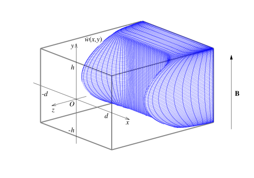
Figure 1: The base flow profile in a square duct with thin conducting walls subject to a vertical magnetic field for $c=0.1$ and $\mathit{Ha}=100.$

2 Formulation of the problem

Consider the flow of an incompressible viscous electrically conducting liquid with density $\rho,$ kinematic viscosity $\nu$ and electrical conductivity $\sigma$ driven by a constant gradient of pressure $p$ applied along the axis of straight duct of rectangular cross-section with half-width $d$ and half-height $h$ subject to a transverse homogeneous magnetic field $\mbox{\boldmath$\mathit{B}$}.$ The walls of the duct are assumed to have small thickness $d_{w}\ll d$ and electrical conductivity $\sigma_{w}.$

The liquid flow is governed by the Navier-Stokes equation

$$\partial_{t}\mbox{\boldmath$\mathit{v}$}+(\mbox{\boldmath$\mathit{v}$}\cdot\mbox{\boldmath$\mathit{\nabla}$})\mbox{\boldmath$\mathit{v}$}=-\rho^{-1}\mbox{\boldmath$\mathit{\nabla}$}p+\nu\mbox{\boldmath$\mathit{\nabla}$}^{2}\mbox{\boldmath$\mathit{v}$}+\rho^{-1}\mbox{\boldmath$\mathit{f}$},$$ (1)

with the electromagnetic body force $\mbox{\boldmath$\mathit{f}$}=\mbox{\boldmath$\mathit{j}$}\times\mbox{\boldmath$\mathit{B}$}$ involving the induced electric current $\mbox{\boldmath$\mathit{j}$},$ which is governed by Ohm’s law for a moving medium,

$$\mbox{\boldmath$\mathit{j}$}=\sigma(\mbox{\boldmath$\mathit{E}$}+\mbox{\boldmath$\mathit{v}$}\times\mbox{\boldmath$\mathit{B}$}).$$ (2)

The flow is assumed to be sufficiently slow for the induced magnetic field to be negligible relative to the imposed one. This corresponds to the so-called inductionless approximation, which holds for small magnetic Reynolds numbers $\mathit{Rm}=\mu_{0}\sigma v_{0}d\ll 1,$ where $\mu_{0}$ is the permeability of free space and $v_{0}$ is a characteristic velocity of the flow. In addition, we assume the characteristic time of velocity variation to be much longer than the magnetic diffusion time $\tau_{m}=\mu_{0}\sigma d^{2}.$ This is known in MHD as the quasi-stationary approximation (Roberts, 1967), which leads to $\mbox{\boldmath$\mathit{E}$}=-\mbox{\boldmath$\mathit{\nabla}$}\phi,$ where $\phi$ is the electrostatic potential. The velocity and current satisfy mass and charge conservation, $\mbox{\boldmath$\mathit{\nabla}$}\cdot\mbox{\boldmath$\mathit{v}$}=0,\mbox{\boldmath$\mathit{\nabla}$}\cdot\mbox{\boldmath$\mathit{j}$}=0.$ Applying the latter to Ohm’s law (2) and using the inductionless approximation, we obtain

$$\mbox{\boldmath$\mathit{\nabla}$}^{2}\phi=\mbox{\boldmath$\mathit{B}$}\cdot\mbox{\boldmath$\mathit{\omega}$},$$ (3)

where $\mbox{\boldmath$\mathit{\omega}$}=\mbox{\boldmath$\mathit{\nabla}$}\times\mbox{\boldmath$\mathit{v}$}$ is the vorticity. At the duct walls $S$, the normal $(n)$ and tangential $(\tau)$ velocity components satisfy the impermeability and no-slip boundary conditions $\left.v_{n}\right|_{s}=0$ and $\left.v_{\tau}\right|_{s}=0.$ Charge conservation applied to the thin wall leads to the following boundary condition, $\left.\partial_{n}\phi-dc\mbox{\boldmath$\mathit{\nabla}$}_{\tau}^{2}\phi\right|_{s}=0,$ where $c=\sigma_{w}d_{w}/(\sigma d)$ is the wall conductance ratio (Walker, 1981). At the corner point $P$, this condition reduces to that of the continuity of the tangential current in the wall, i.e. $\left[dc\partial_{\tau}\phi\right]_{P}=0,$ where the square brackets denote the jump in the enclosed quantity.

We employ Cartesian coordinates, with the origin set at the centre of the duct, $x$-, $y$- and $z$-axes directed along its width, height and length, respectively, as shown in figure 1, and the velocity defined as $\mbox{\boldmath$\mathit{v}$}=(u,v,w).$ The problem admits a purely rectilinear base flow with a single velocity component along the duct $\bar{\mbox{\boldmath$\mathit{v}$}}=(0,0,\bar{w}(x,y)),$ which is shown in figure 1 for $c=0.1$ and $\mathit{Ha}=100.$

In the following, all variables are non-dimensionalized by using the maximum velocity $\bar{w}_{0}$ and the half-width of the duct $d$ as the velocity and length scales. The time, pressure, magnetic field and electrostatic potential are scaled by $d^{2}/\nu,$ $\rho\bar{w}_{0}^{2},$ $B=\left|\mbox{\boldmath$\mathit{B}$}\right|$ and $\bar{w}_{0}dB,$ respectively. Note that we use the maximum rather than average velocity of the base flow as the characteristic scale because the stability of this flow is determined by the former.

The base flow can conveniently be determined using the $z$-component of the induced magnetic field $\bar{b}$ instead of the electrostatic potential $\bar{\phi}.$ Then the governing equations for the base flow take the form

$$\mbox{\boldmath$\mathit{\nabla}$}^{2}\bar{w}+\mathit{Ha}\partial_{y}\bar{b} = \bar{P,}$$ (4)

$$\mbox{\boldmath$\mathit{\nabla}$}^{2}\bar{b}+\mathit{Ha}\partial_{y}\bar{w} = 0,$$ (5)

where $\mathit{Ha}=dB\sqrt{\sigma/(\rho\nu)}$ is the Hartmann number and $\bar{b}$ is scaled by $\mu_{0}\sqrt{\sigma\rho\nu^{3}}/d.$ The constant dimensionless axial pressure gradient $\bar{P}$ that drives the flow is determined from the normalization condition $\bar{w}_{\max}=1.$ The velocity satisfies the no-slip boundary condition $\bar{w}=0$ at $x=\pm 1$ and $y=\pm A,$ where $A=h/d$ is the aspect ratio, which is set equal to $1$ for the square cross-section duct considered in this study. The boundary condition for the induced magnetic field at the thin wall is

$$\bar{b}=c\partial_{n}\bar{b}.$$ (6)

The linear stability of the flow is analysed using a non-standard vector streamfunction-vorticity formulation (Priede et al., 2010, 2012). Following this approach, a vector streamfunction $\mathit{\psi}$ is introduced to satisfy the incompressibility constraint $\mbox{\boldmath$\mathit{\nabla}$}\cdot\mbox{\boldmath$\mathit{v}$}=0$ for the flow perturbation by seeking the velocity distribution in the form $\mbox{\boldmath$\mathit{v}$}=\mbox{\boldmath$\mathit{\nabla}$}\times\mbox{\boldmath$\mathit{\psi}$}.$ Each component of $\mathit{\psi}$ describes a solenoidal flow with two velocity components in the plane transverse to that component where the isolines of the respective component of $\mathit{\psi}$ represent the streamlines of that flow. Since $\mathit{\psi}$ is determined up to a gradient of arbitrary function, an additional constraint

$$\mbox{\boldmath$\mathit{\nabla}$}\cdot\mbox{\boldmath$\mathit{\psi}$}=0,$$ (7)

which is analogous to the Coulomb gauge for the magnetic vector potential $\mathit{A}$ (Jackson, 1998), can be applied. Similar to the incompressibility constraint for $\mbox{\boldmath$\mathit{v}$},$ this gauge leaves only two independent components of $\mbox{\boldmath$\mathit{\psi}$}.$

The pressure gradient is eliminated by taking the curl of the dimensionless counterpart of (1), which leads to the following equations for $\mathit{\psi}$ and $\mathit{\omega}$:

$$\partial_{t}\mbox{\boldmath$\mathit{\omega}$} = \mbox{\boldmath$\mathit{\nabla}$}^{2}\mbox{\boldmath$\mathit{\omega}$}-\mathit{Re}\mbox{\boldmath$\mathit{g}$}+\mathit{Ha}^{2}\mbox{\boldmath$\mathit{h}$},$$ (8)

$$0 = \mbox{\boldmath$\mathit{\nabla}$}^{2}\mbox{\boldmath$\mathit{\psi}$}+\mbox{\boldmath$\mathit{\omega}$},$$ (9)

where $\mathit{Re}=\bar{w}_{0}d/\nu$ is the Reynolds number based on the maximum jet velocity $\bar{w}_{0}$,and $\mbox{\boldmath$\mathit{g}$}=\mbox{\boldmath$\mathit{\nabla}$}\times(\mbox{\boldmath$\mathit{v}$}\cdot\mbox{\boldmath$\mathit{\nabla}$})\mbox{\boldmath$\mathit{v}$},$ and $\mbox{\boldmath$\mathit{h}$}=\mbox{\boldmath$\mathit{\nabla}$}\times\mbox{\boldmath$\mathit{f}$}$ are the curls of the dimensionless convective inertial and electromagnetic forces, respectively.

The boundary conditions for $\mathit{\psi}$ and $\mathit{\omega}$ are derived as follows. The impermeability condition applied integrally as $\int_{s}\mbox{\boldmath$\mathit{v}$}\cdot\mbox{\boldmath$\mathit{\mathrm{d}s}$}=\oint_{l}\mbox{\boldmath$\mathit{\psi}$}\cdot\mbox{\boldmath$\mathit{\mathrm{d}l}$}=0$ to an arbitrary area of wall $s$ encircled by a contour $l$ yields $\left.\psi_{\tau}\right|_{s}=0.$ This boundary condition substituted into (7) results in $\left.\partial_{n}\psi_{n}\right|_{s}=0.$ In addition, the no-slip condition applied integrally, $\oint_{l}\mbox{\boldmath$\mathit{v}$}\cdot\mbox{\boldmath$\mathit{\mathrm{d}l}$}=\int_{s}\mbox{\boldmath$\mathit{\omega}$}\cdot\mbox{\boldmath$\mathit{\mathrm{d}s}$}$, yields $\left.\omega_{n}\right|_{s}=0.$

The linear stability of the base flow $\{\bar{\mbox{\boldmath$\mathit{\psi}$}},\bar{\mbox{\boldmath$\mathit{\omega}$}},\bar{\phi}\}(x,y)$ is analysed with respect to infinitesimal disturbances in the standard form of harmonic waves travelling along the axis of the duct,

$$\{\mbox{\boldmath$\mathit{\psi}$},\mbox{\boldmath$\mathit{\omega}$},\phi\}(\mbox{\boldmath$\mathit{r}$},t)=\{\bar{\mbox{\boldmath$\mathit{\psi}$}},\bar{\mbox{\boldmath$\mathit{\omega}$}},\bar{\phi}\}(x,y)+\{\hat{\mbox{\boldmath$\mathit{\psi}$}},\hat{\mbox{\boldmath$\mathit{\omega}$}},\hat{\phi}\}(x,y)e^{\lambda t+\mathrm{i}kz},$$

where $k$ is a real wavenumber and $\lambda$ is, in general, a complex growth rate. This expression substituted into (8,9) results in

$$\lambda\hat{\mbox{\boldmath$\mathit{\omega}$}} = \mbox{\boldmath$\mathit{\nabla}$}_{k}^{2}\hat{\mbox{\boldmath$\mathit{\omega}$}}-\mathit{Re}\hat{\mbox{\boldmath$\mathit{g}$}}+\mathit{Ha}^{2}\hat{\mbox{\boldmath$\mathit{h}$}},$$ (10)

$$0 = \mbox{\boldmath$\mathit{\nabla}$}_{k}^{2}\hat{\mbox{\boldmath$\mathit{\psi}$}}+\hat{\mbox{\boldmath$\mathit{\omega}$}},$$ (11)

$$0 = \mbox{\boldmath$\mathit{\nabla}$}_{k}^{2}\hat{\phi}-\hat{\omega}_{\shortparallel},$$ (12)

where and$\shortparallel$ and $\perp$ respectively denote the components along and transverse to the magnetic field in the $(x,y)$-plane. Because of the solenoidality of $\hat{\mbox{\boldmath$\mathit{\omega}$}},$ it suffices to consider only the $x$- and $y$-components of (10), which contain $\hat{h}_{\perp}=-\partial_{xy}\hat{\phi}-\partial_{\shortparallel}\hat{w},$ $\hat{h}_{\shortparallel}=-\partial_{\shortparallel}^{2}\hat{\phi}$ and

$$\hat{g}_{x} = k^{2}\hat{v}\bar{w}+\partial_{yy}(\hat{v}\bar{w})+\partial_{xy}(\hat{u}\bar{w})+\mathrm{i}2k\partial_{y}(\hat{w}\bar{w}),$$ (13)

$$\hat{g}_{y} = -k^{2}\hat{u}\bar{w}-\partial_{xx}(\hat{u}\bar{w})-\partial_{xy}(\hat{v}\bar{w})-\mathrm{i}2k\partial_{x}(\hat{w}\bar{w}),$$ (14)

where

$$\hat{u} = \mathrm{i}k^{-1}(\partial_{yy}\hat{\psi}_{y}-k^{2}\hat{\psi}_{y}+\partial_{xy}\hat{\psi}_{x}),$$ (15)

$$\hat{v} = -\mathrm{i}k^{-1}(\partial_{xx}\hat{\psi}_{x}-k^{2}\hat{\psi}_{x}+\partial_{xy}\hat{\psi}_{y}),$$ (16)

$$\hat{w} = \partial_{x}\hat{\psi}_{y}-\partial_{y}\hat{\psi}_{x}.$$ (17)

The relevant boundary conditions are

$$\partial_{x}^{2}\hat{\phi}-k^{2}\hat{\phi}-c^{-1}\partial_{y}\hat{\phi}=\hat{\psi}_{y}=\partial_{x}\hat{\psi}_{x}=\partial_{x}\hat{\psi}_{y}-\partial_{y}\hat{\psi}_{x}=\hat{\omega}_{x}=0 x=\pm 1,$$ at (18)

$$\partial_{y}^{2}\hat{\phi}-k^{2}\hat{\phi}-c^{-1}\partial_{x}\hat{\phi}=\hat{\psi}_{x}=\partial_{y}\hat{\psi}_{y}=\partial_{x}\hat{\psi}_{y}-\partial_{y}\hat{\psi}_{x}=\hat{\omega}_{y}=0 y=\pm A.$$ at (19)

3 Numerical procedure

The problem was solved by a spectral collocation method on a Chebyshev-Lobatto grid with even number of points $2N_{x}+2$ and $2N_{y}+2$ in the $x$- and $y$-directions, where $N_{x,y}=35\cdots 70$ were used for various combinations of the control parameters to achieve accuracy of at least three significant figures. Accuracy was verified by recalculating dubious results with a higher numerical resolution using typically five more collocation points in each direction. The number of collocation points required for a sufficiently accurate solution was found to increase with the Hartmann number reaching $N_{x,y}=70$ at $\mathit{Ha}=10^{4}.$ Owing to the double reflection symmetry of the base flow with respect to the $x=0$ and $y=0$ planes, small-amplitude perturbations with different parities in $x$ and $y$ decouple from each other. This results in four mutually independent modes, which we classify as $(o,o),$ $(o,e),$ and $(e,e)$ according to whether the $x$ and $y$ symmetry of $\hat{\psi}_{x}$ is odd or even, respectively. Our classification of modes corresponds to the symmetries I, II, III and IV used by Tatsumi & Yoshimura (1990) and Uhlmann & Nagata (2006) (see table 1). The symmetry allows us to solve the linear stability problem for each of the four modes separately using only one quadrant of the duct cross-section with $N_{x}\times N_{y}$ internal collocation points.

The four modes listed in table 1 have the following spatial structure. Mode I has a $y$-component of streamfunction-vorticity that which is even in both the $x$- and $y-$directions, i.e. mirror-symmetric with respect to both mid-planes. This corresponds to vertical vortices that rotate in the same sense in all four quadrants of the duct. Such vortices can span the height of the duct and thus, can be relatively uniform along a vertical magnetic field. It also means that the vortices at the opposite sidewalls rotate in the same sense and thus can enhance each other through a shared flux across the vertical mid-plane of the duct. Mode II differs from mode I by the opposite vertical symmetry. It means that the vertical vortices associated with this mode change their direction of rotation at the horizontal mid-plane and rotate in the opposite senses in the top and bottom parts of the duct. Such vortices are inherently non-uniform along the height of the duct and thus subject to a strong damping by the vertical magnetic field. Modes III and IV differ from modes I and II by the opposite spanwise symmetry. It means that the vertical vortices at the opposite sidewalls for these two modes rotate in the opposite senses and are separated from each other by the vertical mid-plane of the duct. The symmetry of the $x$-component of streamfunction-vorticity, which is associated with spanwise vortices, is always opposite to that of the $y$-component. This follows from the symmetry of the associated velocity components, which are defined in terms of $\hat{\psi}_{x}$ and $\hat{\psi}_{y}$ by (15-17). Note that modes I and IV differ from one another only by a $90^{\circ}$ rotation around the $z$-axis, which is not the case for modes II and III.

	I	II	III	IV
$\hat{\psi}_{x},\,\hat{\omega}_{x},\,\hat{v}:$	$(o,o)$	$(o,e)$	$(e,o)$	$(e,e)$
$\hat{w}:$	$(o,e)$	$(o,o)$	$(e,e)$	$(e,o)$
$\hat{\psi}_{z},\,\hat{\omega}_{z}:$	$(e,o)$	$(e,e)$	$(o,o)$	$(o,e)$
$\hat{\psi}_{y},\,\hat{\omega}_{y},\,\hat{u},\,\phi:$	$(e,e)$	$(e,o)$	$(o,e)$	$(o,o)$

Table 1: The $(x,y)$ parities of different variables for symmetries I, II, III and IV; $e$ - even, $o$ - odd

The numerical procedure employed in this study is basically the same as that used by Priede et al. (2010), where a detailed description and validation of the code are presented. The only major difference is that the original code was designed for perfectly electrically conducting and insulating walls, whereas here walls with a finite electrical conductivity are considered. This leads to different boundary conditions for both the induced magnetic field (6) and the electric potential (18), (19). Owing to the fact that the Laplace operator on the l.h.s of (12) turns into the electric boundary condition when the second-order partial derivative normal to the boundary is substituted by the respective first-order derivative divided by negative wall conductivity ratio as in (18) and (19), the electric potential can efficiently be eliminated from the problem by using the matrix diagonalization algorithm (Canuto et al., 2007, Sec. 4.1.4) to invert the discretized counterpart of (12).

4 Results

4.1 Base flow

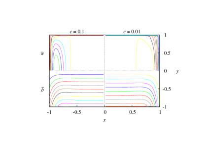
Figure 2: (a) Isolines of the base flow velocity $(y>0)$ and the electric current lines $(y<0)$ for $c=0.1$ $(x<0)$ and $c=0.01$ $(x>0)$ at $\mathit{Ha}=100$ shown in the respective quadrants of the duct cross-section; and (b)the horizontal base flow velocity profiles in the vicinity of the side-wall at $y=0$ in stretched coordinate $(1-x)\mathit{Ha}^{1/2}$ for various Hartmann numbers and $c=0.1.$

Let us first consider the characteristics of the base flow that are pertinent to its stability. The most prominent feature of the base flow is the high-velocity jets that form in the strong magnetic field along the sidewalls of the duct provided that the conductance ratio is sufficiently high for the given magnetic field strength. This effect is illustrated by figures 1 and 2(a), where the jets are seen to be pronounced at $\mathit{Ha}=100$ and $c=0.1$ and then to become relatively weak at the wall conductance ratio $c=0.01.$ The velocity of the jets relative to that of the core flow typically increases as $\sim\mathit{Ha}^{1/2}$ while their thickness reduces as $\sim\mathit{Ha}^{-1/2}.$ As seen in figure 2(b), the velocity maximum

$$\bar{w}_{\max}\sim-0.2825c^{-1}\mathit{Ha}^{-3/2}\bar{P},$$ (20)

which follows from the asymptotic solution (31) presented in the appendix A, is located at distance $\delta\sim 0.92\mathit{Ha}^{-1/2}$ from the sidewall. The velocity in the core of the flow defined by (30) is $\bar{w}_{\textrm{core}}\sim-(1+c^{-1})\mathit{Ha}^{-2}\bar{P}.$ Thus, the fraction of the volume flux carried by the jets is comparable to that carried by the core flow. In a strong magnetic field, this fraction is expected to approach a constant determined solely by $c.$ As seen in figure 3(a), an extremely strong magnetic field is required to achieve this asymptotic flow regime. For example, the volume flux fraction carried by the the sidewall jets for $c=0.01$ at $\mathit{Ha}=10^{6}$ is still approximately $8\%$ below its asymptotic value $\gamma=\frac{1}{4.03},$ which follows from (39). For a fixed $\mathit{Ha},$ $\gamma$ is seen in figure 3(b) to attain a maximum at $c\approx\mathit{Ha}^{-1/4}$ in a good agreement with the asymptotic solution (41). It is important to note that, at this point, $\gamma$ starts to deviate from its asymptotic value for $\textit{Ha}\rightarrow\infty$ when $c$ is reduced. Thus, for $\gamma$ to reach its high-field asymptotic limit (40) at $c\ll 1,$ an extremely strong magnetic field with $\mathit{Ha}\sim c^{-4}$ is required. For the base flow normalized with the maximal velocity, which is used as the characteristic velocity in this study, the total volume flux is seen in figure 3(c) to approach the value predicted by the asymptotic solution,

$$Q\sim\left(\tfrac{4}{3}+c\right)/(0.2825\mathit{Ha}^{1/2}),$$ (21)

where the normalization coefficient at $\mathit{Ha}^{1/2}$ follows from (20). This relation can be used to rescale our results with the average velocity in a sufficiently strong magnetic field. We use an overbar to distinguish the Reynolds number based on the total volume flux from that introduced earlier using the maximal jet velocity.

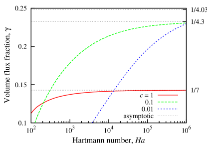
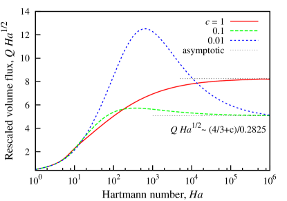
Figure 3: The volume flux fraction $\gamma$ carried by the side-wall jets (a) depending on the Hartmann number for fixed wall conductance ratios $c=1,0.1,0.01,$ and (b) versus the wall conductance ratio for various Hartmann numbers with the asymptotic solution (38) shown by the thin dotted lines; (c) rescaled total volume flux $Q\mathit{Ha}^{1/2}$ versus the Hartmann number for the base flow normalized with maximal jet velocity with the asymptotic solution (21) shown by the thin dotted lines.

4.2 Linear stability

The following results are for the flow in a square duct $(A=1)$, which is linearly stable without the magnetic field (Tatsumi & Yoshimura, 1990). We start with a moderate wall conductance ratio $c=1$ at which the flow is expected to be similar to that in a perfectly conducting duct. As in the perfectly conducting duct (Priede et al., 2012), the magnetic field renders the flow linearly unstable at $\mathit{Ha}\gtrsim 10$ with respect to a mode of symmetry type II (see table 1). The vorticity component along the magnetic field of this mode is an odd function in the field direction and an even function spanwise. The marginal Reynolds number, at which the growth rate turns to zero $(\Re[\lambda]=0),$ and the associated relative phase speed $-\omega/(\mathit{Re}k)$, which is defined by the imaginary part of the growth rate $\omega=\Im[\lambda]$ relative to the maximum jet velocity $\mathit{Re}$, are plotted against the wavenumber in figure 4. The lowest point on each marginal Reynolds number curve defines a critical Reynolds number $\mathit{Re}_{c}$ at which the flow first becomes unstable at the given Hartmann number. These points are marked by dots in figure 4 and also plotted in figure 6 against the Hartmann number. In figure 6, the mode II instability is seen to appear at $\mathit{Ha}\approx 10$ and very high $\mathit{Re}_{c}.$ With increase of the Hartmann number, $\mathit{Re}_{c}$ quickly drops to the minimum $\mathit{Re}_{c}\approx 6500$ at $\mathit{Ha}\approx 13$ and then starts to increase, reaching $\mathit{Re}_{c}\approx 6\times 10^{4}$ at $\mathit{Ha}=100.$ The steep stabilization of this mode is due to its antisymmetric vorticity distribution along the magnetic field, which is smoothed out and thus efficiently suppressed by the magnetic field.

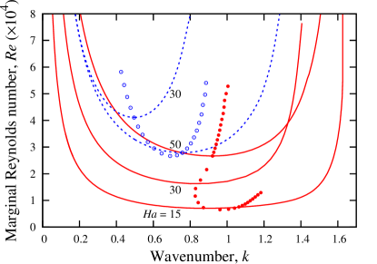
Figure 4: The marginal Reynolds number (a) and the relative phase velocity (b) versus the wavenumber for neutrally stable modes of type II and IV in a square duct $(A=1)$ with the wall conductance ratio $c=1$ at various Hartmann numbers which are shown next to the curves. Dots indicate the critical points, which correspond to the lowest marginal $\mathit{Re}$ for each $\mathit{Ha};$ these points cover a broader range of $\mathit{Ha}$ than the marginal stability curves.

A similar instability mode, which is of type IV and differs from mode II by the opposite spanwise symmetry, appears at $\mathit{Ha}\approx 28.$ Although this mode becomes more unstable than mode II at $\mathit{Ha}\gtrsim 55,$ both modes are superseded by a more unstable mode of symmetry I, which emerges at $\mathit{Ha}\approx 27$ and becomes dominating at $\mathit{Ha}\gtrsim 29.$ In contrast to modes II and IV, the vorticity component along the magnetic field of mode I is an even function in the field direction. Marginal Reynolds number and the relative phase velocity for this mode iare shown in figure 5. The last instability mode for $c=1,$ which appears at $\mathit{Ha}\approx 37,$ is of type III, and it differs from mode I by the opposite spanwise symmetry. Although the critical Reynolds number for mode III is initially significantly higher than that for mode I, with increase of the Hartmann number the difference between the two modes quickly diminishes and becomes negligible at $\mathit{Ha}\gtrsim 100$ (see figure 6). This is due to the localization of unstable perturbations at the sidewalls, which takes place in a sufficiently strong magnetic field when a virtually stagnant core of the flow forms. Also note that the increase of the critical Reynolds number with the Hartmann number for modes I/III is much slower than that for modes II/IV. This is due to the even distribution of the vorticity component along the magnetic field which makes modes I/III less susceptible to the magnetic field than modes II/IV.

For lower wall conductance ratios $c=0.1,0.01,$ instability is seen in figure 6 to emerge at larger Hartmann numbers. As discussed below, this is because the finite conductivity of the walls normal to the magnetic field becomes important at $\mathit{Ha}\gtrsim c^{-1}.$

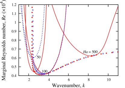
Figure 5: The marginal Reynolds number (a) and the relative phase velocity (b) versus the wavenumber for neutrally stable modes of type I and III in a square duct $(A=1)$ with the wall conductance ratio $c=1$ at various Hartmann numbers.

The critical Reynolds number for modes I/III can be seen in figure 6(a) to increase asymptotically as $\mathit{Re}_{c}\sim\mathit{Ha}^{1/2}.$ This asymptotic regime requires a relatively strong magnetic field, especially for low wall conductance ratio. Namely, for $c=0.01,$ asymptotics start to emerge at $\mathit{Ha}\gtrsim 10^{4}.$ The best fit including the two subsequent terms, which are significant for $\mathit{Ha}\gtrsim 10^{3}$ and according to the asymptotic solution (37) are $O(\mathit{Ha}^{-1/2})$ and $O(\mathit{Ha}^{-1})$ relative to the leading-order term, gives $\mathit{Re}_{c}\sim\kappa\mathit{Ha}^{1/2}$ with $\kappa\approx 109\pm 1.5$ for $c=1,0.1$ and $\kappa\approx 120\pm 10$ for $c=0.01.$ These asymptotics imply that the relevant length scale for the instability modes I/III is the thickness of the side layers $\delta\sim\mathit{Ha}^{-1/2}.$ This is confirmed by the critical wavenumber, which is seen in figure 6(b) to increase asymptotically as $k_{c}\sim 0.5\mathit{Ha}^{1/2}$ for all wall conductance ratios. Since the frequency based on this length scale is expected to scale as $\omega\sim\mathit{Ha},$ the relative phase velocity for modes I/III, which is plotted in figure 6(c), approaches a constant at a sufficiently large Hartmann number. The best fit including the three leading terms yields $-\omega/(\mathit{Re}k)\approx 0.47$ for $c=1,0.1$ and $-\omega/(\mathit{Re}k)\approx 0.48$ for $c=0.01.$ This means that the unstable modes I/III travel downstream with nearly half of the maximal jet velocity. The phase velocity for modes II/IV is seen in figure 6(c) to be noticeably higher and approaches $0.8$ at $\mathit{Ha}\approx 100.$

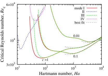
Figure 6: The critical Reynolds number (a), wavenumber (b) and relative phase velocity (c) against the Hartmann number for wall conductance ratios $c=1,$ 0.1, 0.01. Modes II and IV are shown only for $c=1.$

Variation of the critical Reynolds number and the associated wavenumber with the wall conductance ratio is shown in figure 7. As the wall conductance ratio $c$ reduces, the flow is seen to become linearly very stable as in the duct with insulating walls. The higher the Hartmann number, the smaller is the wall conductance ratio down to which the instability persists. This is because the effect of $c$ is determined by the relative conductance of the Hartmann layer, which drops directly with its thickness as $\sim\mathit{Ha}^{-1}.$ Thus, for $c\ll 1$ and $\mathit{Ha}\gg 1,$ the relevant parameter is $c\mathit{Ha}$ which according to (26) has to be sufficiently small for the wall to be effectively insulating. Figure 7(a) indicates that the flow becomes linearly stable when $c\mathit{Ha}\lesssim 1.$ However, the stabilization of the flow does not proceed monotonically with the reduction of the wall conductance ratio. For sufficiently large Hartmann numbers $(\mathit{Ha}\gtrsim 500),$ the critical Reynolds number is seen in figure 7(a) first to drop slightly before eventually starting to rise when the wall conductance ratio approaches $c\sim\mathit{Ha}^{-1}.$ This weak destabilization of the flow is associated with the development of the sidewall jets, which according to (41) attain maximum fraction of the volume flux at $c\approx\mathit{Ha}^{-1/4}$ (see figure 3b). Thus, the lowest critical Reynolds numbers for $\mathit{Ha}=500$ and $1000$ occur at $c\approx 0.2$ and $0.18,$ respectively. Owing to this slight minimum, the overall variation of $\mathit{Re}_{c}$ at high Hartmann numbers remains relatively weak down to $c\sim 10^{-2}.$

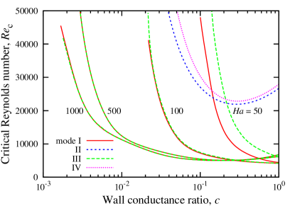
Figure 7: The critical Reynolds number (a) and the wavenumber (b) versus the wall conductance ratio at various Hartmann numbers.

The complex amplitude distribution of the critical mode I streamwise velocity perturbation $\hat{w}$ $(x<0)$ and the same streamfunction component $\hat{\psi}_{z}$ $(x>0),$ which both are mirror-symmetric with respect to the vertical mid-plane $x=0,$ are shown in figure 8(a) for $c=0.1$ and $\mathit{Ha}=10^{3}.$ These two quantities define respectively the potential and solenoidal components of the flow perturbation in the cross-section of the duct. At this high Hartmann number, the perturbations are seen to be localized at the sidewalls and effectively separated by a virtually unperturbed fluid core. This makes the perturbation pattern for mode I practically indistinguishable from that for mode III, which differs from the former only by the opposite $x$ symmetry.

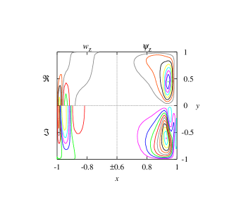
Figure 8: Amplitude distributions of the real $(y>0)$ and imaginary $(y<0)$ parts of $\hat{w}$ $(x<0)$ and $\hat{\psi}_{z}$ $(x>0)$ (a) and the isosurfaces of $\hat{\psi}_{y}$ of the critical perturbation of mode I in the vicinity of side-wall over half height of duct cross-section for $\mathit{Ha}=10^{3}$ the wall conductance ratio $c=0.1.$

The real and imaginary parts, which are plotted in the upper $(y>0)$ and lower $(y<0)$ halves of the duct, are defined by the normalization condition $\int_{S}\Re[\mbox{\boldmath$\mathit{\hat{v}]}$}^{2}\,\mathrm{d}s=\int_{S}\Im[\mbox{\boldmath$\mathit{\hat{v}]}$}^{2}\,\mathrm{d}s,$ where the integrals are taken over the duct cross-section $S.$ The latter two quantities define perturbation distributions over the duct cross-section shifted in time or in the streamwise direction by a quarter of a period or wavelength, respectively. The isolines of $\hat{\psi}_{z}$ show the streamlines of the rotational flow perturbation component in the cross-sectional plane. Circulation for mode I is seen to be dominated by one vortex that stretches along the sidewall in each quadrant of the duct. This vortex advects the non-uniformly distributed momentum in the sidewall jets, so giving rise to the streamwise velocity perturbation $\hat{w}$ which is shown on the left-hand side of figure 8(a). Since the latter varies streamwise, it gives rise to a converging flow perturbation over tthe cross-section where the base flow is accelerated and to a diverging one where the base flow is slowed down. This, in turn, gives rise to a circulation in the plane transverse to the magnetic field, i.e. in the $xz$-plane, which is defined by $\psi_{y}.$ The spatial pattern of this quantity is shown in figure 8(b) over the wavelength for one quadrant of the duct. The lines of constant $\psi_{y}$ correspond to the streamlines of flow perturbation in the $xz$-plane. Note that the spatial distribution of $\psi_{y}$ is very similar to that of the electric potential perturbation $\phi.$ This is because both quantities are governed by identical equations (11,12), and differ only by the boundary conditions (18,19). As seen in figure 9(a,b), the isolines of $\psi_{y}$ $(x>0)$ and $\phi$ $(x<0)$ are nearly identical in the horizontal mid-plane $(y=0)$, whereas they differ more from each other at thehorizontal walls $(y=\pm 1).$ Analogous distributions of $\psi_{x}$ $(y>0)$ and $\phi$ $(y<0)$ at the sidewalls $(x=\pm 1)$ of the duct can be seen in figure 9(c). Note that the apparent flow implied by the streamlines at the solid walls, where according to the no-slip condition flow must be absent, are due to the streamfunction decomposition. In contrast to the velocity components, which satisfy the boundary conditions separately and the solenoidality condition all together, each streamfunction component defines a solenoidal velocity field that satisfies only the impermeability condition whereas the no-slip condition is satisfied by all streamfunction components together.

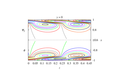
Figure 9: Isolines of $\psi_{y}$ $(x>0)$ and $\phi$ $(x<0)$ in the mid-plane $(y=0)$ (a) and at the horizontal walls $(y=\pm 1)$ (b); isolines of $\psi_{x}$ $(y>0)$ and $\phi$ $(y<0)$ at the side walls $(x=\pm 1)$ of the duct for the critical perturbation of mode I at $\mathit{Ha}=10^{3}$ and $c=0.1.$ The isoline spacing in (b) as well as that for $\psi_{x}$ in (c) is by a factor of $10$ smaller, whereas for $\phi$ in (c) it is by a factor $100$ smaller than the original spacing in (a).

The component of the flow perturbation associated with the vorticity along the magnetic field, which is shown in figure 8(b), dominates the instability in a sufficiently strong magnetic field. Namely, for -$\mathit{Ha}=10^{3}$ and the wall conductance ratios $c$ from $1$ to $0.01,$ the $y$-component of vorticity-stream function carries $99\%$ to $97\%$ of the perturbation energy,

$$E\propto\int_{S}\hat{\left|\mbox{\boldmath$\mathit{v}$}\right|}^{2}\,\mathrm{d}s=\int_{S}\Re[\hat{\mbox{\boldmath$\mathit{\omega}$}}\cdot\hat{\mbox{\boldmath$\mathit{\psi}$}}^{*}]\,\mathrm{d}s,$$

whereas the $y$-component of the velocity perturbation carries respectively $1\%$ to $3\%$ of $E.$ This suggests that the flow perturbation in a high magnetic field is dominated by a single streamfunction-vorticity component aligned with the magnetic field.

5 Summary and conclusions

We have presented analytical and numerical results concerning MHD flow and its linear stability in a square duct with thin conducting walls. First, we extended the original asymptotic solution obtained by Walker (1981) for the base flow in a high magnetic field to moderate magnetic fields. The asymptotic solution, which was confirmed by the numerical results, showed that the fraction of the volume flux carried by the side layers attains its maximum at the wall conductance ratio $c\sim\mathit{Ha}^{-1/4}.$ For $c\ll 1,$ this implies that an extremely strong magnetic field with $\mathit{Ha}\sim c^{-4}$ is required for the sidewall jets to fully develop.

In a square duct with moderate wall conductance ratio $c=1,$ the flow was found to become linearly unstable at $\mathit{Ha}\gtrsim 10.$ The vorticity component along the magnetic field for the first instability mode is an odd function in the field direction and an even function in the spanwise direction. There is another slightly more stable mode that differs from the previous one by the opposite spanwise symmetry. The increase of the magnetic field, which smooths out the flow perturbation along the flux lines, results in a strong damping of these two instability modes. In a strong magnetic field, the instability is dominated by two additional modes which differ from the previous two by the even vorticity distribution along the magnetic field. This makes the latter two modes more uniform along the magnetic field and thus less susceptible to damping. The spanwise symmetric mode is slightly more unstable than the antisymmetric mode. This is because the former consists of the vortices at the opposite sidewalls which are co-rotating and thus enhancing each other through a shared flux, whereas the contrary is the case for the latter mode. This difference becomes insignificant in a strong magnetic field, where the opposite vortices are effectively separated by a virtually unperturbed core flow. In this case, the critical Reynolds number based on the jet velocity and the associated wavenumber for both modes increase asymptotically as $\mathit{Re}_{c}\sim 110\mathit{Ha}^{1/2}$ and $k_{c}\sim 0.5\mathit{Ha}^{1/2},$ while the modes travel downstream with a phase speed close to half of maximal jet velocity. These asymptotics imply that the instability takes place in the sidewall jets with the characteristic thickness $\delta\sim\mathit{Ha}^{-1/2}$ which determines the actual length scale of the instability.

When the magnetic field is sufficiently strong, the reduction of the wall conductance ratio results in a weak destabilization of the flow until $c\sim\mathit{Ha}^{-1/4},$ where the critical Reynolds number attains a minimum and then starts to increase as $c$ is reduced further. This slight minimum of $\mathit{Re}_{c}$ corresponds to the wall conductance ratio discussed above at which the fraction of the volume flux carried by the sidewall jets attains a maximum. The critical Reynolds number becomes very high at $c\lesssim\mathit{Ha}^{-1},$ which corresponds to the wall conductance ratio smaller than that of the Hartmann layer. At this point, the walls become effectively insulating, which leads to the transformation of the sidewall jets into the Shercliff layers (Shercliff, 1953) The latter are expected to become linearly unstable like the Hartmann layer at $\mathit{Re}_{c}\sim 10^{4}\mathit{Ha}^{1/2}$ (Pothérat, 2007), which is too high to be reliably computed using the current numerical method. It may also be of little significance as the flow in the insulating duct is known to be turbulent at much lower Reynolds numbers (Shatrov & Gerbeth, 2010).

This, however, is not necessarily the case for the flows with sidewall jets, which have relatively low critical Reynolds numbers. Namely, the critical Reynolds number $\mathit{Re}_{c}\sim 91\mathit{Ha}^{1/2}$ for Hunt’s flow, which has jets very similar to those in the duct with thin walls, is a bit lower than that found in this study. Both flows also have very close critical wavenumbers and phase speeds. In contrast, the flow in a perfectly conducting duct, which has much weaker jets, has a critical Reynolds number $\mathit{Re}_{c}\sim 642\mathit{Ha}^{1/2},$ which is significantly higher than that for the two other flows. Finally, rescaling our critical Reynolds number with the total volume flux (21) in a square duct $(A=1)$ with a low wall conductance ratio $c\ll 1,$ we obtain $\bar{\mathit{Re}}_{c}\approx 520.$ Although this result is a factor of $1.7$ higher than $\bar{\mathit{Re}}_{c}\approx 313$ found by (Ting et al., 1991), it is still significantly lower than the Reynolds number at which turbulence is observed in experiments as well as in direct numerical simulations of this type of flow (Kinet et al., 2009). This discrepancy, which is opposite to what is observed in the Hartmann flow as well as in purely hydrodynamic shear flows (Hagan & Priede, 2014), has no convincing explanation yet.

Appendix A Asymptotic solution for the base flow

The principal characteristics of the base flow are best revealed by the asymptotic solution which is briefly reproduced below. In contrast to Walker (1981), we use the induced magnetic field instead of the electric potential. This allows us to obtain a more general solution that is valid not only for small but also for moderate and large wall conductance ratios. We also derive a more accurate result for the flow rate in magnetic fields of a limited strength. This correction is important because unrealistically high magnetic fields with $\mathit{Ha}\gtrsim c^{-4}\gg 1$ are required for attaining the asymptotic flow regimes considered by Walker (1981).

We start with the Hartmann layers, which have relative thickness $\sim\mathit{Ha}^{-1}$ and are located in the vertical magnetic field at the top and bottom walls $(y=\pm 1)$. Following the standard approach, we introduce stretched coordinates $\tilde{y}_{\pm}=\mathit{Ha}(1\mp y)$ in which equations 4 and 5 for the leading-order terms reduce to

$$\partial_{\tilde{y}}^{2}\bar{w}\mp\partial_{\tilde{y}}\bar{b} =0,$$ (22)

$$\partial_{\tilde{y}}^{2}\bar{b}\mp\partial_{\tilde{y}}\bar{v} =0.$$ (23)

These equations define the well-known exponential velocity profile in the Hartmann layers, which complement the outer velocity distribution $\bar{w}_{0}(x,y)$ to be determined in the following by ensuring the no-slip conditions at $y=\pm 1:$

$$\bar{w}(x,y)=\bar{w}_{0}(x,y)-\bar{w}_{0}(x,\pm 1)e^{-\mathit{Ha}(1\mp y)}.$$ (24)

The composite solution for the magnetic field can be written similarly as

$$\bar{b}(x,y)=\bar{b}_{0}(x,y)-\bar{b}_{\pm}e^{-\mathit{Ha}(1\mp y)},$$ (25)

where the constants $\bar{b}_{\pm}=(1+c_{n}\mathit{Ha})^{-1}\left.(\bar{b}_{0}\pm c_{n}\partial_{y}\bar{b}_{0})\right|_{y=\pm 1}$ follow from the boundary condition (6) with $c_{n}$ standing for the conductance ratio of the Hartmann walls. The latter may in general be different from the conductance ratio of the parallel walls which is denoted in the following by $c_{\tau}.$ Finally, taking into account that the coefficients of the exponential terms in (24) and (25) are related to each other through equations (22) and (23), we obtain an effective boundary condition for the outer variables

$$\left[\bar{w}_{0}+(1+c_{n}\mathit{Ha})^{-1}(c_{n}\partial_{y}\bar{b}_{0}\pm\bar{b}_{0})\right]_{y=\pm 1}=0,$$ (26)

which holds from an insulating $(c_{n}=0)$ up to a perfectly conducting $(c_{n}\rightarrow\infty)$ Hartmann wall. In the following, the Hartmann walls will be assumed to be relatively well conducting, which means $1+c_{n}\mathit{Ha}\approx c_{n}\mathit{Ha}\gg 1$ in the equation above.

Now the effective boundary condition (26) can be used to determine the solution outside Hartmann layers. Let us focus on the parallel layers that form along the sidewalls at $x=\pm A$ and have characteristic thickness $\sim\mathit{Ha}^{-1/2}.$ These layers can conveniently be described using stretched coordinates $\tilde{x}=\mathit{Ha}^{1/2}(A\pm x).$ Then equations (4) and (5) reduce in leading-order terms to

$$\partial_{\tilde{x}}^{2}\bar{w}_{0}+\partial_{y}\bar{b}_{0} =-1,$$ (27)

$$\partial_{\tilde{x}}^{2}\bar{b}_{0}+\partial_{y}\bar{w}_{0} =0.$$ (28)

where the pressure gradient has been normalized to simplify the solution as $\bar{P}=-\textit{$\mathit{Ha}$}^{-1}.$ The boundary condition (6) at the side wall then takes the form

$$\left.\tilde{c}_{\tau}\partial_{\tilde{x}}\bar{b}_{0}-\bar{b}_{0}\right|_{\tilde{x}=0,}=0,$$ (29)

where $\tilde{c}_{\tau}=c_{\tau}\mathit{Ha}^{1/2}.$ Assuming, as usual, that the effect of viscosity represented by the first term in (27) is confined to the side layer, i.e. $\left.\partial_{\tilde{x}}^{2}\bar{w}_{0}\right|_{\tilde{x}\rightarrow\infty,}\rightarrow 0,$ we obtain

$$\left.\bar{b}_{0}\right|_{\tilde{x}\rightarrow\infty,}\rightarrow-y.$$

This result substituted into (26) then yields

$$\left.\bar{w}_{0}\right|_{\tilde{x}\rightarrow\infty,}\rightarrow(1+c_{n}^{-1})\mathit{Ha}^{-1}=\bar{w}_{\infty}.$$ (30)

The same condition applies along the whole Hartmann wall, i.e. $\bar{w}_{0}(\tilde{x},\pm 1)=\bar{w}_{\infty},$ as long as $\bar{b}_{0}\approx-y$, which according to (27) requires $\bar{w}_{0}\ll 1.$ In this case, the solution can be sought as

$$\bar{w}_{0}(\tilde{x},y) =\bar{w}_{\infty}[1+\sum_{k=0}^{\infty}w_{k}(\tilde{x})\cos(\kappa y)],$$ (31)

$$\bar{b}_{0}(\tilde{x},y) =-y+\bar{w}_{\infty}\sum_{k=0}^{\infty}b_{k}(\tilde{x})\sin(\kappa y),$$ (32)

where $\kappa=\pi(k+\frac{1}{2}).$ Substituting this into (27) and (28), we obtain

$$w_{k}^{\prime\prime}+\kappa b_{k} =0,$$ (33)

$$b_{k}^{\prime\prime}-\kappa w_{k} =0.$$ (34)

The no-slip boundary condition $\bar{w}_{0}(0,y)=0$ and the thin-wall condition (29) take the form

$$w_{k}(0) =-\int_{0}^{1}\cos(\kappa y)\thinspace\mathrm{d}y/\int_{0}^{1}\cos^{2}(\kappa y)\thinspace\mathrm{d}y=(-1)^{k+1}2/\kappa,$$ (35)

$$\bar{w}_{\infty}[\tilde{c}b_{k}^{\prime}(0)-b_{k}(0)] =-\int_{0}^{1}y\sin(\kappa y)\thinspace\mathrm{d}y/\int_{0}^{1}\sin^{2}(\kappa y)\thinspace\mathrm{d}y=(-1)^{k}2/\kappa^{2}.$$ (36)

The solution of (33) and (34) decaying away from the sidewall can be written as

$$w_{k}(\tilde{x}) =e^{-\lambda\tilde{x}}B\left[C\sin(\lambda\tilde{x})+\cos(\lambda\tilde{x})\right],$$

$$b_{k}(\tilde{x}) =e^{-\lambda\tilde{x}}B\left[C\cos(\lambda\tilde{x})-\sin(\lambda\tilde{x})\right],$$

where $\lambda=\sqrt{\kappa/2},$ and $B=(-1)^{k+1}2/\kappa$ and $C=-(\bar{w}_{\infty}^{-1}\kappa^{-1}+\tilde{c}_{\tau}\lambda)/(1+\tilde{c}_{\tau}\lambda)$ are the constants defined by the boundary conditions (35) and (36). For perfectly conducting walls, corresponding to $c_{n}=c_{\tau}\rightarrow\infty$, we have while in the case of Hunt’s flow, corresponding to $c_{n}\rightarrow\infty$ and $c_{\tau}=0$, we have $C=-\mathit{Ha}/\kappa.$ For the thin sidewall satisfying $\tilde{c}_{\tau}=c_{\tau}\mathit{Ha}^{1/2}\gg 1,$ we have

$$C\sim-\frac{\bar{w}_{\infty}^{-1}\kappa^{-1}}{\tilde{c}_{\tau}\lambda}+\frac{\bar{w}_{\infty}^{-1}\kappa^{-1}}{(\tilde{c}_{\tau}\lambda)^{2}}-1,$$ (37)

where the second and third terms represent higher-order small corrections. Although the last term becomes significant for relatively well conducting walls satisfying $\tilde{c}_{\tau}/\mathit{Ha}=c_{\tau}/\mathit{Ha}^{1/2}\gtrsim 1,$ it cancels out in the expression for the volume flux carried by the side layer, which takes the form

$$q=\mathit{Ha}^{-1/2}\int_{0}^{\infty}\int_{0}^{1}\left(\bar{w}_{0}(\tilde{x},y)-\bar{w}_{\infty}\right)\mathrm{d}y\thinspace\mathrm{d}\tilde{x}\sim\frac{\mathit{Ha}^{-1/2}}{3\tilde{c}_{\tau}}(1-\alpha\tilde{c}_{\tau}^{-1}),$$

where $\alpha=6(32-\sqrt{2})\pi^{-9/2}\zeta(\frac{9}{2})\approx 1.1206$ and $\zeta(x)$ is the Riemann zeta function (Abramowitz & Stegun, 1972). Taking into account that $\tilde{c}_{\tau}q\rightarrow 0$ when $\tilde{c}_{\tau}\rightarrow 0,$ we can write

$$q\sim\frac{\mathit{Ha}^{-1/2}}{3\tilde{c}_{\tau}}(1+\alpha\tilde{c}_{\tau}^{-1})^{-1},$$

which is asymptotically valid not only for large but also for small $c_{\tau}.$ Then the fraction of the volume flux carried by the side layer is

$$\gamma=\frac{q}{q+\bar{w}_{\infty}A}=\left(1+3A(1+c_{n}^{-1})(c_{\tau}+\alpha\mathit{Ha}^{-1/2})\right)^{-1}.$$ (38)

For a strong magnetic field satisfying $\mathit{Ha}^{-1/2}\ll c_{\tau},$ we have

$$\gamma=\left(1+3Ac_{\tau}(1+c_{n}^{-1})\right)^{-1}.$$ (39)

For $c_{n}\sim c_{\tau}\ll 1,$ this reduces further to

$$\gamma=(1+3A)^{-1},$$ (40)

which was originally obtained by Walker (1981). This asymptotic state, however, requires an extremely strong magnetic field, which can be estimated as follows. For a fixed $\mathit{Ha}$ and $c_{n}=c_{\tau},$ (38) attains a maximum at

$$c=\alpha^{1/2}\mathit{Ha}^{-1/4}.$$ (41)

Thus, for $c=10^{-2},$ $\mathit{Ha}=\alpha^{2}c^{-4}\gtrsim 10^{8}$ is required to attain this $\gamma$.

References

- Abramowitz & Stegun (1972) Abramowitz, M. & Stegun, I. A. 1972 Handbook of Mathematical Functions. New York: Dover.
- Bühler (2007) Bühler, L. 2007 Magnetohydrodynamics: Historical Evolution and Trends, , vol. 80, chap. Liquid Metal Magnetohydrodynamics for Fusion Blankets, pp. 171–194. Springer.
- Canuto et al. (2007) Canuto, C., Hussaini, M. Y., Quarteroni, A. & Zang, T. A. 2007 Spectral Methods: Fundamentals in Single Domains. Berlin: Springer.
- Chandrasekhar (1961) Chandrasekhar, S. 1961 Hydrodynamic and Hydromagnetic Stability. London: Oxford University Press.
- Chang & Lundgren (1961) Chang, C. C. & Lundgren, Th. S. 1961 Duct flow in magnetohydrodynamics. ZAMP 12 (2), 100–114.
- Hagan & Priede (2014) Hagan, J. & Priede, J. 2014 Two-dimensional nonlinear travelling waves in magnetohydrodynamic channel flow. J. Fluid Mech. 760, 387–406.
- Hartmann (1937) Hartmann, J. 1937 Hg-dynamics I, Theory of the laminar flow of an electrically conductive liquid in a homogeneous magnetic field. K. Dan. Vidensk. Selsk. Mat. Fys. Medd. 15 (6), 1–28.
- Hartmann & Lazarus (1937) Hartmann, J. & Lazarus, F. 1937 Hg-dynamics II: Experimental investigations on the flow of mercury in a homogeneous magnetic field. K. Dan. Vidensk. Selsk. Mat. Fys. Medd. 15 (7), 1–45.
- Hollerbach & Rüdiger (2005) Hollerbach, R. & Rüdiger, G. 2005 New type of magnetorotational instability in cylindrical Taylor-Couette flow. Phys. Rev. Lett. 95 (12), 124501.
- Hunt (1965) Hunt, J. C. R. 1965 Magnetohydrodynamic flow in rectangular ducts. J. Fluid Mech. 21 (04), 577–590.
- Jackson (1998) Jackson, J. D. 1998 Classical Electrodynamics. Wiley.
- Kinet et al. (2009) Kinet, M., Knaepen, B. & Molokov, S. 2009 Instabilities and transition in magnetohydrodynamic flows in ducts with electrically conducting walls. Phys. Rev. Lett. 103 (15), 154501.
- Krasnov et al. (2013) Krasnov, D., Thess, A., Boeck, Th., Zhao, Y. & Zikanov, O. 2013 Patterned turbulence in liquid metal flow: Computational reconstruction of the hartmann experiment. Phys. Rev. Lett. 110 (8), 084501.
- Pothérat (2007) Pothérat, A. 2007 Quasi-two-dimensional perturbations in duct flows under transverse magnetic field. Phys. Fluids 19 (7), 074104.
- Priede et al. (2010) Priede, J., Aleksandrova, S. & Molokov, S. 2010 Linear stability of hunt’s flow. J. Fluid Mech. 649, 115–134.
- Priede et al. (2012) Priede, J., Aleksandrova, S. & Molokov, S. 2012 Linear stability of magnetohydrodynamic flow in a perfectly conducting rectangular duct. J. Fluid Mech. 708, 111–127.
- Priede et al. (2007) Priede, J., Grants, I. & Gerbeth, G. 2007 Inductionless magnetorotational instability in a Taylor-Couette flow with a helical magnetic field. Phys. Rev. E 75 (4), 47303.
- Roberts (1967) Roberts, P. H. 1967 An Introduction to Magnetohydrodynamics. London: Longmans.
- Shatrov & Gerbeth (2010) Shatrov, V. & Gerbeth, G. 2010 Marginal turbulent magnetohydrodynamic flow in a square duct. Phys. Fluids 22 (8), 084101.
- Shercliff (1953) Shercliff, J. A. 1953 Steady motion of conducting fluids in pipes under transverse magnetic fields. Proc. Cambr. Philos. Soc. 49 (01), 136–144.
- Tatsumi & Yoshimura (1990) Tatsumi, T. & Yoshimura, T. 1990 Stability of the laminar flow in a rectangular duct. J. Fluid Mech. 212, 437–449.
- Ting et al. (1991) Ting, A. L., Walker, J. S., Moon, T. J., Reed, C. B. & Picologlou, B. F. 1991 Linear stability analysis for high-velocity boundary layers in liquid-metal magnetohydrodynamic flows. Int. J. Engng. Sci. 29 (8), 939–948.
- Uflyand (1961) Uflyand, Ya. S. 1961 Flow stability of a conducting fluid in a rectangular channel in a transverse magnetic field. Soviet Physics: Technical Physics 5 (10), 1191–1193.
- Uhlmann & Nagata (2006) Uhlmann, M. & Nagata, M. 2006 Linear stability of flow in an internally heated rectangular duct. J. Fluid Mech. 551, 387–404.
- Walker (1981) Walker, J. S. 1981 Magneto-hydrodynamic flows in rectangular ducts with thin conducting walls. J. de Mécanique 20 (1), 79–112.
- Zikanov et al. (2014) Zikanov, O., Krasnov, D., Boeck, T., Thess, A. & Rossi, M. 2014 Laminar-turbulent transition in magnetohydrodynamic duct, pipe, and channel flows. Appl. Mech. Rev. 66 (3), 030802.