Submatrix localization via message passing

The principal submatrix localization problem deals with recovering a $K\times K$ principal submatrix of elevated mean $\mu$ in a large $n\times n$ symmetric matrix subject to additive standard Gaussian noise. This problem serves as a prototypical example for community detection, in which the community corresponds to the support of the submatrix. The main result of this paper is that in the regime $\Omega(\sqrt{n})\leq K\leq o(n)$, the support of the submatrix can be weakly recovered (with $o(K)$ misclassification errors on average) by an optimized message passing algorithm if $\lambda=\mu^{2}K^{2}/n$, the signal-to-noise ratio, exceeds $1/e$. This extends a result by Deshpande and Montanari previously obtained for $K=\Theta(\sqrt{n}).$ In addition, the algorithm can be extended to provide exact recovery whenever information-theoretically possible and achieve the information limit of exact recovery as long as $K\geq\frac{n}{\log n}(\frac{1}{8e}+o(1))$. The total running time of the algorithm is $O(n^{2}\log n)$.

Another version of the submatrix localization problem, known as noisy biclustering, aims to recover a $K_{1}\times K_{2}$ submatrix of elevated mean $\mu$ in a large $n_{1}\times n_{2}$ Gaussian matrix. The optimized message passing algorithm and its analysis are adapted to the bicluster problem assuming $\Omega(\sqrt{n_{i}})\leq K_{i}\leq o(n_{i})$ and $K_{1}\asymp K_{2}.$ A sharp information-theoretic condition for the weak recovery of both clusters is also identified.

1 Introduction

The problem of submatrix detection and localization, also known as noisy biclustering [15, 24, 18, 3, 2, 19, 6, 4], deals with finding a submatrix with an elevated mean in a large noisy matrix, which arises in many applications such as social network analysis and gene expression data analysis. A widely studied statistical model is the following:

$$W=\mu\mathbf{1}_{C_{1}^{*}}\mathbf{1}_{C_{2}^{*}}^{\top}+Z,$$ (1)

where $\mu>0$, $\mathbf{1}_{C_{1}^{*}}$ and $\mathbf{1}_{C_{2}^{*}}$ are indicator vectors of the row and column support sets $C_{1}^{*}\subset[n_{1}]$ and $C_{2}^{*}\subset[n_{2}]$ of cardinality $K_{1}$ and $K_{2}$, respectively, and $Z$ is an $n_{1}\times n_{2}$ matrix consisting of independent standard normal entries. The objective is to accurately locate the submatrix by estimating the row and column support based on the large matrix $W$.

For simplicity we start by considering the symmetric version of this problem, namely, locating a principal submatrix, and later extend our theoretic and algorithmic findings to the asymmetric case. To this end, consider

$$W=\mu\mathbf{1}_{C^{*}}\mathbf{1}_{C^{*}}^{\top}+Z,$$ (2)

where $C^{*}\subset[n]$ has cardinality $K$ and $Z$ is an $n\times n$ symmetric matrix with $\{Z_{ij}\}_{1\leq i\leq j\leq n}$ being independent standard normal. Given the data matrix $W$, the problem of interest is to recover $C^{*}$. This problem has been investigated in [11, 20, 13] as a prototypical example of the hidden community problem, because the distribution of the entries exhibits a community structure, namely, $W_{i,j}\sim{\mathcal{N}}(\mu,1)$ if both $i$ and $j$ belong to $C^{*}$ and $W_{i,j}\sim{\mathcal{N}}(0,1)$ if otherwise.

Assuming that $C^{*}$ is drawn from all subsets of $[n]$ of cardinality $K$ uniformly at random, we focus on the following two types of recovery guarantees. Let $\xi=\mathbf{1}_{C^{*}}\in\{0,1\}^{n}$ denote the indicator of the community. Let $\widehat{\xi}=\widehat{\xi}(A)\in\{0,1\}^{n}$ be an estimator.

• We say that $\widehat{\xi}$ exactly recovers $\xi,$ if, as $n\to\infty$, $\mathbb{P}[\xi\neq\widehat{\xi}]\to 0$.

• We say that $\widehat{\xi}$ weakly recovers $\xi$ if, as $n\to\infty$, $\ d(\xi,\widehat{\xi})/K\to 0$ in probability, where $d$ denotes the Hamming distance.

The weak recovery guarantee is phrased in terms of convergence in probability, which turns out to be equivalent to convergence in mean. Indeed, the existence of an estimator satisfying $d(\xi,\widehat{\xi})/K\to 0$ is equivalent to the existence of an estimator such that $\mathbb{E}[d(\xi,\widehat{\xi})]=o(K)$ (see [13, Appendix A] for a proof). Clearly, any estimator achieving exact recovery also achieves weak recovery; for bounded $K$, these two criteria are equivalent.

Intuitively, for a fixed matrix size $n$, as either the submatrix size $K$ or the signal strength $\mu$ decreases, it becomes more difficult to locate the submatrix. A key role is played by the parameter

$$\lambda=\frac{\mu^{2}K^{2}}{n},$$

which is the signal-to-noise ratio for classifying an index $i$ according to the statistic $\sum_{j}W_{i,j}$, which is distributed according to ${\mathcal{N}}(\mu K,n)$ if $i\in C^{*}$ and ${\mathcal{N}}(0,n)$ if $i\not\in C^{*}.$ As shown in Appendix A, it turns out that if the submatrix size $K$ grows linearly with $n$, the information-theoretic limits of both weak and exact recovery are easily attainable via thresholding. To see this, note that in the case of $K\asymp n$ simply thresholding the row sums can provide weak recovery in $O(n^{2})$ time provided that $\lambda\to\infty$, which coincides with the information-theoretic conditions of weak recovery as proved in [13]. Moreover, in this case, one can show that this thresholding algorithm followed by a linear-time voting procedure achieves exact recovery whenever information-theoretically possible. Thus, this paper concentrates on weak and exact recovery in the sublinear regime of

$$\Omega(\sqrt{n})\leq K\leq o(n).$$ (3)

We show that an optimized message passing algorithm provides weak recovery in nearly linear – $O(n^{2}\log n)$ – time if $\lambda>1/e$. This extends the sufficient conditions obtained in [11] for the regime $K=\Theta(\sqrt{n}).$ Our algorithm is the same as the message passing algorithm proposed in [11], except that we find the polynomial that maximizes the signal-to-noise ratio via Hermite polynomials instead of using the truncated Taylor series as in [11]. The proofs follow closely those in [11], with the most essential differences described in Remark 6. We observe that $\lambda>1/e$ is much more stringent than $\lambda>\frac{4K}{n}\log\frac{n}{K}$, the information-theoretic weak recovery threshold established in [13]. It is an open problem whether any polynomial-time algorithm can provide weak recovery for $\lambda\leq 1/e$. In addition, we show that if $\lambda>1/e$, the message passing algorithm followed by a linear-time voting procedure can provide exact recovery whenever information theoretically possible. This procedure achieves the optimal exact recovery threshold determined in [13] if $K\geq(\frac{1}{8e}+o(1))\frac{n}{\log n}$. See Section 1.2 for a detailed comparison with information-theoretic limits.

The message passing algorithm is simpler to formulate and analyze for the principal submatrix recovery problem; nevertheless, we show in Section 4 how to adapt the message passing algorithm and its analysis to the biclustering problem. Butucea et al. [2] obtained sharp conditions for exact recovery for the bicluster problem. We show that calculations in [2] with minor adjustments provide information theoretic conditions for weak recovery as well. The connection between weak and exact recovery via the voting procedure described in [13] carries over to the biclustering problem.

Notation

For any positive integer $n$, let $[n]=\{1,\ldots,n\}$. For any set $T\subset[n]$, let $|T|$ denote its cardinality and $T^{c}$ denote its complement. For an $m\times n$ matrix $M$, let $\|M\|$ and $\|M\|_{\rm F}$ denote its spectral and Frobenius norm, respectively. Let $\sigma_{i}(M)$ denote its singular values ordered decreasingly. For any $S\subset[m],T\subset[n]$, let $M_{ST}\in{\mathbb{R}}^{S\times T}$ denote $(M_{ij})_{i\in S,j\in T}$ and for $m=n$ abbreviate $M_{S}=M_{SS}$. For a vector $x$, let $\|x\|$ denote its Euclidean norm. We use standard big $O$ notations, e.g., for any sequences $\{a_{n}\}$ and $\{b_{n}\}$, $a_{n}=\Theta(b_{n})$ or $a_{n}\asymp b_{n}$ if there is an absolute constant $c>0$ such that $1/c\leq a_{n}/b_{n}\leq c$. All logarithms are natural and we use the convention $0\log 0=0$. Let $\Phi$ and $Q$ denote the cumulative distribution function (CDF) and complementary CDF of the standard normal distribution, respectively. For $\epsilon\in[0,1]$, define the binary entropy function $h(\epsilon)\triangleq\epsilon\log\frac{1}{\epsilon}+(1-\epsilon)\log\frac{1}{1-\epsilon}$. We say a sequence of events ${\mathcal{E}}_{n}$ holds with high probability, if $\mathbb{P}\left\{{\mathcal{E}}_{n}\right\}\to 1$ as $n\to\infty$.

1.1 Algorithms and main results

To avoid a plethora of factors $\frac{1}{\sqrt{n}}$ in the notation, we describe the message-passing algorithm using the scaled version $A=\frac{1}{\sqrt{n}}W.$ The entries of $A$ have variance $\frac{1}{n}$ and mean $0$ or $\frac{\mu}{\sqrt{n}}.$ This section presents algorithms and theoretical guarantees for the symmetric model (2). Section 4.2 gives adaptations to the asymmetric case for the biclustering problem (1).

Let $f(\cdot,t)\colon{\mathbb{R}}\to{\mathbb{R}}$ be a scalar function for each iteration $t$. Let $\theta^{t+1}_{i\to j}$ denote the message transmitted from index $i$ to index $j$ at iteration $t+1$, which is given by

$$\theta^{t+1}_{i\to j}=\sum_{\ell\in[n]\backslash\ \{i,j\}}A_{\ell i}f(\theta^{t}_{\ell\to i},t),\quad\forall j\neq i\in[n].$$ (4)

with the initial conditions $\theta^{0}_{i\to j}\equiv 0.$ Moreover, let $\theta^{t+1}_{i}$ denote index $i$’s belief at iteration $t+1$, which is given by

$$\theta^{t+1}_{i}=\sum_{\ell\in[n]\backslash\{i\}}A_{\ell i}f(\theta^{t}_{\ell\to i},t).$$ (5)

The form of (4) is inspired by belief propagation algorithms, which have the natural non backtracking property: the message sent from $i$ to $j$ at time $t+1$ does not depend on the message sent from $j$ to $i$ at time $t,$ thereby reducing the effect of echoes of messages sent by $j.$

Suppose as $n\to\infty$, the messages $\theta^{t}_{i}$ (for fixed $t$) are such that the empirical distributions of $(\theta^{t}_{i}:i\in[n]\backslash C^{*})$ and $(\theta^{t}_{i}:i\in C^{*})$ converge to Gaussian distributions with a certain mean and variance. Specifically, $\theta^{t}_{i}$ is approximately ${\mathcal{N}}(\mu_{t},\tau_{t})$ for $i\in C^{\ast}$ and ${\mathcal{N}}(0,\tau_{t})$ for $i\notin C^{\ast}$. Then (4), (5), and the fact $\theta_{i\to j}^{t}\approx\theta_{i}^{t}$ for all $i,j$ suggest the following recursive equations for $t\geq 0$:

$$\mu_{t+1} =\sqrt{\lambda}\mathbb{E}\left[f(\mu_{t}+\sqrt{\tau_{t}}Z,t)\right],$$ (6)

$$\tau_{t+1} =\mathbb{E}\left[f(\sqrt{\tau_{t}}Z,t)^{2}\right],$$ (7)

where $Z$ represents a standard normal random variable, and the initial conditions are $\mu_{0}=\tau_{0}=0.$ Following [11], we call (6) and (7) the state evolution equations, which are justified in Section 2. Thus, it is reasonable to estimate $C^{*}$ by selecting those indices $i$ such that $\theta_{i}^{t}$ exceeds a given threshold.

Suppose, for the time being, that message distributions are Gaussian with parameters accurately tracked by the state evolution equations. Then classifying an index $i$ based on $\theta_{i}^{t}$ boils down to testing two Gaussian hypotheses with signal-to-noise ratio $\frac{\mu_{t+1}^{2}}{\tau_{t+1}}.$ This gives guidance for selecting the functions $f(\cdot,t)$ based on $\mu_{t}$ and $\tau_{t}$ to maximize $\frac{\mu_{t+1}}{\sqrt{\tau_{t+1}}}$. For $t=0$ any choice of $f$ is equivalent, so long as $f(0,0)>0.$ Without loss of generality, for $t\geq 1,$ we can assume that the variances are normalized, namely, $\tau_{t}=1$ (e.g. we take $f(0,0)=1$ to make $\tau_{1}=1$) and choose $f(\cdot,t)$ to be the maximizer of

$$\max\{\mathbb{E}[g(\mu_{t}+Z)]\colon\mathbb{E}[g(Z)^{2}]=1\}$$ (8)

where $Z\sim{\cal N}(0,1)$. By change of measure, $\mathbb{E}[g(\mu_{t}+Z)]=\mathbb{E}[g(Z)\rho(Z)]$, where

$$\rho(x)=\frac{{\rm d}{\mathcal{N}}(\mu_{t},1)}{{\rm d}{\mathcal{N}}(0,1)}(x)=e^{\mu_{t}x-\mu_{t}^{2}/2}.$$ (9)

Clearly, the best $g$ aligns with $\rho$ and we obtain

$$f(x,t)=\frac{\rho(x)}{\sqrt{\mathbb{E}[\rho^{2}(Z)]}}=e^{x\mu_{t}-\mu_{t}^{2}}.$$ (10)

With this optimized $f$, we have $\tau_{t}\equiv 1$ and the state evolution (6) reduces to

$$\mu_{t+1}=\sqrt{\lambda}\mathbb{E}\left[f(\mu_{t}+Z,t)\right]=\sqrt{\lambda}e^{\frac{\mu_{t}^{2}}{2}},$$

or, equivalently,

$$\mu_{t+1}^{2}=\lambda e^{\mu_{t}^{2}}.$$ (11)

Therefore if $\lambda>1/e$, then (11) has no fixed point and hence $\mu_{t}\rightarrow\infty$ as $t\rightarrow\infty$.

Directly carrying out the above heuristic program, however, seems challenging. To rigorously justify the state evolution equations in Section 2 we rely on the the method of moments, requiring $f$ to be a polynomial, which prompts us to look for the best polynomial of a given degree that maximizes the signal-to-noise ratio. Denoting the corresponding state evolution by $(\widehat{\mu}_{t},\widehat{\tau}_{t})$, we aim to solve the following finite-degree version of (8):

$$\max\{\mathbb{E}[g(\widehat{\mu}_{t}+Z)]\colon\mathbb{E}[g(Z)^{2}]=1,\deg(g)\leq d\}.$$ (12)

As shown in Lemma 7, this problem can be easily solved via Hermite polynomials, which form an orthogonal basis with respect to the Gaussian measure, and the optimal choice, say, $f_{d}(\cdot,t)$ can be obtained by normalizing the first $d+1$ terms in the orthogonal expansion of relative density (9), i.e., the best degree-$d$ $L_{2}$-approximation. Compared to [11, Lemma 2.3] which shows the existence of a good choice of polynomial that approximates the ideal state evolution (11) based on Taylor expansions, our approach is to find the best message-passing rule of a given degree which results in the following state evolution that is optimal among all $f$ of degree $d$:

$$\widehat{\mu}_{t+1}^{2}=\lambda\sum_{k=0}^{d}\frac{\widehat{\mu}_{t}^{2k}}{k!}.$$ (13)

For any $\lambda>1/e$, there is an explicit choice of the degree $d$ depending only on $\lambda$, so that $\widehat{\mu}_{t}\to\infty$ as $t\to\infty$ and the state evolution (13) for fixed $t$ correctly predicts the asymptotic behavior of the messages when $n\to\infty$. As discussed above, $\widetilde{C}$ produced by thresholding messages $\theta_{i}^{t}$, is likely to contain a large portion of $C^{\ast}$, but since $K=o(n)$, it may (and most likely will) also contain a large number of indices not in $C^{\ast}$. Following [11, Lemma 2.4], we show that the power iteration (a standard spectral method) in Algorithm 1 can remove a large portion of the outlier vertices in $\widetilde{C}.$

Combining message passing plus spectral cleanup yields the following algorithm for estimating $C^{\ast}$ based on the messages $\theta_{i}^{t}$.

Algorithm 1 Message passing

1:  Input: $n,K\in{\mathbb{N}}$, $\mu>0$, $A\in{\mathbb{R}}^{n\times n}$, $d^{\ast},t^{\ast}\in{\mathbb{N}},$ and $s^{*}>0.$

2:  Initialize: $\theta_{i\to j}^{0}=0$ for all $i,j\in[n]$ with $i\neq j$ and $\theta_{i}^{0}=0$. For $t\geq 0$, define the sequence of degree-$d^{*}$ polynomials $f_{d^{*}}(\cdot,t)$ as per Lemma 7 and $\widehat{\mu}_{t}$ in (13).

3:  Run $t^{\ast}-1$ iterations of message passing as in (4) with $f=f_{d^{*}}$ and compute $\theta_{i}^{t^{\ast}}$ for all $i\in[n]$ as per (5).

4:  Find the set $\widetilde{C}=\{i\in[n]:\theta_{i}^{t^{\ast}}\geq\widehat{\mu}_{t^{\ast}}/2\}$.

5:  (Cleanup via power method) Recall that $A_{\widetilde{C}}$ denotes the restriction of $A$ to the rows and columns with index in $\widetilde{C}.$ Sample $u^{0}$ uniformly from the unit sphere in ${\mathbb{R}}^{\widetilde{C}}$ and compute $u^{t+1}=A_{\widetilde{C}}u^{t}/\|A_{\widetilde{C}}u^{t}\|$ for $0\leq t\leq\lceil s^{*}\log n\rceil-1.$ Let $\widehat{u}=u^{\lceil s^{*}\log n\rceil}.$ Return $\widehat{C},$ the set of $K$ indices $i$ in $\widetilde{C}$ with the largest values of $|\widehat{u}_{i}|.$

The following theorem provides a performance guarantee for Algorithm 1 to approximately recover $C^{\ast}.$

Theorem 1.

Fix $\lambda>1/e.$ Let $K$ and $\mu$ depend on $n$ in such a way that $\frac{\mu^{2}K^{2}}{n}\to\lambda$ and $\Omega(\sqrt{n})\leq K\leq o(n)$ as $n\to\infty.$ Consider the model (2) with $|C^{*}|/K\to 1$ in probability as $n\to\infty.$ Define $d^{\ast}(\lambda)$ as in (40). For every $\eta\in(0,1),$ there exist explicit positive constants $t^{\ast},s^{\ast},c$ depending on $\lambda$ and $\eta$ such that Algorithm 1 returns $|\widehat{C}\Delta C^{\ast}|\leq\eta K$, with probability converging to one as $n\to\infty$, and the total time complexity is bounded by $c(\eta,\lambda)n^{2}\log n$, where $c(\eta,\lambda)\to\infty$ as either $\eta\to 0$ or $\lambda\to 1/e.$

After the message passing algorithm and spectral cleanup are applied in Algorithm 1, a final linear-time voting procedure is deployed to obtain weak or exact recovery, leading to Algorithm 2 next. As in [11], we consider a threshold estimator for each vertex $i$ based on a sum over $\widehat{C}$ given by $r_{i}=\sum_{j\in\widehat{C}}A_{ij}$. Intuitively, $r_{i}$ can be viewed as the aggregated “votes” received by the index $i$ in $\widehat{C}$, and the algorithm picks the set of $K$ indices with the most significant “votes”. To show that this voting procedure succeeds in weak recovery, a key step is to prove that $r_{i}$ is close to $\sum_{j\in C^{\ast}}A_{ij}.$ If $\mu=\Theta(1)$ as in [11], given that $|\widehat{C}\triangle C^{*}|=o(K),$ the error incurred by summing over $\widehat{C}$ instead of over $C^{*}$ could be bounded by truncating $A_{ij}$ to a large magnitude. However, for $\mu\to 0$ that approach fails (see Remark 6 for more details). Our approach is to introduce the clean-up procedure in Algorithm 2 based on the successive withholding method described in [13] (see also [8, 22, 21] for variants of this method). In particular, we randomly partition the set of vertices into $1/\delta$ subsets. One at a time, one subset, say $S$, is withheld to produce a reduced set of vertices $S^{c}$, on which we apply Algorithm 1. The estimate obtained from $S^{c}$ is then used by the voting procedure to classify the vertices in $S$. The analysis of the two stages is decoupled because conditioned on $C^{*}$, the outcome of Algorithm 1 depends only on $A_{S^{c}}$, which is independent of $A_{SS^{c}}$ used in the voting.

Algorithm 2 Message passing plus voting

1:  Input: $n,K\in{\mathbb{N}}$, $\mu>0$, $A\in{\mathbb{R}}^{n\times n}$, $\delta\in(0,1)$ with $1/\delta,n\delta\in{\mathbb{N}}$, $d^{\ast},t^{\ast}\in{\mathbb{N}},$ and $s^{\ast}>0.$

2:  Partition $[n]$ into $1/\delta$ subsets $S_{k}$ of size $n\delta$ randomly.

3:  (Approximate recovery) For each $k=1,\ldots,1/\delta$, run Algorithm 1 (message passing for approximate recovery) with input $\left(n(1-\delta),\lceil K(1-\delta)\rceil,\mu,A_{S_{k}^{c}},d^{\ast},t^{\ast},s^{\ast}\right)$ which outputs $\widehat{C}_{k}$.

4:  (Clean up) For each $k=1,\ldots,1/\delta$ compute $r_{i}=\sum_{j\in\widehat{C}_{k}}A_{ij}$ for all $i\in S_{k}$ and return $C^{\prime}$, the set of $K$ indices in $[n]$ with the largest values of $r_{i}.$

The following theorem provides a sufficient condition for the message passing plus voting cleanup procedure (Algorithm 2) to achieve weak recovery, and, if the information-theoretic sufficient condition is also satisfied, exact recovery.

Theorem 2.

Let $K$ and $\mu$ depend on $n$ in such a way that $\frac{\mu^{2}K^{2}}{n}\to\lambda$ for some fixed $\lambda>1/e$. and $\Omega(\sqrt{n})\leq K\leq o(n)$ as $n\to\infty.$ Consider the model (2) with $|C^{*}|\equiv K$. Let $\delta>0$ be such that $\lambda e(1-\delta)>1$. Define $d^{*}=d^{\ast}(\lambda(1-\delta))$ as per (40). Then there exist positive constants $t^{\ast},s^{\ast},c$ determined explicitly by $\delta$ and $\lambda$, such that

1. (Weak recovery) Algorithm 2 returns $C^{\prime}$ with $|C^{\prime}\Delta C^{\ast}|/K\to 0$ in probability as $n\to\infty$.

2. (Exact recovery) Furthermore, assume that

   $$\liminf_{n\to\infty}\frac{\sqrt{K}\mu}{\sqrt{2\log K}+\sqrt{2\log n}}>1.$$ (14)

   Let $\delta>0$ be chosen such that for all sufficiently large $n,$

   $$\min\left\{\lambda e(1-\delta),\frac{K\mu(1-2\delta)}{\sqrt{2K\log K}+\sqrt{2K\log(n-K)}+\delta\sqrt{K}}\right\}>1.$$

   Then Algorithm 2 returns $C^{\prime}$ with $\mathbb{P}\{C^{\prime}\neq C^{\ast}\}\to 0$ as $n\to\infty$.

The total time complexity is bounded by $c(\delta,\lambda)n^{2}\log n$, where $c(\delta,\lambda)\to\infty$ as $\delta\to 0$ or $\lambda\to 1/e$.

Remark 1.

As shown in [13, Theorem 7], if there is an algorithm that can approximately recover $|C^{*}|$ even if $|C^{*}|$ is random and only approximately equal to $K,$ then that algorithm can be combined with a linear-time voting procedure to achieve exact recovery. By Theorem 1, Algorithm 1 indeed works for such random $|C^{*}|$ and so the second part of Theorem 2 follows from Theorem 1 and the general results of [13].

Remark 2.

Theorem 2 ensures Algorithm 2 achieves exact recovery if both (14) and $\lambda>1/e$ hold; it is of interest to compare these two conditions. Note that

$$\frac{\sqrt{K}\mu}{\sqrt{2\log K}+\sqrt{2\log n}}=\sqrt{\lambda e}\times\sqrt{\frac{n}{8eK\log n}}\frac{2}{(1+\sqrt{\log K/\log n})}.$$

Hence, if $\liminf_{n\to\infty}K\log n/n\geq\frac{1}{8e}$, (14) implies $\lambda>1/e$ and thus (14) alone is sufficient for Algorithm 2 to succeed; if $\limsup_{n\to\infty}K\log n/n\leq\frac{1}{8e}$, then $\lambda>1/e$ implies (14) and thus $\lambda>1/e$ alone is sufficient for Algorithm 2 to succeed. The asymptotic regime considered in [11] entails $K=\Theta(\sqrt{n}),$ in which case the condition $\lambda>1/e$ is sufficient for exact recovery.

1.2 Comparison with information theoretic limits

As noted in the introduction, in the regime $K=\Theta(n)$, a thresholding algorithm based on row sums provides weak and, if a voting procedure is also used, exact recovery whenever it is informationally possible. In this subsection, we compare the performance of the message passing algorithms to the information-theoretic limits on the recovery problem in the regime (3). Notice that the comparison here takes into account the sharp constant factors. Information-theoretic limits for the biclustering problem are discussed in Section 4.1.

Weak recovery

The information-theoretic threshold for weak recovery has been determined in [13, Theorem 2], which, in the regime of (3), boils down to the following: Weak recovery is possible if

$$\liminf_{n\to\infty}\frac{K\mu^{2}}{4\log\frac{n}{K}}>1,$$ (15)

and impossible if

$$\limsup_{n\to\infty}\frac{K\mu^{2}}{4\log\frac{n}{K}}<1.$$ (16)

This implies that the minimal signal-to-noise ratio for weak recovery is

$$\lambda>(4+\epsilon)\frac{K}{n}\log\frac{n}{K}$$

for any $\epsilon>0$, which vanishes in the sublinear regime of $K=o(n)$. In contrast, in the regime (3), to achieve weak recovery message passing (Algorithm 1) demands a non-vanishing signal-to-noise ratio, namely, $\lambda>1/e$. No polynomial-time algorithm is known to succeed if $\lambda\leq 1/e$, suggesting that computational complexity might incur a severe penalty on the statistical optimality when $K=o(n)$.

Exact recovery

In the regime of (3), the information limits of exact recovery (see [13, Theorem 4 and Remark 7]) are as follows: Exact recovery is possible if (14) holds, and impossible if

$$\limsup_{n\to\infty}\frac{\sqrt{K}\mu}{\sqrt{2\log K}+\sqrt{2\log n}}<1.$$ (17)

In view of Remark 2, we conclude that Algorithm 2 achieves the sharp threshold of exact recovery if

$$K\geq\left(\frac{1}{8e}+o(1)\right)\frac{n}{\log n}.$$ (18)

We note that a counterpart of this conclusion for the biclustering problem is obtained in Remark 7 in terms of the submatrix sizes.

To further the discussion on weak and exact recovery, consider the regime

$$K=\frac{\rho n}{\log^{s-1}n},\quad\mu^{2}=\frac{\mu_{0}^{2}\log^{s}n}{n},$$

where $s\geq 1$, $\rho\in(0,1)$, and $\mu_{0}>0$ are fixed constants. Throughout this regime, weak recovery is information theoretically possible because the left-hand side of (15) is $\Omega(\frac{\log n}{\log\log n})\to\infty$. On one hand, in view of (14) and (17), exact recovery is possible if $\frac{\rho\mu_{0}^{2}}{8}>1$ and impossible if $\frac{\rho\mu_{0}^{2}}{8}<1$. On the other hand, $\lambda=\rho^{2}\mu_{0}^{2}(\log n)^{2-s},$ yielding:

• When $1\leq s<2$, then $\lambda=\Omega(\log^{2-s}n)\to\infty.$ Thus weak recovery is achievable in polynomial-time by the message passing algorithm, spectral methods, or even row-wise thresholding. If $\frac{\rho\mu_{0}^{2}}{8}>1$, exact recovery is attainable in polynomial-time by combining the weak recovery algorithm with a linear time voting procedure as shown in [13].

• When $s=2$, then $\lambda=\rho^{2}\mu_{0}^{2},$ and weak recovery by the message passing algorithm is possible if $\rho^{2}\mu_{0}^{2}e>1.$ Fig. 1 shows the curve $\{(\mu_{0},\rho):\rho^{2}\mu_{0}^{2}e=1\}$ corresponding to the weak recovery condition by the message passing algorithm, and the curve $\{(\mu_{0},\rho):\rho\mu_{0}^{2}/8=1\}$ corresponding to the information-theoretic exact recovery condition. When $\rho\geq\frac{1}{8e}$, the latter curve dominates the former and Algorithm 2 achieves optimal exact recovery.

• When $s>2$, $\lambda\to 0$, and no polynomial-time procedure is known to provide weak, let alone exact, recovery.

Figure 1: Phase diagram for the Gaussian model with $K=\rho n/\log n$ and $\mu^{2}=\mu_{0}^{2}\log^{2}n/n$ for $\mu_{0},\rho$ fixed as $n\to\infty.$ In region I, exact recovery is provided by the message passing (MP) algorithm plus voting cleanup. In region II, weak recovery is provided by MP, but exact recovery is not information theoretically possible. In region III exact recovery is possible, but no polynomial time algorithm is known for even weak recovery. In region IV, with $\mu_{0}>0$ and $\rho>0$, weak recovery, but not exact recovery, is possible and no polynomial time algorithm is known for weak recovery.

1.3 Comparison with the spectral limit

It is reasonable to conjecture that $\lambda>1$ is the spectral limit for recoverability by spectral estimation methods. This conjecture is rather vague, because it is difficult to define what constitutes spectral methods. Nevertheless, some evidence for this conjecture is provided by [11, Proposition 1.1], which, in turn, is based on results on the spectrum of a random matrix perturbed by adding a rank-one deterministic matrix [17, Theorem 2.7].

The message passing framework used in this paper itself provides some evidence for the conjecture. Indeed, if $f(x,0)\equiv 1$ and $f(x,t)=x$ for all $t\geq 1$, the iterates $\theta^{t}$ are close to what is obtained by iterated multiplication by the matrix $A,$ beginning with the all one vector, which is the power method for computation of the eigenvector corresponding to the principal eigenvalue of $A$. To be more precise, with this linear $f$ the message passing equation (4) can be expressed in terms of powers of the non-backtracking matrix $\mathbf{B}\in{\mathbb{R}}^{\binom{n}{2}\times\binom{n}{2}}$ associated with the matrix $A$, defined by $B_{ef}=A_{e_{1},e_{2}}{\mathbf{1}_{\left\{{e_{2}=f_{1}}\right\}}}{\mathbf{1}_{\left\{{e_{1}\neq f_{2}}\right\}}}$, where $e=(e_{1},e_{2})$ and $f=(f_{1},f_{2})$ are directed pairs of indices. Let ${\Theta}^{t}\in{\mathbb{R}}^{n(n-1)}$ denote the messages on directed edges with ${\Theta}_{e}^{t}=\theta^{t}_{e_{1}\to e_{2}}$. Then, (4) simply becomes $\Theta^{t}=\mathbf{B}^{t}\mathbf{1}.$ To evaluate the performance of this method, we turn to the state evolution equations (6) and (7), which yield $\mu_{t}=\lambda^{t/2}$ and $\tau_{t}=1$ for all $t\geq 1.$ Therefore, by a simple variation of Algorithm 1 and Theorem 1, if $\lambda>1,$ the linear message passing algorithm can provide weak recovery.

For the submatrix detection problem, namely, testing $\mu=0$ (pure noise) versus $\mu>0$, as opposed to support recovery, if $\lambda$ is fixed with $\lambda>1,$ a simple thresholding test based on the largest eigenvalue of the matrix $A$ provides detection error probability converging to zero [12], while if $\lambda<1$ no test based solely on the eigenvalues of $A$ can achieve vanishing probability of error [20]. It remains, however, to establish a solid connection between the detection and estimation problem for submatrix localization for spectral methods.

1.4 Computational barriers

A recent line of work [18, 19, 6, 4] has uncovered a fascinating interplay between statistical optimality and computational efficiency for the recovery problem and the related detection and estimation problem. Assuming the hardness of the planted clique problem, rigorous computational lower bounds have been obtained in [19, 4] through reduction arguments. In particular, it is shown in [19] that when $K=n^{\alpha}$ for $0<\alpha<2/3$, merely achieving the information-theoretic limits of detection within any constant factor (let alone sharp constants) is as hard as detecting the planted clique; the same hardness also carries over to exact recovery in the same regime. Furthermore, it is shown that the hardness of estimating this type of matrix, which is both low-rank and sparse, highly depends on the loss function [19, Section 5.2]. For example, for $K=\Theta(\sqrt{n})$, entry-wise thresholding attains an $O(\log n)$ factor of the minimax mean-square error; however, if the error is gauged in squared operator norm instead of Frobenius norm, attaining an $O(\sqrt{n}/\log n)$ factor of the minimax risk is as hard as solving planted clique. Similar reductions have been shown in [4] for exact recovering of the submatrix of size $K=n^{\alpha}$ and the planted clique recovery problem for any $0<\alpha<1$.

The results in [19, 4] revealed that the difficulty of submatrix localization crucially depends on the size and planted clique hardness kicks in if $K=n^{1-\Theta(1)}$. In search of the exact phase transition point where statistical and computational limits depart, we further zoom into the regime of $K=n^{1-o(1)}$. We showed in [14] no computational gap exists in the regime $K=\omega(n/\log n)$, since a semi-definite programming relaxation of the maximum likelihood estimator can achieve the information limit for exact recovery with sharp constants. The current paper further pushes the boundary to $K\geq\frac{n}{\log n}(\frac{1}{8e}+o(1))$, in which case the sharp information limits can be attained in nearly linear-time via message passing plus clean-up. However, as soon as $\limsup_{n\to\infty}K\log n/n<\frac{1}{8e}$, there is a gap between the information limits and the sufficient condition of message passing plus clean-up, given by $\lambda>1/e$. For weak recovery, a similar departure emerges whenever $K=o(n)$.

2 Justification of state evolution equations

In this section, we justify the state evolution equations by establishing the following key lemma. The method of moments is used, closely following [11]. Remark 6 describes the main differences between the analysis here and in [11].

Lemma 1.

Let $f(\cdot,t)$ be a finite-degree polynomial for each $t\geq 0$. For each $n$, let $W\in{\mathbb{R}}^{n\times n}$ be defined in (2) with $K$ and $\mu$ such that $\frac{K^{2}\mu^{2}}{n}\equiv\lambda$ for some $\lambda>0$ and $\Omega(\sqrt{n})\leq K\leq o(n).$ Let $A=W/\sqrt{n}$ and set $\theta^{0}_{i\to j}=0$. Consider the message passing algorithm defined by (4) and (5). Denote the Kolmogorov-Smirnov distance between distributions $\mu$ and $\nu$ by $d_{\rm KS}(\mu,\nu)\triangleq\sup_{x\in{\mathbb{R}}}|\mu((-\infty,x])-\nu((-\infty,x])|$. Then as $n\to\infty$,

$$d_{\rm KS}\left(\frac{1}{|C^{*}|}\sum_{i\in C^{\ast}}\delta_{\theta_{i}^{t}},{\mathcal{N}}(\mu_{t},\tau_{t}^{2})\right) \overset{p}{\to}0,$$

$$d_{\rm KS}\left(\frac{1}{n-|C^{*}|}\sum_{i\notin C^{\ast}}\delta_{\theta_{i}^{t}},{\mathcal{N}}(0,\tau_{t}^{2})\right) \overset{p}{\to}0,$$

where $\mu_{t}$ and $\tau_{t}$ are defined in (6) and (7), respectively.

We note that a version of the above lemma is proved in [11] by assuming $\mu=\Theta(1)$ and $K=\Theta(\sqrt{n})$. Let $f(x,t)=\sum_{i=0}^{d}q_{i}^{t}x^{i}$ with $|q_{i}^{t}|\leq C$ for a constant $C$. Let $\{A^{t},t\geq 1\}$ be i.i.d.  matrices distributed as $A$ conditional on $C^{\ast}$ and let $A^{0}=A$. We now define a sequence of vectors $\{\xi^{t},t\geq 1\}$ with $\xi^{t}\in{\mathbb{R}}^{n}$ given by

$$\xi^{t+1}_{i\to j} =\sum_{\ell\in[n]\backslash\ \{i,j\}}A^{t}_{\ell i}f(\xi^{t}_{\ell\to i},t),\quad\forall j\neq i\in[n]$$ (19)

$$\xi^{t+1}_{i} =\sum_{\ell\in[n]\backslash\{i\}}A^{t}_{\ell i}f(\xi^{t}_{\ell\to i},t)$$

$$\xi^{0}_{i\to j} =0.$$ (20)

Note that in the definition of $\xi^{t}$, fresh samples, $A^{t},$ of $A$ are used at each iteration, and thus the moments of $\xi^{t}$ in the asymptotic limit are easier to compute than those of $\theta^{t}$. Use of the fresh samples $A^{t}$ does not make the messages $(\xi^{t}_{i\to\ell}:i\in[n]\backslash\ell)$ independent for fixed $\ell\in[n]$ and fixed $t\geq 2$, because at $t=1$ the messages sent by any one vertex to all other vertices are statistically dependent, so at $t=2$ the messages sent by all vertices are statistically dependent. However, we can take advantage of the fact that the contribution of each individual message is small in the limit as $n\to\infty$. Hence, we first prove that $\xi^{t}$ and $\theta^{t}$ have the same moments of all orders as $n\to\infty,$ and then prove the lemma using the method of moments.

The first step is to represent $(\theta^{t}_{i\to j},\theta^{t}_{i})$ and $(\xi^{t}_{i\to j},\xi^{t}_{i})$ as sums over a family of finite rooted labeled trees as shown by [11, Lemma 3.3]. We next introduce this family in detail. We shall consider rooted trees $T$ of the following form. All edges are directed towards the root. The set of vertices and the set of (directed) edges in a tree $T$ are denoted by $V(T)$ and $E(T)$, respectively. Each vertex has at most $d$ children. The set of leaf vertices of $T$, denoted by $L(T),$ is the set of vertices with no children. Every vertex in the tree has a label which includes the type of the vertex, where the types are selected from $[n].$ The label of the root vertex consists of the type of the root vertex, and for every non-root vertex the label has two arguments, where the first argument in the label is the type of the vertex (in $[n]$), and the second one is the mark (in $\{0,\ldots,d\}$). For a vertex $v$ in $T$, let $\ell(v)$ denote is type, $r(v)$ its mark (if $v$ is not the root), and $|v|$ its distance from the root in $T$. For clarity, we restate the definition of family of rooted labeled trees introduced in [11, Definition 3.2].

Definition 1.

Let ${\mathcal{T}}^{t}$ denote the family of labeled trees $T$ with exactly $t$ generations satisfying the conditions:

1. The root of $T$ has degree 1.

2. Any path $(v_{1},v_{2},\ldots,v_{k})$ in the tree is non-backtracking, i.e., the types $\ell(v_{i}),\ell(v_{i+1}),\ell(v_{i+2})$ are distinct for all $i,k$.

3. For a vertex $u$ that is not the root or a leaf, the mark $r(u)$ is set to the number of children of $v$.

4. Note that $t=\max_{v\in L(T)}|v|$. All leaves $u$ with $|u|\leq t-1$ have mark $0$.

Let ${\mathcal{T}}^{t}_{i\to j}\subset{\mathcal{T}}^{t}$ be the subfamily satisfying the following additional conditions:

1. The type of the root is $i$.

2. The root has a single child with type distinct from $i$ and $j$.

Similarly, let ${\mathcal{T}}^{t}_{i}\subset{\mathcal{T}}^{t}$ be the subfamily satisfying the following:

1. The type of the root is $i$.

2. The root has a single child with type distinct from $i$.

We point out that under the above definition, a vertex of a tree in ${\mathcal{T}}^{t}$ can have siblings of the same type and mark. Also two trees in ${\mathcal{T}}^{t}$ are considered to be the same if and only if the labels of all nodes are the same, with the understanding that the order of the children of any given node matters. In addition, the mark of a leaf $u$ with $|u|=t$ is not specified and can possibly take any value in $\{0,\ldots,d\}$. The following lemma is proved by induction on $t$ and the proof can be found in [11, Lemma 3.3].

Lemma 2.

$$\theta^{t}_{i\to j} =\sum_{T\in{\mathcal{T}}^{t}_{i\to j}}A(T)\Gamma(T,\mathbf{q},t)\theta(T),$$

$$\theta^{t}_{i} =\sum_{T\in{\mathcal{T}}^{t}_{i}}A(T)\Gamma(T,\mathbf{q},t)\theta(T),$$

where

$$A(T) \triangleq\prod_{u\to v\in E(T)}A_{\ell(u),\ell(v)},$$

$$\Gamma(T,\mathbf{q},t) \triangleq\prod_{u\to v\in E(T)}q^{t-|u|}_{r(u)},$$

$$\theta(T) \triangleq\prod_{u\to v\in E(T):u\in L(T)}(\theta^{0}_{\ell(u)\to\ell(v)})^{r(u)}.$$

Similarly,

$$\xi^{t}_{i\to j} =\sum_{T\in{\mathcal{T}}^{t}_{i\to j}}\bar{A}(T)\Gamma(T,\mathbf{q},t)\theta(T),$$

$$\xi^{t}_{i} =\sum_{T\in{\mathcal{T}}^{t}_{i}}\bar{A}(T)\Gamma(T,\mathbf{q},t)\theta(T),$$

where

$$\bar{A}(T) \triangleq\prod_{u\to v\in E(T)}A^{t-|u|}_{\ell(u),\ell(v)}.$$

Since the initial messages are zero, $f(\theta_{i\to j}^{0},0)=q_{0}^{0}.$ Thus, for notational convenience in what follows, we can assume without loss of generality that $f(x,0)\equiv q_{0}^{0}$, i.e., $f(x,0)$ is a degree zero polynomial. With this assumption, it follows that for a labeled tree $T\in{\cal T}^{t},$ $\Gamma(T,\mathbf{q},t)=0$ unless the mark of every leaf of $T$ is zero. If the mark of every leaf is zero, then $\theta(T)=1,$ because in this case $\theta(T)$ is a product of terms of the form $0^{0},$ which are all one, by convention. Therefore, $\Gamma(T,\mathbf{q},t)\theta(T)=\Gamma(T,\mathbf{q},t)$ for all $T\in{\cal T}_{t}.$ Consequently, the factor $\theta(T)$ can be dropped from the representations of $\theta_{i\to j}^{t},$ $\theta_{i}^{t},$ $\xi_{i\to j}^{t},$ and $\xi_{i}^{t}$ given in Lemma 2. Applying Lemma 2, we can prove that all finite moments of $\theta_{i}^{t}$ and $\xi_{i}^{t}$ are asymptotically the same.

Lemma 3.

For any $t\geq 1$, there exists a constant $c$ independent of $n$ and dependent on $m,t,d,C$ such that for any $i\in[n]$:

$$\big{|}\mathbb{E}\left[(\theta_{i}^{t})^{m}\right]-\mathbb{E}\left[(\xi_{i}^{t})^{m}\right]\big{|}\leq cn^{-1/2}.$$

Proof.

As explained just before the lemma, the assumption that $f(x,0)\equiv q_{0}^{0}$ implies that the factor $\theta(T)$ can be dropped in the representations given in Lemma 2. Therefore, it follows from Lemma 2 that for $t\geq 1,$

$$\mathbb{E}\left[(\theta_{i}^{t})^{m}\right]=\sum_{T_{1},\ldots,T_{m}\in{\mathcal{T}}^{t}_{i}}\prod_{\ell=1}^{m}\Gamma(T_{\ell},\mathbf{q},t)\mathbb{E}\left[\prod_{\ell=1}^{m}A(T_{\ell})\right],$$

$$\mathbb{E}\left[(\xi_{i}^{t})^{m}\right]=\sum_{T_{1},\ldots,T_{m}\in{\mathcal{T}}^{t}_{i}}\prod_{\ell=1}^{m}\Gamma(T_{\ell},\mathbf{q},t)\mathbb{E}\left[\prod_{\ell=1}^{m}\bar{A}(T_{\ell})\right]$$

Because the coefficients in the polynomial are bounded by $C$ and there are $m$ trees with each tree containing at most $1+d+\cdots+d^{t-1}\leq(d+1)^{t}$ edges, $|\prod_{\ell=1}^{m}\Gamma(T_{\ell},\mathbf{q},t)|\leq C^{m(d+1)^{t}}$. Therefore, it suffices to show

$$\sum_{T_{1},\ldots,T_{m}\in{\mathcal{T}}^{t}_{i}}\Bigg{|}\mathbb{E}\left[\prod_{\ell=1}^{m}A(T_{\ell})\right]-\mathbb{E}\left[\prod_{\ell=1}^{m}\bar{A}(T_{\ell})\right]\Bigg{|}\leq cn^{-1/2}.$$

In the following, let $c$ denote a constant only depending on $m,t,d$ and its value may change line by line. Let $\phi(T)_{rs}$ denote the number of occurrences of edges $(u\to v)$ in the tree $T$ with types $\ell(u),\ell(v)=\{r,s\}$. Let $G$ denote the undirected graph obtained by identifying the vertices of the same type in the tuple of trees $T_{1},\ldots,T_{m}$ and removing the edge directions. Let $E(G)$ denote the edge set of $G$. Then an edge $(r,s)$ is in $E(G)$ if and only if $\sum_{\ell=1}^{m}\phi(T_{\ell})_{rs}\geq 1$, i.e., the number of times covered is at least one. Let $G_{1}$ denote the restriction of $G$ to the vertices in $C^{\ast}$ and $G_{2}$ the restriction of $G$ to the vertices in $[n]\backslash C^{\ast}$. Let $E(G_{1})$ and $E(G_{2})$ denote the edge set of $G_{1}$ and $G_{2}$, respectively. Let $E_{J}$ denote the set of edges in $G$ with one endpoint in $G_{1}$ and the other end point in $G_{2}$. We partition set $\{(T_{1},\ldots,T_{m}):T_{\ell}\in{\mathcal{T}}^{t}_{i}\}$ as a union of four disjoint sets $Q\cup R_{1}\cup R_{2}\cup R_{3}$, where

1. $Q$ consists of $m$-tuples of trees $(T_{1},\ldots,T_{m})$ such that there exists an edge $(r,s)$ in $E(G_{2})\cup E_{J}$ which is covered exactly once.

2. $R_{1}$ consists of $m$-tuples of trees $(T_{1},\ldots,T_{m})$ such that all edges in $E(G_{2})\cup E_{J}$ are covered at least twice and at least one of them is covered at least $3$ times.

3. $R_{2}$ consists of $m$-tuples of trees $(T_{1},\ldots,T_{m})$ such that each edge in $E(G_{2})\cup E_{J}$ is covered exactly twice and the graph $G$ contains a cycle.

4. $R_{3}$ consists of $m$-tuples of trees $(T_{1},\ldots,T_{m})$ such that each edge in $E(G_{2})\cup E_{J}$ is covered exactly twice and the graph $G$ is a tree.

Fix any $(T_{1},\ldots,T_{m})\in Q$ and let $(r,s)$ be an edge in $E(G_{2})\cup E(J)$ which is covered exactly once. Since $\mathbb{E}\left[A_{rs}\right]=0$ and $A_{rs}$ appears in the product $\prod_{\ell=1}^{m}A(T_{\ell})$ once, it follows that $\mathbb{E}\left[\prod_{\ell=1}^{m}A(T_{\ell})\right]=0$. Similarly, $\mathbb{E}\left[\prod_{\ell=1}^{m}\bar{A}(T_{\ell})\right]=0$. Therefore, it is sufficient to show that for $j=1,2,3$,

$$\sum_{(T_{1},\ldots,T_{m})\in R_{j}}\Bigg{|}\mathbb{E}\left[\prod_{\ell=1}^{m}A(T_{\ell})\right]-\mathbb{E}\left[\prod_{\ell=1}^{m}\bar{A}(T_{\ell})\right]\Bigg{|}\leq cn^{-1/2}.$$

First consider $R_{1}$. Further, divide $R_{1}$ according to the total number of edges in $T_{1},\ldots,T_{m}$ and the number of edges in $E(G_{1})$ which are covered exactly once. In particular, for $\alpha=1,\ldots,m(d+1)^{t}$ and $k=0,1,\ldots,\alpha$, let $R_{1,\alpha,k}$ denote the subset of $R_{1}$ consisting of $m$-tuples of trees $T_{1},\ldots,T_{m}$ such that there are $\alpha$ edges in $T_{1},\ldots,T_{m}$ and there are $k$ edges in $E(G_{1})$ which are covered exactly once. It suffices to show that

$$\sum_{(T_{1},\ldots,T_{m})\in R_{1,\alpha,k}}\Bigg{|}\mathbb{E}\left[\prod_{\ell=1}^{m}A(T_{\ell})\right]-\mathbb{E}\left[\prod_{\ell=1}^{m}\bar{A}(T_{\ell})\right]\Bigg{|}\leq cn^{-1/2}.$$ (21)

Fix $\alpha,k$ and an $m$-tuple of trees $(T_{1},\ldots,T_{m})\in R_{1,\alpha,k}$. Then

$$\Bigg{|}\mathbb{E}\left[\prod_{\ell=1}^{m}A(T_{\ell})\right]\Bigg{|} =\Bigg{|}\mathbb{E}\left[\prod_{j<j^{\prime}}(A_{jj^{\prime}})^{\sum_{\ell=1}^{m}\phi(T_{\ell})_{jj^{\prime}}}\right]\Bigg{|}=\prod_{j<j^{\prime}}\Bigg{|}\mathbb{E}\left[(A_{jj^{\prime}})^{\sum_{\ell=1}^{m}\phi(T_{\ell})_{jj^{\prime}}}\right]\Bigg{|}$$

$$=\left(\frac{\mu}{\sqrt{n}}\right)^{k}\prod_{j<j^{\prime}:\sum_{\ell=1}^{m}\phi(T_{\ell})_{jj^{\prime}}\geq 2}\Bigg{|}\mathbb{E}\left[(A_{jj^{\prime}})^{\sum_{\ell=1}^{m}\phi(T_{\ell})_{jj^{\prime}}}\right]\Bigg{|}$$

$$\leq\left(\frac{\mu}{\sqrt{n}}\right)^{k}\prod_{j<j^{\prime}:\sum_{\ell=1}^{m}\phi(T_{\ell})_{jj^{\prime}}\geq 2}\mathbb{E}\left[|A_{jj^{\prime}}|^{\sum_{\ell=1}^{m}\phi(T_{\ell})_{jj^{\prime}}}\right]$$

$$\leq c\left(\frac{\mu}{\sqrt{n}}\right)^{k}\prod_{j<j^{\prime}:\sum_{\ell=1}^{m}\phi(T_{\ell})_{jj^{\prime}}\geq 2}\left(\frac{1}{\sqrt{n}}\right)^{\sum_{\ell=1}^{m}\phi(T_{\ell})_{jj^{\prime}}}$$

$$=c\mu^{k}n^{-\alpha/2},$$ (22)

where the last inequality follows because for $1\leq p\leq m(d+1)^{t}$, if $Z$ is a standard Gaussian random variable then $\mathbb{E}\left[\bigg{|}\frac{Z}{\sqrt{n}}\bigg{|}^{p}\right]\leq cn^{-p/2}$ and $\mathbb{E}\left[\bigg{|}\frac{Z+\mu}{\sqrt{n}}\bigg{|}^{p}\right]\leq cn^{-p/2}$ where $c=\mathbb{E}\left[|Z+\mu_{\max}|^{m(d+1)^{t}}\right],$ and $\mu_{\max}$ is an upper bound on $\mu$ for all $n$, which is finite by the assumptions.

We consider breaking $R_{1,\alpha,k}$ down into a large number of smaller sets. While large, the number of these smaller sets depends on $m,t,d$, but not on $n.$ One way to describe these sets is that they are equivalence classes for the following equivalence relation over $R_{1,\alpha,k}:$ Two $m$-tuples in $R_{1,\alpha,k}$ are equivalent if there is a permutation of the set of types $[n]$ such that $i$ maps to $i$, $C^{*}$ maps $C^{*}$, and the second $m$-tuple is obtained by applying the permutation to the types of the vertices of the first $m$-tuple. In particular the marks of the two $m$-tuples must be the same.

Another way to think about these equivalence classes is the following. Given an $m$-tuple $(T_{1},\ldots,T_{m})$ in $R_{1,\alpha,k}$, form the graph $G$ as described above. Let the type of each vertex in $G$ be the common type of the vertices it represents in the $m$-tuple. For convenience, refer to the vertex of $G$ with type $i$ as vertex $i.$ Let $V_{1}$ be the set of vertices in $G$ with types in $C^{*}\backslash\{i\}$ and $V_{2}$ be the set of vertices in $G$ with types in $([n]-C^{*})\backslash\{i\}.$ Record $V_{1}$ and $V_{2},$ and then erase the types of the vertices in $G\backslash\{i\}.$ Then the class of $m$-tuples equivalent to $(T_{1},\ldots,T_{m})$ is the set of $m$-tuples in $R_{1,\alpha,k}$ that can be obtained by assigning distinct types to the vertices of $G$ (which are inherited by the corresponding vertices in the $m$-tuple of trees) consistent with the specified vertex of type $i$ and sets $V_{1}$ and $V_{2}.$ Note that the marks (as opposed to the types) of all $m$-tuples in the equivalence class are the same as the marks on the representative $m$-tuple.

The number of equivalence classes is bounded by a function of $m,t,d$ alone, because the total number of vertices of an $m$-tuple $(T_{1},\ldots,T_{m})$ is bounded independently of $n$, therefore so are the number of ways to partition these vertices to be identified with each other to form vertices in a graph $G,$ along with binary designations on the subsets of the partitions of whether the types of the vertices in the subset are in $C^{*}$ or not (i.e. determining $V_{1}$ and $V_{2}$) and the number of ways to assign marks to the vertices of the trees. Not all partitions with binary designations on the partition subsets correspond to valid equivalence classes because valid partitions must respect the non-backtracking rule and they should have all the root vertices in the same partition set. Also, whether the type of the subset of the partition containing the root vertices corresponds to a type in $C^{*}$ or not is already determined by $i.$ The purpose here is only to verify that the number of such equivalence classes is bounded above by a function of $m,t,d,$ independently of $n.$

Hence, fix such an equivalence class $S\subset R_{1,\alpha,k}.$ It follows from (22)

$$\sum_{(T_{1},\ldots,T_{m})\in S}\Bigg{|}\mathbb{E}\left[\prod_{\ell=1}^{m}A(T_{\ell})\right]\Bigg{|}\leq c\mu^{k}n^{-\alpha/2}|S|.$$ (23)

Note that $|S|\leq K^{n_{1}}n^{n_{2}},$ where $n_{i}=|V_{i}|$ for $i=1,2,$ because there are at most $K$ choices of type for each vertex in $V_{1}$ and fewer than $n$ choices of type for each vertex in $V_{2}.$ The graph $G$ is connected (because all the trees have a root of type $i$), so $n_{1}+n_{2}$ (the number of vertices of $G$ minus one) is less than or equal to the number of edges in $G.$ The number of edges in $G$ is at most $k+\frac{\alpha-k-1}{2}$ because there are $k$ edges in $G$ covered once, and the rest are covered at least twice, with one edge covered at least three times. So $n_{1}+n_{2}\leq k+\frac{\alpha-k-1}{2}.$ Also, since $k$ of the edges in $G$ have both endpoints in $C^{*}$, and the vertices of $V_{2}$ have types in $[n]-C^{*},$ there are at most $\frac{\alpha-k-1}{2}$ edges in $G$ with at least one endpoint in $V_{2}.$ Therefore, since $G$ is connected, $n_{2}\leq\frac{\alpha-k-1}{2}$; otherwise, there must exist a node in $V_{2}$ which has no neighbors in $G$, contradicting the connectedness of $G$. The bound $K^{n_{1}}n^{n_{2}}$ is maximized subject to $n_{1}+n_{2}\leq k+\frac{\alpha-k-1}{2}$ and $n_{2}\leq\frac{\alpha-k-1}{2}$ by letting equality hold in both constraints, yielding $|S|\leq(K)^{k}n^{\frac{\alpha-k-1}{2}}.$ Combining with (23) shows that

$$\sum_{(T_{1},\ldots,T_{m})\in S}\Bigg{|}\mathbb{E}\left[\prod_{\ell=1}^{m}A(T_{\ell})\right]\Bigg{|}\leq c\mu^{k}n^{-\alpha/2}K^{k}n^{\frac{\alpha-k-1}{2}}=\left(\frac{\mu K}{\sqrt{n}}\right)^{k}n^{-1/2}\leq cn^{-1/2},$$ (24)

where we’ve used the fact that $\frac{\mu K}{\sqrt{n}}$ is bounded independently of $n.$ In a similar way, it can be shown that

$$\sum_{(T_{1},\ldots,T_{m})\in S}\Bigg{|}\mathbb{E}\left[\prod_{\ell=1}^{m}\bar{A}(T_{\ell})\right]\Bigg{|}\leq cn^{-1/2}$$

and thus

$$\sum_{(T_{1},\ldots,T_{m})\in S}\Bigg{|}\mathbb{E}\left[\prod_{\ell=1}^{m}A(T_{\ell})\right]-\mathbb{E}\left[\prod_{\ell=1}^{m}\bar{A}(T_{\ell})\right]\Bigg{|}\leq cn^{-1/2}.$$ (25)

Since the number of equivalence classes $S$ does not depend on $n,$ (21) follows.

Next consider $R_{2}$. The previous argument carries over with a minor adjustment. In particular, define $R_{2,\alpha,k}$ accordingly as $R_{1,\alpha,k}$ and then consider an equivalence class $S\subset R_{2,\alpha,k}$ corresponding to some representative $m$-tuple in $R_{2,\alpha,k}.$ Let $G$ and the partition of its vertices into $\{i\}$, $V_{1},$ and $V_{2}$ be determined by the $m$-tuple as before. The number of edges in $G$ is at most $k+\frac{\alpha-k}{2}$ because there are $k$ edges in $G$ covered once, and the rest are covered at least twice. Since $G$ has $n_{1}+n_{2}+1$ vertices, is connected, and has a cycle, $n_{1}+n_{2}$ is less than or equal to the number of edges of $G$ minus one, so $n_{1}+n_{2}\leq k+\frac{\alpha-k-2}{2}.$ Also, since $k$ of the edges in $G$ have both endpoints with types in $C^{*}$, and $V_{2}$ has types in $[n]-C^{*},$ there are at most $\frac{\alpha-k}{2}$ edges in $G$ with at least one endpoint in $V_{2}.$ Therefore, since $G$ is connected, $n_{2}\leq\frac{\alpha-k}{2}$. The bound $K^{n_{1}}n^{n_{2}}$ is maximized subject to these constraints by letting equality hold in both constraints, yielding $|S|\leq K^{k-1}n^{\frac{\alpha-k}{2}}.$ So $|S|\mu^{k}n^{-\alpha/2}\leq\left(\frac{\mu K}{\sqrt{n}}\right)^{k}/K\leq c/K\leq cn^{-1/2},$ and the reminder of the proof for bounding the contribution of $R_{2}$ is the same as for $R_{1}$ above.

Finally, consider $R_{3}$. It suffices to establish the following claim. The claim is that for any $m$-tuple such that $G$ has no cycles, if two directed edges $(a\to b)$ and $(c\to d)$ map to the same edge in $G$, then they are at the same level in their respective trees (their trees might be the same). Indeed, if the claim is true, then for any $m$-tuple $(T_{1},\ldots,T_{m})$ in $R_{3}$ and any pair $\{r,s\}\subset[n]$, $A_{rs}^{t}$ appears in $\prod_{\ell=1}^{m}\bar{A}(T_{\ell})$ for at most one value of $t,$ so that $\mathbb{E}\left[\prod_{\ell=1}^{m}A(T_{\ell})\right]=\mathbb{E}\left[\prod_{\ell=1}^{m}\bar{A}(T_{\ell})\right].$

We now prove the claim. Let $\{r,s\}$ denote the edge in $G$ covered by both $(a\to b)$ and $(c\to d)$, i.e. $\{\ell(a),\ell(b)\}=\{\ell(c),\ell(d)\}=\{r,s\}.$ First consider the case that $\ell(b)=\ell(d).$ Let $u_{1},\ldots,u_{k}$ denote the directed path in the tree containing $b$ that goes from $b$ to the root of that tree, so $b=u_{1}$ and $u_{k}$ is the root of the tree. Since there are no cycles in $G$, and hence no cycles in the set of edges $\{\{\ell(u_{1}),\ell(u_{2})\},\ldots,\{\ell(u_{k-1}),\ell(u_{k})\}\},$ (viewed as a simple set, i.e. with duplications removed) it follows from the non-backtracking property that $\ell(u_{1}),\ldots,\ell(u_{k})$ are distinct vertices in $G.$ That is, $(\ell(u_{1}),\ldots,\ell(u_{k}))$ is a simple path in $G$. Similarly, let $v_{1},\ldots,v_{k^{\prime}}$ denote the path in the tree containing $d$ that goes from $d$ to the root of that tree, so $d=v_{1}$ and $v_{k^{\prime}}$ is the root of that tree. As for the first path, $(\ell(v_{1}),\ldots,\ell(v_{k^{\prime}}))$ is also a simple path in $G.$ Since the roots of all $m$ trees have the same type, $\ell(u_{k})$ and $\ell(v_{k^{\prime}})$ are the same vertex in $G.$ Therefore, $(\ell(u_{1}),\ldots,\ell(u_{k}),\ell(v_{k^{\prime}-1}),\ldots,\ell(v_{1}))$ is a closed walk in $G$ that is the concatenation of two simple paths. Since $G$ has no cycles those two paths must be reverses of each other. That is, $k=k^{\prime}$ and $\ell(u_{j})=\ell(v_{j})$ for all $j$, and hence $(a\to b)$ and $(c\to d)$ are at the same level in their trees.

Consider the remaining case, namely, that $\ell(b)=\ell(c).$ Let $u_{1},\ldots,u_{k}$ be defined as before, and let $v_{1},\ldots,v_{k^{\prime}}$ denote the path in the tree containing $c$ that goes from $c$ to the root of that tree, so $c=v_{1}$, $d=v_{2}$, and $v_{k^{\prime}}$ is the root of that tree. Arguing as before yields that $k=k^{\prime}$ and $\ell(u_{j})=\ell(v_{j})$ for $1\leq j\leq k.$ Note that $k^{\prime}\geq 2$ and so $k\geq 2$ and $\ell(u_{2})=\ell(v_{2})=\ell(d)=\ell(a).$ Thus, the types along the directed path $a\to u_{1}\to u_{2}$ within one of the trees violates the non-backtracking property, so the case $\ell(b)=\ell(c)$ cannot occur. The claim is proved. This completes the proof of Lemma 3. ∎

The second step is to compute the moments of $\xi^{t}$ in the asymptotic limit $n\to\infty$. We need the following lemma to ensure that all moments of $\xi^{t}$ are bounded by a constant independent of $n$.

Lemma 4.

For any $t\geq 1$, there exists a constant $c$ independent of $n$ and dependent on $m,t,d,C$ such that for any $i,j\in[n]$

$$|\mathbb{E}\left[(\xi_{i\to j}^{t})^{m}\right]|\leq c,\quad|\mathbb{E}\left[(\xi_{i}^{t})^{m}\right]|\leq c.$$

Proof.

We prove the claim for $\xi_{i}^{t}$; the claim for $\xi_{i\to j}^{t}$ follows by the similar argument. Since $\xi^{0}_{i}=\theta^{0}_{i}=0$ for all $i\in[n]$, it follows from Lemma 2 that

$$\mathbb{E}\left[(\xi_{i}^{t})^{m}\right]=\sum_{T_{1},\ldots,T_{m}\in{\mathcal{T}}^{t}_{i}}\prod_{\ell=1}^{m}\Gamma(T_{\ell},\mathbf{q},t)\mathbb{E}\left[\prod_{\ell=1}^{m}\bar{A}(T_{\ell})\right]$$

Following the same argument as used for proving Lemma 3, we can partition set $\{(T_{1},\ldots,T_{m}):T_{\ell}\in{\mathcal{T}}^{t}_{i}\}$ as a union of four disjoint sets $Q\cup R_{1}\cup R_{2}\cup R_{3}$, and show that

$$\sum_{T_{1},\ldots,T_{m}\in Q}\prod_{\ell=1}^{m}\Gamma(T_{\ell},\mathbf{q},t)\mathbb{E}\left[\prod_{\ell=1}^{m}\bar{A}(T_{\ell})\right]=0,$$

and

$$\sum_{T_{1},\ldots,T_{m}\in R_{1}\cup R_{2}}\Bigg{|}\prod_{\ell=1}^{m}\Gamma(T_{\ell},\mathbf{q},t)\Bigg{|}\Bigg{|}\mathbb{E}\left[\prod_{\ell=1}^{m}\bar{A}(T_{\ell})\right]\Bigg{|}\leq cn^{-1/2}.$$

Hence, we only need to check $R_{3}$. Again divide $R_{3}$ according to the total number of edges in $T_{1},\ldots,T_{m}$ and the number of edges in $E(G_{1})$ which are covered exactly once. In particular, $R_{3}=\cup_{1\leq\alpha\leq m(d+1)^{t},0\leq k\leq\alpha}R_{3,\alpha,k}$, where $R_{3,\alpha,k}$ is defined in the similar way as $R_{1,\alpha,k}$. Furthermore, consider dividing $R_{3,\alpha,k}$ into a number of equivalence classes, the number of which depends only on $m,t,d,$ as in the proof of Lemma 3. To prove the lemma, it suffices to show that for any such equivalence class $S,$

$$\sum_{(T_{1},\ldots,T_{m})\in S}\Bigg{|}\mathbb{E}\left[\prod_{\ell=1}^{m}\bar{A}(T_{\ell})\right]\Bigg{|}\leq c.$$

In the proof of Lemma 3, we have shown that

$$\Bigg{|}\mathbb{E}\left[\prod_{\ell=1}^{m}\bar{A}(T_{\ell})\right]\Bigg{|}\leq c\mu^{k}n^{-\alpha/2},$$

so

$$\sum_{(T_{1},\ldots,T_{m})\in S}\Bigg{|}\mathbb{E}\left[\prod_{\ell=1}^{m}\bar{A}(T_{\ell})\right]\Bigg{|}\leq c\mu^{k}n^{-\alpha/2}|S|.$$ (26)

We can bound $|S|$ in the similar way as we did for $|R_{1,\alpha,k}|$, with the only adjustment being we cannot use the assumption that there exists at least one edge which is covered at least three times. Fix a representative $m$-tuple $(T_{1},\ldots,T_{m})$ for $S$ and let $G$ and the partition of the vertices of $G$: $\{i\},$ $V_{1}$, $V_{2}$ , be as in the proof of Lemma 3. Let $n_{i}=|V_{i}|$ as before. There are $n_{1}+n_{2}+1$ vertices in the connected graph $G$ and, since the $m$-tuple is in $R_{3,\alpha,k}$, there are at most $k+\frac{\alpha-k}{2}$ edges in $G$, so $n_{1}+n_{2}\leq k+\frac{\alpha-k}{2}.$ Also, at most $\frac{\alpha-k}{2}$ edges of $G$ have at least one endpoint in $V_{2}$ so $n_{2}\leq\frac{\alpha-k}{2}.$ Therefore, $|S|\leq K^{n_{1}}n^{n_{2}}\leq K^{k}n^{\frac{\alpha-k}{2}}.$ It follows that

$$\sum_{(T_{1},\ldots,T_{m})\in S}\Bigg{|}\mathbb{E}\left[\prod_{\ell=1}^{m}\bar{A}(T_{\ell})\right]\Bigg{|}\leq c\mu^{k}n^{-\alpha/2}K^{k}n^{\frac{\alpha-k}{2}}=c\left(\frac{K\mu}{\sqrt{n}}\right)^{k}\leq c,$$

and the proof is complete. ∎

We also need the following lemma to show the convergence of $\frac{1}{|C^{\ast}|}\sum_{i\in C^{\ast}}(\xi_{i}^{t})^{m}$ in probability using the Chebyshev inequality.

Lemma 5.

For any $t\geq 1$, $m\geq 1$ and $i,j\in[n]$,

$$\lim_{n\to\infty}\mathsf{var}\left(\frac{1}{K}\sum_{i\in C^{\ast}}(\xi_{i}^{t})^{m}\right) =0$$

$$\lim_{n\to\infty}\mathsf{var}\left(\frac{1}{K}\sum_{\ell\in C^{\ast}}(\xi_{\ell\to i}^{t})^{m}\right) =0$$

$$\lim_{n\to\infty}\mathsf{var}\left(\frac{1}{n}\sum_{i\in[n]\backslash C^{\ast}}(\xi_{i}^{t})^{m}\right) =0$$

$$\lim_{n\to\infty}\mathsf{var}\left(\frac{1}{n}\sum_{\ell\in[n]\backslash C^{\ast}}(\xi_{\ell\to i}^{t})^{m}\right) =0,$$

where the same also holds when replacing $\xi^{t}$ by $\theta^{t}$.

Proof.

We prove the first claim; the other claim follows by a similar argument. Notice that

$$\mathsf{var}\left(\frac{1}{K}\sum_{i\in C^{\ast}}(\xi_{i}^{t})^{m}\right)=\frac{1}{K^{2}}\sum_{i,j\in C^{\ast}}\left(\mathbb{E}\left[(\xi_{i}^{t})^{m}(\xi_{j}^{t})^{m}\right]-\mathbb{E}\left[(\xi_{i}^{t})^{m}\right]\mathbb{E}\left[(\xi_{j}^{t})^{m}\right]\right).$$

There are $K$ diagonal terms with $i=j$ in the last displayed equation and each diagonal term is bounded by a constant independent of $n$ in view of Lemma 4. Hence, to prove the claim, it suffices to consider the cross terms. Since there are $\binom{K}{2}$ cross terms, we only need to show that for each cross term with $i\neq j$, $\mathbb{E}\left[(\xi_{i}^{t})^{m}(\xi_{j}^{t})^{m}\right]-\mathbb{E}\left[(\xi_{i}^{t})^{m}\right]\mathbb{E}\left[(\xi_{j}^{t})^{m}\right]$ converges to $0$ as $n\to\infty$. Using the tree representation as shown by Lemma 2 yields

$$\big{|}\mathbb{E}\left[(\xi_{i}^{t})^{m}(\xi_{j}^{t})^{m}\right]-\mathbb{E}\left[(\xi_{i}^{t})^{m}\right]\mathbb{E}\left[(\xi_{j}^{t})^{m}\right]\big{|}$$

$$\leq c\sum_{T_{1},\ldots,T_{m}\in{\mathcal{T}}^{t}_{i},T^{\prime}_{1},\ldots,T^{\prime}_{m}\in{\mathcal{T}}^{t}_{j}}\left(\mathbb{E}\left[\prod_{\ell=1}^{m}\bar{A}(T_{\ell})\bar{A}(T^{\prime}_{\ell})\right]-\mathbb{E}\left[\prod_{\ell=1}^{m}\bar{A}(T_{\ell})\right]\mathbb{E}\left[\prod_{\ell=1}^{m}\bar{A}(T^{\prime}_{\ell})\right]\right),$$

where $c$ is a constant independent of $n$ and dependent of $m,t,d$. As in the proof of Lemma 3, let $G$ denote the undirected simple graph obtained by identifying vertices of the same type in the trees $T_{1},\ldots,T_{m},T^{\prime}_{1},\ldots,T^{\prime}_{m}$ and removing the edge directions. Let $E(G)$ denote the edge set of $G$. Let $G_{1}$ denote the restriction of $G$ to the vertices in $C^{\ast}$ and $G_{2}$ the restriction of $G$ to the vertices in $[n]\backslash C^{\ast}$. Let $E(G_{1})$ and $E(G_{2})$ denote the edge set of $G_{1}$ and $G_{2}$, respectively. Let $E_{J}$ denote the set of edges in $G$ with one endpoint in $G_{1}$ and the other end point in $G_{2}$. Let $n(G_{1})$ and $n(G_{2})$ denote the number of vertices in $G_{1}$ and $G_{2}$, respectively, not counting the vertices $i$ and $j$. Notice that roots of $T_{1},\ldots,T_{m}$ have type $i$ and roots of $T^{\prime}_{1},\ldots,T^{\prime}_{m}$ have type $j$, so either $G$ is disconnected with one component containing $i$ and the other component containing $j$, or $G$ is connected. In the former case, there is no edge $(r,s)\in E(G)$ which is covered by $T_{1},\ldots,T_{m}$ and $T^{\prime}_{1},\ldots,T^{\prime}_{m}$ simultaneously and thus $\mathbb{E}\left[\prod_{\ell=1}^{m}\bar{A}(T_{\ell})\bar{A}(T^{\prime}_{\ell})\right]=\mathbb{E}\left[\prod_{\ell=1}^{m}\bar{A}(T_{\ell})\right]\mathbb{E}\left[\prod_{\ell=1}^{m}\bar{A}(T^{\prime}_{\ell})\right]$. In the latter case, i.e., $G$ is connected. We partition set $\{(T_{1},\ldots,T_{m},T^{\prime}_{1},\ldots,T^{\prime}_{m}):T_{\ell}\in{\mathcal{T}}^{t}_{i},T^{\prime}_{\ell}\in{\mathcal{T}}^{t}_{j}\}$ as a union of two disjoint sets $Q\cup R$, where

1. $Q$ consists of $2m$-tuples of trees such that $G$ is connected and there exists an edge $(r,s)$ in $E(G_{2})\cup E_{J}$ which is covered exactly once.

2. $R$ consists of $2m$-tuples of trees such that $G$ is connected and all edges in $E(G_{2})\cup E_{J}$ are covered at least twice.

If $(T_{1},\ldots,T_{m},T^{\prime}_{1},\ldots,T^{\prime}_{m})\in Q$, then $\mathbb{E}\left[\prod_{\ell=1}^{m}\bar{A}(T_{\ell})\bar{A}(T^{\prime}_{\ell})\right]=0$ and $\mathbb{E}\left[\prod_{\ell=1}^{m}\bar{A}(T_{\ell})\right]\mathbb{E}\left[\prod_{\ell=1}^{m}\bar{A}(T^{\prime}_{\ell})\right]=0$. We are left to check $R$. Following the argument used in Lemma 3, further divide $R$ according to the total number of edges in trees and the number of edges in $E(G_{1})$ which is covered exactly once. In particular, define $R_{\alpha,k}$ in the similar manner as $R_{1,\alpha,k}.$ Furthermore, consider dividing $R_{\alpha,k}$ into a number of equivalence classes, the number of which depends only on $m,t,d,$ as in the proof of Lemma 3. By the method of proof of Lemma 3 it can be shown that for any $2m$-tuple in $R_{\alpha,k}$

$$\Bigg{|}\mathbb{E}\left[\prod_{\ell=1}^{m}\bar{A}(T_{\ell})\bar{A}(T^{\prime}_{\ell})\right]\leq c\mu^{k}n^{-\alpha/2}\Bigg{|}\quad,\Bigg{|}\mathbb{E}\left[\prod_{\ell=1}^{m}\bar{A}(T_{\ell})\right]\mathbb{E}\left[\prod_{\ell=1}^{m}\bar{A}(T^{\prime}_{\ell})\right]\Bigg{|}\leq c\mu^{k}n^{-\alpha/2},$$

so that for any of the equivalence classes $S\subset R_{\alpha,k}:$

$$\sum_{T_{1},\ldots,T_{m},T^{\prime}_{1},\ldots,T^{\prime}_{m}\in S}\Bigg{|}\mathbb{E}\left[\prod_{\ell=1}^{m}\bar{A}(T_{\ell})\bar{A}(T^{\prime}_{\ell})\right]\Bigg{|}+\Bigg{|}\mathbb{E}\left[\prod_{\ell=1}^{m}\bar{A}(T_{\ell})\right]\mathbb{E}\left[\prod_{\ell=1}^{m}\bar{A}(T^{\prime}_{\ell})\right]\Bigg{|}\leq c\mu^{k}n^{-\alpha/2}|S|.$$

Given a representative $2m$-tuple $(T_{1},\ldots,T_{m},T^{\prime}_{1},\ldots,T^{\prime}_{m})\in R_{\alpha,k},$ the corresponding equivalence class is defined as in Lemma 3. However, in this case there are two distinguished vertices, $i$ and $j$, in the graph $G$, corresponding to the type of the root vertices of the first $m$ trees and the second $m$ trees, respectively. We then let $V_{1}$ be the set of vertices in $G\backslash\{i,j\}$ with types in $C^{*}$ and $V_{2}$ be the set of vertices in $G\backslash\{i,j\}$ with types in $[n]-C^{*}.$ As before, let $n_{1}=|V_{1}|$ and $n_{2}=|V_{2}|.$ There are $n_{1}+n_{2}+2$ vertices in the connected graph $G$ and at most $k+\frac{\alpha-k}{2}$ edges, so $n_{1}+n_{2}\leq k-1+\frac{\alpha-k}{2}.$ At most $\frac{\alpha-k}{2}$ edges have at least one endpoint in $V_{2}$ and $G$ is connected, so $n_{2}\leq\frac{\alpha-k}{2}.$ Thus, $|S|\leq K^{n_{1}}n^{n_{2}}\leq K^{k-1}n^{\frac{\alpha-k}{2}}.$ Hence,

$$\sum_{(T_{1},\ldots,T_{m},T^{\prime}_{1},\ldots,T^{\prime}_{m})\in S}\Bigg{|}\mathbb{E}\left[\prod_{\ell=1}^{m}\bar{A}(T_{\ell})\bar{A}(T^{\prime}_{\ell})\right]\Bigg{|}+\Bigg{|}\mathbb{E}\left[\prod_{\ell=1}^{m}\bar{A}(T_{\ell})\right]\mathbb{E}\left[\prod_{\ell=1}^{m}\bar{A}(T^{\prime}_{\ell})\right]\Bigg{|}\leq c\mu^{k}n^{-\alpha/2}K^{k-1}n^{\frac{\alpha-k}{2}}$$

$$=c\left(\frac{K\mu}{\sqrt{n}}\right)^{k}/K\leq c/K.$$

In conclusion, $\mathsf{var}\left(\frac{1}{K}\sum_{i\in C^{\ast}}(\xi_{i}^{t})^{m}\right)\leq c/K$ and the first claim follows. ∎

With Lemma 4 and Lemma 5 in hand, we are ready to compute the moments of $\xi^{t}$ in the asymptotic limit $n\to\infty$.

Lemma 6.

For any $t\geq 0$, $m\geq 1$:

$$\lim_{n\to\infty}\mathbb{E}\left[(\xi_{i\to j}^{t})^{m}\right] =\mathbb{E}\left[(\mu_{t}+\tau_{t}Z_{t})^{m}\right],\quad\forall i\in C^{\ast},j\in[n],j\neq i$$

$$\lim_{n\to\infty}\mathbb{E}\left[(\xi_{i\to j}^{t})^{m}\right] =\mathbb{E}\left[(\tau_{t}Z_{t})^{m}\right],\quad\forall i\notin C^{\ast},j\in[n],j\neq i.$$

$$\lim_{n\to\infty}\mathbb{E}\left[(\xi_{i}^{t})^{m}\right] =\mathbb{E}\left[(\mu_{t}+\tau_{t}Z_{t})^{m}\right],\quad\forall i\in C^{\ast}$$

$$\lim_{n\to\infty}\mathbb{E}\left[(\xi_{i}^{t})^{m}\right] =\mathbb{E}\left[(\tau_{t}Z_{t})^{m}\right],\quad\forall i\notin C^{\ast}.$$

Proof.

We prove the first two claims; the last two follows by the similar argument. We prove by induction over $t$. Suppose the following identities hold for $t$ and all $m\geq 1$:

$$\lim_{n\to\infty}\mathbb{E}\left[(\xi_{i\to j}^{t})^{m}\right] =\mathbb{E}\left[(\mu_{t}+\tau_{t}Z_{t})^{m}\right],\quad\forall i\in C^{\ast},j\in[n],j\neq i$$

$$\lim_{n\to\infty}\mathbb{E}\left[(\xi_{i\to j}^{t})^{m}\right] =\mathbb{E}\left[(\tau_{t}Z_{t})^{m}\right],\quad\forall i\notin C^{\ast},j\in[n],j\neq i$$

$$\lim_{n\to\infty}\frac{1}{K}\sum_{\ell\in C^{\ast}}(\xi_{\ell\to i}^{t})^{m} \overset{p}{=}\mathbb{E}\left[(\mu_{t}+\tau_{t}Z_{t})^{m}\right],\quad\forall i\in[n],$$

$$\lim_{n\to\infty}\frac{1}{n}\sum_{\ell\in[n]\backslash C^{\ast}}(\xi_{\ell\to i}^{t})^{m} \overset{p}{=}\mathbb{E}\left[(\tau_{t}Z_{t})^{m}\right],\quad\forall i\in[n],$$

where $Z_{t}\sim{\mathcal{N}}(0,1)$. We aim to show they also hold for $t+1$. Notice that the above identities hold for $t=0$, because $\xi^{0}_{i\to j}=0$ for all $i\neq j$ and $\mu_{0}=\tau_{0}=0$. Let ${\mathcal{F}}_{t}$ denote the $\sigma$-algebra generated by $A^{0},\ldots,A^{t-1}$.

Fix an $i\in C^{\ast}$. Then

$$\lim_{n\to\infty}\mathbb{E}\left[\xi_{i\to j}^{t+1}|{\mathcal{F}}_{t}\right] =\lim_{n\to\infty}\mathbb{E}\left[\sum_{\ell\in C^{\ast}\backslash\{j\}}A^{t}_{\ell i}f(\xi^{t}_{\ell\to i})+\sum_{\ell\in[n]\backslash C^{\ast}\backslash\{j\}}A^{t}_{\ell i}f(\xi^{t}_{\ell\to i})|{\mathcal{F}}_{t}\right]$$

$$=\sqrt{\lambda}\lim_{n\to\infty}\frac{1}{K}\sum_{\ell\in C^{\ast}\backslash\{j\}}f(\xi^{t}_{\ell\to i})$$

$$=\sqrt{\lambda}\lim_{n\to\infty}\frac{1}{K}\sum_{\ell\in C^{\ast}}f(\xi^{t}_{\ell\to i})$$

$$\overset{p}{=}\sqrt{\lambda}\mathbb{E}\left[f(\mu_{t}+\tau_{t}Z_{t})\right]=\mu_{t+1},$$

where the first equality follows from the definition of $\xi^{t+1}$ given by (19); the second equality holds because $\mathbb{E}\left[A^{t}_{\ell i}\right]=\mu$ if $\ell\in C^{\ast}$ and $\mathbb{E}\left[A^{t}_{\ell i}\right]=0$ otherwise; the third equality holds in view of Lemma 4, the fourth equality holds due to Lemma 5 (showing the random sum concentrates on its mean), the induction hypothesis and the fact that $f$ is a finite-degree polynomial; the last equality holds due to the definition of $\mu_{t+1}$.

Similarly,

$$\lim_{n\to\infty}\mathsf{var}\left(\xi_{i\to j}^{t+1}|{\mathcal{F}}_{t}\right) =\lim_{n\to\infty}\sum_{\ell\in[n]\backslash\{j\}}\mathsf{var}\left(A^{t}_{\ell i}f(\xi^{t}_{\ell\to i})|{\mathcal{F}}_{t}\right)$$

$$=\lim_{n\to\infty}\frac{1}{n}\sum_{\ell\in[n]\backslash\{j\}}f(\xi^{t}_{\ell\to i})^{2}$$ (27)

$$=\lim_{n\to\infty}\frac{1}{n}\left\{\sum_{\ell\in[n]\backslash C^{*}\cup\{j\}}f(\xi^{t}_{\ell\to i})^{2}+\sum_{\ell\in C^{*}\backslash\{j\}}f(\xi^{t}_{\ell\to i})^{2}\right\}$$ (28)

$$=\lim_{n\to\infty}\frac{1}{n}\sum_{\ell\in[n]\backslash C^{*}}f(\xi^{t}_{\ell\to i})^{2}$$ (29)

$$\overset{p}{=}\mathbb{E}\left[f(\tau_{t}Z_{t})^{2}\right]=\tau^{2}_{t+1},$$ (30)

where the first equality follows from the conditional independence of $A^{t}_{\ell i}f(\xi^{t}_{\ell\to i})$ for $\ell\in[n]$; the second equality holds because $\mathsf{var}(A_{\ell i})=1/n$ for all $\ell$; the third equality is the result of breaking a sum into two parts, the fourth equality holds in view of Lemma 4 and the assumption that $K=o(n)$; the fifth equality holds in view of Lemma 5, the induction hypothesis and the fact that $f$ is a finite-degree polynomial; the last equality holds due to the definition of $\tau_{t+1}.$

Next, we argue that conditional on ${\mathcal{F}}_{t}$, $\xi_{i\to j}^{t+1}$ converges to Gaussian random variables in distribution. In particular, conditional on ${\mathcal{F}}_{t}$, $\xi_{i\to j}^{t+1}-\mathbb{E}\left[\xi_{i\to j}^{t+1}\right]$ is a sum of independent random variables. We show that the Lyapunov condition for the central limit theorem holds in probability, i.e.,

$$\lim_{n\to\infty}\frac{1}{\left(\mathsf{var}(\xi_{i\to j}^{t+1}|{\mathcal{F}}_{t})\right)^{2}}\sum_{\ell\in[n]\backslash\{j\}}f(\xi^{t}_{\ell\to i})^{4}\mathbb{E}\left[(A^{t}_{\ell i}-\mathbb{E}\left[A^{t}_{\ell i}\right])^{4}\right]\overset{p}{=}0.$$ (31)

Notice that $\mathbb{E}\left[(A^{t}_{\ell i}-\mathbb{E}\left[A^{t}_{\ell i}\right])^{4}\right]=3n^{-2}$ and thus

$$\frac{1}{\left(\mathsf{var}(\xi_{i\to j}^{t+1}|{\mathcal{F}}_{t})\right)^{2}}\sum_{\ell\in[n]\backslash\{j\}}f(\xi^{t}_{\ell\to i})^{4}\mathbb{E}\left[(A^{t}_{\ell i}-\mathbb{E}\left[A^{t}_{\ell i}\right])^{4}\right]=\frac{3}{n^{2}\left(\mathsf{var}(\xi_{i\to j}^{t+1}|{\mathcal{F}}_{t})\right)^{2}}\sum_{\ell\in[n]\backslash\{j\}}f(\xi^{t}_{\ell\to i})^{4}.$$

Taking the limit $n\to\infty$ on both sides of the last displayed equation and noticing that $\mathsf{var}(\xi_{i\to j}^{t+1}|{\mathcal{F}}_{t})\overset{p}{\to}\tau^{2}_{t+1}$ and $\frac{1}{n}\sum_{\ell\in[n]\backslash\{j\}}f(\xi^{t}_{\ell\to i})^{4}\overset{p}{\to}\mathbb{E}\left[f(\tau_{t}Z_{t})^{4}\right]$ (using the same steps as in (27)-(30)), we arrive at (31). It follows from the central limit theorem that for any $c$,

$$\lim_{n\to\infty}\mathbb{P}\left\{\xi_{i\to j}^{t+1}\leq c|{\mathcal{F}}_{t}\right\}\overset{p}{=}\mathbb{P}\left\{\mu_{t+1}+\tau_{t+1}Z_{t+1}\leq c\right\}.$$

Since $\mathbb{E}\left[\mathbb{E}\left[(\xi_{i\to j}^{t+1})^{m}|{\mathcal{F}}_{t}\right]\right]=\mathbb{E}\left[(\xi_{i\to j}^{t+1})^{m}\right]\leq c$ for some $c$ independent of $n$, by the dominated convergence theorem,

$$\lim_{n\to\infty}\mathbb{E}\left[(\xi_{i\to j}^{t+1})^{m}\right]=\mathbb{E}\left[\lim_{n\to\infty}\mathbb{E}\left[(\xi_{i\to j}^{t+1})^{m}|{\mathcal{F}}_{t}\right]\right]=\mathbb{E}\left[(\mu_{t+1}+\tau_{t+1}Z_{t+1})^{m}\right].$$

In view of Lemma 5 and Chebyshev’s inequality,

$$\lim_{n\to\infty}\frac{1}{K}\sum_{\ell\in C^{\ast}}(\xi_{\ell\to i})^{m}\overset{p}{=}\mathbb{E}\left[(\mu_{t+1}+\tau_{t+1}Z_{t+1})^{m}\right].$$

We now fix $i\notin C^{\ast}$. Following the previous argument, one can easily check that

$$\mathbb{E}\left[\xi_{i\to j}^{t+1}|{\mathcal{F}}_{t}\right] =0$$

$$\lim_{n\to\infty}\mathsf{var}\left(\xi_{i\to j}^{t+1}|{\mathcal{F}}_{t}\right) \overset{p}{=}\tau^{2}_{t+1}.$$

Using the central limit theorem and Chebyshev’s inequality, one can further show that

$$\lim_{n\to\infty}\mathbb{E}\left[(\xi_{i\to j}^{t+1})^{m}\right] =\mathbb{E}\left[(\tau_{t+1}Z_{t+1})^{m}\right]$$

$$\lim_{n\to\infty}\frac{1}{n}\sum_{\ell\in[n]\backslash C^{\ast}}(\xi_{\ell\to i})^{m} \overset{p}{=}\mathbb{E}\left[(\tau_{t+1}Z_{t+1})^{m}\right].$$

∎

Proof of Lemma 1.

We show the first claim; the second one follows analogously. Fix $t\geq 1.$ Since the convergence property to be proved depends only on the sequence of random empirical distributions of $(\theta_{i}^{t}:t\in C^{*})$ indexed by $n.$ We may therefore assume without loss of generality that all the random variables $(\theta_{i}^{t}:t\in C^{*})$ for different $n$ are defined on a single underlying probability space; the joint distribution for different values of $n$ can be arbitrary. To show the convergence in probability, it suffices to show that for any subsequence $\{n_{k}\}$ there exists a sub-subsequence $\{n_{k_{\ell}}\}$ such that

$$\lim_{\ell\to\infty}d_{\rm KS}\left(\frac{1}{K_{k_{\ell}}}\sum_{i\in C^{\ast}}\delta_{\theta_{i}^{t}},{\mathcal{N}}(\mu_{t},\tau_{t}^{2})\right)=0,\text{ a.s.}$$ (32)

Fix a subsequence $n_{k}$. In view of Lemmas 3 and 6, for any fixed integer $m$,

$$\lim_{k\to\infty}\mathbb{E}\left[(\theta_{i}^{t})^{m}\right]=\mathbb{E}\left[(\mu_{t}+\tau_{t}Z_{t})^{m}\right].$$

Combining Lemma 5 with Chebyshev’s inequality,

$$\lim_{k\to\infty}\frac{1}{K_{k}}\sum_{i\in C^{\ast}}\left(\theta_{i}^{t}\right)^{m}\overset{p}{=}\mathbb{E}\left[\left(\mu_{t}+\tau_{t}Z_{t}\right)^{m}\right],$$ (33)

which further implies, by the well-known property of convergence in probability, that there exists a sub-subsequence such that (33) holds almost surely. Using a standard diagonal argument, one can construct a sub-subsequence $\{n_{k_{\ell}}\}$ such that for all $m\geq 1$,

$$\lim_{\ell\to\infty}\frac{1}{K_{k_{\ell}}}\sum_{i\in C^{\ast}}\left(\theta_{i}^{t}\right)^{m}=\mathbb{E}\left[(\mu_{t}+\tau_{t}Z_{t})^{m}\right]\text{ a.s.}$$

Since Gaussian distribution are determined by its moments, by the method of moments (see, for example, [7, Theorem 4.5.5]), applied for each outcome $\omega$ in the underlying probability space (excluding some subset of probability zero), it follows that the sequence of empirical distribution of $\theta_{i}^{t}$ for $i\in C^{\ast}$ weakly converges to ${\mathcal{N}}(\mu_{t},\tau_{t}^{2})$, which, since Gaussian density is bounded, is equivalent to convergence in the Kolmogorov distance, proving the desired (32). ∎

3 Proofs of algorithm correctness

Theorems 1-2 are proved in this section. Lemma 1 implies that if $i\in C^{\ast}$, then $\theta_{i}^{t}\sim{\mathcal{N}}(\mu_{t},\tau_{t}^{2})$; if $i\notin C^{\ast}$, then $\theta_{i}^{t}\sim{\mathcal{N}}(0,\tau_{t}^{2})$. Ideally, one would pick the optimal $f(x,t)=e^{\mu_{t}(x-\mu_{t})}$ which result in the optimal state evolution $\mu_{t+1}=\sqrt{\lambda}e^{\mu_{t}^{2}/2}$ and $\tau_{t}=1$ for all $t\geq 1$. Furthermore, if $\lambda>1/e$, then $\mu_{t}\to\infty$ as $t\to\infty$, and thus we can hope to estimate $C^{\ast}$ by selecting the indices $i$ such that $\theta_{i}^{t}$ exceeds a certain threshold. The caveat is that Lemma 1 needs $f$ to be a polynomial of finite degree. Next we proceed to find the best degree-$d$ polynomial for iteration $t$, denoted by $f_{d}(\cdot,t)$, which maximizes the signal to noise ratio.

Recall that the Hermite polynomials $\{H_{k}:k\geq 0\}$ are the orthogonal polynomials with respect to the standard normal distribution (cf. [25, Section 5.5]), given by

$$H_{k}(x)=(-1)^{k}\frac{\varphi^{(k)}(x)}{\varphi(x)}=\sum_{i=0}^{\lfloor k/2\rfloor}(-1)^{i}(2i-1)!!\binom{k}{2i}x^{k-2i},$$ (34)

where $\varphi$ denotes the standard normal density and $\varphi^{(k)}(x)$ is the $k$-th derivative of $\varphi(x)$; in particular, $H_{0}(x)=1,H_{1}(x)=x,H_{2}(x)=x^{2}-1$, etc. Furthermore, $\deg(H_{k})=k$ and $\{H_{0},\ldots,H_{d}\}$ span all polynomials of degree at most $d$. For $Z\sim{\mathcal{N}}(0,1)$, $\mathbb{E}[H_{m}(Z)H_{n}(Z)]=m!\delta_{m,n}$ and $\mathbb{E}[H_{k}(\mu+Z)]=\mu^{k}$ for all $\mu\in{\mathbb{R}}$; hence the relative density $\frac{{\rm d}{\mathcal{N}}(\mu,1)}{{\rm d}{\mathcal{N}}(0,1)}(x)=e^{\mu x-\mu^{2}/2}$ admits the following expansion:

$$e^{\mu x-\mu^{2}/2}=\sum_{k=0}^{\infty}H_{k}(x)\frac{\mu^{k}}{k!}.$$ (35)

Truncating and normalizing the series at the first $d+1$ terms immediately yields the solution to (12) as the best degree-$d$ $L_{2}$-approximation to the relative density, described as follows:

Lemma 7.

Fix $d\in{\mathbb{N}}$ and define $\widehat{\mu}_{t}$ according to the iteration (13) with $\widehat{\mu}_{0}=0$, namely,

$$\widehat{\mu}_{t+1}^{2}=\lambda G_{d}(\widehat{\mu}_{t}^{2}).$$ (36)

where $G_{d}(\mu)=\sum_{k=0}^{d}\frac{\mu^{k}}{k!}$. Define

$$f_{d}(x,t)=\sum_{k=0}^{d}a_{k}H_{k}(x),$$ (37)

where $a_{k}\triangleq\frac{\widehat{\mu}_{t}^{k}}{k!}(\sum_{k=0}^{d}\frac{\widehat{\mu}_{t}^{2k}}{k!})^{-1/2}$. Then $f_{d}(\cdot,t)$ is the unique maximizer of (12) and the state evolution (6) and (7) with $f=f_{d}$ coincides with $\tau_{t}=1$ and $\mu_{t}=\widehat{\mu}_{t}$. Furthermore, for any $d\geq 2$ the equation

$$G_{d}(a)=aG_{d-1}(a)$$ (38)

has a unique positive solution, denoted by $a^{*}_{d}$. Let $\lambda^{*}_{d}=\frac{1}{G_{d-1}(a^{*}_{d})}$ and define $\lambda^{*}_{1}=1$. Then

1. for any $d\in{\mathbb{N}}$ and any $\lambda>\lambda^{*}_{d}$, $\widehat{\mu}_{t}\to\infty$ as $t\to\infty$ and hence for any $M>0$,

   $$t^{*}(\lambda,M)=\inf\{t:\widehat{\mu}_{t}>M\}$$ (39)

   is finite;

2. $\lambda^{*}_{d}\downarrow 1/e$ monotonically as $d\to\infty$ according to $\lambda^{*}_{d}=1/e-\frac{1/e^{2}+o(1)}{(d+1)!}$.

Remark 3.

The best affine update gives $\lambda^{*}_{1}=1$; for the best quadratic update, $a_{2}^{*}=\sqrt{2}$ and hence $\lambda^{*}_{2}=\frac{1}{1+\sqrt{2}}\approx 0.414$. More values of the threshold are given below, which converges to $1/e\approx 0.368$ rapidly.

$d$	1	2	3	4	5
$\lambda_{d}^{*}$	1	0.414	0.376	0.369	0.368

Remark 4.

Let

$$d^{*}(\lambda)=\inf\{d\in{\mathbb{N}}:\lambda^{*}_{d}<\lambda\},$$ (40)

which is finite for any $\lambda>1/e$. Then for any $d\geq d^{*}$, $\widehat{\mu}_{t}\to\infty$ as $t\to\infty$. We note that as $\lambda$ approaches the critical value $1/e$, the degree $d^{*}(\lambda)$ blows up according to $d^{*}(\lambda)=\Theta(\log\frac{1}{\lambda e-1}/\log\log\frac{1}{\lambda e-1})$, as a consequence of the last part of Lemma 7.

Remark 5 (Best affine message passing).

For $d=1$, the best state evolution is given by

$$\widehat{\mu}_{t+1}^{2}=\lambda(1+\widehat{\mu}_{t}^{2})$$

and the corresponding optimal update rule is

$$f_{1}(x,t)=\frac{1+\widehat{\mu}_{t}x}{\sqrt{1+\widehat{\mu}_{t}^{2}}}.$$

This is strictly better than $f(x,t)=x$ described in Section 1.3 which gives $\widehat{\mu}_{t+1}^{2}=\lambda\widehat{\mu}_{t}^{2}$; nevertheless, in order to have $\widehat{\mu}_{t}\to\infty$ we still need to assume the spectral limit $\lambda\geq 1$.

Proof of Lemma 7.

To solve the maximization problem (12), note that any degree-$d$ polynomial $g$ can be written in terms of the linear combination (37), where the coefficients satisfies $\mathbb{E}[g^{2}(Z)]=\sum_{k=0}^{d}k!a_{k}^{2}=1$. By a change of measure, $\mathbb{E}[g(\widehat{\mu}_{t}+Z)]=\mathbb{E}[g(Z)e^{\widehat{\mu}_{t}Z-\widehat{\mu}_{t}^{2}/2}]=\sum_{k=0}^{d}a_{k}\widehat{\mu}_{t}^{k}$, in view of the orthogonal expansion (35). Thus the optimal coefficients and the optimal polynomial $f_{d}(\cdot,t)$ are given by (37), resulting in the following state evolution

$$\widehat{\mu}_{t+1}=\sqrt{\lambda}\max\{\mathbb{E}[g(\widehat{\mu}_{t}+Z)]\colon\mathbb{E}[g(Z)^{2}]=1,\deg(g)\leq d\}=\left(\lambda\sum_{k=0}^{d}\frac{\widehat{\mu}_{t}^{2k}}{k!}\right)^{1/2},$$

which is equivalent to (36).

Next we analyze the behavior of the iteration (36). The case of $d=1$ follows from the obvious fact that $\widehat{\mu}_{t+1}^{2}=\lambda(\widehat{\mu}_{t}^{2}+1)$ diverges if and only if $\lambda\geq 1$. For $d\geq 2$, note that $G_{d}$ is a strictly convex function with $G_{d}(0)=1$ and $G_{d}^{\prime}=G_{d-1}$. Also, $(G_{d}(a)-aG_{d-1}(a))^{\prime}=-aG_{d}^{\prime\prime}(a)<0$. Thus, $G_{d}(a)-aG_{d-1}(a)$ is strictly decreasing on $a>0$ with value $\frac{1}{d!}$ at $a=1$ and limit $-\infty$ as $a\to\infty,$ so (38) has a unique positive solution $a^{*}_{d}$ and it satisfies $a^{*}_{d}>1.$ Furthermore, $(G_{d}(a)-aG_{d-1}(a))^{\prime}\big{|}_{a=1}=\sum_{k=0}^{d-2}\frac{1}{k!},$ so by Taylor’s theorem,

$$G_{d}(a)-aG_{d-1}(a)=\frac{1}{d!}-(a-1)\sum_{k=0}^{d-2}\frac{1}{k!}+O((a-1)^{2}),$$

yielding

$$a_{d}^{*}=1+\frac{1}{d!\sum_{k=0}^{d-2}\frac{1}{k!}}+O(1/(d!)^{2}).$$

Consider next the values of $\lambda$ such that $\widehat{\mu}_{t}$ diverges. For very large $\lambda$, $G_{d}(a)$ dominates $a/\lambda$ pointwise and $\widehat{\mu}_{t}$ diverges. The critical value of $\lambda$ is when $G_{d}(a)$ and $a/\lambda$ meet tangentially, namely,

$$\lambda G_{d-1}(a)=1,\quad\lambda G_{d}(a)=a,$$

whose solution is given by $a=a_{d}^{*}$ and $\lambda=\lambda^{*}_{d},$ where

$$\lambda_{d}^{*} \triangleq\frac{1}{G_{d-1}(a_{d}^{*})}=\frac{1}{G_{d-1}(1)+G^{\prime}_{d-1}(1)(a_{d}^{*}-1)+O((a_{d}^{\ast}-1)^{2})}$$

$$=\frac{1}{\sum_{k=0}^{d}\frac{1}{k!}+O(1/(d!)^{2})}=1/e+\frac{\sum_{k=d+1}^{\infty}1/k!+O(1/(d!)^{2})}{e\sum_{k=0}^{d}1/k!}$$

$$=1/e+\frac{1/e^{2}+o(1)}{(d+1)!}.$$

Thus, $\lambda_{d}^{*}$ is the minimum value such that for all $\lambda>\lambda^{*}_{d}$, $\lambda G_{d}(a)>a$ for all $a>0,$ so that starting from any $\widehat{\mu}_{t}\geq 0$ we have $\widehat{\mu}_{t}\to\infty$ monotonically. The fact $\lambda_{d}^{*}$ is decreasing in $d$ follows from the fact $G_{d}$ is pointwise increasing in $d.$ ∎

Lemmas 1 and 7 immediately imply the following partial recovery results.

Lemma 8.

Assume that $\lambda>1/e$ and $\Omega(\sqrt{n})\leq K\leq o(n)$. Fix any $\epsilon\in(0,1)$. Let $M=8\log(1/\epsilon)$ and run the message passing algorithm for $t$ iterations with $f=f_{d^{*}}$, $d^{*}=d^{\ast}(\lambda)$ as in (40), and $t=t^{\ast}(\lambda,M)$ as in (39). Let $\widetilde{C}=\{i:\theta_{i}^{t^{\ast}}\geq\widehat{\mu}_{t^{\ast}}/2\}$. Then with probability converging to one as $n\to\infty,$

$$\frac{1}{K}|\widetilde{C}\cap C^{\ast}| \geq 1-\epsilon$$ (41)

$$K(1-\epsilon)\leq|\widetilde{C}| \leq n\epsilon.$$ (42)

Proof.

Notice that

$$|\widetilde{C}\cap C^{\ast}|=\sum_{i\in C^{\ast}}{\mathbf{1}_{\left\{{\theta_{i}^{t^{\ast}}\geq\widehat{\mu}_{t^{\ast}}/2}\right\}}}.$$

By the choice of $f=f_{d}$ in (37), we have $\tau_{t}=1$ for all $t\geq 1$. It follows from Lemma 1 that

$$\lim_{n\to\infty}\frac{1}{K}|\widetilde{C}\cap C^{\ast}|=\mathbb{P}\left\{\widehat{\mu}_{t^{\ast}}+Z\geq\widehat{\mu}_{t^{\ast}}/2\right\},$$ (43)

where the convergence is in probability. Notice that we have used $d=d^{\ast}(\lambda)$ and $t=t^{\ast}(\lambda,M)$ defined by (40) and (39) in Lemma 7. Thus $\widehat{\mu}_{t^{\ast}}\geq M=8\log(1/\epsilon)$ and

$$\mathbb{P}\left\{\mu_{t^{\ast}}+Z\leq\widehat{\mu}_{t^{\ast}}/2\right\}=Q(\widehat{\mu}_{t^{\ast}}/2)<e^{-\widehat{\mu}^{2}_{t^{\ast}}/8}<\epsilon,$$

which, in view of (43), implies (41) with probability converging to one as $n\to\infty.$ Similarly, Lemma 1 implies that in probability

$$\lim_{n\to\infty}\frac{1}{n}|\widetilde{C}\backslash C^{\ast}|=\mathbb{P}\left\{Z\geq\widehat{\mu}_{t^{\ast}}/2\right\}=Q(\widehat{\mu}_{t^{\ast}}/2).$$

Thus in probability, $\lim_{n\to\infty}\frac{1}{n}|\widetilde{C}\backslash C^{\ast}|\leq\epsilon$. Since $K=o(n)$, we have $\mathbb{P}\{K(1-\epsilon)\leq|\widetilde{C}|\leq n\epsilon\}\to 1.$ ∎

Although $\widetilde{C}$ contains a large portion of $C^{\ast}$, since $|\widetilde{C}|$ is linear in $n$ with high probability, i.e., $|\widetilde{C}|/n\to Q(\widehat{\mu}_{t^{\ast}}/2)$ by Lemma 1, it is bound to contain a large number of outlier indices. The next lemma, closely following [11, Lemma 2.4], shows that given the conclusion of Lemma 8, the power iteration in Algorithm 1 can remove most of the outlier indices in $\widetilde{C}.$

Lemma 9.

Suppose $\lambda=\frac{\mu^{2}K^{2}}{n}\geq 1/e$, $K\to\infty$, $\frac{|C^{*}|}{K}\rightarrow 1$ in probability, and $\widetilde{C}$ is a set (possibly depending on $A$) such that (41) - (42) hold for some $0<\epsilon<10^{-3}$. Let

$$s^{*}=\frac{2}{\log(\sqrt{\lambda}(1-\epsilon)/(16\sqrt{h(\epsilon)+\epsilon}))},$$ (44)

where $h(\epsilon)\triangleq\epsilon\log\frac{1}{\epsilon}+(1-\epsilon)\log\frac{1}{1-\epsilon}$ is the binary entropy function. Then $\widehat{C}$ produced by Algorithm 1 returns $|\widehat{C}\cap C^{\ast}|\geq(1-\eta(\epsilon,\lambda))K$, with probability converging to one as $n\to\infty,$ where

$$\eta(\epsilon,\lambda)=2\epsilon+\frac{5000(h(\epsilon)+\epsilon)}{\lambda(1-\epsilon)^{2}}.$$ (45)

Proof.

Fix a $\widetilde{C}$ that satisfies (41) - (42). We remind the reader that in this paper we let $A=W/\sqrt{n}$ so that $\mathsf{var}(A_{ij})=1/n$ for $i,j\in[n]$ and $\mathbb{E}\left[A_{ij}\right]=\mu/\sqrt{n}$ for $i,j\in C^{*}.$ Let $m=|\widetilde{C}|$ and abbreviate the restricted matrix $A_{\widetilde{C}}\in{\mathbb{R}}^{\widetilde{C}\times\widetilde{C}}$ by $\widetilde{A}$. Let $\mathbf{1}_{\widetilde{C}\cap C^{*}}\in{\mathbb{R}}^{\widetilde{C}}$ denote the indicator vector of $\widetilde{C}\cap C^{*}$. Then the mean of $\widetilde{A}$ is the rank-one matrix $\mathbb{E}[\widetilde{A}]=\frac{\mu}{\sqrt{n}}\mathbf{1}_{\widetilde{C}\cap C^{*}}\mathbf{1}_{\widetilde{C}\cap C^{*}}^{\top}$, whose largest eigenvalue is $\frac{\mu|\widetilde{C}\cap C^{*}|}{\sqrt{n}}$ with the corresponding eigenvector $v\triangleq\frac{1}{\sqrt{|\widetilde{C}\cap C^{*}|}}\mathbf{1}_{\widetilde{C}\cap C^{*}}$. Let $Z=\widetilde{A}-\mathbb{E}[\widetilde{A}]$, and let $u$ denote the principal eigenvector of $\widetilde{A}$. Using a simple variant of the Davis-Kahan’s sin-$\theta$ theorem [5, Proposition 1], we obtain

$$\|uu^{\top}-vv^{\top}\|\leq\frac{2\|Z\|}{\mu|\widetilde{C}\cap C^{*}|/\sqrt{n}}\leq\frac{2\|Z\|}{\sqrt{\lambda}(1-\epsilon)},$$ (46)

where the last inequality follows from (41). Observe that $Z$ is a symmetric matrix such that $\{Z_{ij}\}_{i\leq j}{\stackrel{{\scriptstyle\text{i.i.d.}}}{{\sim}}}N(0,1/n).$ To bound $\|Z\|$, note that $\|Z\|=\max\{\lambda_{\max}(Z),-\lambda_{\min}(Z)\}$ and $\lambda_{\min}(Z)$ has the same distribution as $-\lambda_{\max}(Z)$. By union bound and the Davidson-Szarek bound [10, Theorem 2.11], for any $t>0$,

$$\mathbb{P}\left\{\|Z\|\geq 2\sqrt{m/n}+\sqrt{2t/n}\right\}\leq 2e^{-t/2},$$ (47)

By assumption we have $K(1-\epsilon)\leq m\leq\epsilon n$. Setting $t=4nh(\epsilon)$ and $\beta=8\sqrt{h(\epsilon)+\epsilon}\geq 2\sqrt{\epsilon}+2\sqrt{2}\sqrt{h(\epsilon)}$, we have for any fixed $\widetilde{C}$,

$$\mathbb{P}\left\{\|Z\|\geq\beta\right\}\leq 2e^{-2nh(\epsilon)}.$$ (48)

The number of possible choices of $\widetilde{C}$ that fulfills (42) so that $|\widetilde{C}|\leq\epsilon n$ is at most $\sum_{k\leq n\epsilon}\binom{n}{k}$ which is further upper bounded by $e^{nh(\epsilon)}$ (see, e.g., [1, Lemma 4.7.2]). In view of (48), the union bound yields $\|Z\|\leq\beta$ with high probability as $n\to\infty$.

Throughout the reminder of this proof we assume $A$ and $\widetilde{C}$ are fixed with $\|Z\|\leq\beta$. Note that the rank of $uu^{\top}-vv^{\top}$ is at most two. Combining with (46), we have,

$$\|uu^{\top}-vv^{\top}\|_{\rm F}\leq\frac{2\sqrt{2}\beta}{\sqrt{\lambda}(1-\epsilon)}.$$ (49)

Next, we argue that $\widehat{u}$ is close to $u$, and hence, close to $v$ by the triangle inequality. By the choice of the initial vector $u^{0}$, we can write $u^{0}=z/\|z\|$ for a standard normal vector $z\in{\mathbb{R}}^{m}$. By the tail bounds for Chi-squared distributions, it follows that $\|z\|\leq 2\sqrt{m}$ with high probability. For any fixed $u$, the random variable $\langle u,z\rangle\sim{\mathcal{N}}(0,1)$ and thus with high probability, $|\langle u,z\rangle|^{2}\geq 1/\log n$, and hence

$$|\langle u,u^{0}\rangle|=|\langle u,z\rangle|/\|z\|\geq(2\sqrt{n\log n})^{-1}.$$ (50)

By Weyl’s inequality, the maximal singular value satisfies $\sigma_{1}(\widetilde{A})\geq\frac{\mu K(1-\epsilon)}{\sqrt{n}}-\beta$ and the other singular values are at most $\beta$. Let $r=\frac{\sigma_{2}}{\sigma_{1}}(\widetilde{A})$. By the assumption that $\epsilon<10^{-3}$ and $\lambda\geq 1/e$, we have $\sqrt{\lambda}(1-\epsilon)\geq 2\beta$. As a consequence, $r\leq\frac{2\beta}{\sqrt{\lambda}(1-\epsilon)}$. Since $u^{t}=\widetilde{A}^{t}u^{0}/\|\widetilde{A}^{t}u^{0}\|$, it follows that

$$u^{t}=\frac{\langle u,u^{0}\rangle u+y}{\|\langle u,u^{0}\rangle u+y\|}$$

for some $y\in{\mathbb{R}}^{m}$ such that $\|y\|\leq r^{t}$. Hence,

$$\langle u^{t},u\rangle^{2} =\frac{\left(\langle u,u^{0}\rangle+\langle y,u\rangle\right)^{2}}{\|\langle u,u^{0}\rangle u+y\|^{2}}=1+\frac{\langle y,u\rangle^{2}-\|y\|^{2}}{\|\langle u,u^{0}\rangle u+y\|^{2}}$$ (51)

$$\geq 1-\frac{\|y\|^{2}}{\langle u,u^{0}\rangle^{2}-2|\langle u,u^{0}\rangle|\|y\|}\geq 1-\frac{r^{2t}}{\langle u,u^{0}\rangle^{2}-2|\langle u,u^{0}\rangle|r^{t}}.$$ (52)

Recall that $\widehat{u}=u^{\lceil s^{*}\log n\rceil}$. Thus, choosing $s^{*}=\frac{2}{\log(\sqrt{\lambda}(1-\epsilon)/(2\beta))}$ as in (44), we obtain $r^{\lceil s^{*}\log n\rceil}\leq n^{-2}$ and consequently in view of (50), we get that $\langle\widehat{u},u\rangle^{2}\geq 1-n^{-1}$, or equivalently,

$$\|uu^{\top}-\widehat{u}(\widehat{u})^{\top}\|_{\rm F}^{2}=2-2\left\langle u,\widehat{u}\right\rangle^{2}\leq n^{-1}.$$

Notice that

$$\min\{\|\widehat{u}-v\|^{2},\|\widehat{u}+v\|^{2}\}=2-2|\left\langle\widehat{u},v\right\rangle|\leq\|\widehat{u}(\widehat{u})^{\top}-vv^{\top}\|_{\rm F}^{2}.$$

Applying (49) and the triangle inequality, we obtain

$$\min\{\|\widehat{u}-v\|,\|\widehat{u}+v\|\}\leq\|\widehat{u}(\widehat{u})^{\top}-vv^{\top}\|_{\rm F}\leq\frac{2\sqrt{2}\beta}{\sqrt{\lambda}(1-\epsilon)}+n^{-1/2}\overset{(a)}{\leq}\frac{3\beta}{\sqrt{\lambda}(1-\epsilon)}\triangleq\beta_{o},$$ (53)

where $(a)$ holds for sufficiently large $n$. Let $\widehat{C}_{o}$ be defined by using a threshold test to estimate $C^{*}$ based on $\widehat{u}$:

$$\widehat{C}_{o}=\{i\in\widetilde{C}:|\widehat{u}_{i}|\geq\tau\}$$

where $\tau=1/(2\sqrt{|\widetilde{C}\cap C^{*}|})$. Note that $v_{i}=2\tau{\mathbf{1}_{\left\{{i\in\widetilde{C}\cap C^{*}}\right\}}}.$ For any $i\in C_{o}\backslash(\widetilde{C}\cap C^{*})$, we have $|\widehat{u}_{i}|\geq\tau$ and $v_{i}=0$; For any $i\in(\widetilde{C}\cap C^{*})\backslash C_{o}$, we have $|\widehat{u}_{i}|<\tau$ and $v_{i}=2\tau$. Therefore $||\widehat{u}_{i}|-|v_{i}||\geq\tau$ for all $i\in\widehat{C}_{o}\triangle(\widetilde{C}\cap C^{*})$ and

$$\min\{\|\widehat{u}-v\|^{2},\|\widehat{u}+v\|^{2}\}\geq|C_{o}\triangle(\widetilde{C}\cap C^{*})|\tau^{2}.$$

In view of (53), the number of indices in $\widetilde{C}$ incorrectly classified by $\widehat{C}_{o}$ satisfies

$$|\widehat{C}_{o}\triangle(\widetilde{C}\cap C^{*})|\leq 4\beta_{o}^{2}|\widetilde{C}\cap C^{*}|\leq 4\beta_{o}^{2}|C^{*}|.$$

Since $|C^{*}\backslash\widetilde{C}|\leq\epsilon K$, we conclude that $|C^{*}\triangle\widehat{C}_{o}|\leq\epsilon K+4\beta_{o}^{2}|C^{*}|.$ Thus, if the algorithm were to output $\widehat{C}_{o}$ (instead of $\widehat{C}$) the lemma would be proved.

Rather than using a threshold test in the cleanup step, Algorithm 1 selects the $K$ indices in $\widetilde{C}$ with the largest values of $|\widehat{u}_{i}|.$ Consequently, with probability one, either $\widehat{C}_{o}\subset\widehat{C}$ or $\widehat{C}\subset\widehat{C}_{o}.$ Therefore, it follows that

$$|C^{*}\triangle\widehat{C}|\leq 2|C^{*}\triangle\widehat{C}_{o}|+\big{|}|C^{*}|-K\big{|}.$$

By assumption, $|C^{*}|/K$ converges to one in probability, so that, in probability,

$$\limsup_{n\rightarrow\infty}\frac{|C^{*}\triangle\widehat{C}|}{K}\leq 2\epsilon+8\beta_{o}^{2}\leq\eta(\epsilon,\lambda),$$ (54)

where $\eta$ is defined in (45), completing the proof. ∎

Proof of Theorem 1.

Given $\eta\in(0,1)$, choose an arbitrary $\epsilon\in(0,10^{-3})$ such that $\eta(\epsilon,\lambda)$ defined in (45) is at most $\eta$. With $t^{*}$ specified in Lemma 8 and $s^{*}$ specified in Lemma 9, the probabilistic performance guarantee in Theorem 1 readily follows by combining Lemma 8 and Lemma 9. The time complexity of Algorithm 1 follows from the fact that for both the BP algorithm and the power method each iteration have complexity $O(n^{2})$ and Algorithm 1 entails running BP and power method for $t^{*}$ and $s^{*}$ iterations respectively; both $t^{*}$ and $s^{*}$ are constants depending only on $\eta$ and $\lambda$. ∎

Proof of Theorem 2.

(Weak recovery) Fix $k\in[1/\delta]$ and let $C^{*}_{k}=C^{*}\cap S_{k}^{c}.$ Define the $n(1-\delta)\times n(1-\delta)$ matrix $A_{k}\triangleq A_{S_{k}^{c}}$, which corresponds to the submatrix localization problem for a planted community $C^{*}_{k}$ whose size has a hypergeometric distribution, resulting from sampling without replacement, with parameters $(n,K,(1-\delta)n)$ and mean $(1-\delta)K.$ By a result of Hoeffding [16], the distribution of $|C^{*}_{k}|$ is convex order dominated by the distribution that would result from sampling with replacement, namely, the ${\rm Binom}\left(n(1-\delta),\frac{K}{n}\right)$ distribution. In particular, Chernoff bounds for ${\rm Binom}(n(1-\delta),\frac{K}{n})$ also hold for $|C_{k}^{*}|,$ so $|C_{k}^{*}|/((1-\delta)K)\to 1$ in probability as $n\to\infty.$ Note that $\frac{((1-\delta)K)^{2}\mu^{2}}{n(1-\delta)}\rightarrow\lambda(1-\delta)$ and $\lambda(1-\delta)e>1$ by the choice of $\delta.$ Let $d^{\ast}(\lambda(1-\delta))$ be given in (40), i.e.,

$$d^{*}(\lambda(1-\delta))=\inf\{d\in{\mathbb{N}}:\lambda^{*}_{d}<\lambda(1-\delta)\}.$$

Choose an arbitrary $\epsilon\in(0,10^{-3})$ to satisfy $\eta(\epsilon,\lambda(1-\delta))\leq\delta$, i.e.,

$$2\epsilon+\frac{5000h(\epsilon)}{\lambda(1-\delta)(1-\epsilon)^{2}}\leq\delta.$$

Define $\widehat{\mu}_{t}$ recursively according to (13) with $\lambda$ replaced by $\lambda(1-\delta)$ and $\widehat{\mu}_{0}=0$, i.e.,

$$\widehat{\mu}_{t+1}^{2}=\lambda(1-\delta)\sum_{k=0}^{d}\frac{\widehat{\mu}_{t}^{2k}}{k!}.$$

Define $t^{\ast}(\delta,\lambda)$ according to (39) with $M=8\log(1/\epsilon)$, and $s^{*}(\delta,\lambda)$ according to (44) with $\lambda$ replaced by $\lambda(1-\delta)$. Then Theorem 1 with $n$ and $K$ replaced by $n(1-\delta)$ and $\lceil K(1-\delta)\rceil$ implies that as $n\to\infty,$

$$\mathbb{P}\left\{|\widehat{C}_{k}\triangle C^{*}_{k}|\leq\delta K\mbox{ for }1\leq k\leq 1/\delta\right\}\to 1.$$

Given $(C_{k}^{*},\widehat{C}_{k})$, each of the random variables $r_{i}\sqrt{n}$ for $i\in S_{k}$ is conditionally Gaussian with variance $\lceil(1-\delta)K\rceil,$ which is smaller than $K.$ Furthermore, on the event, ${\cal E}_{k}=\{|\widehat{C}_{k}\triangle C_{k}^{*}|\leq\delta K\},$

$$|\widehat{C}_{k}\cap C_{k}^{*}|\geq|\widehat{C}_{k}|-|\widehat{C}_{k}\triangle C^{*}_{k}|=\lceil K(1-\delta)\rceil-|\widehat{C}_{k}\triangle C^{*}_{k}|\geq K(1-2\delta).$$

Therefore, on the event ${\cal E}_{k},$ for $i\in S_{k}\cap C^{*}$, $r_{i}\sqrt{n}$ has mean greater than or equal to $K(1-2\delta)\mu$, and for $i\in S_{k}\backslash C^{*}$, $r_{i}$ has mean zero.

Define the following set by thresholding

$$C^{\prime}_{o}=\{i\in[n]:r_{i}\geq(1-2\delta)\sqrt{\lambda}/2\}$$

The number of indices in $S_{k}$ incorrectly classified by $C^{\prime}_{o}\cap S_{k}$ satisfies (use $|S_{k}|=\delta n$):

$$\mathbb{E}\left[|(C^{\prime}_{o}\cap S_{k})\Delta C_{k}^{*}|\right]\leq\delta nQ\left((1-2\delta)\sqrt{\lambda n/K}/2\right)\leq\delta ne^{-\Omega(n/K)}.$$

Summing over $k\in[1/\delta]$ yields $\mathbb{E}\left[|C^{\prime}_{o}\Delta C^{*}|\right]\leq ne^{-\Omega(n/K)}.$ By Markov’s inequality,

$$\mathbb{P}\left\{|C^{\prime}_{o}\Delta C^{*}|\geq K^{2}/n\right\}\leq\frac{n^{2}}{K^{2}}e^{-\Omega(n/K)}\overset{K=o(n)}{=}o(1).$$

Instead of $C^{\prime}_{o}$, Algorithm 2 outputs $C^{\prime}$ which selects the $K$ indices in $[n]$ with the largest values of $r_{i}.$ Applying the same argument as that at the end of the proof of Lemma 9, we get $|C^{*}\triangle C^{\prime}|\leq 2|C^{*}\triangle C^{\prime}_{o}|+||C^{*}|-K|,$ and hence $|C^{*}\triangle C^{\prime}|/K\to 0$ in probability.

(Exact recovery) As noted in Remark 1, the second part of Theorem 2 readily follows from Theorem 1 and the general result in [13, Theorem 7]. Here, we give an alternative, more direct proof based on the weak recovery proof given above. Recall the fact that the maximum of $m$ independent standard normal random variables is at most $\sqrt{2\log m}+o_{P}(1)$ as $m\to\infty$, with equality if they are independent [9]. Also, for $k\in[1/\delta]$, $|S_{k}\cap C^{*}|\leq|C^{*}|=K$ and $|S_{k}\backslash C^{*}|\leq|[n]\backslash C^{*}|=n-K.$ Therefore,

$$\min_{i\in S_{k}\cap C^{*}}r_{i}\sqrt{n} \geq K(1-2\delta)\mu-\sqrt{2K\log K}+o_{P}(\sqrt{K})$$ (55)

$$\max_{j\in S_{k}\backslash C^{*}}r_{i}\sqrt{n} \leq \sqrt{2K\log(n-K)}+o_{P}(\sqrt{K}).$$ (56)

Since $k$ ranges over a finite number of values, namely, $[1/\delta]$, (55) and (56) continue to hold with left-hand sides replaced by $\min_{i\in C^{*}}r_{i}\sqrt{n}$ and $\max_{j\in[n]\backslash C^{*}}r_{i}\sqrt{n}$, respectively. Therefore, by the choice of $\delta,$ $\min_{i\in C^{*}}r_{i}\sqrt{n}>\max_{j\in[n]\backslash C^{*}}r_{i}\sqrt{n}$ with probability converging to one as $n\to\infty$ and so $C^{\prime}=C^{\ast}$ with probability converging to one as well.

(Time complexity) The running time of Algorithm 2 is dominated by invoking Algorithm 1 for a constant number, $1/\delta$, of times, and the number of iterations within Algorithm 1 is $(t^{*}+s^{*}\log n)n^{2}$, with both $t^{*}$ and $s^{*}\to\infty$ as either $\delta\to 0$ or $\lambda\to 1/e$. In particular, the threshold comparisons require $O(n^{2})$ computations. Thus, the total complexity of Algorithm 2 is as stated in the theorem. ∎

Remark 6.

Versions of Theorems 1 and 2 are given in [11] for the case $K=\Theta(\sqrt{n})$ and $\mu=\Theta(1)$; here we extend the range of $K$ to $\Omega(\sqrt{n})\leq K\leq o(n).$ The algorithms and proofs are nearly the same; we comment here on the main differences we encountered by allowing $K/\sqrt{n}\to\infty$ and $\mu\to 0.$ First, a larger $K$ requires modification of bounds used in calculating the means and variances of messages in Lemmas 3 - 5. The larger $K$ means a larger portion of messages are sent between vertices in $C^{\ast}$. That effect is offset by $\mu$ being smaller. Our approach is to balance these two effects by accounting separately for the contributions of singly covered edges with both endpoints in $C^{*}.$ See $R_{1,\alpha,k}$ in Lemma 3, $R_{3,\alpha,k}$ in Lemma 4, and $R_{\alpha,k}$ in Lemma 5.

Secondly, after the message passing algorithm and spectral cleanup are applied in Algorithm 1, a final cleanup procedure is applied to obtain weak recovery or exact recovery (when possible). As in [11], we consider a threshold estimator for each vertex $i$ based on a sum over $\widehat{C}.$ If $K=\Theta(\sqrt{n})$ as considered in [11], then $\lambda$ being a constant implies that the mean $\mu$ does not converge to zero. In this case if $|\widehat{C}\triangle C^{*}|=o(K),$ the error incurred by summing over $\widehat{C}$ instead of over $C^{*}$ could be bounded by truncating $A_{ij}$ to a large magnitude $\bar{\rho}$ and bounding the difference of sums by $\bar{\rho}\big{|}C^{*}\triangle\widehat{C}\big{|}=o(K)\ll\mu K.$ However, for $K\gg\sqrt{n}$ with vanishing $\mu$ this approach fails. Instead, we rely on the cleanup procedure in Algorithm 2 which entails running Algorithm 1 for $1/\delta$ times on subsampled vertices. A related difference we encounter is that if $K$ is large enough then the condition $\lambda>1/e$ alone is not sufficient for exact recovery, but adding the information-theoretic condition (14) suffices.

Lastly, the method of moment requires $f(\cdot,t)$ to be a polynomial so that the exponential function (10), which results in the ideal state evolution (11), cannot be directly applied. It is shown in [11, Lemma 2.3] that for any $\lambda>1/e$ and any threshold $M$ there exists $d^{*}=d^{*}(\lambda,M)$ so that taking $f$ to be the truncated Taylor series of (10) up to degree $d^{\ast}$ results in the state evolution $\widehat{\mu}_{t}$ which exceeds $M$ after some finite time $t^{*}(\lambda,M)$; however, no explicit formula of $d^{\ast}$, which is needed to instantiate Algorithm 1, is provided. Although in principle this does not pose any algorithmic problem as $d^{*}$ can be found by exhaustive search in $O(1)$ time independent of $n$, it is more satisfactory to find the best polynomial message passing rule explicitly which maximizes the signal-to-noise ratio subject to degree constraints (Lemma 7) and provides an explicit formula of $d^{*}$ as a function of $\lambda$ only (Remark 4).

4 The Gaussian biclustering problem

We return to the biclustering problem where the goal is to locate a submatrix whose row and column support need not coincide. Consider the model (1) parameterized by $(n_{1},n_{2},K_{1},K_{2},\mu)$ indexed by a common $n$ with $n\to\infty.$ In Section 4.1 we present the information limits for weak and exact recovery for the Gaussian bicluster model. The sharp conditions given for exact recovery are from Butucea et al.  [2], and calculations from [2] with minor adjustment provide conditions for weak recovery as well. Section 4.2 shows how the optimized message passing algorithm and its analysis can be extended from the symmetric case to the asymmetric case for biclustering and compares its performance to the fundamental limits. As originally observed in [13] for recovering the principal submatrix, the connection between weak and exact recovery via the voting procedure extends to the biclustering problem as well.

4.1 Information-theoretic limits for Gaussian biclustering

Information-theoretic conditions ensuring exact recovery of both $C_{1}^{*}$ and $C_{2}^{*}$ by the maximal likelihood estimator (MLE), i.e.,

$$(\widehat{C}_{1}^{\sf MLE},\widehat{C}_{2}^{\sf MLE})=\mathop{\arg\max}_{\begin{subarray}{c}|C_{1}|=K_{1}\\ |C_{2}|=K_{2}\end{subarray}}\sum_{\begin{subarray}{c}i\in C_{1}\\ j\in C_{2}\end{subarray}}W_{ij}$$

are obtained in Butucea et al. [2]. While [2] does not focus on conditions for weak recovery, the calculations therein combined with the voting procedure for exact recovery described in [13] in fact resolve the information limits for both weak and exact recovery in the bicluster Gaussian model. Throughout this section we assume that $K_{i}=o(n_{i})$ for $i=1,2$. For the converse results we assume $C_{i}^{*}$ is a subset of $[n_{i}]$ of cardinality $K_{i}$ selected uniformly at random for $i=1,2$, with $C^{*}_{1}$ independent of $C_{2}^{*}.$ Let $\lambda_{i}=\frac{K_{i}^{2}\mu^{2}}{n_{i}}$ for $i=1,2.$ The voting procedure mentioned in the theorems below is the cleanup procedure described in Algorithm 2; it uses the method of successive withholding.

Theorem 3 (Weak recovery thresholds for Gaussian biclustering).

(i) If

$$\liminf_{n\to\infty}\frac{\mu\sqrt{K_{1}K_{2}}}{\sqrt{2(K_{1}\log(n_{1}/K_{1})+K_{2}\log(n_{2}/K_{2}))}}>1,$$ (57)

then both $C_{1}^{*}$ and $C_{2}^{*}$ can be weakly recovered by the MLE. Conversely, if both $C_{1}^{*}$ and $C_{2}^{*}$ can be weakly recovered by some estimator, then

$$\liminf_{n\to\infty}\frac{\mu\sqrt{K_{1}K_{2}}}{\sqrt{2(K_{1}\log(n_{1}/K_{1})+K_{2}\log(n_{2}/K_{2})}}\geq 1.$$ (58)

(ii) If

$$\liminf_{n\to\infty}\frac{K_{1}^{2}\mu^{2}}{2n_{1}\log(n_{2}/K_{2})}>1,$$ (59)

or, equivalently, $\liminf_{n\to\infty}\frac{\lambda_{1}}{2\log(n_{2}/K_{2})}>1,$ then $C_{2}^{*}$ can be weakly recovered by column sum thresholding. Similarly, if

$$\liminf_{n\to\infty}\frac{K_{2}^{2}\mu^{2}}{2n_{2}\log(n_{1}/K_{1})}>1,$$ (60)

then $C_{1}^{*}$ can be weakly recovered by row sum thresholding.
(iii) Suppose for some small $\delta>0$ that $C_{2}^{*}$ can be weakly recovered even if a fraction $\delta$ of the rows of the matrix are hidden. Then $C^{*}_{1}$ can be weakly recovered by the voting procedure if

$$\liminf_{n\to\infty}\frac{K_{2}\mu^{2}}{2\log(n_{1}/K_{1})}>1.$$ (61)

Theorem 4 (Exact recovery thresholds for Gaussian biclustering).

(i) If for some small $\delta>0,$ $C_{2}^{*}$ can be weakly recovered even if a fraction $\delta$ of the rows of the matrix are hidden, and if

$$\liminf_{n\to\infty}\frac{\sqrt{K_{2}}\mu}{\sqrt{2\log K_{1}}+\sqrt{2\log n_{1}}}>1,$$ (62)

then $C_{1}^{*}$ can be exactly recovered by the voting procedure. Similarly, if for some small $\delta>0,$ $C_{1}^{*}$ can be weakly recovered even if a fraction $\delta$ of the columns of the matrix are hidden, and if

$$\liminf_{n\to\infty}\frac{\sqrt{K_{1}}\mu}{\sqrt{2\log K_{2}}+\sqrt{2\log n_{2}}}>1,$$ (63)

then $C_{2}^{*}$ can be exactly recovered by the voting procedure.
(ii) The set $C_{2}^{*}$ can be exactly recovered by column sum thresholding if

$$\liminf_{n\to\infty}\frac{K_{1}\mu}{\sqrt{2n_{1}}(\sqrt{\log K_{2}}+\sqrt{\log n_{2}})}>1,$$ (64)

or, equivalently, $\liminf_{n\to\infty}\frac{\lambda_{1}}{(\sqrt{\log K_{2}}+\sqrt{\log n_{2}})^{2}}>2.$ (A similar condition holds for exact recovery of $C_{1}^{*}.$)

The proofs of Theorems 3 and 4 are given in Appendix B. The condition involving $\delta$ in Theorem 3(iii) and Theorem 4(i) requires a certain robustness of the estimator for weak recovery. If the rows indexed by a set $S,$ with $S\subset[n_{1}]$ and $|S|=\delta n_{1},$ are hidden, then the observed matrix has dimensions $n_{1}(1-\delta)\times n_{2}$ and the planted submatrix has $K_{1}-|S_{1}\cap C_{1}^{*}|\approx K_{1}(1-\delta)$ rows and $K_{2}$ columns. It is shown in [13, Section 3.3] that the MLE has this robustness property for weak recovery of a principal submatrix, and a similar extension can be established for weak recovery for biclustering. The estimator used is the MLE based on the assumption that the submatrix to be found has shape $K_{1}(1-\delta)\times K_{2}.$ With that extension in hand, the following corollary is a consequence of the two theorems, and it recovers the main result of [2].

Corollary 1.

If (57), (62), and (63) hold, then $C_{1}^{*}$ and $C_{2}^{*}$ can both be exactly recovered by the MLE. Conversely, if exact recovery is possible, then (58) holds, and both (62) and (63) hold with “$>$” replaced by “$\geq$”.

We conclude this subsection with a few remarks on Theorems 3 and 4:

1. As one might expect from the theorems themselves, the following implications hold: any of (57), (60), or (62) implies (61) (dropping the second term in the denominator on the left-hand side of (57) yields (61)); (64) implies (59).

2. If we let $K_{1}/n_{1}=K_{2}/n_{2}$, then $\mu$ can be selected so that: (59) holds (so $C^{*}_{2}$ can be weakly recovered) but (61) fails if and only if $K_{1}^{2}/(n_{1}K_{2})>1,$ or equivalently, $K_{1}/n_{2}>1.$ This condition implies $n_{2}<K_{1}=o(n_{1})$; $A$ is a tall thin matrix. Even if $C_{2}^{*}$ were exactly recovered, voting does not provide weak recovery of $C_{1}^{*}$ if (61) fails. If $C_{2}^{*}$ is given exactly (for example, by a genie) the optimal way to recover $C_{1}^{*}$ is by voting, which fails if (61) fails. Thus, in this regime, weak recovery of $C_{2}^{*}$ is possible while weak recovery of $C_{1}^{*}$ is impossible.

3. If $n_{1}=n_{2}$ and $K_{1}=K_{2},$ the sufficient conditions and the necessary conditions for weak and for exact recovery, respectively, are identical to those in [13] for the recovery of a $K\times K$ principal submatrix with elevated mean, in a symmetric $n\times n$ Gaussian matrix. Basically, in the bicluster problem the data matrix provides roughly twice the information (because the matrix is not symmetric) and there is twice the information to be learned, namely $C_{1}^{*}$ and $C_{2}^{*}$ instead of only $C^{*},$ and the factors of two cancel to yield the same conditions. It therefore follows from [13, Remark 7], that if $n_{1}=n_{2}$ and $K_{1}=K_{2}\leq n_{1}^{1/9},$ then (57) implies (62) and (63); in this regime, (57) alone is the sharp condition for both weak and exact recovery.

4. If $\frac{K_{i}^{2}\mu^{2}}{n_{i}}\equiv\lambda_{i}$ for positive constants $\lambda_{1}$ and $\lambda_{2}$ and if $K_{1}\asymp K_{2},$ then (57) holds for all sufficiently large $n$, so weak recovery is information theoretically possible. In contrast, our proof that the optimized message passing algorithm provides weak recovery in this regime requires $(\lambda_{1},\lambda_{2})\in{\cal G}.$

5. Either (57) or (59) suffices for the weak recovery of $C_{2}^{*}.$ We leave it as an open problem to determine whether there is a sharp converse for these conditions, or whether there is yet another sufficient condition for weakly recovering $C_{2}^{*}$ only.

4.2 Message passing algorithm for the Gaussian biclustering model

Suppose $n_{i}\to\infty$ and $\Omega(\sqrt{n_{i}})\leq K_{i}\leq o(n_{i})$ for $i\in\{0,1\},$ as $n\to\infty.$ The belief propagation algorithm and our analysis of it for recovery of a single set of indices can be naturally adapted to the biclustering model.

Let $f(\cdot,t):{\mathbb{R}}\to{\mathbb{R}}$ be a scalar function for each iteration $t$. To be definite, we shall describe the algorithm such that at each iteration, the messages are passed either from the row indices to the column indices, or vice-versa, but not both. The messages are defined as follows for $t\geq 0:$

($$t \theta^{t+1}_{i\to j}=\frac{1}{\sqrt{n_{2}}}\sum_{\ell\in[n_{2}]\backslash\{j\}}W_{\ell i}f(\theta^{t}_{\ell\to i},t),\quad\forall i\in[n_{1}],j\in[n_{2}]$$ even) (65)

($$t \theta^{t+1}_{j\to i}=\frac{1}{\sqrt{n_{1}}}\sum_{\ell\in[n_{1}]\backslash\{i\}}W_{\ell j}f(\theta^{t}_{\ell\to j},t),\quad\forall j\in[n_{2}],i\in[n_{1}],$$ odd) (66)

with the initial condition $\theta^{0}_{\ell\to i}=0$ for $(\ell,i)\in[n_{2}]\times[n_{1}].$ Moreover, let the aggregated beliefs be given by

($$t \theta^{t+1}_{i}=\frac{1}{\sqrt{n_{2}}}\sum_{\ell\in[n_{2}]}W_{\ell i}f(\theta^{t}_{\ell\to i},t),\quad\forall i\in[n_{1}]$$ even) (67)

($$t \theta^{t+1}_{j}=\frac{1}{\sqrt{n_{1}}}\sum_{\ell\in[n_{1}]}W_{\ell j}f(\theta^{t}_{\ell\to j},t),\quad\forall j\in[n_{2}].$$ odd) (68)

Let $\lambda_{i}=\frac{K_{i}^{2}\mu^{2}}{n_{i}}$ for $i=1,2.$ Suppose as $n\to\infty$, for $t$ even (odd), $\theta_{i}^{t}$ is approximately ${\mathcal{N}}(\mu_{t},\tau_{t})$ for $i\in C^{*}_{1}$ ($i\in C^{*}_{2}$) and ${\mathcal{N}}(0,\tau_{t})$ for $i\in[n_{1}]\backslash C^{*}_{1}$ ($i\in[n_{2}]\backslash C^{*}_{2}$). Then similar to the symmetric case, the update equations of message passing and the fact that $\theta_{i\to j}^{t}=\theta_{i}^{t}$ for all $i,j$ suggest the following state evolution equations for $t\geq 0$:

$$\mu_{t+1}^{2} =\begin{cases}\sqrt{\lambda_{1}}\mathbb{E}\left[f(\mu_{t}+\sqrt{\tau_{t}}Z,t)\right]&\mbox{$t$ even}\\ \sqrt{\lambda_{1}}\mathbb{E}\left[f(\mu_{t}+\sqrt{\tau_{t}}Z,t)\right]&\mbox{$t$ odd}\end{cases}$$ (69)

$$\tau_{t+1} =\mathbb{E}\left[f(\sqrt{\tau_{t}}Z,t)^{2}\right].$$ (70)

The optimal choice of $f$ for maximizing the signal-to-noise ratio $\frac{\mu_{t+1}}{\sqrt{\tau_{t+1}}}$ is again $f(x,t)=e^{x\mu_{t}-\mu_{t}^{2}}$. With this optimized $f$, we have $\tau_{t+1}=1$ and the state evolution equations reduce to

$$\mu_{t+1}^{2}=\begin{cases}\lambda_{1}e^{\mu_{t}^{2}}&\mbox{$t$ even}\\ \lambda_{2}e^{\mu_{t}^{2}}&\mbox{$t$ odd}\end{cases}$$ (71)

with $\mu_{0}=0$.

To justify the state evolution equations, we rely on the method of moments, requiring $f$ to be polynomial. Thus, we choose $f=f_{d}(\cdot,t)$ as per Lemma 7, which maximizes the signal-to-noise ratio among all polynomials with degree up to $d$. With $f=f_{d}$, we have $\tau_{t+1}=1$ and the state evolution equations reduce to

$$\mu_{t+1}^{2}=\begin{cases}\lambda_{1}G_{d}(\mu_{t}^{2})&\mbox{$t$ even}\\ \lambda_{2}G_{d}(\mu_{t}^{2})&\mbox{$t$ odd}\end{cases}$$ (72)

where $G_{d}(\mu)=\sum_{k=0}^{d}\frac{\mu^{k}}{k!}$.

Combining message passing with spectral cleanup, we obtain the following algorithm for estimating $C_{1}^{*}$ and $C_{2}^{*}$.

Algorithm 3 Message passing for biclustering

1:  Input: $n_{1},n_{2},K_{1},K_{2}\in{\mathbb{N}}$, $\mu>0$, $W\in{\mathbb{R}}^{n_{1}\times n_{2}}$, $d^{\ast}\in{\mathbb{N}},$ $t^{*}\in 2{\mathbb{N}},$ and $s^{*}>0.$

2:  Initialize: $\theta_{\ell\to i}^{0}=0$ for $(\ell,i)\in[n_{2}]\times[n_{1}].$ For $t\geq 0$, define the sequence of degree-$d^{\ast}$ polynomials $f_{d^{*}}(\cdot,t)$ as per Lemma 7 and $\widehat{\mu}_{t}$ according to (72).

3:  Run $t^{\ast}$ iterations of message passing as in (65) and (66) with $f=f_{d^{*}}$ and compute $\theta_{i}^{t^{\ast}}$ for all $i\in[n_{1}]$ as per (67) and $\theta_{j}^{t^{\ast}+1}$ for all $j\in[n_{2}]$ as per (68).

4:  Find the sets $\widetilde{C}_{1}=\{i\in[n_{1}]:\theta_{i}^{t^{\ast}}\geq\widehat{\mu}_{t^{\ast}}/2\}$ and $\widetilde{C}_{2}=\{j\in[n_{2}]:\theta_{j}^{t^{\ast}+1}\geq\widehat{\mu}_{t^{\ast}+1}/2\}$.

5:  (Cleanup via power method) Denote the restricted matrix $W_{\widetilde{C}_{1}\widetilde{C}_{2}}$ by $\widetilde{W}$. Sample $u^{0}$ uniformly from the unit sphere in ${\mathbb{R}}^{\widetilde{C}_{1}}$ and compute $u^{t+2}=\widetilde{W}\widetilde{W}^{\top}u^{t}/\|\widetilde{W}\widetilde{W}^{\top}u^{t}\|$, for $t$ even and $0\leq t\leq 2\lceil s^{*}\log(n_{1}n_{2})\rceil-2.$ Let $\widehat{u}=u^{2\lceil s^{*}\log(n_{1}n_{2})\rceil}.$ Return $\widehat{C}_{1},$ the set of $K_{1}$ indices $i$ in $\widetilde{C}_{1}$ with the largest values of $|\widehat{u}_{i}|.$ Compute the power iteration with $\widetilde{W}^{\top}\widetilde{W}$ for odd values of $t$ and return $\widehat{C}_{2}$ similarly.

We now turn to the performance of Algorithm 3. Let

$${\cal G} =\{(\lambda_{1},\lambda_{2}):\mu_{t}\to\infty\},$$ (73)

$${\cal G}_{d} =\{(\lambda_{1},\lambda_{2}):\widehat{\mu}_{t}\to\infty\}.$$ (74)

As $d\to\infty$, $G_{d}(\mu)\to e^{\mu}$ uniformly over bounded intervals. It suggests that if $(\lambda_{1},\lambda_{2})\in{\mathcal{G}}$, then there exists a $d^{\ast}(\lambda_{1},\lambda_{2})$ such that $(\lambda_{1},\lambda_{2})\in{\mathcal{G}}_{d^{*}}$ and hence $\widehat{\mu}_{t}\to\infty$ as $t\to\infty.$ The following theorem confirms this intuition, showing that the bicluster message passing algorithm (Algorithm 3) approximately recovers $C_{1}^{*}$ and $C_{2}^{*}$, provided that $(\lambda_{1},\lambda_{2})\in{\cal G}.$

Theorem 5.

Fix $\lambda_{1},\lambda_{2}>0.$ Suppose $\frac{K_{i}^{2}\mu^{2}}{n_{i}}\to\lambda_{i}$, $K_{1}\asymp K_{2}$, and $\Omega(\sqrt{n_{i}})\leq K_{i}\leq o(n_{i})$ as $n\to\infty,$ for $i=1,2$. Consider the model (1) with $|C^{*}_{i}|/K_{i}\to 1$ in probability as $n\to\infty.$ Suppose $(\lambda_{1},\lambda_{2})\in{\cal G}$ and define $d^{\ast}(\lambda_{1},\lambda_{2})$ as in (76). For every $\eta\in(0,1),$ there exist explicit positive constants $t^{\ast},s^{\ast}$ depending on $(\lambda_{1},\lambda_{2},\eta)$ such that Algorithm 3 returns $|\widehat{C}_{i}\cap C_{i}^{\ast}|\geq(1-\eta)K_{i}$ for $i=1,2$ with probability converging to $1$ as $n\to\infty$, and the total running time is bounded by $c(\eta,\lambda_{1},\lambda_{2})n_{1}n_{2}\log(n_{1}n_{2})$, where $c(\eta,\lambda_{1},\lambda_{2})\to\infty$ as either $\eta\to 0$ or $(\lambda_{1},\lambda_{2})$ approaches $\partial\cal G$.

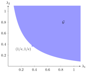
Figure 2: Required signal-to-noise ratios by Algorithm 3 for biclustering.

Remark 7 (Exact biclustering via message passing).

If the assumptions of Theorem 5 hold and the voting condition (62) (respectively, (63)) holds, then $C^{*}_{1}$ (respectively, $C^{*}_{2}$) can be exactly recovered by a voting procedure similar to the one in Algorithm 2. Similar to the analysis in the symmetric case (cf. Fig. 1), whenever (62) – (63) imply the sufficient condition for message passing, i.e., $(\lambda_{1},\lambda_{2})\in{\mathcal{G}}$ defined in (74), there is no computational gap for exact recovery.

To be more precise, consider $K_{i}=\frac{\rho_{i}n}{\log n}$ for $i=1,2$. Then (62) and (63) are equivalent to $\lambda_{i}>8\rho_{i}$. Thus, whenever $K_{1}$ and $K_{2}$ are large enough so that $(8\rho_{1},8\rho_{2})$ lies in the closure $\textbf{cl}({\mathcal{G}})$, or more generally,

$$\left(\liminf_{n\to\infty}\frac{K_{1}\log n_{1}}{n_{1}},\;\liminf_{n\to\infty}\frac{K_{2}\log n_{2}}{n_{2}}\right)\in\frac{1}{8}\textbf{cl}({\mathcal{G}})$$ (75)

then Algorithm 3 plus voting achieves information-theoretically exact recovery threshold with optimal constants (i.e. it is successful if (62) and (63) hold). This result can be viewed as a two-dimensional counterpart of (18) obtained for the symmetric case.

Remark 8.

Clearly $\cal G$ is an open subset of ${\mathbb{R}}_{+}^{2}$ and ${\cal G}$ is an upper closed set. Let $\partial\cal G$ denote its boundary and let $\phi(x)\triangleq\lambda_{2}e^{\lambda_{1}e^{x}}$, so that $\mu_{t+2}^{2}=\phi(\mu_{t}^{2})$ for $t$ even. Note that $(\lambda_{1},\lambda_{2})\in\partial\cal G$ if and only if the function is such that for some $x>0$, $\phi(x)=x$ and $\phi^{\prime}(x)=1.$ Since $\phi^{\prime}(x)=\phi(x)y$, where $y=\lambda_{1}e^{x},$ it follows that $xy=1$ where $y=\lambda_{1}e^{x}$ and $x=\lambda_{2}e^{y}.$ Therefore, it is convenient to express the boundary of ${\mathcal{G}}$ in the parametric form

$$\partial{\cal G}=\{(ye^{-1/y},y^{-1}e^{-y}):y>0\}.$$

It follows that $(1/e,1/e)\in\partial G$ and $\{(\lambda_{1},\lambda_{2})\in{\mathbb{R}}_{+}^{2}:\lambda_{1}\lambda_{2}\geq e^{-2}\}\backslash\{(1/e,1/e)\}\subset{\cal G}.$ Boundaries of ${\mathcal{G}}_{d}$ can be determined similar to (38) (see Fig. 3 for plots).

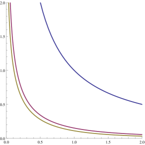
Figure 3: Boundaries of the regions ${\mathcal{G}}_{d}$ for $d=1,2,3$; as $d$ increases, ${\mathcal{G}}_{d}$ converges to ${\mathcal{G}}$ in Fig. 2.

Proof of Theorem 5.

The proof follows step-by-step that of Theorem 1; we shall point out the minor differences. Given $\lambda_{1}$ and $\lambda_{2}$, define

$$d^{\ast}(\lambda_{1},\lambda_{2})=\inf\{d\in{\mathbb{N}}:(\lambda_{1},\lambda_{2})\in{\mathcal{G}}_{d}\},$$ (76)

and choose $c_{0}>0$ so that (79) holds. Given any $\eta\in(0,1)$, choose an arbitrary $\epsilon\in(0,\epsilon_{0})$ such that $\eta(\epsilon)$ defined in (83) is at most $\eta$. Notice that $\epsilon_{0}$ is determined by $c_{0}$. Let $M=8\log(1/\epsilon)$ and choose

$$t^{*}(\lambda_{1},\lambda_{2},M)=\inf\left\{t:\min\{\widehat{\mu}_{t},\widehat{\mu}_{t+1}\}>M\right\}.$$ (77)

In view of Lemma 10 and the assumption that $(\lambda_{1},\lambda_{2})\in{\mathcal{G}}$, $d^{\ast}$ is finite. Since $(\lambda_{1},\lambda_{2})\in{\mathcal{G}}_{d^{*}}$, it follows that $\widehat{\mu}_{t}\to\infty$ and thus $t^{*}(\lambda_{1},\lambda_{2},M)$ is finite.

The assumptions of Theorem 5 imply that $n_{1}\asymp n_{2}.$ Lemmas 3 - 5 therefore go through as before, with $n$ in the upper bounds taken to be $\min\{n_{1},n_{2}\}$, so that $\frac{1}{\sqrt{n_{i}}}\leq\frac{1}{\sqrt{n}}.$ This modification then implies that Lemma 1, justifying the state evolution equations, goes through as before.

The correctness proof for the spectral clean-up procedure in Algorithm 3 is given by Lemma 11 below with $s^{\ast}$ defined by (82); it is similar to Lemma 9 used in Theorem 1 but applies to rectangular matrices and uses singular value decomposition. To ensure that $c_{0}$ is well-defined, the following condition is used for Lemma 11:

$$\frac{\mu\sqrt{K_{1}K_{2}}}{\sqrt{n_{1}}+\sqrt{n_{2}}}=\Omega(1),$$ (78)

which is equivalent to $\min\{\frac{\lambda_{1}K_{2}}{K_{1}},\frac{\lambda_{2}K_{1}}{K_{2}}\}=\Omega(1)$ and implied by the assumptions of Theorem 5, completing the proof of the theorem. (In fact, given the first condition of Theorem 5, i.e., $\lambda_{1},\lambda_{2}$ are fixed, (78) is equivalent to $K_{1}\asymp K_{2}.$) ∎

Lemma 10.

For $d\geq 1$, ${\mathcal{G}}_{d}\subset{\mathcal{G}}_{d+1}$ with ${\mathcal{G}}_{1}=\{(\lambda_{1},\lambda_{2}):\lambda_{1}\lambda_{2}\geq 1\}$, and $\cup_{d=1}^{\infty}{\mathcal{G}}_{d}={\mathcal{G}}$.

Proof.

By definition, $G_{1}(x)=1+x$ and thus for $t$ even, $\widehat{\mu}_{t+2}^{2}=\lambda_{2}(1+\lambda_{1}(1+\widehat{\mu}_{t}^{2}))$. As a consequence, $\widehat{\mu_{t}}\to\infty$ if and only if $\lambda_{1}\lambda_{2}\geq 1$, proving the claim for ${\mathcal{G}}_{1}$. Let $\phi_{d}(x)\triangleq\lambda_{2}G_{d}(\lambda_{1}G_{d}(x))$ so that $\widehat{\mu}^{2}_{t+2}=\phi_{d}(\widehat{\mu}^{2}_{t})$ for $t$ even . The fact ${\mathcal{G}}_{d}\subset{\mathcal{G}}_{d+1}\subset{\mathcal{G}}$ follows from the fact $\phi_{d}(x)$ is increasing in $d$ and $\phi_{d}(x)<\phi(x),$ where $\phi$ is defined in Remark 8. To prove $\cup_{d=1}^{\infty}{\mathcal{G}}_{d}={\mathcal{G}},$ fix $(\lambda_{1},\lambda_{2})\in{\mathcal{G}}.$ It suffices to show that $(\lambda_{1},\lambda_{2})\in{\mathcal{G}}_{d}$ for $d$ sufficiently large. Since $\phi_{2}(x)/x^{4}\to\infty$ as $x\to\infty$, there exists an absolute constant $x_{0}>1$ such that $\phi_{d}(x)\geq x^{2}$ whenever $x\geq x_{0}$ and $d\geq 2.$ Let $t_{0}$ be an even number such that $\mu_{t_{0}}^{2}>x_{0}.$ Since $\phi_{d}(x)$ converges to $\phi(x)$ uniformly on bounded intervals, it follows that the first $t_{0}/2$ iterates using $\phi_{d}$ converge to the corresponding iterates using $\phi.$ So, for $d$ large enough, $\widehat{\mu}_{t_{0}}^{2}>x_{0},$ and hence, for such $d$, $\widehat{\mu}_{t}^{2}\to\infty$ as $t\to\infty,$ so $(\lambda_{1},\lambda_{2})\in{\mathcal{G}}_{d}.$ ∎

Lemma 11.

Suppose (78) holds, i.e.,

$$\frac{\mu\sqrt{K_{1}K_{2}}}{\sqrt{n_{1}}+\sqrt{n_{2}}}\geq\frac{1}{c_{0}}$$ (79)

for some $c_{0}>0$. For $i=1,2$, suppose that $\frac{|C_{i}^{*}|}{K_{i}}\rightarrow 1$ in probability and $\widetilde{C}_{i}$ is a set (possibly depending on $W$) such that

$$\frac{1}{K_{i}}|\widetilde{C}_{i}\cap C_{i}^{\ast}| \geq 1-\epsilon$$ (80)

$$K_{i}(1-\epsilon)\leq|\widetilde{C}_{i}| \leq n_{i}\epsilon$$ (81)

hold for some $0<\epsilon<\epsilon_{0}$, where $\epsilon_{0}$ depends only on $c_{0}$. Let

$$s^{*}=\left(\log\frac{1-\epsilon-3c_{0}\sqrt{h(\epsilon)+\epsilon}}{3c_{0}\sqrt{h(\epsilon)+\epsilon}}\right)^{-1}$$ (82)

where $h(\epsilon)\triangleq\epsilon\log\frac{1}{\epsilon}+(1-\epsilon)\log\frac{1}{1-\epsilon}$ is the binary entropy function. Then $\widehat{C}_{i}$ returned by Algorithm 3 satisfies $|\widehat{C}_{i}\cap C^{\ast}_{i}|\geq(1-\eta(\epsilon))K_{i}$ for $i=1,2$, with probability converging to one as $n\to\infty,$ where

$$\eta(\epsilon)=2\epsilon+650c_{0}^{2}\;\frac{h(\epsilon)+\epsilon}{(1-\epsilon)^{2}}.$$ (83)

Proof.

(Similar to proof of Lemma 9.) We prove the lemma for $\widehat{C}_{1}$; the proof for $\widehat{C}_{2}$ is identical. For the first part of the proof we assume that for $i=1,2$, $\widetilde{C}_{i}$ is fixed, and later use a union bound over all possible choices of $\widetilde{C}_{i}.$ Recall that $W_{\widetilde{C}_{1}\widetilde{C}_{2}}$, which we abbreviate henceforth as $\widetilde{W}$, is the matrix $W$ restricted to entries in $\widetilde{C}_{1}\times\widetilde{C}_{2}$. Let $Z=\widetilde{W}-\mathbb{E}[\widetilde{W}]$ and note that

$$\mathbb{E}[\widetilde{W}]=\mu\sqrt{|\widetilde{C}_{1}\cap C_{1}^{*}||\widetilde{C}_{2}\cap C_{2}^{*}|}v_{1}v_{2}^{\top}$$ (84)

is a rank-one matrix, where $v_{i}$ is the unit vector in ${\mathbb{R}}^{|\widetilde{C}_{i}|}$ obtained by normalizing the indicator vector of $\widetilde{C}_{i}\cap C^{*}_{i}.$ Thus, thanks to (80), the leading singular value of $\mathbb{E}[\widetilde{W}]$ is at least $\mu\sqrt{K_{1}K_{2}}(1-\epsilon)$ with left singular vector $v_{1}$ and right singular vector $v_{2}$.

It is well-known (see, e.g., [26, Corollary 5.35]) that if $M$ is an $m_{1}\times m_{2}$ matrix with i.i.d. standard normal entries, then $\mathbb{P}\left\{\|M\|\geq\sqrt{m_{1}}+\sqrt{m_{2}}+t\right\}\leq 2e^{-t^{2}/2}.$ Applying this result for $m_{i}=|\widetilde{C}_{i}|$, which satisfies $m_{i}\leq\epsilon n_{i}$ by (81), and $t=2\sqrt{h(\epsilon)(n_{1}+n_{2})}$, we have for fixed $(\widetilde{C}_{1},\widetilde{C}_{2})$,

$$\mathbb{P}\left\{\|Z\|\geq(\sqrt{n_{1}}+\sqrt{n_{2}})\beta\right\}\leq 2e^{-2(n_{1}+n_{2})h(\epsilon)},$$

where $\beta\triangleq 3\sqrt{\epsilon+h(\epsilon)})$. Similar to the proof of Lemma 9, the number of $(\widetilde{C}_{1},\widetilde{C}_{2})$ that satisfies (81) is at most $e^{(n_{1}+n_{2})h(\epsilon)}$. By union bound, if we drop the assumption that $\widetilde{C}_{i}$ is fixed for $i=1,2$, we still have that with high probability, $\|Z\|\leq(\sqrt{n_{1}}+\sqrt{n_{2}})\beta$.

Denote by $u$ the leading left singular vector of $W_{\widetilde{C}_{1}\widetilde{C}_{2}}$. Then

$$\|uu^{\top}-v_{1}v_{1}^{\top}\|_{\rm F}= ~{}\sqrt{2}\|(\mathbf{I}-uu^{\top})v_{1}v_{1}^{\top}\|_{\rm F}\overset{(a)}{=}\sqrt{2}\|(\mathbf{I}-uu^{\top})v_{1}v_{1}^{\top}\|$$

$$\overset{(b)}{\leq} ~{}\sqrt{2}\min\left\{\frac{\|Z\|}{|\sigma_{1}(\mathbb{E}[\widetilde{W}])-\sigma_{2}(\widetilde{W})|},1\right\}\overset{(c)}{\leq}\frac{2\sqrt{2}\|Z\|}{\sigma_{1}(\mathbb{E}[\widetilde{W}])},$$

where (a) is because $\text{rank}((\mathbf{I}-uu^{\top})v_{1}v^{\top}_{1})\leq 1$, (b) follows from Wedin’s sin-$\theta$ theorem for SVD [27], (c) follows from Weyl’s inequality $\sigma_{2}(\widetilde{W})\leq\sigma_{2}(\mathbb{E}[\widetilde{W}])+\|Z\|=\|Z\|$. In view of (84), conditioning on the high-probability event that $\|Z\|\leq(\sqrt{n_{1}}+\sqrt{n_{2}})\beta$, we have

$$\|uu^{\top}-v_{1}v_{1}^{\top}\|_{\rm F}\leq\frac{2\sqrt{2}\beta(\sqrt{n_{1}}+\sqrt{n_{2}})}{\mu(1-\epsilon)\sqrt{K_{1}K_{2}}}\leq\frac{2\sqrt{2}c_{0}\beta}{1-\epsilon},$$ (85)

where the last inequality follows from the standing assumption (79).

Next, we argue that $\widehat{u}$ is close to $u$, and hence, close to $v_{1}$ by the triangle inequality. By (50), the initial value $u^{0}\in{\mathbb{R}}^{\widetilde{C}_{1}}$ satisfies $|\langle u,u^{0}\rangle|\geq(2\sqrt{n_{1}\log n_{1}})^{-1}$ with high probability. By Weyl’s inequality, the largest singular value of $\widetilde{W}$ is at least $\mu\sqrt{K_{1}K_{2}}(1-\epsilon)-(\sqrt{n_{1}}+\sqrt{n}_{2})\beta$, and the other singular values are at most $(\sqrt{n_{1}}+\sqrt{n}_{2})\beta$. In view of (79), $\frac{1-\epsilon}{c_{0}\beta}-1>1$ for all $\epsilon<\epsilon_{0}$, where $\epsilon_{0}>0$ depends only on $c_{0}$. Let $\lambda_{1}$ and $\lambda_{2}$ denote the first and second eigenvalue of $\widetilde{W}\widetilde{W}^{\top}$ in absolute value, respectively. Let $r=\lambda_{2}/\lambda_{1}$. Then $r\leq(\frac{c_{0}\beta}{1-\epsilon-c_{0}\beta})^{2}$. Since for even $t$, $u^{t}=(\widetilde{W}\widetilde{W}^{\top})^{t/2}u^{0}/\|(\widetilde{W}\widetilde{W}^{\top})^{t/2}u^{0}\|$, the same analysis of power iteration that leads to (52) yields

$$\langle u^{t},u\rangle^{2}\geq 1-\frac{r^{t}}{\langle u,u^{0}\rangle^{2}-2|\langle u,u^{0}\rangle|r^{t/2}}.$$

Since $\widehat{u}=u^{2\lceil s^{*}\log n\rceil}$ and $s^{*}=(\log\frac{1-\epsilon-c_{0}\beta}{c_{0}\beta})^{-1}$, we have $r^{\lceil s^{*}\log n_{1}\rceil}\leq n_{1}^{-2}$ and thus $|\langle\widehat{u},u\rangle^{2}|\geq 1-n_{1}^{-1}$ and consequently, $\|uu^{\top}-\widehat{u}(\widehat{u})^{\top}\|_{\rm F}^{2}=2-2\left\langle u,\widehat{u}\right\rangle^{2}\leq n_{1}^{-1}$. Similar to (53), applying (85) and the triangle inequality, we obtain

$$\min\{\|\widehat{u}-v_{1}\|,\|\widehat{u}+v_{1}\|\}\leq\|\widehat{u}(\widehat{u})^{\top}-v_{1}v_{1}^{\top}\|_{\rm F}\leq\frac{2\sqrt{2}c_{0}\beta}{1-\epsilon}+n_{1}^{-1/2}\leq\frac{3c_{0}\beta}{1-\epsilon}\triangleq\beta_{0}.$$ (86)

By the same argument that proves (54), we have $\limsup_{n\rightarrow\infty}|C_{1}^{*}\triangle\widehat{C}_{1}|/{K_{1}}\leq 2\epsilon+8\beta_{0}^{2}\leq\eta(\epsilon)$ with $\eta$ defined in (83), completing the proof. ∎

Remark 9.

Condition (78) implies that $\mu^{2}K_{1}K_{2}/n_{1}=\Omega(1)$, which in turn implies that (61) holds in the regime $K_{1}=o(n_{1})$. Hence, under (78), either both $C^{*}_{1}$ and $C^{*}_{2}$ can be weakly recovered or neither of them can be weakly recovered.

Appendix A Row-wise thresholding

We describe a simple thresholding procedure for recovering $C^{*}$. Let $R_{i}=\sum_{j}W_{i,j}$ for $i\in[n].$ Then $R_{i}\sim{\cal N}(K\mu,n)$ if $i\in C^{*}$ and $R_{i}\sim{\cal N}(0,n)$ if $i\notin C^{\ast}$. Let $\widehat{C}=\left\{i\in[n]:R_{i}\geq\frac{K\mu}{2}\right\}.$ Then $\mathbb{E}\left[|\widehat{C}\triangle C^{*}|\right]=nQ\left(\frac{K\mu}{2\sqrt{n}}\right).$ Recall that $\lambda=\frac{K^{2}\mu^{2}}{n}$. Hence, if

$$\lambda=\omega\left(\log\frac{n}{K}\right),$$ (87)

then we have $\mathbb{E}[|\widehat{C}\triangle C^{*}|]=o(K)$ and hence achieved weak recovery. In the regime $K\asymp n\asymp(n-K),$ $\lambda=\omega(\log\frac{n}{K})$ is equivalent to $\lambda\to\infty$, which is also equivalent to $K\mu^{2}\to\infty$ and coincides with the necessary and sufficient condition for the information-theoretic possibility of weak recovery in this regime [13, Theorem 2]. (If instead $n-K=o(n)$, weak recovery is trivially provided by $\widehat{C}=[n]$.) Thus, row-wise thresholding provides weak recovery in the regime $K\asymp n\asymp(n-K)$ whenever information theoretically possible. Under the information-theoretic condition (14), an algorithm attaining exact recovery can be built using row-wise thresholding for weak recovery followed by voting, as in Algorithm 2 (see [13, Theorem 4] and its proof). In the regime $\frac{n}{K}\log\frac{n}{K}=o(\log n)$, or equivalently $K=\omega(n\log\log n/\log n)$, condition (14) implies that $\lambda=\omega(\log\frac{n}{K})$, and hence in this regime exact recovery can be attained in linear time $O(n^{2})$ whenever information theoretically possible.

Appendix B Proofs of Theorems 3 and 4

In the proofs below we use the following notation. We write $\textsf{p}_{e}(\pi_{1},s^{2})$ to denote the minimal average error probability for testing ${\cal N}(\mu_{1},\sigma^{2})$ versus ${\cal N}(\mu_{0},\sigma^{2})$ with priors $\pi_{1}$ and $1-\pi_{1}$, where $\mu_{1}\geq\mu_{0}$ and $s^{2}=\frac{(\mu_{0}-\mu_{1})^{2}}{\sigma^{2}}.$ That is,

$$\textsf{p}_{e}(\pi_{1},s^{2})\triangleq\min_{\gamma}\{\pi_{1}Q(s-\gamma)+(1-\pi_{1})Q(\gamma)\}.$$

Proof of Theorem 3.

We defer the proof of (i) to the end and begin with the proof of (ii). Column sum thresholding for recovery of $C_{2}^{*}$ consists of comparing $\sum_{i}W_{i,j}$ to a threshold for each $j\in[n_{2}]$ to estimate whether $j\in C_{2}^{*}.$ This sum has the ${\cal N}(K_{1}\mu,n_{1})$ distribution if $j\in C_{2}^{*}$, which has prior probability $K_{2}/n_{2}$, and the sum has the ${\cal N}(0,n_{1})$ distribution otherwise. The mean number of classification errors divided by $K_{2}$ is given by $(n_{2}/K_{2})\textsf{p}_{e}(K_{2}/n_{2},K_{1}^{2}\mu^{2}/n_{1}),$ which converges to zero under (59). This proves (ii).

The proof of (iii) is similar, although it involves the method of successive withholding in a way similar to that in Algorithm 2. The set $[n_{1}]$ is partitioned into sets, $S_{1},\ldots,S_{1/\delta}$ of size $n_{1}\delta.$ There are $1/\delta$ rounds of the algorithm, and indices in $S_{\ell}$ are classified in the $\ell^{th}$ round. For the $\ell^{th}$ round, by assumption, given $\epsilon>0,$ there exists an estimator $\widehat{C}_{2}$ based on observation of $W$ with the rows indexed by $S_{\ell}$ hidden such that $|\widehat{C}_{2}\Delta C^{*}_{2}|\leq\epsilon K_{2}$ with high probability. Then the voting procedure estimates whether $i\in C_{1}^{*}$ for each $i\in S_{\ell}$ by comparing $\sum_{j\in\widehat{C}_{2}}W_{i,j}$ to a threshold for each $i\in[n_{1}]$. This sum has approximately the ${\mathcal{N}}(K_{2}\mu,K_{2})$ distribution if $i\in C_{1}^{*}$ and ${\mathcal{N}}(0,K_{2})$ distribution otherwise ; the discrepancy can be made sufficiently small by choosing $\epsilon_{2}$ to be small (See [13, Lemma 9] for a proof). Thus, the mean number of classification errors divided by $K_{1}$ is well approximated by $(n_{1}/K_{1})\textsf{p}_{e}(K_{1}/n_{1},K_{2}\mu^{2})$, which converges to zero under (61), completing the proof of (iii).

Now to the proof of (i). The proof of sufficiency for weak recovery is closely based on the proof of sufficiency for exact recovery by the MLE given in [2]; the reader is referred to [2] for the notation used in this paragraph. The proof in [2] is divided into two sections. In our terminology, [2, Section 3.1] establishes the weak recovery of $C_{1}^{*}$ and $C_{2}^{*}$ by the MLE under the assumptions (57), (62), and (63). However, the assumption (62) (and similarly, (63)) is used in only one place in the proof, namely for bounding the terms $T_{1,km}$ defined therein. We explain here why (57) alone is sufficient for the proof of weak recovery. Condition (57) implies condition (61), which, in the notation of [2], implies that there exists some sufficiently small $\alpha>0$ such that

$$\frac{a^{2}m}{2\log(N/n)}\geq 1+\alpha.$$

So [2, (3.4)] can be replaced as: there exist some sufficiently small $\delta_{1}>0$ and $\alpha_{1}>0$ such that

$$\frac{(1-\delta_{1})^{2}}{2}a^{2}m\geq(1+\alpha_{1})\log(N/n)\geq(1+\alpha_{1})\log\left(\frac{\delta(N-n)}{n-k}\right),$$

where we use the assumption $0\leq k<(1-\delta)n$, or $n-k>\delta n.$ Thus, for large enough $n,$

$$T_{1,km} \leq\exp\left(-\frac{\delta n\alpha_{1}}{2}\left(\log\left(\frac{N-n}{n-k}\right)\right)\right)\leq\exp\left(-\frac{\delta n\alpha_{1}}{2}\log\left(\frac{N-n}{n}\right)\right)=o(1/n),$$

from which the desired conclusion, $\sum_{k:(n-k)>\delta n}T_{1,km}=o(1),$ follows. This completes the proof of sufficiency of (57) for weak recovery of both $C_{1}^{*}$ and $C_{2}^{*}$, and marks the end of our use of notation from [2].

The rate distortion argument used in the proof of [13, Theorem 5] shows that (58) must hold if $C_{1}^{*}$ and $C_{2}^{*}$ are both weakly recoverable. ∎

Proof of Theorem 4.

The proof follows along the lines of the proofs of Theorem 3 parts (ii) and (iii). The key calculation for part (i) is that (62) implies that $n_{1}\textsf{p}_{e}(K_{1}/n_{1},K_{2}\mu^{2})\to 0;$ and the key calculation for part (ii) is that (64) implies that $n_{2}\textsf{p}_{e}(K_{2}/n_{2},K_{1}^{2}\mu^{2}/n_{1})\to 0.$ ∎

References

- [1] R. B. Ash. Information Theory. Dover Publications Inc., New York, NY, 1965.
- [2] C. Butucea, Y. Ingster, and I. Suslina. Sharp variable selection of a sparse submatrix in a high-dimensional noisy matrix. ESAIM: Probability and Statistics, 19:115–134, June 2015.
- [3] C. Butucea and Y. I. Ingster. Detection of a sparse submatrix of a high-dimensional noisy matrix. Bernoulli, 19(5B):2652–2688, 11 2013.
- [4] T. T. Cai, T. Liang, and A. Rakhlin. Computational and statistical boundaries for submatrix localization in a large noisy matrix. arXiv:1502.01988, Feb. 2015.
- [5] T. T. Cai, Z. Ma, and Y. Wu. Optimal estimation and rank detection for sparse spiked covariance matrices. Probability Theory and Related Fields, 161(3-4):781–815, Apr. 2015.
- [6] Y. Chen and J. Xu. Statistical-computational tradeoffs in planted problems and submatrix localization with a growing number of clusters and submatrices. In Proceedings of ICML 2014 (Also arXiv:1402.1267), Feb 2014.
- [7] K. Chung. A course in probability theory. Academic press, 2nd edition, 2001.
- [8] A. Condon and R. M. Karp. Algorithms for graph partitioning on the planted partition model. Random Struct. Algorithms, 18(2):116–140, Mar. 2001.
- [9] H. David and H. Nagaraja. Order Statistics. Wiley-Interscience, Hoboken, New Jersey, USA, 3 edition, 2003.
- [10] K. Davidson and S. Szarek. Local operator theory, random matrices and Banach spaces. In W. Johnson and J. Lindenstrauss, editors, Handbook on the Geometry of Banach Spaces, volume 1, pages 317–366. Elsevier Science, 2001.
- [11] Y. Deshpande and A. Montanari. Finding hidden cliques of size in nearly linear time. Foundations of Computational Mathematics, 15(4):1069–1128, August 2015.
- [12] D. Féral and S. Péché. The largest eigenvalue of rank one deformation of large Wigner matrices. Communications in mathematical physics, 272(1):185–228, 2007.
- [13] B. Hajek, Y. Wu, and J. Xu. Information limits for recovering a hidden community. arXiv:1509.07859, September 2015.
- [14] B. Hajek, Y. Wu, and J. Xu. Semidefinite programs for exact recovery of a hidden community. draft, September 2015.
- [15] J. A. Hartigan. Direct clustering of a data matrix. Journal of the American Statistical Association, 67(337):123–129, 1972.
- [16] W. Hoeffding. Probability inequalities for sums of bounded random variables. Journal of the American Statistical Association, 58(301):13–30, 1963.
- [17] A. Knowles and J. Yin. The isotropic semicircle law and deformation of Wigner matrices. Communications on Pure and Applied Mathematics, 66(11):1663–1749, 2013.
- [18] M. Kolar, S. Balakrishnan, A. Rinaldo, and A. Singh. Minimax localization of structural information in large noisy matrices. In Advances in Neural Information Processing Systems, 2011.
- [19] Z. Ma and Y. Wu. Computational barriers in minimax submatrix detection. The Annals of Statistics, 43(3):1089–1116, 2015.
- [20] A. Montanari, D. Reichman, and O. Zeitouni. On the limitation of spectral methods: From the Gaussian hidden clique problem to rank one perturbations of Gaussian tensors. ArXiv 1411.6149, Nov. 2014.
- [21] E. Mossel, J. Neeman, and A. Sly. Consistency thresholds for the planted bisection model. In Proceedings of the Forty-Seventh Annual ACM on Symposium on Theory of Computing, STOC ’15, pages 69–75, New York, NY, USA, 2015. ACM.
- [22] E. Mossel, J. Neeman, and S. Sly. Belief propagation, robust reconstruction, and optimal recovery of block models (extended abstract). In JMLR Workshop and Conference Proceedings (COLT proceedings), volume 35, pages 1–35, 2014.
- [23] V. V. Petrov. Limit theorems of probability theory: Sequences of independent random variables. Oxford Science Publications, Clarendon Press, Oxford, United Kingdom, 1995.
- [24] A. A. Shabalin, V. J. Weigman, C. M. Perou, and A. B. Nobel. Finding large average submatrices in high dimensional data. The Annals of Applied Statistics, 3(3):985–1012, 2009.
- [25] G. Szegö. Orthogonal polynomials. American Mathematical Society, Providence, RI, 4th edition, 1975.
- [26] R. Vershynin. Introduction to the non-asymptotic analysis of random matrices. Arxiv preprint arxiv:1011.3027, 2010.
- [27] P. Wedin. Perturbation bounds in connection with singular value decomposition. BIT Numerical Mathematics, 12(1):99–111, 1972.