Published in PRL 20 January 2016]
BICEP2 / Keck Array VI: Improved Constraints On Cosmology and Foregrounds When Adding 95 GHz Data From Keck Array
Abstract
We present results from an analysis of all data taken by the BICEP2 & Keck Array CMB polarization experiments up to and including the 2014 observing season. This includes the first Keck Array observations at 95 GHz. The maps reach a depth of 50 nK deg in Stokes and in the 150 GHz band and 127 nK deg in the 95 GHz band. We take auto- and cross-spectra between these maps and publicly available maps from WMAP and Planck at frequencies from 23 GHz to 353 GHz. An excess over lensed-CDM is detected at modest significance in the 95150 spectrum, and is consistent with the dust contribution expected from our previous work. No significant evidence for synchrotron emission is found in spectra such as 2395, or for correlation between the dust and synchrotron sky patterns in spectra such as 23353. We take the likelihood of all the spectra for a multi-component model including lensed-CDM, dust, synchrotron and a possible contribution from inflationary gravitational waves (as parametrized by the tensor-to-scalar ratio ), using priors on the frequency spectral behaviors of dust and synchrotron emission from previous analyses of WMAP and Planck data in other regions of the sky. This analysis yields an upper limit at 95% confidence, which is robust to variations explored in analysis and priors. Combining these -mode results with the (more model-dependent) constraints from Planck analysis of CMB temperature plus BAO and other data, yields a combined limit at 95% confidence. These are the strongest constraints to date on inflationary gravitational waves.
pacs:
98.70.Vc, 04.80.Nn, 95.85.Bh, 98.80.Esxyz
Introduction.—Measurements of the cosmic microwave background (CMB) Penzias and Wilson (1965) are one of the observational pillars of the standard cosmological model (CDM) and constrain its parameters to high precision (see most recently Ref. Planck Collaboration 2015 XIII (2015)). This model extrapolates the Universe back to very high temperatures ( K) and early times ( s). Observations indicate that conditions at these early times are described by an almost uniform plasma with a nearly scale invariant spectrum of adiabatic density perturbations. However, CDM itself offers no explanation for how these conditions occurred. The theory of inflation is an extension to the standard model, which postulates a phase of exponential expansion at a still earlier epoch ( s) that precedes CDM and produces the required initial conditions (See Ref. Kamionkowski and Kovetz (2015) for a recent review and citations to the original literature.)
There is widespread support for the claim that existing observations already indicate that some version of inflation probably did occur, but there are also skeptics Guth et al. (2014); Ijjas et al. (2014). As well as the specific form of the initial density perturbations there is an additional relic which inflation predicts, and which one can attempt to detect. Inflation launches tensor mode perturbations into the fabric of space-time which will propagate unimpeded as inflationary gravitational waves (IGWs) to the present day. Their amplitude is diminished with the expansion of the Universe, and detection at the present epoch is not feasible with current technology. The most promising potential method of detection is to look for their signature written into the pattern of the CMB at last scattering, 380,000 years after the Universe entered the realm of fully known physics. Inflationary theories generically predict that IGWs exist, but many specific models have been proposed producing a wide range of amplitudes—with some being unobservably small Kamionkowski and Kovetz (2015). The size of the IGW signal is conventionally expressed as the initial ratio of the tensor and scalar perturbation amplitudes .
In the CDM standard model the CMB is polarized by Thomson scattering of Doppler induced quadrupoles in the local radiation field at last scattering. This naturally produces a polarization pattern with direction parallel/perpendicular to the gradient of its intensity—this is curl-free, or -mode polarization, and was first detected in Ref. Kovac et al. (2002). Due to small gravitational deflections of the CMB photons in flight by intervening large scale structure, the initial purity of the -mode pattern is disturbed and a small lensing -mode is produced at sub-degree angular scales Polarbear Collaboration (2014); Keisler et al. (2015).
IGWs are intrinsically quadrupolar distortions of the metric and produce both and -mode polarization depending on their orientation with respect to our last scattering surface. However, due to the large CDM -mode signal, the most promising place to search for an IGW signal is in -modes. Furthermore, since the IGW -modes have a much redder spectrum than the lensing -modes, the best place to look is at angular scales larger than a few degrees (multipoles ). Limits on IGW from non-polarized CMB observations are now fully saturated at cosmic variance limits Planck Collaboration 2015 XIII (2015) and it is generally agreed that the best (only) way to make further progress is through improved measurements of CMB -modes.
The BICEP and Keck Array telescopes are small aperture polarimeters specifically designed to search for an IGW signal at the recombination bump (). BICEP1 operated from 2006 to 2008 and set a limit at 95% confidence (BICEP1 Collaboration, 2014). BICEP2 operated from 2010 to 2012 at 150 GHz and in Ref. BICEP2 Collaboration I (2014) reported a detection of a substantial excess over the lensed-CDM expectation in the multipole range . Additional measurements at 150 GHz taken by the Keck Array during 2012 and 2013 confirmed this excess (Keck Array and BICEP2 Collaborations V, 2015). However, new data from the Planck space mission provided evidence that emission from galactic dust grains could be more polarized at high galactic latitudes than anticipated (Planck Collaboration Int. XIX, 2015; Planck Collaboration Int. XXX, 2014), a possibility emphasized by (Flauger et al., 2014; Mortonson and Seljak, 2014). Analysis of the combined BICEP2 and Keck Array 150 GHz data in combination with data from Planck (principally at 353 GHz) showed that a substantial part of the 150 GHz excess is due to polarized emission from galactic dust grains, and that once this is accounted for, the result becomes at 95% confidence (BICEP2/Keck and Planck Collaborations, 2015).
BICEP2 was a simple 26 cm aperture all-cold refractor, and Keck Array is basically five copies of this on a single telescope mount (BICEP2 Collaboration II, 2014; Keck Array and BICEP2 Collaborations V, 2015). Both are sited at the South Pole in Antarctica, taking advantage of the dry atmosphere and stable observing conditions. In addition to the all-cold optics these telescopes have two features which aid greatly in the suppression and characterization of instrumental systematics: i) they are equipped with co-moving absorptive forebaffles resulting in extremely low far side-lobe response, and ii) the entire instrument can be rotated about the line of sight allowing modulation of polarized signal.
Keck Array was designed at the outset to observe in multiple frequency bands—the 2012 and 2013 observations were all taken at 150 GHz because detectors for other bands were not yet ready. Before the 2014 season two of the five receivers of Keck Array were refitted for operation in a band centered on 95 GHz (the other three receivers remaining unchanged at 150 GHz). In this paper we fold in this new data and perform a multi-component, multi-spectral likelihood analysis similar to our previous analysis BICEP2/Keck and Planck Collaborations (2015).
This paper builds on the initial BICEP2 results paper (BICEP2 Collaboration I, 2014, hereafter BK-I), the Keck 2012+2013 results paper (Keck Array and BICEP2 Collaborations V, 2015, hereafter BK-V), and the BICEP2/Keck/Planck analysis paper (BICEP2/Keck and Planck Collaborations, 2015, hereafter BKP).
Instrument and observations.—The Keck Array instrument is described in Sec. 2 of BK-V. (See also the BICEP2 Instrument Paper BICEP2 Collaboration II (2014) for further details.) Before the 2014 observing season two of the receivers of Keck Array were removed, the lenses and filters were replaced with versions optimized for a band centered at 95 GHz, and the focal planes were replaced with units loaded with appropriately scaled versions of our antenna-coupled detectors (BICEP2/Keck and Spider Collaborations, 2015). Because the physical size of these antennas is larger each of the four tiles contains only a array (rather than at 150 GHz). With two focal planes at 95 GHz this gives 288 total detector pairs (576 total detectors).
During the 2014 austral winter season the array was operated exactly as for the previous seasons. A % region of sky centered at RA 0h, Dec. was observed from March until November over fifty minute “scansets”. Efficiency and yield was similar to previous seasons. See Sec. 4 of BK-V for further details of the observing strategy and data selection.
BICEP2/Keck Maps.—The processing from time stream to maps is identical to that described in Sec. III & IV of BK-I and summarized in Sec. 5 of BK-V. Relative gain calibration is applied between the two halves of each pair and the difference is taken. Filtering is then applied to remove residual atmospheric noise and any ground-fixed (scan-synchronous) pickup. The data are then binned into simple map pixels and, with knowledge of the polarization sensitivity directions, maps of Stokes parameters and are formed. “Deprojection” is also performed to remove leakage of temperature to polarization due to beam systematics and this results in an additional filtering of signal.
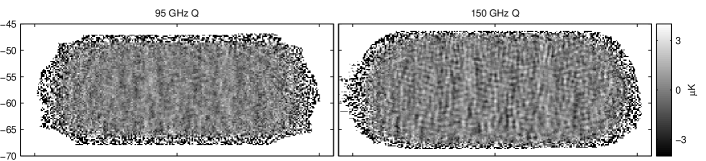
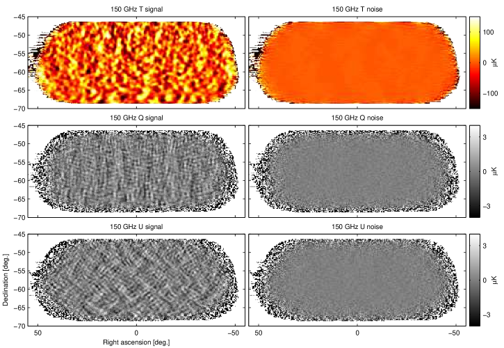
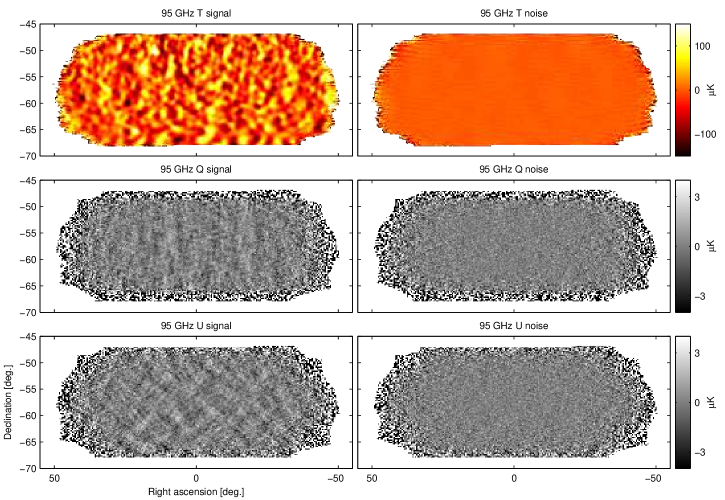
Fig. 1 shows the 95 & 150 GHz maps combining data from BICEP2 (2010–2012) and Keck Array (2012–2014)—we refer to these as the BK14 maps meaning that they contain all data up to and including that taken during the 2014 observing season. The 150 GHz maps add 3 more receiver years to the previous 13 in the BK13 based analysis of BKP, and modestly improves the / sensitivity from 57 nK deg to 50 nK deg (3.0 K arcmin) over an effective area of 395 square degrees. These are the deepest maps of CMB polarization published to date. The 95 GHz maps contain only 2 receiver years of data and the / sensitivity is 127 nK deg (7.6 K arcmin) over an effective area of 375 square degrees. (The survey weight is thus 310,000 (47,000) K-2 at 150 (95) GHz.) The 95 GHz beam is wider (43 arcmin versus 30 arcmin FWHM) and we see the effect of the additional beam smoothing. However, the degree scale structure is clearly nearly identical at both frequencies. While there is a dust component hidden in the 150 GHz maps it is highly subdominant to CDM -mode signal. See Appendix A for the full set of // signal and noise maps.
External Maps.—We use the Public Release 2 “full mission” maps available from the Planck Legacy Archive 111See http://www.cosmos.esa.int/web/planck/pla (Planck Collaboration 2015 I, 2015), noting that these are nearly identical to those used in BKP. For this analysis we also add the WMAP9 23 GHz (K-band) and 33 GHz (Ka-band) maps 222See http://lambda.gsfc.nasa.gov/product/map/dr5/m_products.cfm(Bennett et al., 2013).
For each of these external maps we deconvolve the native instrument beam, reconvolve the Keck 150 GHz beam, and then process the result through an “observing” matrix to produce a map with the same filtering of spatial modes as the 150 GHz map. See Sec. II.A of BKP for further details of this process. For Planck we use the FFP8 simulations (Planck Collaboration 2015 XII, 2015) and for WMAP we use simple inhomogeneous white noise simulations derived from the provided variance maps.
Power Spectra.—We convert the maps to power spectra using the methods described in Sec. VI of BK-I including the matrix based purification operation to prevent to mixing. We generate separate purification matrices to match the filtering of the 95 & 150 GHz maps.
We first subject the new 95 GHz data to our usual suite of “jackknife” internal consistency checks. The results are given in Appendix B and show empirically that the data are free of systematic contamination at a level greater than the noise. In addition, in Appendix C we investigate the stability of the previous 150 GHz spectrum when adding the new 2014 data—there is no indication of problems.
We now proceed to comparing the spectra and cross spectra of our 95 and 150 GHz maps—Fig. 2 shows the results. We use a common apodization mask as the geometric mean of the two (smoothed) inverse variance maps. The spectra agree to within much better than the nominal error bar size because the uncertainty is dominated by sample variance and we are observing the same piece of sky. To make a rough estimate of the significance of deviation from lensed-CDM, we calculate and (sum of normalized deviations) as shown on the plot. We see strong evidence for excess power in BK14BK14150 and moderate evidence in BK14BK14150. Dashed lines for the lensed-CDM+dust model derived in BKP are over-plotted and appear to be consistent with the new data.
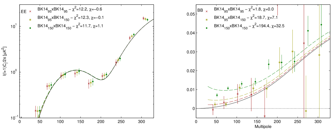
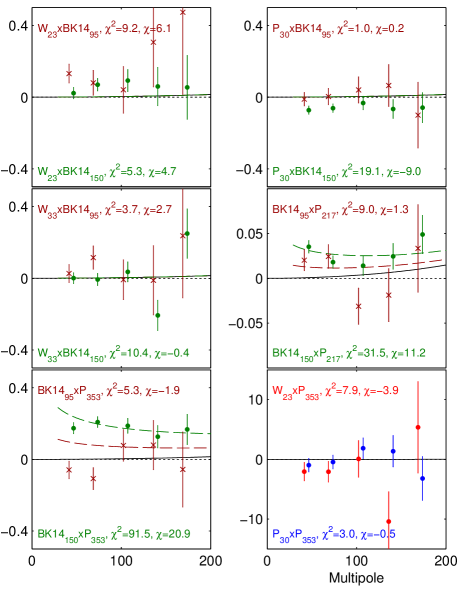
Fig. 3 shows selected cross spectra between the BK14 95 & 150 GHz maps and the Planck (P) and WMAP (W) bands. There is no strong evidence for detection of synchrotron emission—WBK1495 and WBK14150 are both mildly elevated but PBK14150 has stronger nominal anticorrelation (as noted in the BKP paper). WBK1495 and WBK14150 are both consistent with null. The only strong detections of excess signal are in BK14P353 and, at lower significance BK14P217. See Appendix D for the full set of auto- and cross-spectra.
Likelihood Analysis.—We next proceed to a multicomponent, multi-spectral likelihood analysis which is an expanded version of that described in Sec. III of the BKP paper. We compute the likelihood of the data for any given proposed model using an extended version of the HL approximation (Hamimeche and Lewis, 2008) and the full covariance matrix of the auto- and cross-spectral bandpowers as derived from simulations (setting to zero terms whose expectation value is zero).
In this analysis we primarily use a lensed-CDM+dust+synchrotron+ model and explore the parameter space using COSMOMC (Lewis and Bridle, 2002). The COSMOMC module containing the data and model is available for download at http://bicepkeck.org. In this paper the “baseline” analysis is defined to:
-
•
Use the BK14 maps as shown in Fig. 1 (all BICEP2/Keck data up to and including that taken during the 2014 observing season).
-
•
Use all the polarized bands of Planck (30–353 GHz) plus the 23 & 33 GHz bands of WMAP.
- •
-
•
Use nine bandpowers spanning the range .
-
•
Include dust with amplitude evaluated at 353 GHz and . As in the BKP analysis the frequency spectral behavior is taken as a simple modified black body spectrum with K and , using a Gaussian prior with the given width. Analyzing polarized emission at intermediate galactic latitudes Fig. 11 of Ref. Planck Collaboration Int. XXII (2015) shows that this model is accurate in the mean to within a few percent over the frequency range 100–353 GHz, while the patch-to-patch fluctuation is noise dominated. The spatial power spectrum is taken as a simple power law marginalizing over the range , where .
-
•
Include synchrotron with amplitude evaluated at 23 GHz (the lowest WMAP band) and , assuming a simple power law for the frequency spectral behavior with a Gaussian prior (Fuskeland et al., 2014). The spatial power spectrum is taken as a simple power law marginalizing over the range .
-
•
Allow sync/dust correlation and marginalize over the correlation parameter .
-
•
Quote the tensor/scalar power ratio at a pivot scale of 0.05 Mpc-1 and fix the tensor spectral index .
See Appendix E1 for a more detailed explanation of these choices.
Results of this baseline analysis are shown in Fig. 4 and yield the following statistics: , at 95% confidence, K2, and K2 at 95% confidence. For the zero-to-peak likelihood ratio is 0.63. Taking , where is the CDF (for one degree of freedom), we estimate that the probability to get a likelihood ratio smaller than this is 18% if, in fact, . Running the analysis on the lensed-CDM+dust+noise simulations produces a similar number. The zero-to-peak likelihood ratio for indicates that the detection of dust is now .
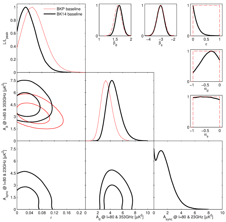
Results for the additional parameters are shown in the upper right part of Fig. 4. The dust frequency spectral parameter pulls weakly against the prior to higher values. The synchrotron frequency spectral parameter just reflects the prior (as expected since synchrotron is not strongly detected). The data have a mild preference for values of close to the found in Ref. Planck Collaboration Int. XXX (2014), while is unconstrained. The data disfavor strong sync/dust correlation (due to the non detection of signal in spectra like P353—see Fig 3). As approaches zero becomes unconstrained leading to an increase in the available parameter volume, and the “flare” in the constraints.
The maximum likelihood model (including priors) has parameters , K2, K2, , , , , and . This model appears to be an acceptable fit to the data—see Appendix D for further details.
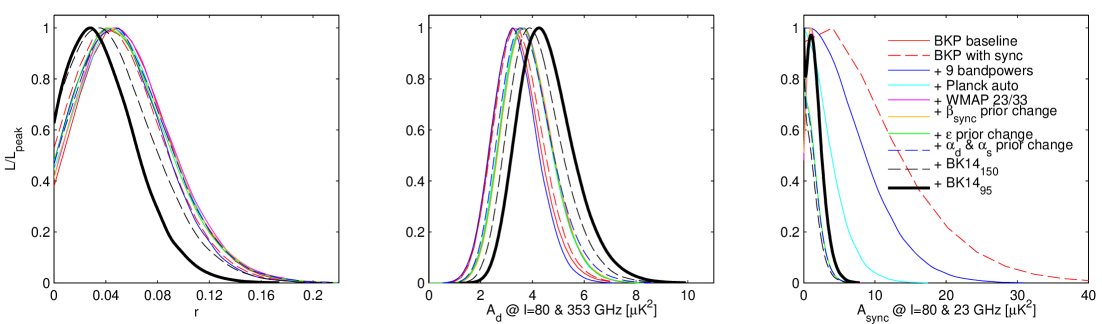
In Fig. 4 we see that as compared to the primary BKP analysis the peak position of the likelihood curve for has shifted down slightly. In Fig. 5 we investigate why. Although we have made extensive changes to the model, these make only a small difference. (See Appendix E1 for details of these changes.) The change from the BK13150 to the BK14150 maps causes some of the downward shift in the peak position. This may seem surprising given that only a relatively small amount of additional data has been added (%). However Appendix C shows that the shifts in the bandpower values are not unlikely and we should therefore accept the shift in the constraint as simply due to noise fluctuation. Adding in the BK1495 data produces an additional downward shift in the peak position, and also significantly narrows the likelihood curve.
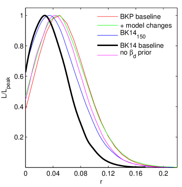
Fig. 5 shows one additional variation. It turns out that the tight prior on from Planck analysis of other regions of sky is becoming unnecessary. Removing the prior the peak position of the likelihood on shifts up slightly and broadens so that & (95%), while the likelihood curve for is close to Gaussian in shape with mean/ of 1.82/0.26. In Appendix E2 we investigate a variety of other variations from the baseline analysis and in Appendix E3 we perform some validation tests of the likelihood using simulations.
For the purposes of presentation we also run a likelihood analysis to find the CMB and foreground contributions on a bandpower-by-bandpower basis. The baseline analysis is a single fit to all 9 bandpowers across 66 spectra with 8 parameters. Instead we now perform 9 separate fits—one for each bandpower—across the 66 spectra, with 6 parameters in each fit. These 6 parameters are the amplitudes of CMB, dust and synchrotron plus , , and with identical priors to the baseline analysis. The results are shown in Fig. 6—the resulting CMB bandpowers are consistent with lensed-CDM while the dust bandpowers are consistent with the level of dust found in the baseline analysis. Synchrotron is tightly limited in all the bandpowers.

Conclusions.—As shown above, the BK14 data in combination with external maps produce -mode based constraints on the tensor-to-scalar ratio which place an upper limit at 95% confidence. The analysis of Planck full mission data in conjunction with external data produces the constraint () at 95% confidence (“Planck +lowP+lensing+ext” in Equation 39b of Ref. Planck Collaboration 2015 XIII (2015)), and are saturated at cosmic variance limits. The BK14 result constitutes the first -mode constraints that clearly surpass those from temperature anisotropies. In Fig. 7 we reproduce Ref. Planck Collaboration 2015 XIII (2015)’s result in the vs. plane, and show the effect of adding in our BK14 -mode data. The allowed region tightens and the joint result is (95%), although as emphasized in Ref. Planck Collaboration 2015 XIII (2015) the derived constraints on are more model dependent than ones.
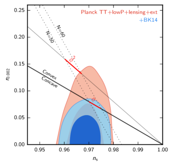
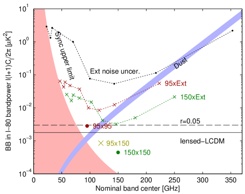
Fig. 8 compares signal levels and current noise uncertainties in the critical bandpower (updated from Fig. 13 of BKP). A second season of 95 GHz Keck Array data has already been recorded (in 2015) and will push the point down by a factor of 2. During 2015 two receivers were also operated in a third band centered on 220 GHz, producing deep maps which will improve dust separation. This 2015 data is under analysis and will be reported on in a future paper. In addition, BICEP3 began operations in 2015 in the 95 GHz band.
In this paper, we have presented an analysis of all BICEP2/Keck data up through the 2014 season, adding, for the first time, 95 GHz data from the Keck Array. We have updated our multi-frequency likelihood analysis with a more extensive foreground parameterization and the inclusion of external data from the 23 & 33 GHz bands of WMAP, in addition to all seven polarized bands of Planck. The baseline analysis yields and at 95% confidence, constraints that are robust to the variations explored in analysis and priors. With this result, -modes now offer the most powerful limits on inflationary gravitational waves, surpassing constraints from temperature anisotropies and other evidence for the first time. With upcoming multifrequency data the -mode constraints can be expected to steadily improve.
Acknowledgements.
The Keck Array project has been made possible through support from the National Science Foundation under Grants ANT-1145172 (Harvard), ANT-1145143 (Minnesota) & ANT-1145248 (Stanford), and from the Keck Foundation (Caltech). The development of antenna-coupled detector technology was supported by the JPL Research and Technology Development Fund and Grants No. 06-ARPA206-0040 and 10-SAT10-0017 from the NASA APRA and SAT programs. The development and testing of focal planes were supported by the Gordon and Betty Moore Foundation at Caltech. Readout electronics were supported by a Canada Foundation for Innovation grant to UBC. The computations in this paper were run on the Odyssey cluster supported by the FAS Science Division Research Computing Group at Harvard University. The analysis effort at Stanford and SLAC is partially supported by the U.S. DoE Office of Science. We thank the staff of the U.S. Antarctic Program and in particular the South Pole Station without whose help this research would not have been possible. Most special thanks go to our heroic winter-overs Robert Schwarz and Steffen Richter. We thank all those who have contributed past efforts to the BICEP–Keck Array series of experiments, including the BICEP1 team. We also thank the Planck and WMAP teams for the use of their data.References
- Penzias and Wilson (1965) A. A. Penzias and R. W. Wilson, Astrophys. J. 142, 419 (1965).
- Planck Collaboration 2015 XIII (2015) Planck Collaboration 2015 XIII, ArXiv e-prints (2015), arXiv:1502.01589 .
- Kamionkowski and Kovetz (2015) M. Kamionkowski and E. D. Kovetz, ArXiv e-prints (2015), arXiv:1510.06042 .
- Guth et al. (2014) A. H. Guth, D. I. Kaiser, and Y. Nomura, Physics Letters B 733, 112 (2014), arXiv:1312.7619 .
- Ijjas et al. (2014) A. Ijjas, P. J. Steinhardt, and A. Loeb, ArXiv e-prints (2014), arXiv:1402.6980 .
- Kovac et al. (2002) J. M. Kovac, E. M. Leitch, C. Pryke, J. E. Carlstrom, N. W. Halverson, and W. L. Holzapfel, Nature 420, 772 (2002), astro-ph/0209478 .
- Polarbear Collaboration (2014) Polarbear Collaboration, Astrophys. J. 794, 171 (2014), arXiv:1403.2369 .
- Keisler et al. (2015) R. Keisler, S. Hoover, N. Harrington, J. W. Henning, P. A. R. Ade, K. A. Aird, J. E. Austermann, J. A. Beall, A. N. Bender, B. A. Benson, L. E. Bleem, J. E. Carlstrom, C. L. Chang, H. C. Chiang, H.-M. Cho, R. Citron, T. M. Crawford, A. T. Crites, T. de Haan, M. A. Dobbs, W. Everett, J. Gallicchio, J. Gao, E. M. George, A. Gilbert, N. W. Halverson, D. Hanson, G. C. Hilton, G. P. Holder, W. L. Holzapfel, Z. Hou, J. D. Hrubes, N. Huang, J. Hubmayr, K. D. Irwin, L. Knox, A. T. Lee, E. M. Leitch, D. Li, D. Luong-Van, D. P. Marrone, J. J. McMahon, J. Mehl, S. S. Meyer, L. Mocanu, T. Natoli, J. P. Nibarger, V. Novosad, S. Padin, C. Pryke, C. L. Reichardt, J. E. Ruhl, B. R. Saliwanchik, J. T. Sayre, K. K. Schaffer, E. Shirokoff, G. Smecher, A. A. Stark, K. T. Story, C. Tucker, K. Vanderlinde, J. D. Vieira, G. Wang, N. Whitehorn, V. Yefremenko, and O. Zahn, Astrophys. J. 807, 151 (2015), arXiv:1503.02315 .
- BICEP1 Collaboration (2014) BICEP1 Collaboration, Astrophys. J. 783, 67 (2014), arXiv:1310.1422 .
- BICEP2 Collaboration I (2014) BICEP2 Collaboration I, Physical Review Letters 112, 241101 (2014), arXiv:1403.3985 .
- Keck Array and BICEP2 Collaborations V (2015) Keck Array and BICEP2 Collaborations V, Astrophys. J. 811, 126 (2015), arXiv:1502.00643 .
- Planck Collaboration Int. XIX (2015) Planck Collaboration Int. XIX, Astron. Astrophys. 576, A104 (2015), arXiv:1405.0871 .
- Planck Collaboration Int. XXX (2014) Planck Collaboration Int. XXX, ArXiv e-prints (2014), arXiv:1409.5738 .
- Flauger et al. (2014) R. Flauger, J. C. Hill, and D. N. Spergel, J. Cosmol. Astropart. Phys. 8, 039 (2014), arXiv:1405.7351 .
- Mortonson and Seljak (2014) M. J. Mortonson and U. Seljak, J. Cosmol. Astropart. Phys. 10, 035 (2014), arXiv:1405.5857 .
- BICEP2/Keck and Planck Collaborations (2015) BICEP2/Keck and Planck Collaborations, Physical Review Letters 114, 101301 (2015), arXiv:1502.00612 .
- BICEP2 Collaboration II (2014) BICEP2 Collaboration II, Astrophys. J. 792, 62 (2014), arXiv:1403.4302 .
- BICEP2/Keck and Spider Collaborations (2015) BICEP2/Keck and Spider Collaborations, Astrophys. J. 812, 176 (2015), arXiv:1502.00619 [astro-ph.IM] .
- Note (1) Appendices are in Supplemental Material http://xxx.yyy which includes references (Choi and Page, 2015; Dunkley et al., 2009).
- Note (2) See http://www.cosmos.esa.int/web/planck/pla.
- Planck Collaboration 2015 I (2015) Planck Collaboration 2015 I, ArXiv e-prints (2015), arXiv:1502.01582 .
- Note (3) See http://lambda.gsfc.nasa.gov/product/map/dr5/m_products.cfm.
- Bennett et al. (2013) C. L. Bennett, D. Larson, J. L. Weiland, N. Jarosik, G. Hinshaw, N. Odegard, K. M. Smith, R. S. Hill, B. Gold, M. Halpern, E. Komatsu, M. R. Nolta, L. Page, D. N. Spergel, E. Wollack, J. Dunkley, A. Kogut, M. Limon, S. S. Meyer, G. S. Tucker, and E. L. Wright, Astrophys. J. Suppl. Ser. 208, 20 (2013), arXiv:1212.5225 .
- Planck Collaboration 2015 XII (2015) Planck Collaboration 2015 XII, ArXiv e-prints (2015), arXiv:1509.06348 .
- Hamimeche and Lewis (2008) S. Hamimeche and A. Lewis, Phys. Rev. D 77, 103013 (2008), arXiv:0801.0554 .
- Lewis and Bridle (2002) A. Lewis and S. Bridle, Phys. Rev. D66, 103511 (2002), astro-ph/0205436 .
- Planck Collaboration Int. XXII (2015) Planck Collaboration Int. XXII, Astron. Astrophys. 576, A107 (2015), arXiv:1405.0874 .
- Fuskeland et al. (2014) U. Fuskeland, I. K. Wehus, H. K. Eriksen, and S. K. Næss, Astrophys. J. 790, 104 (2014), arXiv:1404.5323 .
- Note (4) See http://lambda.gsfc.nasa.gov/product/map/dr5/mcmc_maps_info.cfm.
- Choi and Page (2015) S. K. Choi and L. A. Page, ArXiv e-prints (2015), arXiv:1509.05934 .
- Dunkley et al. (2009) J. Dunkley, A. Amblard, C. Baccigalupi, M. Betoule, D. Chuss, A. Cooray, J. Delabrouille, C. Dickinson, G. Dobler, J. Dotson, H. K. Eriksen, D. Finkbeiner, D. Fixsen, P. Fosalba, A. Fraisse, C. Hirata, A. Kogut, J. Kristiansen, C. Lawrence, A. M. Magalhães, M. A. Miville-Deschenes, et al., AIP Conf. Proc. 1141, 222 (2009), arXiv:0811.3915 .
Appendix A Maps
Figures 9 & 10 show the full sets of // maps at 150 & 95 GHz. The right side of each figure shows realizations of noise created by randomly flipping the sign of data subsets while coadding the map—see Sec. V.B of BK-I for further details.
Appendix B Keck Array 95 GHz Power Spectra and Internal Consistency Tests
A powerful internal consistency test are data split difference tests which we refer to as “jackknifes”. As well as the full coadd signal maps we also form many pairs of split maps where the splits are chosen such that one might expect different systematic contamination in the two halves of the split. The split halves are differenced and the power spectra taken. We then take the deviations of these from the mean of signal+noise simulations and form and (sum of deviations) statistics. In this section we perform tests of the new 95 GHz data set which are exactly analogous to the tests of the previous 150 GHz data sets performed in Sec. VII.C of BK-I and Sec. 6.3 of BK-V. Fig. 11 shows the signal spectra and a sample set of jackknife spectra. All the signal spectra are consistent with lensed-CDM and the jackknife spectra with null.
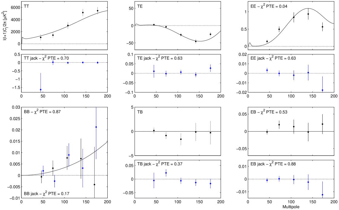
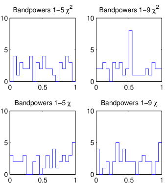
Table B shows the and statistics for the full set of 95 GHz jackknife tests and Fig. 12 presents the same results in graphical form. Note that these values are partially correlated—particularly the 1–5 and 1–9 versions of each statistic. We conclude that there is no evidence for corruption of the data at a level exceeding the noise.
| Jackknife | Band powers | Band powers | Band powers | Band powers |
|---|---|---|---|---|
| 1–5 | 1–9 | 1–5 | 1–9 | |
| Deck jackknife | ||||
| EE | 0.625 | 0.591 | 0.523 | 0.569 |
| BB | 0.166 | 0.192 | 0.076 | 0.020 |
| EB | 0.876 | 0.539 | 0.814 | 0.445 |
| Scan Dir jackknife | ||||
| EE | 0.439 | 0.513 | 0.760 | 0.423 |
| BB | 0.944 | 0.535 | 0.565 | 0.168 |
| EB | 0.539 | 0.192 | 0.912 | 0.980 |
| Tag Split jackknife | ||||
| EE | 0.543 | 0.537 | 0.810 | 0.938 |
| BB | 0.768 | 0.780 | 0.687 | 0.539 |
| EB | 0.313 | 0.547 | 0.407 | 0.451 |
| Tile jackknife | ||||
| EE | 0.234 | 0.477 | 0.395 | 0.709 |
| BB | 0.050 | 0.072 | 0.012 | 0.046 |
| EB | 0.828 | 0.902 | 0.812 | 0.822 |
| Phase jackknife | ||||
| EE | 0.862 | 0.982 | 0.577 | 0.471 |
| BB | 0.944 | 0.521 | 0.639 | 0.325 |
| EB | 0.691 | 0.890 | 0.204 | 0.357 |
| Mux Col jackknife | ||||
| EE | 0.084 | 0.146 | 0.182 | 0.337 |
| BB | 0.172 | 0.337 | 0.012 | 0.152 |
| EB | 0.541 | 0.695 | 0.956 | 0.812 |
| Alt Deck jackknife | ||||
| EE | 0.098 | 0.076 | 0.030 | 0.036 |
| BB | 0.092 | 0.126 | 0.102 | 0.140 |
| EB | 0.858 | 0.842 | 0.858 | 0.741 |
| Mux Row jackknife | ||||
| EE | 0.232 | 0.289 | 0.699 | 0.918 |
| BB | 0.289 | 0.267 | 0.082 | 0.014 |
| EB | 0.148 | 0.130 | 0.996 | 0.998 |
| Tile/Deck jackknife | ||||
| EE | 0.924 | 0.956 | 0.162 | 0.399 |
| BB | 0.507 | 0.034 | 0.561 | 0.343 |
| EB | 0.477 | 0.361 | 0.954 | 0.994 |
| Focal Plane inner/outer jackknife | ||||
| EE | 0.477 | 0.335 | 0.200 | 0.792 |
| BB | 0.886 | 0.437 | 0.762 | 0.569 |
| EB | 0.595 | 0.876 | 0.926 | 0.780 |
| Tile top/bottom jackknife | ||||
| EE | 0.261 | 0.519 | 0.998 | 0.990 |
| BB | 0.756 | 0.890 | 0.415 | 0.431 |
| EB | 0.850 | 0.920 | 0.377 | 0.317 |
| Tile inner/outer jackknife | ||||
| EE | 0.184 | 0.353 | 0.427 | 0.529 |
| BB | 0.772 | 0.772 | 0.749 | 0.707 |
| EB | 0.407 | 0.038 | 0.934 | 0.667 |
| Moon jackknife | ||||
| EE | 0.569 | 0.701 | 0.228 | 0.251 |
| BB | 0.305 | 0.465 | 0.978 | 0.990 |
| EB | 0.349 | 0.507 | 0.677 | 0.301 |
| A/B offset best/worst | ||||
| EE | 0.635 | 0.267 | 0.104 | 0.431 |
| BB | 0.407 | 0.387 | 0.677 | 0.287 |
| EB | 0.321 | 0.605 | 0.860 | 0.685 |
Appendix C 150 GHz Spectral Stability
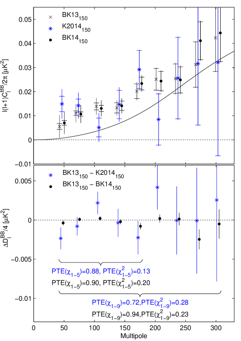
Questions were raised as to whether the BICEP2 and Keck Array 2012+2013 spectra are mutually compatible. We investigated this in Sec. 8 of BK-V and concluded that they are. Here we perform a similar test on the difference of the BK13150 and BK14150 spectra—i.e. when adding the additional 150 GHz data from 2014. We compare the differences of the real spectra to the differences of simulations which share the same underlying input skies. Fig. 13 shows the results. While the bandpowers do shift around even when adding only % of additional data these shifts are seen to be consistent with noise fluctuation. We go on to perform one more test—we instead take the difference of the BK13150 and the 2014 only 150 GHz spectrum (which we refer to as K2014150). Since we are measuring the bandpower differences in units of the expected shift given the degree of common data we expect, and find, similar results.
Appendix D Additional Spectra
Figures 2 & 3 show only a small subset of the spectra which are used in the likelihood analysis and included in the COSMOMC input file. We are using two BICEP2/Keck bands, two WMAP bands, and seven Planck bands resulting in 11 auto and 55 cross-spectra. In Fig. 14 we show all of these together with the baseline lensed-CDM+dust and upper limit lensed-CDM+synchrotron models. Note that, as expected from Fig. 8, several spectra contribute to constraining synchrotron.
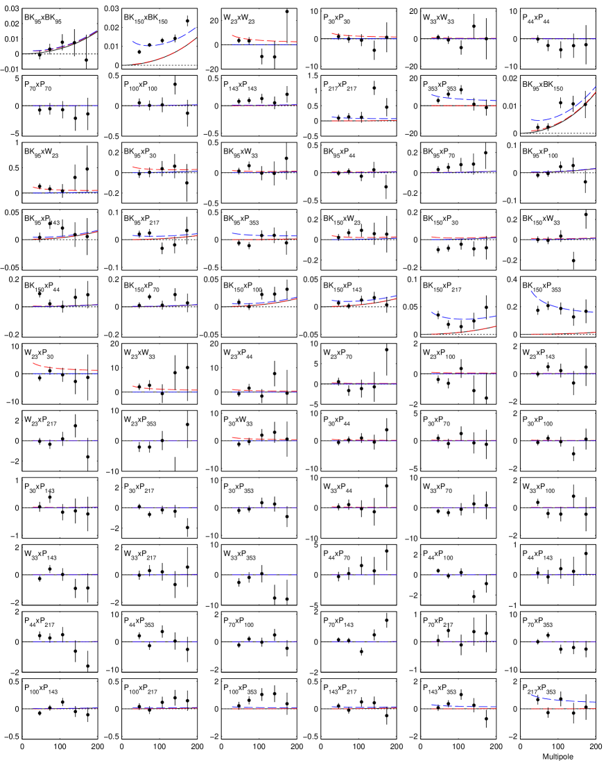
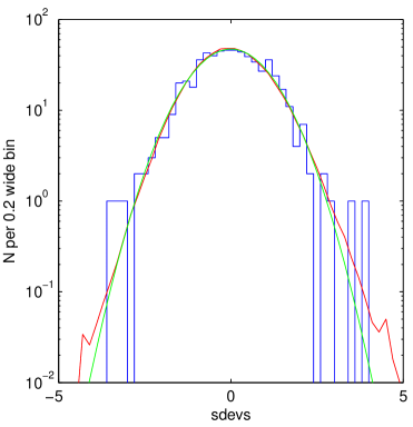
Fig. 15 shows the distribution of the normalized deviations between the data and the maximum likelihood (ML) model (i.e. data minus expectation value divided by the square root of the diagonal of the bandpower covariance matrix). Since the bandpower distributions are not strictly Gaussian we overplot the same quantity from a set of lensed-CDM+dust+noise simulations evaluated against their input model. (These simulations use the model K2, and .) We see one nominally point which is bandpower four of PP217 (see Fig. 14)—comparing to the simulated distribution this event it not unlikely. Taking versus the ML model yields 654, which compared to the distribution from simulations has a PTE of . We conclude that there is no evidence that the signal or noise models are an inadequate explanation of the data.
Appendix E Likelihood Variation and Validation
E.1 Likelihood Evolution
In Fig. 5 some evolutionary steps were shown between the previous BKP analysis and the new BK14 analysis presented in this paper. Fig 16 shows some additional detail. The first step is to the alternate analysis including synchrotron which was shown in Fig. 8 of BKP (solid red to dashed-red). This used the BK13 maps plus all of the polarized bands of Planck and set and . (In BKP the synchrotron pivot frequency was set to 150 GHz but since a fixed value of was used there we can simply transform the results to the pivot of 23 GHz used in this work.) Next we show the cumulative effects of model changes which we have made for this paper:
We extend the bandpower range from five () to nine () bandpowers—given that lensing is included in the model there is no real reason not to include these additional bandpowers (dashed-red to solid blue). We see that the constraint tightens somewhat.
We switch from the use of Planck single-frequency split/split cross-spectra (in this case Y1Y2) to full map auto spectra (blue to cyan). This is done for technical reasons—substituting in the cross-spectra causes numerical problems in the HL likelihood. The auto spectra have higher signal-to-noise and the constraint on tightens further.
We include the WMAP 23 & 33 GHz bands and see that these have considerable additional power to constrain synchrotron (cyan to magenta).
In BKP we used as this is the mean value within our field of the “model f” synchrotron spectral index maps available for download from the WMAP website 333See http://lambda.gsfc.nasa.gov/product/map/dr5/mcmc_maps_info.cfm. However that analysis does not distinguish between the spectral behavior of temperature and polarization anisotropy. Ref. Fuskeland et al. (2014) analyzed the WMAP data and found a mean value of for polarization at high galactic latitude. In this analysis we use a central value of , and since possible patch-to-patch variation is poorly constrained, to be conservative we marginalize over a Gaussian prior with width . More recently Ref. Choi and Page (2015) examined the same data and found with considerable fluctuation. This change has very little effect (magenta to yellow).
Polarized synchrotron and dust emission can be spatially correlated—indeed they are guaranteed to be so on the largest scales. Ref. Choi and Page (2015) reports a correlation of 0.2 for . To be conservative in this analysis we marginalize over the range . This causes the constraint on synchrotron to tighten because of the non-detection of signal in spectra like PP353 (yellow to green). We note that the data prefer the value as seen in the upper-right panel of Fig. 4.
In BKP we used following the analysis of large regions of high latitude sky in Ref. Planck Collaboration Int. XXX (2014), and taken from Ref. Dunkley et al. (2009). In this work we found that we can marginalize over generous ranges in these parameters & with only a tiny change in the bottom line results so we choose to do so (green to dashed-blue).
Finally we show the changes resulting from adding the new 150 GHz and 95 GHz data (dashed-blue to dashed-black and dashed-black to heavy-black). As already seen in Fig. 5 these are much more significant.
E.2 Likelihood Variation
In Fig. 17 we investigate several variations to the baseline analysis in terms of the model priors and input data sets. The first four of these loosen the priors and/or remove data, while the final three tighten the priors and/or add data.

First we repeat a variation already shown in Fig. 5—we remove the prior on the frequency spectral index of dust (black to cyan). The data then constrains to a well behaved, approximately Gaussian range (not shown) with mean/ of 1.82/0.26. The value of shifts up slightly but, with the steeper slope versus frequency, the constraint also shifts up slightly to with a zero-to-peak likelihood ratio of 0.44 (10% likely if ).
Second we relax the prior on the frequency spectral index of synchrotron to and see that this has very little effect on any of the curves (black to green).
Third we remove all the Planck LFI bands from consideration (black to magenta). This causes the peak of the constraint to shift down a little and the constraint to peak quite strongly away from zero, while the constraint is not significantly affected.
Fourth we drop the two bands of WMAP (black to yellow). This slightly decreases the zero-to-peak ratio of the constraint and significantly tightens the constraint.
We now progressively tighten the priors. For the fifth curve we switch from to the value preferred by Ref. Choi and Page (2015) (black to dashed-red). This makes almost no difference to any of the constraints, although we do note that the up-tick in the curve approaching zero goes away.
In the sixth curve we also go back to the tight priors and which were used in the BKP analysis (dashed-red to blue). As expected from Fig. 16 this makes almost no difference to any of the constraints.
Finally in the seventh curve we also include all the and spectra under the assumption that the ratios for dust and synchrotron are exactly 2 (blue to dashed-black). For dust this ratio was found to apply when averaging over large areas of sky in Ref. Planck Collaboration Int. XXX (2014). Ref. Choi and Page (2015) states that this ratio also applies on average for synchrotron. Assuming this fixed ratio leads to extra constraining power—the curve shifts up slightly, the curve narrows and the curve peaks strongly away from zero. It is unclear how much patch-to-patch variation we should in fact allow in the ratio so this variation should not be over interpreted at this time.
E.3 Likelihood Validation
As already mentioned we run full timestream simulations of a lensed-CDM+dust model ( K2, and ). We would like to check that the HL likelihood as implemented is capable of recovering the input values of this model. However if we run the standard COSMOMC analysis on these we of course find that the ML values are biased, since only zero or positive values of and are allowed. We therefore instead run a ML search on each sim realization where the values of and are artificially allowed to go negative (as is although in practice it doesn’t). Fig. 18 shows the results—the input values are recovered in the mean as expected.
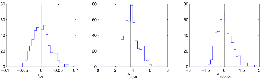
An additional piece of information which comes from this study is the standard deviation of the recovered ML parameter, . Unlike the width of the 68% highest posterior density intervals derived from the marginalized curve shown in Fig. 4 and quoted with our baseline results, this statistic is insensitive to where the peak value preferred by the data happens to lie, and is therefore a more robust measure of the intrinsic constraining power of the experimental data.