On the Alignment Limit of the NMSSM Higgs Sector

Abstract

The Next-to-Minimal Supersymmetric extension of the Standard Model (NMSSM) with a Higgs boson of mass 125 GeV can be compatible with stop masses of order of the electroweak scale, thereby reducing the degree of fine-tuning necessary to achieve electroweak symmetry breaking. Moreover, in an attractive region of the NMSSM parameter space, corresponding to the “alignment limit” in which one of the neutral Higgs fields lies approximately in the same direction in field space as the doublet Higgs vacuum expectation value, the observed Higgs boson is predicted to have Standard-Model-like properties. We derive analytical expressions for the alignment conditions and show that they point toward a more natural region of parameter space for electroweak symmetry breaking, while allowing for perturbativity of the theory up to the Planck scale. Moreover, the alignment limit in the NMSSM leads to a well defined spectrum in the Higgs and Higgsino sectors, and yields a rich and interesting Higgs boson phenomenology that can be tested at the LHC. We discuss the most promising channels for discovery and present several benchmark points for further study.

I Introduction

The recent discovery of a scalar resonance Aad:2012tfa ; Chatrchyan:2012ufa , with properties similar to the Higgs boson of the Standard Model (SM) motivates the study of models of electroweak symmetry breaking which are weakly coupled at the weak scale. Low energy supersymmetric theories with flavor independent mass parameters are particularly well motivated models of this class, in which electroweak symmetry breaking is triggered by radiative corrections of the Higgs mass parameters induced by supersymmetry breaking effects in the top-quark sector.

The Higgs sector of the Minimal Supersymmetric extension of the Standard Model (MSSM) is a two-Higgs-doublet model (2HDM) in which the tree-level mass of the CP-even Higgs boson associated with electroweak symmetry breaking is bounded from above by the $Z$ boson mass, $m_{Z}$. Consistency with the observed Higgs mass may be obtained by means of large radiative corrections, which depend logarithmically on the scalar-top quark (stop) masses, and on the stop mixing mass parameters in a quadratic and quartic fashion mssmhiggsradcorr –Lee:2015uza . The large values of the stop mass parameters and mixings necessary to obtain the proper Higgs mass also lead to large negative corrections to the Higgs mass parameter that in general must be canceled by an appropriate choice of the supersymmetric Higgsino mass parameter $\mu$ in order to obtain the proper electroweak symmetry breaking scale. For large stop masses, such a cancelation is unnatural in the absence of specific correlations among the supersymmetry breaking parameters (whose origins are presently unknown).

The Next-to-Minimal Supersymmetric extension of the Standard Model (NMSSM) Ellwanger:2009dp shares many properties with the MSSM, but the Higgs sector is extended by the addition of a singlet superfield, leading to two additional neutral Higgs bosons. The tree-level Higgs mass receives additional contributions proportional to the square of the superpotential coupling $\lambda$ between the singlet and the doublet Higgs sectors and thus is no longer bounded from above by $m_{Z}$. Such contributions become negligible for large values of $\tan\beta$, the ratio of the two Higgs doublet vacuum expectation values (VEVs). Therefore, for sizable values of $\lambda$ and values of $\tan\beta$ of order one, an observationally consistent Higgs mass may be obtained without the need for large radiative corrections, enabling a more natural breaking of the electroweak symmetry than in the MSSM.

The SM-like properties of the 125 GeV Higgs boson in both the MSSM and the NMSSM may be ensured via the decoupling limit, where all the Higgs bosons (excluding the observed Higgs boson with a mass of 125 GeV) are much heavier than the electroweak scale. However, the decoupling limit is not the only way to achieve a SM-like Higgs boson, as observed in Ref. Gunion:2002zf and rediscovered recently in Refs. Delgado:2013zfa ; Craig:2013hca ; whitepaper ; Carena:2013ooa ; Haber:2013mia : a SM-like Higgs can be obtained by way of the “alignment limit,” where one of the neutral Higgs mass eigenstates is approximately aligned in field space with the Higgs doublet VEV. Subsequent studies have continued to focus on the alignment limit in 2HDMs Carena:2014nza ; Dev:2014yca . In particular, approximate alignment may be obtained in the MSSM for moderate to large values of $\tan\beta$ and for large values of the ratio $\mu A_{t}/M_{S}^{2}$, where $A_{t}$ is the stop mixing mass parameter, $\mu$ is the supersymmetric Higgsino mass parameter, and $M_{S}^{2}$ is the average of the two stop squared-masses Carena:2013ooa . Moreover, there is an interesting complementarity between precision measurements of the SM-like Higgs properties and direct searches for non-standard Higgs bosons in the MSSM Carena:2014nza .

In this work we extend the study of alignment without decoupling beyond the 2HDM to the NMSSM where there is an additional singlet scalar as well as the two doublet scalars. In fact, it will become clear that our analysis is quite general and can be applied even beyond the NMSSM. We demonstrate that the alignment conditions in the NMSSM Higgs sector are fulfilled in regions of parameters space consistent with a natural breaking of the electroweak symmetry, where the stop mass parameters are of the order of the electroweak scale. Moreover, under the assumption that all couplings remain perturbative up to the Planck scale, we show that the requirements of natural electroweak symmetry breaking and the alignment limit in the Higgs sector lead to well defined spectra for Higgs bosons and Higgsinos that may be tested experimentally in the near future at the LHC.

There have been several recent works analyzing similar questions in the NMSSM after the discovery of the Higgs boson (for example, see Refs. Ellwanger:2011aa –King:2014xwa ). In particular, in Ref. King:2014xwa a numerical scan over the NMSSM parameter space was employed to determine the regions of the NMSSM parameter space that are consistent with present Higgs boson precision measurements and searches for other Higgs boson states and supersymmetric particles. These parameter regions include those that are consistent with the alignment conditions examined in this paper. Consequently, the benchmark scenarios presented in Ref. King:2014xwa exhibit similar features to the ones presented in Appendix D of this work. In contrast to previous studies, in this paper we develop an analytic understanding of the alignment conditions that lead to consistency with the observed Higgs physics, and we present a detailed phenomenological study of the non-SM-like Higgs boson couplings to fermions and gauge bosons.

This paper is organized as follows. In section II, we analyze the alignment conditions in extensions of the Higgs sector with two doublets and one singlet, and discuss the NMSSM as a particular example. In section III, we examine the associated Higgs phenomenology. In section IV, we study the Higgs production and decay modes relevant for run 2 of the LHC, and we present our conclusions in section V. In Appendix A, details of the scalar potential in the Higgs basis for the two doublets/one singlet model are given, along with the corresponding expressions for the NMSSM Higgs sector. Explicit expressions for the rotation matrix elements relating the Higgs basis and mass eigenbasis are provided in Appendix B. In Appendix C, we exhibit the trilinear scalar self-couplings and the couplings of the neutral scalars to the $Z$ boson. Finally, in Appendix D we present several NMSSM benchmark scenarios that illustrate features of the Higgs phenomenology considered in this paper.

II NMSSM Alignment Conditions

II.1 Generalities

The scalar sector of the NMSSM consists of two electroweak doublets and one electroweak singlet. We first present some general considerations of the “alignment limit” in the Higgs sector that can be applied broadly to any Higgs sector made up of two doublets and one singlet. Similar to the case of the 2HDM, the discussion is most transparent when one adopts the Higgs basis higgsbasis ; Branco:1999fs , in which only the neutral component of one of the two doublet scalars acquires a non-zero VEV.

In the paradigm of spontaneous electroweak symmetry breaking, a tree-level scalar coupling to massive electroweak gauge bosons is directly proportional to the strength of the VEV residing in any scalar with non-trivial SU(2)${}_{L}\times$U(1)_Y quantum numbers. Thus, in the Higgs basis, if the scalar doublet Higgs field with the nonzero VEV coincides with one of the scalar mass eigenstates (the so-called alignment limit), then this state couples to $W$ and $Z$ bosons with full SM strength and is the natural candidate to be the SM-like 125 GeV Higgs boson. Non-zero couplings of the other mass eigenstates to the massive gauge bosons arise only away from the alignment limit.

In the Higgs basis, we define the hypercharge-one doublet fields $H_{1}$ and $H_{2}$ such that the VEVs of the corresponding neutral components are given by

$$\langle H^{0}_{1}\rangle=\frac{v}{\sqrt{2}}\,,\qquad\quad\langle H^{0}_{2}\rangle=0\,,$$ (1)

where $v\simeq 246$ GeV. The singlet scalar field $S$ also possesses a non-zero VEV,

$$\langle S\rangle\equiv v_{s}\,.$$ (2)

We shall make the simplifying assumption that the scalar potential preserves CP, which is not spontaneously broken in the vacuum. Thus, the phases of the Higgs fields can be chosen such that $v_{s}$ is real. We then define the following neutral scalar fields,

$$H^{\rm SM} \equiv \sqrt{2}\,{\rm Re}~{}H_{1}^{0}-v\,,\qquad\quad H^{\rm NSM}\equiv\sqrt{2}\,{\rm Re}~{}H_{2}^{0}\,,\qquad H^{\rm S}\equiv\sqrt{2}\,({\rm Re}~{}S-v_{s})\,,$$ (3)

$$A^{\rm SM} \equiv \sqrt{2}\,{\rm Im}~{}H_{1}^{0}\,,\qquad\qquad\quad A^{\rm NSM}\equiv\sqrt{2}\,{\rm Im}~{}H_{2}^{0}\,,\qquad A^{\rm S}\equiv\sqrt{2}\,{\rm Im}~{}S\,,$$ (4)

where $A^{\rm SM}$ is the Goldstone field that is absorbed by the $Z$ and provides its longitudinal degree of freedom. Under the assumption of CP conservation, the scalar fields $H^{\rm SM}$, $H^{\rm NSM}$ and $H^{\rm S}$ mix to yield three neutral CP-even scalar mass eigenstates of the following real symmetric squared-mass matrix,

$$\mathcal{M}_{S}^{2}=\left(\begin{array}[]{ccc}\mathcal{M}^{2}_{11}&\mathcal{M}^{2}_{12}&\mathcal{M}^{2}_{13}\\ \mathcal{M}^{2}_{12}&\mathcal{M}^{2}_{22}&\mathcal{M}^{2}_{23}\\ \mathcal{M}^{2}_{13}&\mathcal{M}^{2}_{23}&\mathcal{M}^{2}_{33}\end{array}\right)\ ,$$ (5)

The exact alignment limit is realized when the following two conditions are satisfied

$$\mathcal{M}^{2}_{12}=0\ ,\qquad\mathcal{M}^{2}_{13}=0\ .$$ (6)

In this case, $H^{\rm SM}$ is a CP-even mass-eigenstate scalar with squared mass $\mathcal{M}^{2}_{11}$, and its couplings to massive gauge bosons and fermions are precisely those of the SM Higgs boson. In practice, we only need to require that the observed 125 GeV scalar (henceforth denoted by $h$) is SM-like, which implies that the alignment limit is approximately realized. In this case, Eq. (6) is replaced by the following conditions:

$$\mathcal{M}^{2}_{12}\ll\mathcal{O}(v^{2})\ ,\qquad\quad\mathcal{M}^{2}_{13}\ll\mathcal{O}(v^{2})\ ,$$ (7)

which imply that

$$m_{h}^{2}\simeq\mathcal{M}^{2}_{11}=(125~{}{\rm GeV})^{2}\,.$$ (8)

Corrections to Eq. (8) appear only at second order in the perturbative expansion and thus are proportional to the squares of $\mathcal{M}^{2}_{12}$ or $\mathcal{M}^{2}_{13}$, respectively.

We shall denote the CP-even Higgs mass-eigenstate fields by $h$, $H$, and $h_{S}$, where $h$ is identified with the observed SM-like Higgs boson, $H$ is a dominantly doublet scalar field and $h_{S}$ is a dominantly singlet scalar field. The mass-eigenstate fields $\{h,H,h_{S}\}$ are related to $\{H^{\rm SM},H^{\rm NSM},H^{\rm S}\}$ by a real orthogonal matrix $\mathcal{R}$,

$$\begin{pmatrix}h\\ H\\ h_{S}\end{pmatrix}=\mathcal{R}\begin{pmatrix}\phantom{-}H^{\rm SM}\\ H^{\rm NSM}\\ \phantom{-}H^{\rm S}\end{pmatrix}\,,$$ (9)

where

$$\mathcal{R}=R_{23}^{\prime}R_{13}R_{12} = \left(\begin{array}[]{ccc}1&\phantom{-}0&\phantom{-}0\\ 0&\,\,\,\,-c_{23}\phantom{-}&-s_{23}\\ 0&-s_{23}&\phantom{-}c_{23}\end{array}\right)\left(\begin{array}[]{ccc}\phantom{-}c_{13}&\phantom{-}0&\phantom{-}s_{13}\\ \phantom{-}0&\phantom{-}1&\phantom{-}0\\ -s_{13}&\phantom{-}0&\phantom{-}c_{13}\end{array}\right)\left(\begin{array}[]{ccc}\phantom{-}c_{12}&\phantom{-}s_{12}&\phantom{-}0\\ -s_{12}&\phantom{-}c_{12}&\phantom{-}0\\ \phantom{-}0&\phantom{-}0&\phantom{-}1\end{array}\right)$$ (19)

$$= \left(\begin{array}[]{ccc}c_{13}c_{12}&\quad c_{13}s_{12}&\quad s_{13}\\[6.0pt] c_{23}s_{12}+c_{12}s_{13}s_{23}&\quad-c_{12}c_{23}+s_{12}s_{13}s_{23}&\quad-c_{13}s_{23}\\[6.0pt] -c_{12}c_{23}s_{13}+s_{12}s_{23}&\quad-c_{23}s_{12}s_{13}-c_{12}s_{23}&\quad\phantom{-}c_{13}c_{23}\end{array}\right)\,,$$ (23)

where $c_{ij}\equiv\cos\theta_{ij}$ and $s_{ij}\equiv\sin\theta_{ij}$. The mixing angles $\theta_{ij}$ are defined modulo $\pi$. It is convenient to choose $|\theta_{ij}|\leq\tfrac{1}{2}\pi$, in which case $c_{ij}\geq 0$. The mixing angles $\theta_{ij}$ are determined by the diagonalization equation,

$$\mathcal{R}~{}\mathcal{M}^{2}_{S}~{}\mathcal{R}^{T}={\rm diag}(m_{h}^{2},m_{H}^{2},m_{h_{S}}^{2})\,.$$ (24)

We can use Eqs. (19) and (24) to obtain exact expressions for the mixing angles in terms of $m^{2}_{h}$ and the elements of $\mathcal{M}^{2}_{S}$ as follows. Multiply Eq. (24) on the left by $\mathcal{R}^{T}$ and consider the first column of the resulting matrix equation. This yields three equations, which can be rearranged into the following form,

$$x\mathcal{M}^{2}_{12}+y\mathcal{M}^{2}_{13} = m_{h}^{2}-\mathcal{M}^{2}_{11}\,,$$ (25)

$$x\mathcal{M}^{2}_{23}+\mathcal{M}^{2}_{13} = y\bigl{(}m_{h}^{2}-\mathcal{M}^{2}_{33}\bigr{)}\,,$$ (26)

$$y\mathcal{M}^{2}_{23}+\mathcal{M}^{2}_{12} = x\bigl{(}m_{h}^{2}-\mathcal{M}^{2}_{22}\bigr{)}\,,$$ (27)

where $x\equiv s_{12}/c_{12}$ and $y\equiv s_{13}/(c_{12}c_{13})$ and correspond to the ratios of the NSM and S components to the SM component of $h$, respectively. Eliminating $y$ from Eqs. (26) and (27) yields an expression for $x$. To obtain the corresponding expression for $y$, it is more convenient to return to Eqs. (26) and (27) and eliminate $x$. The resulting expressions are:

$$x\equiv\frac{s_{12}}{c_{12}} = \frac{\mathcal{M}^{2}_{13}\mathcal{M}^{2}_{23}-\mathcal{M}^{2}_{12}\bigl{(}\mathcal{M}^{2}_{33}-m_{h}^{2}\bigr{)}}{\bigl{(}\mathcal{M}^{2}_{22}-m_{h}^{2}\bigr{)}\bigl{(}\mathcal{M}^{2}_{33}-m_{h}^{2}\bigr{)}-\mathcal{M}^{4}_{23}}\,,$$ (28)

$$y\equiv\frac{s_{13}}{c_{12}c_{13}} = \frac{\mathcal{M}^{2}_{12}\mathcal{M}^{2}_{23}-\mathcal{M}^{2}_{13}\bigl{(}\mathcal{M}^{2}_{22}-m_{h}^{2}\bigr{)}}{\bigl{(}\mathcal{M}^{2}_{22}-m_{h}^{2}\bigr{)}\bigl{(}\mathcal{M}^{2}_{33}-m_{h}^{2}\bigr{)}-\mathcal{M}^{4}_{23}}\,,$$ (29)

which are equivalent to Eqs. (142) and (143) of Appendix B. Inserting the above results for $x$ and $y$ back into Eq. (25) then yields a cubic polynomial equation for $m_{h}^{2}$, which we recognize as the characteristic equation obtained by solving the eigenvalue problem for $\mathcal{M}_{S}^{2}$. The approximate alignment conditions given in Eq. (7) imply that $|s_{12}|\ll 1$ and $|s_{13}|\ll 1$, in which case one can approximate $m_{h}^{2}\simeq\mathcal{M}^{2}_{11}$ in Eqs. (28) and (29) to very good accuracy.

Likewise, repeating the above exercise for $H$, we can obtain the ratio of the S component to the NSM component of $H$ [cf. Eq. (145)],

$$\frac{c_{13}s_{23}}{c_{12}c_{23}-s_{12}s_{13}s_{23}}=\frac{\mathcal{M}_{23}^{2}(\mathcal{M}_{11}^{2}-m_{H}^{2})-\mathcal{M}_{12}^{2}\mathcal{M}_{13}^{2}}{\mathcal{M}_{23}^{4}+(\mathcal{M}_{11}^{2}-m_{H}^{2})(m_{H}^{2}-\mathcal{M}_{33}^{2})}\,.$$ (30)

In the exact alignment limit where $\mathcal{M}_{12}^{2}=\mathcal{M}_{13}^{2}=0$ (and hence $s_{12}=s_{13}=0$), and when $\mathcal{M}_{23}^{2}\ll m_{H}^{2}$, Eq. (30) reduces to

$$\frac{s_{23}}{c_{23}}=\frac{\mathcal{M}_{23}^{2}}{m_{H}^{2}-\mathcal{M}_{33}^{2}}\,.$$ (31)

Our choice of $\det\mathcal{R}=-1$ in Eq. (9) requires an explanation. In the limit where there is no mixing of $H^{\rm S}$ with the Higgs doublet fields $H^{\rm SM}$ and $H^{\rm NSM}$, we have $s_{13}=s_{23}=0$ (and $c_{13}=c_{23}=1$ by convention), which yields 

$$h=c_{12}H^{\rm SM}+s_{12}H^{\rm NSM}\,,\qquad H=s_{12}H^{\rm SM}-c_{12}H^{\rm NSM}\,.$$ (32)

The transformation from $\{H^{\rm SM},H^{\rm NSM}\}$ to $\{h,H\}$ given in Eq. (32) employs a $2\times 2$ orthogonal matrix of determinant $-1$. Indeed, in the standard conventions of the 2HDM literature (see Refs. Gunion:1989we ; Branco:2011iw for reviews), we identify $c_{12}=\sin(\beta-\alpha)$ and $s_{12}=\cos(\beta-\alpha)$.

We next turn to the Higgs couplings to vector bosons and fermions. The interaction of a neutral Higgs field with a pair of massive gauge bosons $VV=W^{+}W^{-}$ or $ZZ$ arises from scalar field kinetic energy terms after replacing an ordinary derivative with a covariant derivative when acting on the electroweak doublet scalars. After spontaneous symmetry breaking, only the interaction term $H^{\rm SM}VV$ is generated. Using Eq. (9),

$$H^{\rm SM}=\mathcal{R}_{11}h+\mathcal{R}_{21}H+\mathcal{R}_{31}h_{S}\,,$$ (33)

which then yields the following couplings normalized to the corresponding SM values,

$$g_{hVV} = \mathcal{R}_{11}=c_{13}c_{12}\,,$$ (34)

$$g_{HVV} = \mathcal{R}_{21}=c_{23}s_{12}+c_{12}s_{13}s_{23}\,,$$ (35)

$$g_{h_{S}VV} = \mathcal{R}_{31}=-c_{12}c_{23}s_{13}+s_{12}s_{23}\,.$$ (36)

Note that in the limit where there is no mixing of $H^{\rm S}$ with the Higgs doublet fields $H^{\rm SM}$ and $H^{\rm NSM}$, we recover the standard 2HDM expressions $g_{hVV}=\sin(\beta-\alpha)$ and $g_{HVV}=\cos(\beta-\alpha)$.

For the Higgs interactions with the fermions, we employ the so-called Type-II Higgs-fermion Yukawa couplings Hall:1981bc as mandated by the holomorphic superpotential mssmhiggs ; Gunion:1984yn ,

$$-\mathscr{L}_{\rm Yuk}=\epsilon_{ij}\bigl{[}h_{b}\overline{b}_{R}H_{d}^{i}Q^{j}_{L}+h_{t}\overline{t}_{R}Q^{i}_{L}H_{u}^{j}\bigr{]}+{\rm h.c.}\,,$$ (37)

where $Q_{L}=(u,d)$. The scalar doublet fields $H_{d}$ and $H_{u}$ have hypercharges $-1$ and $+1$, respectively, and define the SUSY basis. In the SUSY basis, the corresponding neutral VEVs are denoted by

$$\langle H_{d}^{0}\rangle\equiv\frac{v_{d}}{\sqrt{2}}\,,\qquad\quad\langle H_{u}^{0}\rangle\equiv\frac{v_{u}}{\sqrt{2}}\,,$$ (38)

where $v^{2}\equiv|v_{d}|^{2}+|v_{u}|^{2}=(246~{}{\rm GeV})^{2}\,,$ is fixed by the relation $m_{W}\equiv\tfrac{1}{2}gv$. Without loss of generality, the phases of the Higgs fields can be chosen such that both $v_{u}$ and $v_{d}$ are non-negative. The ratio of the VEVs defines the parameter

$$\tan\beta\equiv\frac{v_{u}}{v_{d}}\,,$$ (39)

where the angle $\beta$ represents the orientation of the SUSY basis with respect to the Higgs basis. To relate the doublet fields $H_{d}$ and $H_{u}$ to the hypercharge-one, doublet Higgs basis fields $H_{1}$ and $H_{2}$ defined above, we first define two hypercharge one, doublet scalar fields, $\Phi_{d}$ and $\Phi_{u}$ following the notation of Gunion:1984yn ,

$$\Phi_{d}^{j}\equiv\epsilon_{ij}H_{d}^{*\,i}\,,\qquad\quad\Phi_{u}^{j}=H_{u}^{j}\,.$$ (40)

Then, the Higgs basis fields are defined by

$$H_{1}=\begin{pmatrix}H_{1}^{+}\\ H_{1}^{0}\end{pmatrix}\equiv\frac{v_{d}\Phi_{d}+v_{u}\Phi_{u}}{v}\,,\qquad\quad H_{2}=\begin{pmatrix}H_{2}^{+}\\ H_{2}^{0}\end{pmatrix}\equiv\frac{-v_{u}\Phi_{d}+v_{d}\Phi_{u}}{v}\,.$$ (41)

In terms of the Higgs basis fields, the neutral CP-even Higgs interactions given in Eq. (37) can be rewritten as

$$\mathscr{L}_{\rm Yuk}=\frac{m_{t}}{v}\overline{t}_{L}t_{R}\left(H^{\rm SM}+\cot\beta H^{\rm NSM}\right)+\frac{m_{b}}{v}\overline{b}_{L}b_{R}\left(H^{\rm SM}-\tan\beta H^{\rm NSM}\right)+{\rm h.c.}\,,$$ (42)

after identifying $h_{t}=\sqrt{2}m_{t}/v_{u}$ and $h_{b}=\sqrt{2}m_{b}/v_{d}$. Using Eq. (9),

$$H^{\rm NSM}=\mathcal{R}_{12}h+\mathcal{R}_{22}H+\mathcal{R}_{32}h_{S}\,,$$ (43)

along with Eq. (33), we can rewrite Eq. (42) as

$$\!\!\!\!\!\!\!\!\mathscr{L}_{\rm Yuk} = \frac{m_{t}}{v}\overline{t}_{L}t_{R}\biggl{\{}(\mathcal{R}_{11}+\mathcal{R}_{12}\cot\beta)h+(\mathcal{R}_{21}+\mathcal{R}_{22}\cot\beta)H+(\mathcal{R}_{31}+\mathcal{R}_{32}\cot\beta)h_{S}\biggr{\}}$$ (44)

$$+ \frac{m_{b}}{v}\overline{b}_{L}b_{R}\biggl{\{}(\mathcal{R}_{11}-\mathcal{R}_{12}\tan\beta)h+(\mathcal{R}_{21}-\mathcal{R}_{22}\tan\beta)H+(\mathcal{R}_{31}-\mathcal{R}_{32}\tan\beta)h_{S}\biggr{\}}\,.$$

In the limit where there is no mixing of $H^{\rm S}$ with the Higgs doublet fields $H^{\rm SM}$ and $H^{\rm NSM}$, we have $\mathcal{R}_{11}=-\mathcal{R}_{22}=\sin(\beta-\alpha)$, $\mathcal{R}_{12}=\mathcal{R}_{21}=\cos(\beta-\alpha)$, $\mathcal{R}_{33}=1$, and all other matrix elements of $\mathcal{R}$ vanish. Inserting these values above yields the standard 2HDM Type-II Yukawa couplings of the neutral CP-even Higgs bosons.

Current experimental data on measurements and searches in the $WW$ and $ZZ$ channels already place strong constraints on the entries of the squared-mass matrix given in Eq. (5). In addition, under the assumption of Type-II Yukawa couplings, the Higgs data in the fermionic channels will also yield additional constraints.

It is convenient to rewrite the rotation matrix $\mathcal{R}$ [defined in Eq. (19)] as

$$\left(\begin{array}[]{c}h\\ H\\ h_{S}\end{array}\right)=\left(\begin{array}[]{ccc}\kappa^{h}_{\rm SM}&\kappa^{h}_{\rm NSM}&\kappa^{h}_{\rm S}\\ \kappa^{H}_{\rm SM}&\kappa^{H}_{\rm NSM}&\kappa^{H}_{\rm S}\\ \kappa^{h_{S}}_{\rm SM}&\kappa^{h_{S}}_{\rm NSM}&\kappa^{h_{S}}_{\rm S}\end{array}\right)\left(\begin{array}[]{c}H^{\rm SM}\\ H^{\rm NSM}\\ H^{\rm S}\end{array}\right)\ .$$ (45)

Explicit expressions for the entries of the mixing matrix of Eq. (45) are given in Appendix B, following the procedure used to derive Eqs. (28) and (29).

On the one hand, the non-SM components of the 125 GeV Higgs will be constrained by the LHC measurements of the properties of the 125 GeV Higgs boson. On the other hand, a small, non-zero component in $H^{\rm SM}$ of the non-SM-like Higgs bosons induces a small coupling to $W$ and $Z$ bosons, which can be constrained by searches for exotic resonances in the $WW$ and $ZZ$ channels. In the notation of Eq. (45), the couplings of the three CP-even Higgs states $\phi=\{h,H,h_{S}\}$ to the gauge bosons $VV$ [cf. Eqs. (34)–(36)] and the up and down-type fermions [cf. Eq. (44)], normalized to those of the SM Higgs boson are given by,

$$g_{\phi VV} = \kappa^{\phi}_{\rm SM}\,,$$ (46)

$$g_{\phi t\bar{t}} = \kappa^{\phi}_{\rm SM}+\kappa^{\phi}_{\rm NSM}\cot\beta\,,$$ (47)

$$g_{\phi b\bar{b}} = \kappa^{\phi}_{\rm SM}-\kappa^{\phi}_{\rm NSM}\tan\beta\,.$$ (48)

These couplings may be used to obtain the production cross section, such as in the gluon fusion channel, of these states, which is mostly governed by $g_{\phi t\bar{t}}$, as well as the branching ratios, under the assumption that the decay into non-standard particles is suppressed. Although a more detailed study of the Higgs phenomenology will be presented below, it is useful to obtain first an understanding of the bounds on these components based on current Higgs measurements as well as searches for exotic Higgs resonances.

(a)

(b)

Figure 1: In the left panel we show the constraints on the possible singlet and non-SM doublet component of the 125 GeV state derived from precision measurements on its production cross section and branching rations. In the right panel we show the constraints on the SM and non-SM doublet component of a Higgs state coming from the searches for Higgs bosons decaying into $W$ pairs, away from the SM Higgs mass values.

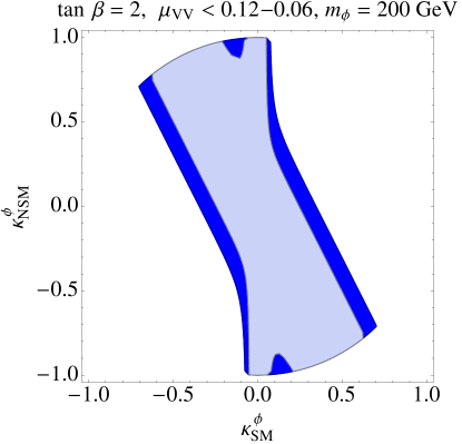
In the left panel of Fig. 1 we show the constraints on $\kappa^{h}_{\rm NSM}$ and $\kappa^{h}_{\rm S}$ for the 125 GeV Higgs boson $h$, derived from the LHC Run 1 measurements on its production cross section and branching ratios. Here we have assumed that the decay branching fractions into bottom quarks and massive vector boson cannot deviate by more than 30% from their SM values. In anticipation of our focus on the NMSSM, we concentrate on small values of $\tan\beta$. In the right panel of Fig. 1, we consider the constraints on $\kappa^{H/h_{S}}_{\rm SM}$ and $\kappa^{H/h_{S}}_{\rm NSM}$ for the non-SM-like scalars from resonance searches in the $WW$ and $ZZ$ channels Khachatryan:2015cwa , assuming production from gluon fusion processes.

First note that the singlet component of the observed 125 GeV scalar, which is only constrained by its unitarity relationship with the SM and NSM components, is allowed to be quite large. However, the NSM component is restricted to be small, except in the narrow region of parameter space where the $g_{hb\bar{b}}$ coupling is approximately equal in magnitude but with opposite sign as the SM bottom Yukawa Ferreira:2014naa . This can only occur far away from alignment and we shall not explore this region.

On the other hand, the search for exotic Higgs resonances puts strong constraints on the value of $\kappa^{H/h_{S}}_{\rm SM}$. These constraints are satisfied when $\kappa^{H/h_{S}}_{\rm SM}$ is very small, so that the decay into $WW/ZZ$ is suppressed, or when the linear combination of $\kappa^{H/h_{S}}_{\rm SM}$ and $\kappa^{H/h_{S}}_{\rm NSM}$ is such that the coupling to top quarks in Eq. (47) is small, resulting in a small production rate in the gluon fusion channel.

II.2 The $\boldsymbol{\mathbb{Z}_{3}}$ Invariant NMSSM

In this paper, we shall analyze the NMSSM under the assumption that there are no mass parameters in the superpotential, which can be ensured by imposing a $\mathbb{Z}_{3}$ symmetry under which all chiral superfields are transformed by a phase $e^{2\pi i/3}$. The superpotential then must contain only cubic combinations of superfields. The coefficients of the possible cubic terms include the usual matrix Yukawa couplings $h_{d}$, $h_{u}$ and $h_{e}$, the coupling $\lambda$ of the singlet to the doublet Higgs superfields, and the singlet Higgs superfield self-coupling parameter $\kappa$,

$$W=\lambda\widehat{S}\widehat{H}_{u}\cdot\widehat{H}_{d}+\frac{\kappa}{3}\widehat{S}^{\,3}+h_{u}\widehat{Q}\cdot\widehat{H}_{u}\,\widehat{U}_{R}^{c}+h_{d}\widehat{H}_{d}\cdot\widehat{Q}\,\widehat{D}_{R}^{c}+h_{\ell}\widehat{H}_{d}\cdot\widehat{L}\,\widehat{E}_{R}^{c}\,,$$ (49)

where we are following the notation for superfields given in Ref. Ellwanger:2009dp . In particular, we employ the dot product notation for the singlet combination of two SU(2) doublets. For example,

$$\widehat{H}_{u}\cdot\widehat{H}_{d}\equiv\epsilon_{ij}\widehat{H}_{u}^{i}\widehat{H}_{d}^{j}=\widehat{H}_{u}^{+}\widehat{H}_{d}^{-}-\widehat{H}_{u}^{0}\widehat{H}_{d}^{0}\,.$$ (50)

All Higgs mass parameters are associated with soft supersymmetry-breaking terms appearing in the scalar potential,

$$V_{\rm soft} = m_{S}^{2}S^{\dagger}S+m_{H_{u}}^{2}H_{u}^{\dagger}H_{u}+m_{H_{d}}^{2}H_{d}^{\dagger}H_{d}+\left(\lambda A_{\lambda}SH_{u}\cdot H_{d}+\tfrac{1}{3}\kappa A_{\kappa}S^{3}+{\rm h.c.}\right)$$ (51)

$$+m_{Q}^{2}Q^{\dagger}Q+m_{U}^{2}U_{R}^{c\,\dagger}U_{R}^{c}+m_{D}^{2}D_{R}^{c\,\dagger}D_{R}^{c}+M_{L}^{2}L^{\dagger}L+m_{E}^{2}E_{R}^{c\,\dagger}E_{R}^{c}$$

$$+\left(h_{u}A_{u}Q\cdot H_{u}\,U_{R}^{c}+h_{d}A_{d}H_{d}\cdot Q\,D_{R}^{c}+h_{\ell}A_{\ell}H_{d}\cdot L\,E_{R}^{c}+{\rm h.c.}\right),$$

where the scalar component of the corresponding superfield is indicated by the same symbol but without the hat. For completeness, we also include the soft supersymmetry-breaking terms that are associated with the squark fields (where generation labels are suppressed).

The Higgs scalar potential receives contributions from (i) soft supersymmetry-breaking terms in the scalar potential given in Eq. (51), (ii) from the supersymmetry-conserving $D$-terms, which depend quadratically on the weak gauge couplings, and (iii) from the supersymmetry-conserving $F$-terms associated with the scalar components of the derivatives of the superpotential with respect to the Higgs, quark and lepton superfields. Explicitly, the supersymmetry-conserving contributions to the Higgs scalar potential are given by

$$V_{\rm SUSY} = \tfrac{1}{8}(g^{2}+g^{\prime\,2})(H_{u}^{\dagger}H_{u}-H_{d}^{\dagger}H_{d})^{2}+\tfrac{1}{2}g^{2}|H_{d}^{\dagger}H_{u}|^{2}+|\lambda|^{2}|H_{u}\cdot H_{d}|^{2}$$ (52)

$$+|\lambda|^{2}S^{\dagger}S(H_{u}^{\dagger}H_{u}+H_{d}^{\dagger}H_{d})+|\kappa|^{2}(S^{\dagger}S)^{2}+(\kappa^{*}\lambda S^{*\,2}H_{u}\cdot H_{d}+{\rm h.c.})\,.$$

In the MSSM, the quartic terms of the Higgs scalar potential are proportional to gauge couplings. As a result, the tree-level mass of the observed SM-like Higgs boson can be no larger than $m_{Z}$. To obtain the observed Higgs mass of 125 GeV, significant radiative loop corrections (dominated by loops of top quarks and top squarks) must be present. A novel feature of the NMSSM is the appearance of tree-level contributions to the Higgs doublet quartic couplings that do not depend on the gauge couplings. The new quartic couplings in $V_{\rm SUSY}$ play a very important role in the Higgs phenomenology. Moreover, they provide a new tree-level source for the mass of the SM-like Higgs boson such that the observed 125 GeV mass can be achieved without the need of large radiative corrections. The structure of the scalar potential of the NMSSM allows for the alignment of one of the mass eigenstates of the CP-even Higgs bosons with the Higgs basis field $H_{1}$ (which possesses the full Standard Model VEV), while at the same time yielding a sizable tree-level contribution to the observed Higgs mass naturally, without resorting to large radiative corrections.

To simplify the analysis, we henceforth assume that the Higgs scalar potential and vacuum are CP-conserving. That is, given the Higgs potential,

$$\mathcal{V}=V_{\rm SUSY}+V^{(1)}_{\rm soft}\,,$$ (53)

where $V^{(1)}_{\rm soft}$ is the first line of Eq. (51), we assume that all the parameters of $\mathcal{V}$ can be chosen to be real. The CP conservation of the vacuum can be achieved by assuming that the product $\lambda\kappa$ is real and positive, as shown in Ellis:1988er . Minimizing the Higgs potential, the neutral Higgs fields acquire VEVs denoted by Eqs. (2) and (38). The non-zero singlet VEV, $v_{s}$, yields effective $\mu$ and $B$ parameters,

$$\mu\equiv\lambda v_{s}\,,\qquad B\equiv A_{\lambda}+\kappa v_{s}\,.$$ (54)

Conditions for the minimization of the Higgs potential allows one to express the quadratic mass parameters $m_{S}^{2}$, $m_{H_{u}}^{2}$ and $m_{H_{d}}^{2}$ in terms of the VEVs $v_{u}$, $v_{d}$, $v_{s}$, the $A$-parameters $A_{\lambda}$ and $A_{\kappa}$, and the dimensionless couplings that appear in the Higgs potential. Using Eq. (54),

$$m^{2}_{H_{d}} = \mu B\frac{v_{u}}{v_{d}}-\mu^{2}-\tfrac{1}{2}\lambda^{2}v_{u}^{2}+\tfrac{1}{8}(g^{2}+g^{\prime\,2})(v_{u}^{2}-v_{d}^{2})\,,$$ (55)

$$m^{2}_{H_{u}} = \mu B\frac{v_{d}}{v_{u}}-\mu^{2}-\tfrac{1}{2}\lambda^{2}v_{d}^{2}+\tfrac{1}{8}(g^{2}+g^{\prime\,2})(v_{d}^{2}-v_{u}^{2})\,,$$ (56)

$$m^{2}_{S} = \tfrac{1}{2}\mu B\frac{v_{d}v_{u}}{v^{2}_{s}}+\tfrac{1}{2}\lambda\kappa v_{d}v_{u}-\tfrac{1}{2}\lambda^{2}(v_{d}^{2}+v_{u}^{2})-\kappa A_{\kappa}v_{s}-2\kappa^{2}v_{s}^{2}\,.$$ (57)

The Higgs mass spectrum can now be determined from Eq. (53) by expanding the Higgs fields about their VEVs. Eliminating the Higgs squared-mass parameters using Eqs. (55)–(57), we obtain squared-mass matrices for the CP-even and the CP-odd scalars, respectively.

To analyze the alignment conditions of the NMSSM Higgs sector, we compute the squared-mass matrices of the CP-even and the CP-odd neutral Higgs bosons in the Higgs basis. It is convenient to introduce the squared-mass parameter $M_{A}^{2}$, which corresponds to the squared-mass of the CP-odd scalar in the MSSM,

$$M_{A}^{2}\equiv\frac{\mu B}{s_{\beta}c_{\beta}}\,,$$ (58)

where $s_{\beta}\equiv\sin\beta=v_{u}/v$ and $c_{\beta}\equiv\cos\beta=v_{d}/v$. In the $\{H^{\rm SM},H^{\rm NSM},H^{\rm S}\}$ basis defined in Eq. (3), the tree-level CP-even symmetric squared-mass matrix is given by

$$\mathcal{M}^{2}_{S} = \!\!\!\left(\begin{array}[]{ccc}\overline{M}_{Z}^{\lower 2.0pt\hbox{$\scriptstyle\,2$}}c^{2}_{2\beta}+\frac{1}{2}\lambda^{2}v^{2}&\quad-\overline{M}_{Z}^{\lower 2.0pt\hbox{$\scriptstyle\,2$}}s_{2\beta}c_{2\beta}&\sqrt{2}\lambda v\mu\left(1-\frac{M_{A}^{2}}{4\mu^{2}}s^{2}_{2\beta}-\frac{\kappa}{2\lambda}s_{2\beta}\right)\\[15.0pt] &\quad M_{A}^{2}+\overline{M}_{Z}^{\lower 2.0pt\hbox{$\scriptstyle\,2$}}s^{2}_{2\beta}&-\frac{1}{\sqrt{2}}\lambda v\mu c_{2\beta}\left(\frac{M_{A}^{2}}{2\mu^{2}}s_{2\beta}+\frac{\kappa}{\lambda}\right)\\[15.0pt] &&\ \ \tfrac{1}{4}\lambda^{2}v^{2}s_{2\beta}\left(\frac{M_{A}^{2}}{2\mu^{2}}s_{2\beta}-\frac{\kappa}{\lambda}\right)+\frac{\kappa\mu}{\lambda}\left(A_{\kappa}+\frac{4\kappa\mu}{\lambda}\right)\end{array}\right),$$ (62)

where we have introduced the squared-mass parameter,

$$\overline{M}_{Z}^{\lower 2.0pt\hbox{$\scriptstyle\,2$}}\equiv m_{Z}^{2}-\tfrac{1}{2}\lambda^{2}v^{2}\,,$$ (64)

and we have employed the shorthand notation, $c_{2\beta}=\cos 2\beta$ and $s_{2\beta}\equiv\sin 2\beta$. The matrix elements below the diagonal have been omitted since their values are fixed by the symmetric property of $\mathcal{M}^{2}_{S}$.

Including the leading one-loop stop contributions, the elements of the CP-even Higgs squared-mass matrix $\mathcal{M}_{S}^{2}$ involving the Higgs doublet components are 

$$\!\!\!\!\!\!\!\!\mathcal{M}^{2}_{11} = \overline{M}_{Z}^{\lower 2.0pt\hbox{$\scriptstyle\,2$}}c^{2}_{2\beta}+\tfrac{1}{2}\lambda^{2}v^{2}+\frac{3v^{2}s_{\beta}^{4}h_{t}^{4}}{8\pi^{2}}\left[\ln\left(\frac{M_{S}^{2}}{m_{t}^{2}}\right)+\frac{X_{t}^{2}}{M_{S}^{2}}\left(1-\frac{X_{t}^{2}}{12M_{S}^{2}}\right)\right]$$ (65)

$$\!\!\!\!\!\!\!\!\mathcal{M}^{2}_{22} = M_{A}^{2}+s_{2\beta}^{2}\left\{\overline{M}_{Z}^{\lower 2.0pt\hbox{$\scriptstyle\,2$}}+\frac{3v^{2}h_{t}^{4}}{32\pi^{2}}\left[\ln\left(\frac{M_{S}^{2}}{m_{t}^{2}}\right)+\frac{X_{t}Y_{t}}{M_{S}^{2}}\left(1-\frac{X_{t}Y_{t}}{12M_{S}^{2}}\right)\right]\right\}\,,$$ (66)

$$\!\!\!\!\!\!\!\!\mathcal{M}^{2}_{12} = -s_{2\beta}\left\{\overline{M}_{Z}^{\lower 2.0pt\hbox{$\scriptstyle\,2$}}c_{2\beta}-\frac{3v^{2}s_{\beta}^{2}h_{t}^{4}}{16\pi^{2}}\biggl{[}\ln\left(\frac{M_{S}^{2}}{m_{t}^{2}}\right)+\frac{X_{t}(X_{t}+Y_{t})}{2M_{S}^{2}}-\frac{X_{t}^{3}Y_{t}}{12M_{S}^{4}}\biggr{]}\right\}\,,$$ (67)

where $M_{S}$ is the geometric mean of the two stop mass-eigenstates, $X_{t}=A_{t}-\mu\cot\beta$ and $Y_{t}=A_{t}+\mu\tan\beta$.

In the CP-odd scalar sector, since we identify $A^{\rm SM}$ as the massless neutral Goldstone boson, the physical CP-odd Higgs bosons are identified by diagonalizing a $2\times 2$ symmetric matrix. In the $\{A^{\rm NSM},A^{\rm S}\}$ basis defined in Eq. (4), the tree-level CP-odd symmetric squared-mass matrix is given by

$$\mathcal{M}^{2}_{P} = \left(\begin{array}[]{cc}M_{A}^{2}&\qquad\frac{1}{\sqrt{2}}\lambda v\left(\displaystyle\frac{M_{A}^{2}}{2\mu}s_{2\beta}-\displaystyle\frac{3\kappa\mu}{\lambda}\right)\\[12.0pt] \frac{1}{\sqrt{2}}\lambda v\left(\displaystyle\frac{M_{A}^{2}}{2\mu}s_{2\beta}-\displaystyle\frac{3\kappa\mu}{\lambda}\right)&\qquad\frac{1}{2}\lambda^{2}v^{2}s_{2\beta}\left(\displaystyle\frac{M_{A}^{2}}{4\mu^{2}}s_{2\beta}+\displaystyle\frac{3\kappa}{2\lambda}\right)-\displaystyle\frac{3\kappa A_{\kappa}\mu}{\lambda}\\ \end{array}\right)\,.$$ (70)

We denote the CP-odd Higgs mass-eigenstate fields by $A$ and $A_{S}$, where $A$ is the dominantly doublet CP-odd scalar field and $A_{S}$ is the dominantly singlet CP-odd scalar field.

For completeness, we record the mass of the charged Higgs boson,

$$m^{2}_{H^{\pm}}=M_{A}^{2}+m_{W}^{2}-\tfrac{1}{2}\lambda^{2}v^{2}\,,$$ (71)

in terms of the squared-mass parameter $M_{A}^{2}$ [cf. Eq. (58)].

Exact alignment can be achieved if the following two conditions are fulfilled:

$$\mathcal{M}^{2}_{12} = \frac{1}{\tan\beta}\left[\mathcal{M}^{2}_{11}-c_{2\beta}m_{Z}^{2}-\lambda^{2}v^{2}s_{\beta}^{2}\right]+\frac{3v^{2}s_{\beta}^{2}h_{t}^{4}\mu X_{t}}{16\pi^{2}M_{S}^{2}}\left(1-\frac{X_{t}^{2}}{6M_{S}^{2}}\right)=0\ ,$$ (72)

$$\mathcal{M}^{2}_{13} = \sqrt{2}\lambda v\mu\left(1-\frac{M_{A}^{2}s_{2\beta}^{2}}{4\mu^{2}}-\frac{\kappa s_{2\beta}}{2\lambda}\right)=0\;,\,$$ (73)

after noting that $Y_{t}-X_{t}=\mu/(s_{\beta}c_{\beta})$. In what follows, we will study under what conditions alignment can occur in regions of parameter space where no large cancellation is necessary to achieve the spontaneous breaking of electroweak symmetry.

(a)

(b)

Figure 2: Left panel : The blue shaded band displays the values of $\lambda$ as a function of $\tan\beta$, necessary for alignment for $m_{h}=125\pm 3$ GeV. Also shown in the figure as a green band are values of $\lambda$ that lead to a tree-level Higgs mass of $125\pm 3$ GeV. Right panel : Values of $M_{S}$ necessary to obtain a 125 GeV mass for values of $\lambda$ fixed by the alignment condition and stop mixing parameter $X_{t}=0$ and $X_{t}=M_{S}$. The dominant two-loop corrections are included.

Since $|\mu|^{2}$ is the diagonal Higgs squared-mass parameter at tree-level in the absence of supersymmetry breaking, it is necessary to demand that $|\mu|\ll M_{S}$. Furthermore, the SM-like Higgs mass in the limit of small mixing is approximately given by $\mathcal{M}^{2}_{11}$ [cf. Eq. (65)]. The one-loop radiative stop corrections to $\mathcal{M}^{2}_{12}$ exhibited in Eq. (67) that are not absorbed in the definition of $\mathcal{M}^{2}_{11}$ are suppressed by $\mu/M_{S}$ (in addition to the usual loop suppression factor), as shown in Eq. (72), and thus can be neglected (assuming $\tan\beta$ is not too large) in obtaining the condition of alignment. Hence, satisfying Eq. (72) fixes $\lambda$, denoted by $\lambda^{\rm alt}$, as a function of $m_{h}$, $m_{Z}$ and $\tan\beta$,

$$(\lambda^{\rm alt})^{2}=\frac{m_{h}^{2}-m_{Z}^{2}c_{2\beta}}{v^{2}s_{\beta}^{2}}\ .$$ (74)

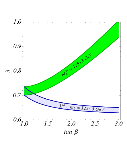
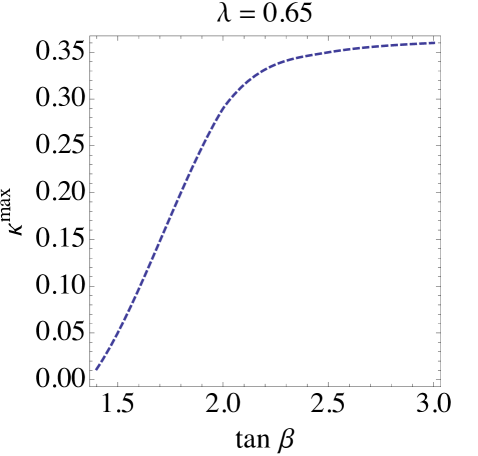
The above condition may only be fulfilled in a very narrow band of values of $\lambda=0.6$ – $0.7$ over the $\tan\beta$ range of interest. This is clearly shown in Fig. 2, where the blue band exhibits the values of $\lambda$ that lead to alignment as a function of $\tan\beta$. It is noteworthy that such values of $\lambda$ are compatible with the perturbative consistency of the theory up to the Planck scale, and lead to large tree-level corrections to the Higgs mass for values of $\tan\beta$ of order one. This is shown by the green band, which depicts the values of $\lambda$ necessary to obtain a tree-level Higgs mass $m_{h}=125\pm 3$ GeV as a function of $\tan\beta$.

The separation of the green and blue bands in Fig. 2 for a given value of $\tan\beta$ is an indication of the required radiative corrections necessary to achieve a Higgs mass consistent with observations. In particular, for a given Higgs mass, the value of the stop loop corrections $\Delta_{\tilde{t}}$ necessary to lift $\mathcal{M}^{2}_{11}$ to $m_{h}^{2}$, obtained from Eqs. (65) and (74), is given by

$$\Delta_{\tilde{t}}=-c_{2\beta}\left(m_{h}^{2}-m_{Z}^{2}\right)\ .$$ (75)

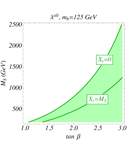
In the right panel of Fig. 2 we show the necessary values of $M_{S}$ as a function of $\tan\beta$ to obtain the required radiative corrections for $m_{h}=125$ GeV, for two different values of the stop mass mixing parameter, $X_{t}=0$ and $X_{t}=M_{S}$. We see that for moderate values of $X_{t}$ the values of $M_{S}$ relevant for the radiative corrections to the Higgs mass parameter remain below 1 TeV for values of $\tan\beta$ below about 3. In the following we shall concentrate on this interesting region, which is complementary to the one preferred in the MSSM.

It should be noted that there are previous studies on the relation between fine-tunings and a SM-like Higgs boson in the NMSSM Farina:2013fsa ; Gherghetta:2014xea . These works focus on the regime where $\lambda$ is large and $m_{h}^{tree}=125$ GeV, i.e. the green band region in Fig. 2(a), and conclude that a SM-like 125 GeV Higgs requires decoupling of supersymmetric particles, which in turn leads to more fine-tuning in the Higgs mass. In contrast, in the present work we allow for moderate contributions from the stop loops to raise the Higgs mass to keep $\lambda\sim 0.7$, which yields a SM-like Higgs boson via alignment without decoupling. The stop mass parameters do not need to be large, as can be seen in Fig. 2(b), giving rise to natural electroweak symmetry breaking.

(a)

(b)

Figure 3: Left panel : Values of $M_{A}$ leading to a cancellation of the mixing of the singlet with the SM-like Higgs boson in the Higgs basis, shown in the $|\mu|$–$\tan\beta$ plane. The values of $\lambda$ were fixed so that the alignment condition among the doublet components is fulfilled. Values of $\kappa=\tfrac{1}{2}\lambda$ close to the edge of the perturbativity consistency region were selected. Right Panel: Maximum values of $\kappa$ consistent with perturbativity as a function of $\tan\beta$ for $\lambda=0.65$.

The previous discussion assumed implicitly that the singlets are either decoupled or not significantly mixed with the CP-even doublet scalars, which is why we only concentrated on the behavior of the mass matrix element $\mathcal{M}^{2}_{12}$. If we now consider the case of a light singlet state, then the second condition of alignment, namely small mixing between the singlet and the SM-like CP-even Higgs boson, requires $\mathcal{M}^{2}_{13}\simeq 0$, as indicated in Eq. (73). This yields the following condition:

$$\frac{M_{A}^{2}s_{2\beta}^{2}}{4\mu^{2}}+\frac{\kappa s_{2\beta}}{2\lambda}=1\ .$$ (76)

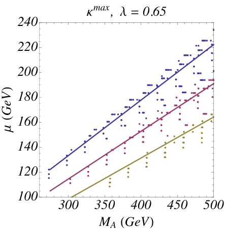
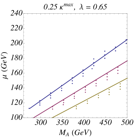
We shall take $\lambda\simeq 0.65$, as required by the alignment condition given in Eq. (74), and $\kappa\leq\tfrac{1}{2}\lambda$, where the latter is a consequence of the perturbative consistency of the theory up to the Planck scale, as shown in the right panel of Fig. 3. It follows that in order to satisfy Eq. (76) the mass parameter $M_{A}$ must be approximately correlated with the parameter $\mu$,

$$M_{A}\sim\frac{2|\mu|}{s_{2\beta}}\ .$$ (77)

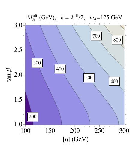
In the parameter regime where $100\mathrel{\raise 1.29167pt\hbox{$<$\kern-7.5pt\lower 4.30554pt\hbox{$\sim$}}}|\mu|\mathrel{\raise 1.29167pt\hbox{$<$\kern-7.5pt\lower 4.30554pt\hbox{$\sim$}}}300$ GeV (so that no tree-level fine tuning is necessary to achieve electroweak symmetry breaking) and $1\mathrel{\raise 1.29167pt\hbox{$<$\kern-7.5pt\lower 4.30554pt\hbox{$\sim$}}}\tan\beta\mathrel{\raise 1.29167pt\hbox{$<$\kern-7.5pt\lower 4.30554pt\hbox{$\sim$}}}3$, we see that $M_{A}$ is somewhat larger than $|\mu|$. This is shown in the left panel of Fig. 3, in which the values of $M_{A}$ leading to the cancellation of the mixing with the singlet CP-even Higgs state is shown in the $|\mu|$–$\tan\beta$ plane. Here, we have chosen a value of $\kappa\simeq\tfrac{1}{2}\lambda$, which as mentioned above is about the maximal value of $\kappa$ that could be obtained for $\tan\beta\stackrel{{\scriptstyle>}}{{{}_{\sim}}}2$ if the theory is to remain perturbative up to the Planck scale.

The condition $\mathcal{M}^{2}_{13}=0$ has implications for the value of $\mathcal{M}^{2}_{23}$, which governs the mixing between the singlet CP-even state and the non-standard CP-even component of the doublet states. More precisely, if $\mathcal{M}^{2}_{13}$ vanishes, as implied by the condition of alignment given in Eq. (73), then

$$\mathcal{M}^{2}_{23}=-\sqrt{2}\lambda v\mu\frac{c_{2\beta}}{s_{2\beta}}\ ,$$ (78)

leading to a non-vanishing mixing effect between the light singlet and the heaviest CP-even Higgs boson when $\tan\beta\neq 1$. For the range of values of the parameters employed in Fig. 3, the ratio $\mathcal{M}^{2}_{23}/M_{A}^{2}\ll 1$.

In practice, for $\lambda\simeq 0.65$, the inequality $\mathcal{M}^{2}_{12}\ll\mathcal{M}^{2}_{13}$ holds unless the mass parameters $M_{A}$ and $\mu$ are tuned to obtain almost exact alignment. Hence, based on the discussion above, we shall henceforth assume that the following hierarchy among the elements of the CP-even Higgs squared-mass matrix is fulfilled close to the alignment limit,

$$\mathcal{M}^{2}_{12}\ \ll\ \ \mathcal{M}^{2}_{13}\ \ \ll\ \ \mathcal{M}^{2}_{23},\mathcal{M}^{2}_{11},\mathcal{M}^{2}_{33}\ \ \ll\ \ \mathcal{M}^{2}_{22}.$$ (79)

Given the above observations, it is not difficult to see that all mixing angles in the CP-even Higgs mixing matrix are small. Therefore, the mass eigenstate $h$, whose predominant component is $H^{\rm SM}$, is SM-like, whereas the predominant components of the other two eigenstates $H$ and $h_{S}$ are $H^{\rm NSM}$ and $H^{\rm S}$, respectively. In particular,

$$m_{h}^{2}\simeq\mathcal{M}^{2}_{11}\;,\;\;\;\;\;\;\;\;m_{H}^{2}\simeq\mathcal{M}^{2}_{22}\;,\;\;\;\;\;\;\;\;m_{h_{S}}^{2}\simeq\mathcal{M}^{2}_{33}\;,$$ (80)

and the hierarchy of masses

$$m_{H}^{2}\ \gg\ m_{h}^{2},\ m_{h_{S}}^{2}$$ (81)

is fulfilled in the region of parameter space under consideration. Using Eqs. (28)–(30) and ignoring terms of order $\epsilon_{1}\equiv\mathcal{M}^{2}_{12}/\mathcal{M}^{2}_{22}$ and $\epsilon_{2}\equiv\mathcal{M}_{13}^{2}\mathcal{M}_{23}^{2}/\mathcal{M}_{22}^{4}$, we derive the following approximate relationship between the interaction and mass eigenstates,

$$\left(\begin{array}[]{c}h\\ H\\ h_{S}\end{array}\right)\simeq\left(\begin{array}[]{ccc}1&\ -\eta\eta^{\prime}&\,\,\,\,\phantom{-}\eta^{\prime}\\ {\cal{O}}(\epsilon)&-1&\,\,\,\,-\eta\\ -\eta^{\prime}&\ -\eta&\,\,\,\,\phantom{-}1\end{array}\right)\left(\begin{array}[]{c}H^{\rm SM}\\ H^{\rm NSM}\\ H^{\rm S}\end{array}\right)\ ,$$ (82)

where the elements of the CP-even Higgs mixing matrix are expressed in terms of

$$-\kappa^{H}_{S}=\eta = \frac{\mathcal{M}^{2}_{23}}{m_{H}^{2}},$$ (83)

$$\kappa^{h}_{S}=\eta^{\prime} = \frac{\mathcal{M}^{2}_{13}}{m_{h}^{2}-\mathcal{M}^{2}_{33}}\,,$$ (84)

and $\mathcal{O}(\epsilon)$ denotes a linear combination of terms of order $\epsilon_{1}$ and $\epsilon_{2}$, respectively. In Eq. (82), we have kept all terms in the mixing matrix up to quadratic in the small quantities $\eta$ and $\eta^{\prime}$. Given the assumed hierarchy of Eq. (79), the $\mathcal{O}(\epsilon)$ terms are at best of the same order as quantities that are cubic in $\eta$ and $\eta^{\prime}$ and hence are truly negligible. This then tells us that the following approximate relationship exists between the mixing angles defined in Eq. (19),

$$s_{12}\simeq-s_{13}s_{23}\,,$$ (85)

and the alignment limit in the hierarchy of Eq. (79) is primarily governed by two small mixing angles.

Eq. (82) provides a useful guide for understanding the Higgs phenomenology in our numerical study. In particular, there are correlations among the different matrix elements. For example,

$$\kappa^{h}_{\rm S} \simeq -\kappa^{h_{S}}_{\rm SM}\ ,$$ (86)

$$\kappa^{h}_{\rm NSM} \simeq \kappa^{h}_{\rm S}\kappa^{H}_{\rm S}\ ,$$ (87)

$$\kappa^{H}_{\rm S} \simeq \kappa^{h_{S}}_{\rm NSM}\ .$$ (88)

In light of Eqs. (77) and (78), it follows that [cf. Eqs. (83) and (84)]:

$$\kappa^{H}_{\rm S}\simeq\kappa^{h_{S}}_{\rm NSM}\simeq\frac{\lambda v}{2\sqrt{2}\,\mu}c_{2\beta}s_{2\beta}\;.$$ (89)

We have previously argued that values of $\lambda\simeq 0.6-0.7$ are preferred from both the perspective of Higgs phenomenology as well as perturbative consistency of the NMSSM up to the Planck scale. In addition we note that the range of $\mu$ is rather restricted: $|\mu|>100$ GeV, in order to fulfill the LEP chargino bounds, however $\mu$ cannot be too large in order to preserve a natural explanation for electroweak symmetry breaking. Hence, we can see from Eq. (89) that if for example $|\mu|\stackrel{{\scriptstyle<}}{{{}_{\sim}}}200$ GeV, then

$$0.15\stackrel{{\scriptstyle<}}{{{}_{\sim}}}|\kappa_{\rm NSM}^{h_{S}}|\stackrel{{\scriptstyle<}}{{{}_{\sim}}}0.3\ ,$$ (90)

which implies that all mixing angles are small if the conditions of alignment are imposed. For the small values of $\kappa$ consistent with a perturbative extension of the theory up to the Planck scale (see Fig. 3), the above estimate continues to hold even after the $\kappa$-induced effects as well as the corrections associated with the $h_{S}$ mass are included.

II.3 Spectrum of the Higgs Sector Near the Alignment Limit

Close to the alignment limit, the mass parameter $M_{A}\simeq 2|\mu|/s_{2\beta}$. Since $|\mu|$ must be larger than about 100 GeV in order to fulfill the current LEP constraints on the chargino masses, it follows that for $\tan\beta\geq 2$, the CP-odd Higgs mass must be larger than about 250 GeV. We conclude that $M_{A}^{2}\gg m_{h}^{2}$. In light off this observation, the spectrum of neutral Higgs bosons near the alignment limit may be approximated by 

• A SM-like CP-even Higgs boson state of mass $m_{h}^{2}=(125~{}{\rm GeV})^{2}\simeq\mathcal{M}^{2}_{11}\ll M_{A}^{2}$.

• A heavy CP-even Higgs boson state $H$ of mass $m_{H}\simeq M_{A}$.

• A heavy CP-odd Higgs boson state $A$ of mass $m_{A}\simeq M_{A}$.

• Light, mostly singlet-like CP-even and CP-odd Higgs boson states with masses

  $$m_{h_{S}}^{2} \simeq \frac{\kappa\mu}{\lambda}\left(A_{\kappa}+\frac{4\kappa\mu}{\lambda}\right)+\frac{\lambda^{2}v^{2}M_{A}^{2}}{8\mu^{2}}s_{2\beta}^{4}-\tfrac{1}{4}{v^{2}}\kappa\lambda(3-2s_{2\beta}^{2})s_{2\beta}-\tfrac{1}{2}v^{2}\kappa^{2}\frac{\mu^{2}}{M_{A}^{2}}c_{2\beta}^{2}\,,$$

  $$m_{A_{S}}^{2} \simeq 3\kappa\left[\tfrac{3}{4}\lambda v^{2}s_{2\beta}-\mu\left(\frac{A_{\kappa}}{\lambda}+\frac{3v^{2}\kappa\mu}{2M_{A}^{2}}\right)\right]\,.$$ (92)

It is interesting to note that the singlet-like Higgs masses depend on the parameter $A_{\kappa}$ which is not restricted by the conditions of alignment. As such, these masses are not correlated with the other Higgs boson masses. For positive values of $\mu$ and $\kappa$, larger values of $A_{\kappa}$ lead to an increase in $m_{h_{S}}^{2}$ and a decrease in $m_{A_{S}}^{2}$. Therefore, for fixed values of the other parameters, the value of $A_{\kappa}$ is restricted by the requirement of non-negative $m_{h_{S}}^{2}$ and $m_{A_{S}}^{2}$. In particular, due to the anti-correlation in the behavior of $m_{h_{S}}^{2}$ and $m_{A_{S}}^{2}$ with $A_{\kappa}$, the maximal possible value, $(m_{h_{S}}^{2})_{\rm max}$, is achieved when $m_{A_{S}}^{2}=0$. Likewise, the maximal value, $(m_{A_{S}}^{2})_{\rm max}$, is achieved when $m_{h_{S}}^{2}=0$. Using Eqs. (• ‣ II.3) and (92) to eliminate $A_{\kappa}$, and making use of Eq. (76) in the alignment limit to eliminate $\mu^{2}$,

$$m^{2}_{A_{S}}+3m^{2}_{h_{S}}\simeq\frac{3M_{A}^{2}s_{2\beta}^{2}}{1-\tfrac{1}{2}\kappa s_{2\beta}/\lambda}\left[\frac{\kappa^{2}}{\lambda^{2}}+\frac{\lambda^{2}v^{2}}{2M_{A}^{2}}\left(1-\frac{\kappa^{2}}{\lambda^{2}}\right)\right]\,.$$ (93)

(a)

(b)

Figure 4: Values of the singlet CP-even Higgs mass $m_{h_{S}}$ for $\tan\beta=2$ (left panel) and $\tan\beta=3$ (right panel) in the plane of $m_{A}$ vs. $m_{A_{S}}$, imposing a SM-like Higgs boson with a mass of 125 GeV (with $\lambda$ and $\mu$ satisfying the alignment conditions and $\kappa=\tfrac{1}{2}\lambda$).

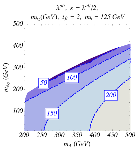
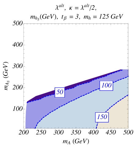
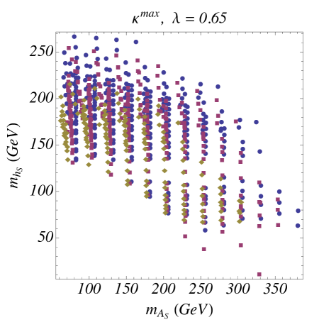
In the parameter region of interest, $\kappa\leq\tfrac{1}{2}\lambda$ and $s_{2\beta}$ is near 1. Close to the alignment limit (where $\lambda\simeq 0.65$), we have noted above that $m_{A}^{2}\simeq M_{A}^{2}\gg\tfrac{1}{2}\lambda^{2}v^{2}$, in which case $(m_{h_{S}}^{2})_{\rm max}\stackrel{{\scriptstyle<}}{{{}_{\sim}}}\tfrac{1}{3}m_{A}^{2}$ and $(m_{A_{S}}^{2})_{\rm max}\mathrel{\raise 1.29167pt\hbox{$<$\kern-7.5pt\lower 4.30554pt\hbox{$\sim$}}}m_{A}^{2}$. In the left and right panels of Fig. 4, we display the contours of the singlet-like CP-even Higgs mass in the $m_{A}$–$m_{A_{S}}$ plane for $\kappa\simeq\tfrac{1}{2}\lambda^{\rm alt}$ and for $\tan\beta=2$ and $\tan\beta=3$, respectively. Whereas $m_{A_{S}}$ may become of order $m_{A}$ for low values of $\tan\beta$ (i.e. for $s_{2\beta}\simeq 1$), the singlet CP-even Higgs mass remains below $\tfrac{1}{2}m_{A}$ over most of the parameter space, in agreement with Eq. (93).

III Numerical Results of Masses and Mixing Angles

In the previous section, we have performed an analytical study of the implications of the alignment limit on the masses and mixing angles of the Higgs mass eigenstates. To obtain a more accurate picture, we complement the above analysis with the results obtained from a numerical study, including all relevant corrections to the CP-even and CP-odd Higgs squared-mass matrix elements. In our numerical evaluation we have used the code NMHDecay Ellwanger:2005dv and the code Higgsbounds Bechtle:2013wla included in NMSSMTools NMSSMTools . We keep parameter points that are consistent with the present constraints coming from measurements on properties of the 125 GeV Higgs boson $h$, as well as those coming from searches for the new Higgs bosons $H$ and $h_{S}$, which impose constraints on $\kappa^{\phi}_{i}$ similar to those shown in Fig. 1. We do not impose flavor constraints since they depend on the flavor structure of the supersymmetry breaking parameters, which has only a very small impact on Higgs physics. Moreover, in most of our analysis we have assumed the gaugino mass parameters to be large by fixing the electroweak gaugino masses to 500 GeV and the gluino mass to 1.5 TeV. Since the Higgsino mass parameter is small in our region of interest, the resulting dark matter relic density due to the lightest supersymmetric particle (LSP) tends to be smaller than the observed value, which implies that other particles outside of the NMSSM (e.g. axions) must contribute significantly to the dark matter relic density. Alternatively, it is possible to saturate the observed relic density with the LSP by lowering the value of the electroweak gaugino masses chosen above. We have also fixed $\mu>0$, but we have checked that the generic behavior discussed in this work does not depend on the sign of $\mu$, as can be understood analytically from the expressions given in Section II. The implications of lowering the gaugino masses to obtain the proper relic density will be briefly discussed below.

(a)

(b)

Figure 5: Values of the mass parameters $M_{A}$ and $\mu$ consistent with the current LHC constraints on the SM-like Higgs properties, for values of $\kappa=\kappa^{\rm max}$, the maximal value of $\kappa$ leading to perturbative consistency of the theory up to the Planck scale (left panel) and for $\kappa=\tfrac{1}{4}\kappa^{\rm max}$. Solid lines represent the alignment condition, Eq. (76), and the colors blue, red and yellow represent values of $\tan\beta=2$, 2.5 and 3, respectively.

In our numerical study, we have chosen $\lambda=0.65$. The stop spectrum has been determined to reproduce the observed Higgs mass, assuming small stop mixing, and we have varied all other relevant parameters allowed by the above constraints. As shown in Fig. 2, for $\tan\beta\geq 2$ and common values of the left- and right-stop supersymmetry breaking parameters, the assumption of small stop mixing leads to stops that are heavier than about 600 GeV and essentially decouple from Higgs phenomenology. For $\tan\beta\simeq 2$, larger values of the stop mixing may lead to lighter stops, resulting in a variation of the Higgs production cross section in the gluon fusion channel. We shall briefly comment on such possible effects below.

As discussed in Section II.2, a value of $\lambda\simeq 0.65$ leads to an approximate cancellation of the mixing between the SM and non-SM doublet components for all moderate or small values of $\tan\beta$ and allows a perturbative extension of the theory up to energy scales of order the Planck scale. Moreover, close to the alignment limit, the SM-like Higgs mass receives a significant tree-level contribution, which reduces the need for large radiative corrections associated with heavy stops, as shown in Fig. 2. Due to the strong perturbativity constraints shown in Fig. 2, we focus on the NMSSM parameter regime with $\tan\beta=2,2.5$ and 3, which we henceforth display in blue, red and yellow colors, respectively.

The allowed values of $M_{A}$ and $\mu$ are shown in Fig. 5, for the values of $\kappa=\kappa^{\rm max}$, the maximal values consistent with the perturbative consistency of the theory up to the Planck scale (left panel) and for values of $\kappa=\tfrac{1}{4}\kappa^{\rm max}$ (right panel). The solid lines represent the correlation between $M_{A}$ and $\mu$ necessary to get alignment at tree-level [cf. Eq. (76)]. The dots represent the allowed values of these parameters as obtained from NMSSMTools. We find that the present constraints on the SM-like Higgs properties allow values of $M_{A}$ and $\mu$ that deviate not more than 10% from the alignment condition specified in Eq. (76).

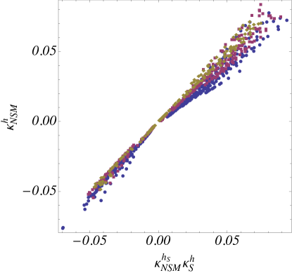
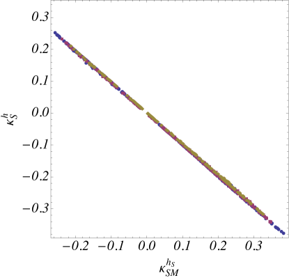
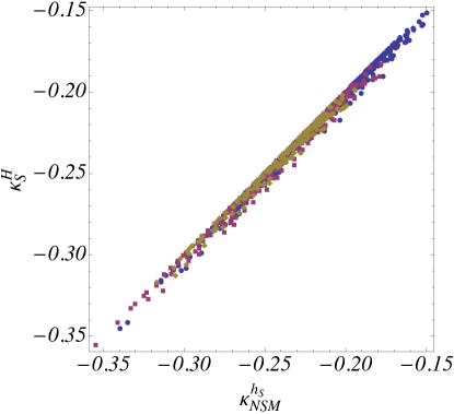
The correlations obtained in Eqs. (86)–(88) among the interaction eigenstate components, $H^{\rm SM}$, $H^{\rm NSM}$ and $H^{\rm S}$, of the mass-eigenstate neutral Higgs bosons are clearly displayed in Figs. 6, 7 and 8. The right panel of Fig. 6 displays the correlation between the singlet component of $h$ with the SM component of the mostly singlet state $h_{S}$, whereas the left panel exhibits the correlation between $\kappa^{h}_{\rm NSM}$ with $\kappa^{h}_{S}\kappa^{h_{S}}_{\rm NSM}$. We see the correlation given in Eq. (86) is preserved over most of the parameter space, however there are small departures from the correlations exhibited in Eqs. (86) and (87) due to neglected terms that are higher order in $\eta$ and $\eta^{\prime}$.

(a)

(b)

Figure 6: For the points allowed by LHC constraints in the left panel we plot the correlation between the non-SM doublet component of the 125 GeV Higgs state with the product of the non-SM doublet component of the mainly singlet state and the singlet component of the 125 GeV Higgs state. In the right panel we plot the correlation between the SM doublet component of the singlet state with the singlet component of the 125 GeV Higgs state. Blue, red and yellow represent values of $\tan\beta=2$, 2.5 and 3, respectively.

(a)

(b)

Figure 7: For the points allowed by LHC constraints, we show the correlation between the non-SM doublet component and the SM doublet component of the mainly singlet Higgs state. Blue, red and yellow represent values of $\tan\beta=2$, 2.5 and 3, respectively.

(a)

(b)

Figure 8: For the points allowed by LHC constraints, in the left panel we plot the correlation between the non-SM doublet component and the singlet component of the 125 GeV Higgs state. In the right panel we plot the square of the couplings of the 125 GeV Higgs state, normalized to its SM value. Blue, red and yellow represent values of $\tan\beta=2$, 2.5 and 3, respectively.

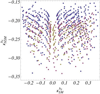
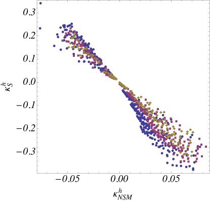
Similarly, the right panel of Fig. 7 shows the correlation between $\kappa^{h}_{\rm S}$ and $\kappa^{h_{S}}_{\rm NSM}$, with values of $0.15\stackrel{{\scriptstyle<}}{{{}_{\sim}}}|\kappa^{h}_{S}|\stackrel{{\scriptstyle<}}{{{}_{\sim}}}0.35$, as anticipated in Eq. (90). In the left panel we show the values of $\kappa^{h_{S}}_{\rm NSM}$ and $\kappa^{h_{S}}_{\rm NSM}$, which are proportional to $\eta$ and $\eta^{\prime}$ respectively. Whereas $\kappa^{h_{S}}_{\rm SM}$ can become very small in the region of alignment, there is no strong correlation between these two singlet components. There is only a weak correlation associated with the dependence of the singlet production cross section on the doublet components, which leads to negative values of $\kappa^{h_{S}}_{\rm SM}$ being somewhat more restricted than positive ones for $\mu>0$, as could be anticipated from the behavior exhibited in Fig. 1.

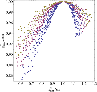
Due to the specific values of $\kappa^{h_{S}}_{\rm NSM}$ under consideration, and the correlation between $\kappa^{h}_{\rm NSM}$ and the product of $\kappa^{h}_{\rm S}\kappa^{h_{S}}_{\rm NSM}$, a mild correlation appears between the non-SM components of the SM-like Higgs, which is displayed in the left panel of Fig. 8. The largest singlet components are associated with the smallest SM component and hence the smallest values of the couplings to vector bosons. The bottom-quark coupling can be visibly suppressed in this region, but the branching ratios and signal strengths remain in the allowed region due to the suppression of the vector bosons coupling and a small enhancement of the up-quark couplings, as follows from Eqs. (46)–(48). In contrast, as shown in the right panel of Fig. 8, enhancements of the bottom couplings are more restricted due to a suppression of the $h$ branching ratios to photons and vector bosons and an additional suppression of the gluon fusion production cross section associated with smaller top-quark couplings.

IV Higgs Boson Production and Decay

The study of the properties of the 125 GeV Higgs boson and their proximity to SM expectations has been the subject of intensive theoretical and experimental analyses, and will remain one of the most important research topics at the LHC. Close to the alignment limit, and in the absence of beyond-the-SM light charged or colored particles, the properties of one of the neutral scalars (identified with the observed Higgs boson of mass 125 GeV) are nearly identical to those of the SM Higgs boson. However, as demonstrated in the right panel of Fig. 8, the current Higgs data allow for variations, of up to about 30%, of the 125 GeV Higgs boson production and decay rates with respect to the SM predictions. Such deviations can be understood as a function of the mixing of the observed SM-like Higgs boson with additional non-SM-like Higgs scalars that could be searched for at the LHC.

In this section, we shall mainly concentrate on the non-SM-like Higgs boson production and decay rates and their possible search channels at the LHC. It is noteworthy that, due to the smallness of $\kappa^{H}_{\rm SM}$, the couplings of the heavy Higgs bosons to the up and down-quarks are close to the MSSM decoupling values. In particular, using Eq. (82), the ratio of their couplings to the SM ones given by Eqs. (46)–(48) are

$$g_{HVV} \simeq \mathcal{O}(\epsilon)\,,$$

$$g_{Htt} \simeq -\frac{1}{\tan\beta}+\mathcal{O}(\epsilon)\,,$$

$$g_{Hbb} \simeq \tan\beta+\mathcal{O}(\epsilon)\,,$$ (94)

where the terms of $\mathcal{O}(\epsilon)\ll 1$ represent a linear combination of terms of order $\mathcal{M}^{2}_{12}/\mathcal{M}^{2}_{22}$ and $\mathcal{M}_{13}^{2}\mathcal{M}_{23}^{2}/\mathcal{M}_{22}^{4}$ [cf. the discussion below Eq. (81)].

Similarly, the CP-odd couplings are given approximately by their MSSM expressions,

$$g_{Att} \simeq \frac{1}{\tan\beta}\,,$$

$$g_{Abb} \simeq \tan\beta\,.$$ (95)

Finally, the $h_{S}$ couplings are given by

$$g_{h_{S}VV} = -\eta^{\prime}\,,$$

$$g_{h_{S}tt} = -\eta^{\prime}-\frac{\eta}{\tan\beta}\,,$$

$$g_{h_{S}bb} = -\eta^{\prime}+\eta\tan\beta\,.$$ (96)

Considering the typical values of the mixing angles $\eta$ and $\eta^{\prime}$, we see that the production cross section of $h_{S}$ via top-quark induced gluon fusion is generally at least an order of magnitude lower than the one for a SM-Higgs boson of the same mass. Due to the smallness of the bottom Yukawa couplings and the small values of $\tan\beta$ considered in this work, the decay branching ratios are mainly determined by the $h_{S}$ mass and will be of order of the SM ones. Therefore the present constraint on the signal strength of the production of $h_{S}$ decaying to vector bosons, $\mu_{VV}\stackrel{{\scriptstyle<}}{{{}_{\sim}}}0.1$ discussed in Section II.1 is not expected to strongly constrain this model.

(a)

(b)

Figure 9: Correlation between $m_{H}\simeq m_{A}$ and the lightest non-SM-like CP-even Higgs boson mass (left panel) and anti-correlation between the masses of the lightest non-SM-like CP-even Higgs boson and the lightest, mostly singlet CP-odd Higgs boson (right panel), for values of $\kappa=\kappa^{\rm max}$. Blue, red and yellow represent values of $\tan\beta=2$, 2.5 and 3, respectively.

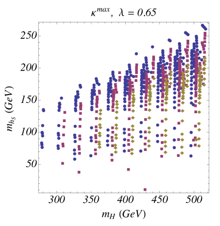
In Section II.3 we discussed the analytical constraints on the Higgs spectrum that play a crucial role in the phenomenology of the non-SM-like Higgs bosons. In Fig. 4 we showed contours of the singlet CP-even Higgs mass for different values of $M_{A}\simeq m_{A}\simeq m_{H}$ and the lightest CP-odd Higgs mass, which tends to be mostly singlet in this region of parameter space. In Fig. 9, we exhibit the correlation between the mass $m_{A}\simeq m_{H}$ of the heaviest CP-odd/even Higgs bosons (which possess a significant doublet component) and the lighter mostly singlet CP-even Higgs boson mass (left panel), and the anti-correlation between the mass of the lightest CP-odd Higgs boson (which possesses a significant singlet component) and the mostly singlet like CP-even Higgs boson (right panel). These numerical result verify the expectations based on the analytical analysis of Section II.3. In particular, these singlet-like Higgs boson masses are always smaller than $m_{A}$ and the relation

$$m_{A}\geq 2\ m_{h_{S}}$$ (97)

is fulfilled. On the other hand, the anti-correlation between the CP-odd/even mainly singlet Higgs boson masses implies that values of $m_{A_{S}}\stackrel{{\scriptstyle<}}{{{}_{\sim}}}150$ GeV constrain $m_{h_{S}}$ to be larger than about 120 GeV, while values of $m_{h_{S}}\stackrel{{\scriptstyle<}}{{{}_{\sim}}}120$ GeV imply $m_{A_{S}}\stackrel{{\scriptstyle>}}{{{}_{\sim}}}150$ GeV.

In general, large values of $M_{A}\simeq m_{A}\simeq m_{H}$ are allowed, as in the usual decoupling regime, but in this work we are mostly interested in having a SM-like Higgs boson for values of $M_{A}\mathrel{\raise 1.29167pt\hbox{$<$\kern-7.5pt\lower 4.30554pt\hbox{$\sim$}}}500$ GeV, where the non-SM-like Higgs bosons are not heavy. Given that we are interested in values of $\tan\beta\sim 2$ and $M_{A}\simeq|\mu|/s_{\beta}c_{\beta}$, this leads also to low values of $\mu$, improving the naturalness of the theory. Considering the LEP lower bound on $|\mu|$, the above relation also implies $M_{A}\stackrel{{\scriptstyle>}}{{{}_{\sim}}}250$ GeV. Therefore, the decays

$$H\to h\ h_{S},\;\;\;\;\;\;H\to h_{S}h_{S}\;\;\;\;\;\;{\rm and}\;\;\;\;\;H\to hh$$ (98)

are always allowed. However, since the coupling $g_{Hhh}$ approaches zero in the alignment limit [cf. Appendix C], the first two decay rates are in general more significant than the decay into pairs of SM-like Higgs bosons. Moreover, from Table 3 of Appendix C, it follows that when $M_{A}\simeq 2|\mu|/s_{2\beta}$ and $\kappa$ is small,

$$g_{Hhh_{S}}\simeq\sqrt{2}\ \lambda\mu\,\cot{2\beta}\;\;\;\;\;\;g_{Hh_{S}h_{S}}\simeq 4\sqrt{2}\ \eta\lambda\mu.$$ (99)

Hence, for $0.15\stackrel{{\scriptstyle<}}{{{}_{\sim}}}\eta\stackrel{{\scriptstyle<}}{{{}_{\sim}}}0.35$, these couplings are of the same order as $|\mu|$ for $2\stackrel{{\scriptstyle<}}{{{}_{\sim}}}\tan\beta\stackrel{{\scriptstyle<}}{{{}_{\sim}}}3$, which implies that these decay channels may contribute significantly to the $H$ decay width.

On the other hand, mixing between the doublet and singlet states in the CP-odd sector is also dictated by $\eta$ and hence non-vanishing. Therefore, the decay channels

$$H\to A_{S}Z\;\;\;\;\;{\rm and}\;\;\;\;\;\;A\to h_{S}Z$$ (100)

may become significant. In particular, for values of the heavy Higgs states below the $t\bar{t}$ threshold, the decay branching ratio in these channels may become dominant at low values of $\tan\beta$, for which the couplings to down-quark fermions and charged leptons are small, of the order of the corresponding SM Yukawa couplings.

(a)

(b)

Figure 10: Branching ratio of the decay of the heaviest CP-even Higgs boson into pairs of identical CP-even Higgs bosons. Blue, red and yellow represent values of $\tan\beta=2$, 2.5 and 3, respectively.

(a)

(b)

Figure 11: Branching ratios of the decay of the heavy CP-even Higgs boson into a pair of non-identical lighter CP-even Higgs bosons, $H\to hh_{S}$ (left panel) and into the lightest CP-odd Higgs boson and a $Z$ boson (right panel). Blue, red and yellow represent values of $\tan\beta=2$, 2.5 and 3, respectively.

(a)

(b)

Figure 12: Branching ratio of the decay of the heaviest CP-odd Higgs boson into a pair of non-identical Higgs bosons consisting of the lightest CP-odd Higgs boson and one of the two lighter CP-even Higgs bosons. Blue, red and yellow represent values of $\tan\beta=2$, 2.5 and 3, respectively.

(a)

(b)

Figure 13: Branching ratio of the decay of the heaviest CP-odd Higgs boson into a $Z$ and the lightest CP-even Higgs bosons, $h$ (left panel) and $h_{S}$ (right panel). Blue, red and yellow represent values of $\tan\beta=2$, 2.5 and 3, respectively.

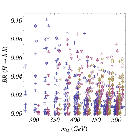
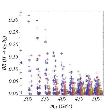
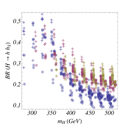
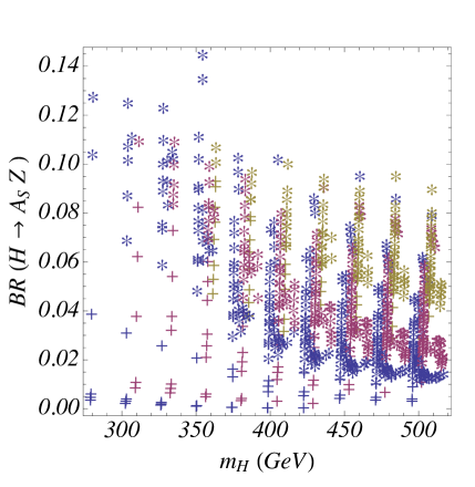
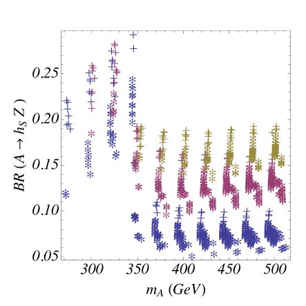
Figs. 10 and 11 show the branching ratio for the decay of the heaviest CP-even Higgs boson into lighter bosons. We observe that these branching ratios are appreciably large for values of the heaviest Higgs boson masses smaller than 350 GeV, for which the decay into top-quark pairs is forbidden, and remain significant for larger value of $m_{A}$, particularly for the largest values of $\tan\beta$ considered. In particular, the decay of $H$ into a pair of non-identical lighter CP-even Higgs bosons is the most important one. In Figs. 10 and 11 we differentiate between the cases in which the lightest CP-even Higgs boson is identified with the SM-like Higgs boson with mass 125 GeV, represented by snowflakes, from the case in which the lightest CP-even Higgs boson is singlet-like (hence with mass below 125 GeV), represented by crosses. We clearly see from Fig. 10 that the decay of $H\to hh$ is suppressed, being at most of order of 10% as a result of the proximity to alignment.

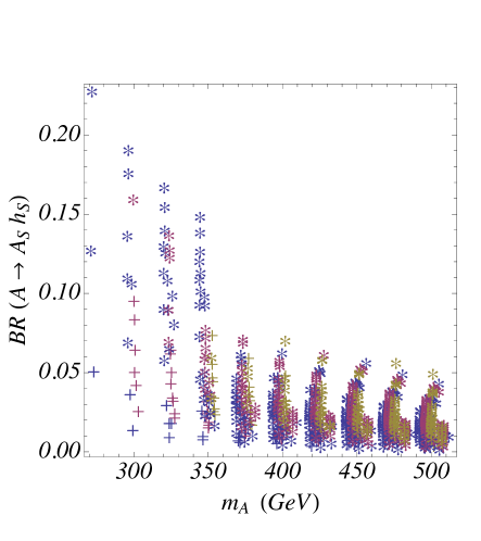
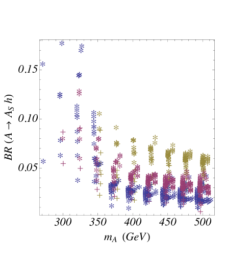
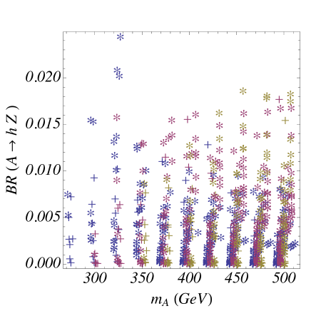
Similarly, in Figs. 12 and 13 we exhibit the branching ratios of the decay of the heaviest CP-odd Higgs boson into the lighter CP-odd and CP-even Higgs bosons, and the branching ratio of its decay into a CP-even Higgs boson and a $Z$ boson. From Fig. 13 we can see that the branching ratio into a $Z$ and the SM-like Higgs boson $h$ is always suppressed. However, the decay of the heavy CP-odd scalar into a $Z$ and $h_{S}$ is unsuppressed and hence may serve as a good discovery channel. This possibility will be addressed later in this Section.

As a result of the approximate alignment condition, $M_{A}\simeq 2|\mu|/s_{2\beta}$ [cf. Eq. (77)], decays of the heavy CP-even and CP-odd Higgs bosons into pairs of charginos and neutralinos are kinematically allowed. In contrast to the case of the MSSM, where heavy gauginos imply a suppression of the coupling of the Higgs bosons to Higgsino pairs, in the NMSSM the coupling $\lambda$ induces a non-negligible coupling to charginos via the singlet component of $H$. Moreover, the coupling $\lambda$ and the self-coupling parameter $\kappa$ induce new decays in the neutralino sector due to the mixing of the singlinos and Higgsinos. Indeed, the singlino mass

$${m_{\tilde{S}}}\simeq\frac{2\kappa}{\lambda}\mu$$ (101)

is constrained to be below the Higgsino mass $\mu$ due to the condition of perturbative consistency up to the Planck scale (see Fig. 2), implying that the decays

$$H,A\to\chi^{0,\pm}_{i}\chi^{0,\mp}_{j}$$ (102)

are likely to have sizable rates in the region of parameters under consideration.

(a)

(b)

Figure 14: Branching ratio of the decay of the heaviest CP-even (left panel) and CP-odd (right panel) Higgs bosons into charginos and neutralinos. Blue, red and yellow represent values of $\tan\beta=2$, 2.5 and 3, respectively.

(a)

(b)

Figure 15: Branching ratio of the decay of the heaviest CP-even Higgs boson (left panel) and the heaviest CP-odd Higgs boson (right panel) into pairs of top quarks. Blue, red and yellow represent values of $\tan\beta=2$, 2.5 and 3, respectively.

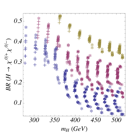
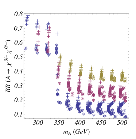
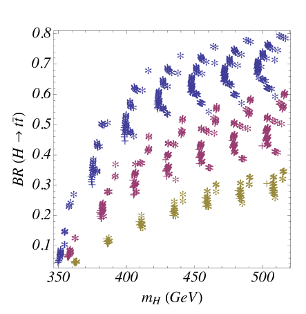
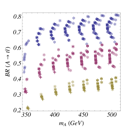
Fig. 14 illustrates that the heavy Higgs bosons $H$ and $A$ have sizable decay branching ratios into charginos and neutralinos. These branching ratios become more prominent for larger values of $\tan\beta$ and for masses below 350 GeV where the decays into top quarks are suppressed.

For completeness, we present the branching ratio of the heaviest CP-even and CP-odd Higgs bosons into top quarks in Fig. 15. As expected, this branching ratio tends to be significant for masses larger than 350 GeV and becomes particularly important at low values of $\tan\beta$, for which the couplings of the heaviest non-SM-like Higgs bosons to the top quark are enhanced. In spite of being close to the alignment limit, this branching ratio is always significantly lower than 1, due to the decays of the Higgs bosons to final states consisting of the lighter Higgs bosons and chargino and/or neutralino pairs, as noted above.

(a)

(b)

Figure 16: Branching ratio of the lightest non-SM-like CP-even Higgs boson into bottom quarks (left panel) and pair of $W$ gauge bosons (right panel). Blue, red and yellow represent values of $\tan\beta=2$, 2.5 and 3, respectively.

Indeed, apart from the decays into top-quark pairs, whose observability demands a good top reconstruction method and is quite challenging Craig:2015jba ; Hajer:2015gka , the heaviest Higgs bosons exhibit prominent branching ratios into lighter Higgs bosons (as in the case of generic 2HDMs Coleppa:2014hxa ). Moreover, in light of the large gluon fusion $A/H$ production cross sections, the heavy Higgs decays into charginos and neutralinos are also relevant and yield production rates that are of the same order of magnitude as the chargino/neutralino Drell-Yan production cross sections. Unfortunately, the subsequent decays of the charginos into $W/Z$ and missing energy renders these search modes challenging.

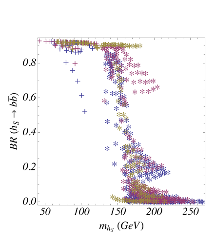
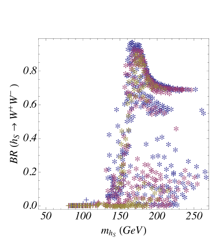
In order to ascertain the constraints on the heavy non-SM-like Higgs bosons arising from their decays into the lightest Higgs bosons, one must analyze the decay branching ratios of $h_{S}$ and $A_{S}$. Since these particles are singlet-like, their couplings are controlled via the mixing with the doublet states. As shown in Fig. 7, the CP-even singlet state has small mixing with the SM-like Higgs boson, $\kappa^{h_{S}}_{\rm SM}=-\eta^{\prime}$, which is small and can be no larger than 0.3. On the other hand, the mixing with the non-SM doublet component $\kappa^{h_{S}}_{\rm NSM}$ is small but non-vanishing. Therefore, as shown in Fig. 16, the bottom quark decays are clearly dominant for masses below 130 GeV, while the $WW$ and eventually $ZZ$ decay branching ratios may become dominant for masses above 130 GeV, depending on the proximity to alignment. For mass values above about 150 GeV, decays into two CP-odd singlet-like Higgs bosons open up for certain regions of parameter space. The singlet-like CP-odd Higgs boson has dominant decay into bottom quark pairs for masses up to about 200 GeV, whereas decays into $Zh_{S}$ and into neutralinos may open up for slightly heavier masses.

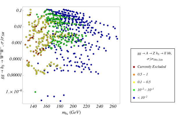
Based on the study of the non-SM-like Higgs boson branching ratios presented above we will now discuss the main search channels which may lead to discovery of the additional scalar states at the LHC. In Fig. 17 we present the 8 TeV production cross sections of the heaviest CP-odd scalar $A$, decaying into a $Z$ and a $h_{S}$ in the $m_{A}$ – $m_{h_{S}}$ plane. The cross sections presented in the left panel of Fig. 17 take into account the decay branching ratios of $Z\to\ell\ell$ and $h_{S}\to b\bar{b}$, since these final states provide excellent search modes at the LHC.

(a)

(b)

Figure 17: The production cross section times branching ratio (left), and the ratio of the observed limit to the production cross section times branching ratio (right) of the decay of the heaviest CP-odd Higgs boson into a $Z$ and a CP-even Higgs boson as a function of the heaviest CP-odd and the singlet like CP-even Higgs boson masses. The cross sections are computed for LHC processes with $\sqrt{s}$ = 8 TeV, and the branching ratio includes the subsequent decay of the Z boson into di-leptons and $h_{S}$ into a bottom quark pair.

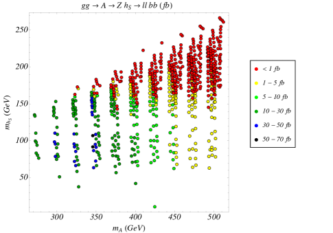
The CMS experiment has already performed searches for scalar resonances decaying into a $Z$ and lighter scalar resonance using 8 TeV data CMS:2015mba . In the right panel of Fig. 17 we have used the CMS ROOT files to compare the limits extracted from these searches with the predictions of the scenario considered here.

We observe that although this mode fails at present to probe a large fraction of the NMSSM Higgs parameter space, the current limit is close to the expected cross section for values of $m_{h_{S}}\stackrel{{\scriptstyle<}}{{{}_{\sim}}}130$ GeV. Hence, $A\to Zh_{S}\to(\ell\ell)(b\bar{b})$ provides a very promising channel for non-SM-like Higgs boson searches in the next run of the LHC. It is also clear from Fig. 17 that for values of the $h_{S}$ mass above 130 GeV, where its decay branching ratio into bottom quarks becomes small, the $A\to Zh_{S}$ search channel becomes less efficient. However, in this case the decay modes into weak gauge bosons may become relevant, and searches for $h_{S}\to WW^{(*)}/ZZ^{(*)}$ may provide an excellent complementary probe.

(a)

Figure 18: The production cross section times branching ratio of the decay of the second heaviest CP-even Higgs into pairs of W, showing the ratio of the observed limit for the heaviest CP-odd Higgs boson into a $Z$ and a CP-even Higgs bosons.

(a)

Figure 19: Ratio of the observed limit to the production cross section times Branching ratio of the decay of the heaviest CP-even Higgs boson into a $Z$ and the lightest CP-odd Higgs bosons.

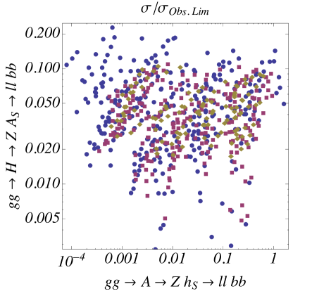
As discussed in Section II, searches for heavy scalar resonances decaying to $WW^{(*)}$ have been performed at the LHC and already constrain the signal strength in the channel $gg\rightarrow h_{S}\to WW^{(*)}$ to be less than 10% of the signal strength from a SM Higgs boson of the same mass. Since the suppression of the decay branching ratio of $h_{S}$ into bottom quarks is in part caused by the increase of the branching ratio into $W$ pairs, it is interesting to investigate the correlation between the search for heavy CP-odd Higgs bosons decaying into $h_{S}Z$ in the $(b\bar{b})(\ell\ell)$ channel and the search for the mainly singlet CP-even Higgs $h_{S}$ decaying into $WW^{(*)}$. To exhibit the complementarity between the two channels, we also show in Fig. 18 the ratios of the event rates for the heavy CP-odd scalar decaying to $h_{S}Z$, with the same colors used in the right panel of Fig. 17. We observe that a large fraction of the parameter space that is difficult to probe in the $A\to Zh_{S}\to(\ell\ell)(b\bar{b})$ channel becomes viable in the search for $gg\to h_{S}\to WW^{(*)}$. There is a small region where searches in both channels become difficult. This is the region where $h_{S}$ has a small coupling to the top quark, thereby suppressing its production cross section, or where the singlet CP-odd scalar mass $m_{A_{S}}$ is small and the decay $h_{S}\to A_{S}A_{S}$ may be allowed. In the latter case, we may use the decay channel $H\to ZA_{S}$ instead.

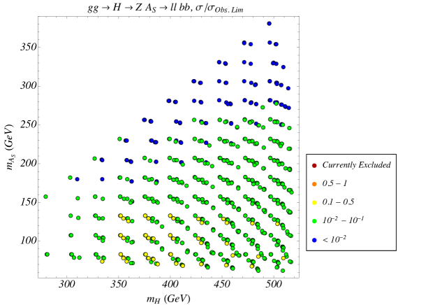
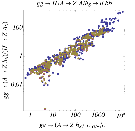
In Fig. 19 we display the ratio of the observed limit to the production cross section of a heavy CP-even Higgs boson $H$ decaying into $H\to ZA_{S}$, with $Z\to\ell\ell$ and $A_{S}\to b\bar{b}$. Due to the somewhat smaller production of $H$ as compared to $A$, there is no point in the NMSSM Higgs parameter space that can be probed at the 8 TeV run of the LHC in this channel. However, for low values of the $A_{S}$ mass, the LHC will become increasingly sensitive to searches in this channel. Moreover, in Fig. 20 we observe the correlation between this ratio and the same ratio for the $A\to Zh_{S}\to(\ell\ell)(b\bar{b})$ channel. The left panel of this figure shows that there is a complementarity in the LHC sensitivity in these two search channels. The right panel shows that an increase of the sensitivity in these two channels by two orders of magnitude would serve to test the full parameter space.

(a)

(b)

Figure 20: Correlation between the ratio of the observed limit to the production cross sections of $A\to Zh_{S}$ and $H\to ZA_{S}$.

(a)

Figure 21: Production cross section times branching ratio of the decay of the heaviest CP-even Higgs boson into $h$ and $h_{S}$, with $h$ decaying into $b\bar{b}$ and $h_{S}$ decaying into $WW$.

(a)

Figure 22: Production cross section times Branching ratio of the decay of the heaviest CP-even Higgs boson into $h$ and $h_{S}$, with both $h$ and $h_{S}$ decaying into $b\bar{b}$.

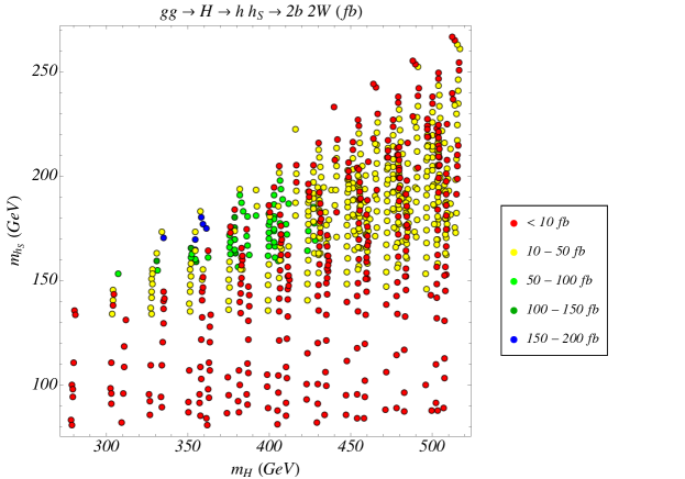
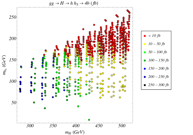
Finally, we consider the decays of the heavy CP-even Higgs bosons into two lighter CP-even scalars, which as shown in Figs. 10 and 11 become prominent in a large region of parameter space. Due to the large size of the branching ratio, it is instructive to focus on the decays of the heavy Higgs bosons into $hh_{S}$. This is shown in Figs. 21 and 22, where we display the 8 TeV LHC cross section of these channels assuming that the SM-like Higgs decays into a pair of bottom quarks and $h_{S}$ decays into $WW^{(*)}$ and bottom pairs, respectively. We see that the cross sections are sizable, of orders of tens or hundreds of fb, and there is a large complementarity between the $bbWW$ and 4$b$ search channels, associated with the significant size of the corresponding $h_{S}$ decay branching ratios.

Most aspects of the NMSSM Higgs phenomenology outlined above can be illustrated by choosing specific benchmarks points in the NMSSM Higgs parameter space. In Appendix D, we present three particular NMSSM benchmarks that illustrate the most important features of the Higgs phenomenology considered in this Section.

V Conclusions

In this paper, we have studied the conditions for the presence of a SM-like Higgs boson in models containing two Higgs doublets and an additional complex singlet scalar. In this so-called alignment limit, one of the neutral Higgs fields approximately points in the same direction in field space as the doublet scalar vacuum expectation value. The main focus of this work is the $\boldsymbol{\mathbb{Z}_{3}}$ invariant NMSSM, which provides a predictive framework in which the interactions of scalars and fermions are well defined. Moreover, in this model the SM-like Higgs mass receives additional tree-level contributions with respect to the MSSM and the Higgsino mass parameter $\mu$ arises from the vacuum expectation value of the singlet field.

The condition of alignment is naturally obtained for the same values of the singlet-doublet coupling, $\lambda\simeq 0.65$, that leads to a relevant contribution to the SM-like Higgs mass at low values of $\tan\beta$, while maintaining the perturbative consistency of the theory up to the Planck scale. Consequently, the stops can be light, inducing only a moderate contribution to the SM-like Higgs mass via radiative loop corrections.

Moreover, the condition of perturbative consistency of the theory up to the Planck scale implies small values of the singlet self-coupling $\kappa$. The mixing of the SM-like Higgs boson with the singlet is reduced and alignment is obtained for values of the mass parameter $M_{A}$ not far from $2|\mu|/s_{2\beta}$. For these values of $M_{A}$, $\kappa$ and $\mu$, the constraints coming from current Higgs boson measurements are satisfied, and the spectrum of the theory in the Higgs sector may be obtained as a function of $A_{\kappa}$, which controls the masses of the CP-even and CP-odd singlet components.

We have shown that for values of $M_{A}\lesssim 500$ GeV, the entire Higgs and Higgsino spectra is accessible at the LHC. Two of the most important probes of this scenario are the searches for heavy scalar resonances, decaying into lighter scalar resonances and a $Z$, as well as the searches for resonances in the $WW$ and $ZZ$ channels. Moreover, the search for scalar resonances decaying into two lighter scalars is also important (with the exception of the decay into $hh$ which tends to be suppressed). Thus it is very important to expand these searches into final states in which at least one of the two light scalars has a mass different from $m_{h}=125$ GeV. We have presented detailed studies of the Higgs phenomenology and considered three benchmarks that capture the dominant features discussed. A comprehensive study of the discovery prospects of these benchmark points at the upcoming LHC Run 2 will be treated in future work.

Appendix A The Higgs scalar potential in the Higgs basis

It is convenient to rewrite the NMSSM Higgs potential [cf. Eqs. (51)–(53)] in terms of the Higgs basis fields $H_{1}$ and $H_{2}$ [defined in Eq. (41)] and the singlet field $S$,

$$\mathcal{V} = Y_{1}H_{1}^{\dagger}H_{1}+Y_{2}H_{2}^{\dagger}H_{2}+[Y_{3}H_{1}^{\dagger}H_{2}+{\rm h.c.}]+Y_{4}S^{\dagger}S$$

$$+\bigl{[}C_{1}H_{1}^{\dagger}H_{1}S+C_{2}H_{2}^{\dagger}H_{2}S+C_{3}H_{1}^{\dagger}H_{2}S+C_{4}H_{2}^{\dagger}H_{1}S+C_{5}(S^{\dagger}S)S+C_{6}S^{3}+{\rm h.c.}\bigr{]}$$

$$+\tfrac{1}{2}Z_{1}(H_{1}^{\dagger}H_{1})^{2}+\tfrac{1}{2}Z_{2}(H_{2}^{\dagger}H_{2})^{2}+Z_{3}(H_{1}^{\dagger}H_{1})(H_{2}^{\dagger}H_{2})+Z_{4}(H_{1}^{\dagger}H_{2})(H_{2}^{\dagger}H_{1})$$

$$\qquad\qquad+\left\{\tfrac{1}{2}Z_{5}(H_{1}^{\dagger}H_{2})^{2}+\big{[}Z_{6}(H_{1}^{\dagger}H_{1})+Z_{7}(H_{2}^{\dagger}H_{2})\big{]}H_{1}^{\dagger}H_{2}+{\rm h.c.}\right\}$$

$$+S^{\dagger}S\bigl{[}Z_{s1}H_{1}^{\dagger}H_{1}+Z_{s2}H_{2}^{\dagger}H_{2}+(Z_{s3}H_{1}^{\dagger}H_{2}+{\rm h.c.})+Z_{s4}S^{\dagger}S\bigr{]}$$

$$+\left\{Z_{s5}H_{1}^{\dagger}H_{1}S^{2}+Z_{s6}H_{2}^{\dagger}H_{2}S^{2}+Z_{s7}H_{1}^{\dagger}H_{2}S^{2}+Z_{s8}H_{2}^{\dagger}H_{1}S^{2}+Z_{s9}S^{\dagger}S\,S^{2}+Z_{s10}S^{4}+{\rm h.c.}\right\}\!.$$

Assuming a CP-invariant Higgs potential and vacuum, all scalar potential coefficients can be taken real after an appropriate rephasing of $H_{2}$. At the minimum of the Higgs potential, $\langle H_{1}^{0}\rangle=v/\sqrt{2}$ and $\langle S\rangle=v_{s}$ (with all other vevs equal to zero), and

$$Y_{1} = -\tfrac{1}{2}Z_{1}v^{2}-2C_{1}v_{s}-(Z_{s1}+2Z_{s5})v_{s}^{2}\,,$$ (104)

$$Y_{3} = -\tfrac{1}{2}Z_{6}v^{2}-(C_{3}+C_{4})v_{s}-(Z_{s3}+Z_{s7}+Z_{s8})v_{s}^{2}\,,$$ (105)

$$Y_{4} = -\tfrac{1}{2}C_{1}\frac{v^{2}}{v_{s}}-3(C_{5}+C_{6})v_{s}-\tfrac{1}{2}(Z_{s1}+2Z_{s5})v^{2}-2Z_{s4}v_{s}^{2}-4(Z_{s9}+Z_{s10})v_{s}^{2}\,.$$ (106)

The charged Higgs mass is given by

$$m_{H^{\pm}}^{2}=M_{A}^{2}-\tfrac{1}{2}(Z_{4}-Z_{5})v^{2}\,,$$ (107)

where the squared-mass parameter $M_{A}^{2}$ is defined by:

$$M_{A}^{2}=Y_{2}+\tfrac{1}{2}(Z_{3}+Z_{4}-Z_{5})v^{2}+2C_{2}v_{s}+(Z_{s2}+2Z_{s6})v_{s}^{2}\,.$$ (108)

The CP-even squared-mass matrix is obtained from Eq. (A) by eliminating $Y_{1}$, $Y_{3}$ and $Y_{4}$,

$$\mathcal{M}^{2}_{S}=\begin{pmatrix}Z_{1}v^{2}&\quad Z_{6}v^{2}&\quad\sqrt{2}\,v\bigl{[}C_{1}+(Z_{s1}+2Z_{s5})v_{s}\bigr{]}\\[10.0pt] &\quad M_{A}^{2}+Z_{5}v^{2}&\quad\displaystyle\frac{v}{\sqrt{2}}\biggl{[}C_{3}+C_{4}+2(Z_{s3}+Z_{s7}+Z_{s8})v_{s}\biggr{]}\\[10.0pt] &&\quad-C_{1}\displaystyle\frac{v^{2}}{2v_{s}}+3(C_{5}+C_{6})v_{s}+4(Z_{s4}+2Z_{s9}+2Z_{s10})v_{s}^{2}\end{pmatrix},$$ (109)

where the omitted elements below the diagonal are fixed since $\mathcal{M}_{S}^{2}$ is a symmetric matrix. Likewise, we can compute the CP-odd squared-mass matrix,

$$\mathcal{M}^{2}_{P}=\begin{pmatrix}M_{A}^{2}&\quad-\displaystyle\frac{v}{\sqrt{2}}\bigl{[}C_{3}-C_{4}+2(Z_{s7}-Z_{s8})v_{s}\bigr{]}\\[10.0pt] &\qquad\quad-C_{1}\displaystyle\frac{v^{2}}{2v_{s}}-(C_{5}+9C_{6})v_{s}-2Z_{s5}v^{2}-4(Z_{s9}+4Z_{s10})v_{s}^{2}\end{pmatrix},$$ (110)

where the omitted matrix element is fixed since $\mathcal{M}_{P}^{2}$ is a symmetric matrix. Comparing the scalar potential $\mathcal{V}$ with Eqs. (51)–(53), we obtain the coefficients of the quadratic terms,

$$Y_{1} = m^{2}_{H_{d}}c_{\beta}^{2}+m^{2}_{H_{u}}s_{\beta}^{2}\,,$$ (111)

$$Y_{2} = m^{2}_{H_{d}}s_{\beta}^{2}+m^{2}_{H_{u}}c_{\beta}^{2}\,,$$ (112)

$$Y_{3} = \tfrac{1}{2}(m^{2}_{H_{u}}-m^{2}_{H_{d}})s_{2\beta}\,,$$ (113)

$$Y_{4} = m_{S}^{2}\,,$$ (114)

the coefficients of the cubic terms [after employing Eqs. (54) and (58)],

$$C_{1} = -C_{2}=\lambda c_{\beta}s_{\beta}\left(\frac{\kappa\mu}{\lambda}-\frac{M_{A}^{2}}{\mu}c_{\beta}s_{\beta}\right)\,,$$ (115)

$$C_{3} = \lambda c_{\beta}^{2}\left(\frac{\kappa\mu}{\lambda}-\frac{M_{A}^{2}}{\mu}c_{\beta}s_{\beta}\right)\,,$$ (116)

$$C_{4} = -\lambda s_{\beta}^{2}\left(\frac{\kappa\mu}{\lambda}-\frac{M_{A}^{2}}{\mu}c_{\beta}s_{\beta}\right)\,,$$ (117)

$$C_{5} = 0\,,$$ (118)

$$C_{6} = \tfrac{1}{3}\kappa A_{\kappa}\,,$$ (119)

and the coefficients of the quartic terms,

$$Z_{1} = Z_{2}=-\tfrac{1}{2}\bigl{[}\lambda^{2}-\tfrac{1}{2}(g^{2}+g^{\prime\,2})\bigr{]}c^{2}_{2\beta}+\tfrac{1}{2}\lambda^{2}\,,$$ (120)

$$Z_{3} = -\tfrac{1}{2}\bigl{[}\lambda^{2}-\tfrac{1}{2}(g^{2}+g^{\prime\,2})\bigr{]}s^{2}_{2\beta}+\tfrac{1}{4}(g^{2}-g^{\prime\,2})\,,$$ (121)

$$Z_{4} = -\tfrac{1}{2}\bigl{[}\lambda^{2}-\tfrac{1}{2}(g^{2}+g^{\prime\,2})\bigr{]}s^{2}_{2\beta}-\tfrac{1}{2}g^{2}+\lambda^{2}\,,$$ (122)

$$Z_{5} = -\tfrac{1}{2}\bigl{[}\lambda^{2}-\tfrac{1}{2}(g^{2}+g^{\prime\,2})\bigr{]}s^{2}_{2\beta}\,,$$ (123)

$$Z_{6} = -Z_{7}=\tfrac{1}{2}\bigl{[}\lambda^{2}-\tfrac{1}{2}(g^{2}+g^{\prime\,2})\bigr{]}s_{2\beta}c_{2\beta}\,,$$ (124)

$$Z_{s1} = Z_{s2}=\lambda^{2}\,,$$ (125)

$$Z_{s4} = \kappa^{2}\,,$$ (126)

$$Z_{s5} = -Z_{s6}=-\tfrac{1}{2}\kappa\lambda s_{2\beta}\,,$$ (127)

$$Z_{s7} = \kappa\lambda s^{2}_{\beta}\,,$$ (128)

$$Z_{s8} = -\kappa\lambda c^{2}_{\beta}\,,$$ (129)

$$Z_{s3} = Z_{s9}=Z_{s10}=0\,.$$ (130)

Note that whereas $Y_{1}$, $Y_{3}$ and $Y_{4}$ are determined from the Higgs potential minimum conditions [Eqs. (104)–(106)], $Y_{2}$ in generic two-doublet/one-singlet models is a free parameter. However, in the $\mathbb{Z}_{3}$-symmetric NMSSM Higgs sector, there is no bare $H_{u}\cdot H_{d}$ term in Eq. (53). Consequently, $Y_{2}$ is no longer an independent parameter. Indeed, Eqs. (111) and (113) yield

$$Y_{2}=Y_{1}+\frac{2c_{2\beta}}{s_{2\beta}}\,Y_{3}\,.$$ (131)

Inserting the results of Eqs. (104) and (105) then yields

$$Y_{2}=-\tfrac{1}{2}Z_{1}v^{2}-2C_{1}v_{s}-(Z_{s1}+2Z_{s5})v_{s}^{2}-\frac{2c_{2\beta}}{s_{2\beta}}\biggl{[}\tfrac{1}{2}Z_{6}v^{2}+(C_{3}+C_{4})v_{s}+(Z_{s3}+Z_{s7}+Z_{s8})v_{s}^{2}\biggr{]}\,.$$ (132)

Inserting this result into Eq. (108) ,

$$M_{A}^{2} = -\tfrac{1}{2}\left(Z_{1}-Z_{3}-Z_{4}+Z_{5}+\frac{2c_{2\beta}}{s_{2\beta}}Z_{6}\right)v^{2}+2\left[C_{2}-C_{1}-\frac{c_{2\beta}}{s_{2\beta}}(C_{3}+C_{4})\right]v_{s}$$ (133)

$$\qquad-\left[Z_{s1}-Z_{s2}+2\biggl{(}Z_{s5}-Z_{s6}+\frac{c_{2\beta}}{s_{2\beta}}(Z_{s3}+Z_{s7}+Z_{s8})\biggr{)}\right]v_{s}^{2}\,.$$

Using the results of this Appendix, one can check that Eq. (133) then reduces to the simple expression given in Eq. (58).

All the results above correspond to tree-level results. Including the leading $\mathcal{O}(h_{t}^{4})$ loop corrections, the $Z_{i}$ are modified as follows:

$$\!\!\!\!\!\!\!\!\!\!\!Z_{1}v^{2} = (m_{Z}^{2}-\tfrac{1}{2}\lambda^{2}v^{2})c^{2}_{2\beta}+\tfrac{1}{2}\lambda^{2}v^{2}+\frac{3v^{2}s_{\beta}^{4}h_{t}^{4}}{8\pi^{2}}\left[\ln\left(\frac{M_{S}^{2}}{m_{t}^{2}}\right)+\frac{X_{t}^{2}}{M_{S}^{2}}\left(1-\frac{X_{t}^{2}}{12M_{S}^{2}}\right)\right],$$ (134)

$$\!\!\!\!\!\!\!\!\!\!\!Z_{2}v^{2} = (m_{Z}^{2}-\tfrac{1}{2}\lambda^{2}v^{2})c^{2}_{2\beta}+\tfrac{1}{2}\lambda^{2}v^{2}+\frac{3v^{2}c_{\beta}^{4}h_{t}^{4}}{8\pi^{2}}\left[\ln\left(\frac{M_{S}^{2}}{m_{t}^{2}}\right)+\frac{Y_{t}^{2}}{M_{S}^{2}}\left(1-\frac{Y_{t}^{2}}{12M_{S}^{2}}\right)\right],$$ (135)

$$\!\!\!\!\!\!\!\!\!\!\!Z_{3}v^{2} = \tfrac{1}{4}(g^{2}-g^{\prime\,2})v^{2}+s_{2\beta}^{2}\biggl{\{}m_{Z}^{2}-\tfrac{1}{2}\lambda^{2}v^{2}+\frac{3v^{2}h_{t}^{4}}{32\pi^{2}}\left[\ln\left(\frac{M_{S}^{2}}{m_{t}^{2}}\right)+\frac{(X_{t}+Y_{t})^{2}}{4M_{S}^{2}}-\frac{X_{t}^{2}Y_{t}^{2}}{12M_{S}^{4}}\right]\biggr{\}},$$

$$Z_{4}v^{2} = (\lambda^{2}-\tfrac{1}{2}g^{2})v^{2}+s_{2\beta}^{2}\left\{m_{Z}^{2}-\tfrac{1}{2}\lambda^{2}v^{2}+\frac{3v^{2}h_{t}^{4}}{32\pi^{2}}\left[\ln\left(\frac{M_{S}^{2}}{m_{t}^{2}}\right)+\frac{(X_{t}+Y_{t})^{2}}{4M_{S}^{2}}-\frac{X_{t}^{2}Y_{t}^{2}}{12M_{S}^{4}}\right]\right\},$$

$$Z_{5}v^{2} = s_{2\beta}^{2}\left\{m_{Z}^{2}-\tfrac{1}{2}\lambda^{2}v^{2}+\frac{3v^{2}h_{t}^{4}}{32\pi^{2}}\left[\ln\left(\frac{M_{S}^{2}}{m_{t}^{2}}\right)+\frac{X_{t}Y_{t}}{M_{S}^{2}}\left(1-\frac{X_{t}Y_{t}}{12M_{S}^{2}}\right)\right]\right\},$$ (138)

$$\!\!\!\!\!\!\!\!\!\!\!Z_{6}v^{2} = -s_{2\beta}\left\{(m_{Z}^{2}-\tfrac{1}{2}\lambda^{2}v^{2})c_{2\beta}-\frac{3v^{2}s_{\beta}^{2}h_{t}^{4}}{16\pi^{2}}\biggl{[}\ln\left(\frac{M_{S}^{2}}{m_{t}^{2}}\right)+\frac{X_{t}(X_{t}+Y_{t})}{2M_{S}^{2}}-\frac{X_{t}^{3}Y_{t}}{12M_{S}^{4}}\biggr{]}\right\},$$ (139)

$$\!\!\!\!\!\!\!\!\!\!\!Z_{7}v^{2} = s_{2\beta}\left\{(m_{Z}^{2}-\tfrac{1}{2}\lambda^{2}v^{2})c_{2\beta}+\frac{3v^{2}c_{\beta}^{2}h_{t}^{4}}{16\pi^{2}}\biggl{[}\ln\left(\frac{M_{S}^{2}}{m_{t}^{2}}\right)+\frac{Y_{t}(X_{t}+Y_{t})}{2M_{S}^{2}}-\frac{X_{t}Y_{t}^{3}}{12M_{S}^{4}}\biggr{]}\right\}.$$ (140)

Appendix B Components of the Mass Eigenstates

We present here generic expressions for the components of the CP-even Higgs mass eigenstates in terms of the mass eigenvalues and the elements of the CP-even Higgs squared-mass matrix. The interaction eigenstates and the mass eigenstates are related by

$$\left(\begin{array}[]{c}h\\ H\\ h_{S}\end{array}\right)=\left(\begin{array}[]{ccc}\kappa^{h}_{\rm SM}&\kappa^{h}_{\rm NSM}&\kappa^{h}_{\rm S}\\ \kappa^{H}_{\rm SM}&\kappa^{H}_{\rm NSM}&\kappa^{H}_{\rm S}\\ \kappa^{h_{S}}_{\rm SM}&\kappa^{h_{S}}_{\rm NSM}&\kappa^{h_{S}}_{\rm S}\end{array}\right)\left(\begin{array}[]{c}H^{\rm SM}\\ H^{\rm NSM}\\ H^{\rm S}\end{array}\right)\ .$$ (141)

For the Higgs mass eigenstate $h$,

$$\frac{\kappa_{\rm NSM}^{h}}{\kappa_{\rm SM}^{h}} = -\frac{\mathcal{M}^{2}_{12}(m_{h}^{2}-\mathcal{M}^{2}_{33})+\mathcal{M}^{2}_{13}\mathcal{M}^{2}_{23}}{\mathcal{M}_{23}^{4}+(\mathcal{M}^{2}_{22}-m_{h}^{2})(m_{h}^{2}-\mathcal{M}^{2}_{33})}\,,$$ (142)

$$\frac{\kappa_{\rm S}^{h}}{\kappa_{\rm SM}^{h}} = \frac{\mathcal{M}^{2}_{13}(\mathcal{M}^{2}_{22}-m_{h}^{2})-\mathcal{M}^{2}_{12}\mathcal{M}^{2}_{23}}{\mathcal{M}^{4}_{23}+(\mathcal{M}^{2}_{22}-m_{h}^{2})(m_{h}^{2}-\mathcal{M}^{2}_{33})}\,.$$ (143)

For the Higgs mass eigenstate $H$,

$$\frac{\kappa_{SM}^{H}}{\kappa_{\rm NSM}^{H}} = -\frac{\mathcal{M}^{2}_{12}(m_{H}^{2}-\mathcal{M}^{2}_{33})+\mathcal{M}^{2}_{13}\mathcal{M}^{2}_{23}}{M_{13}^{4}+(\mathcal{M}^{2}_{11}-m_{H}^{2})(m_{H}^{2}-\mathcal{M}^{2}_{33})}\,,$$ (144)

$$\frac{\kappa_{S}^{H}}{\kappa_{\rm NSM}^{H}} = \frac{\mathcal{M}^{2}_{23}(\mathcal{M}^{2}_{11}-m_{H}^{2})-\mathcal{M}^{2}_{12}\mathcal{M}^{2}_{13}}{\mathcal{M}^{4}_{13}+(\mathcal{M}^{2}_{11}-m_{H}^{2})(m_{H}^{2}-\mathcal{M}^{2}_{33})}\,.$$ (145)

For the Higgs mass eigenstate $h_{S}$,

$$\frac{\kappa_{\rm SM}^{h_{S}}}{\kappa_{\rm S}^{h_{S}}} = -\frac{\mathcal{M}^{2}_{13}(m_{h_{S}}^{2}-\mathcal{M}^{2}_{22})+\mathcal{M}^{2}_{12}\mathcal{M}^{2}_{23}}{M_{12}^{4}+(\mathcal{M}^{2}_{22}-m_{h_{S}}^{2})(m_{h_{S}}^{2}-\mathcal{M}^{2}_{11})}\,,$$ (146)

$$\frac{\kappa_{\rm NSM}^{h_{S}}}{\kappa_{\rm S}^{h_{S}}} = \frac{\mathcal{M}^{2}_{23}(\mathcal{M}^{2}_{11}-m_{h_{S}}^{2})-\mathcal{M}^{2}_{12}\mathcal{M}^{2}_{13}}{M_{12}^{4}+(\mathcal{M}^{2}_{22}-m_{h_{S}}^{2})(m_{h_{S}}^{2}-\mathcal{M}^{2}_{11})}\,.$$ (147)

Appendix C Analytic Expressions for the Higgs Couplings

C.1 Trilinear Higgs Couplings

In Table 1 we present the tree-level Higgs trilinear couplings in terms of Higgs-basis scalar fields. The second column of Table 1 displays the corresponding coefficients derived from the Higgs potential, Eq. (A), and the third column of Table 1 evaluates these coefficients in the $\mathbb{Z}_{3}$-invariant NMSSM using the results of Eqs. (115)–(130). The corresponding Feynman rules are obtained by multiplication by a symmetry factor $-i\,n!$, where $n$ is the number of identical bosons that are associated with the trilinear coupling. From Table 1 we see that the coefficient of the Higgs trilinear couplings $H^{\rm NSM}H^{\rm SM}H^{\rm SM}$ and $H^{\rm S}H^{\rm SM}H^{\rm SM}$ are proportional to $\mathcal{M}^{2}_{12}$ and $\mathcal{M}^{2}_{13}$, Eq. (LABEL:eq:CPMM), respectively, and approach zero in the alignment limit.

	coefficient in $\mathcal{V}$ [Eq. (A)]	$\mathbb{Z}_{3}$-invariant NMSSM
$H^{\rm SM}H^{\rm SM}H^{\rm SM}$	$\tfrac{1}{2}vZ_{1}$	$\tfrac{1}{8}v\bigl{[}2\lambda^{2}s^{2}_{2\beta}+(g^{2}+g^{\prime\,2})c^{2}_{2\beta}\bigr{]}$
$H^{\rm SM}H^{\rm SM}H^{\rm NSM}$	$\tfrac{3}{2}vZ_{6}$	$\tfrac{3}{4}v(\lambda^{2}-g^{2}-g^{\prime\,2})s_{2\beta}c_{2\beta}$
$H^{\rm SM}H^{\rm NSM}H^{\rm NSM}$	$\tfrac{1}{2}v(Z_{3}+Z_{4}+Z_{5})$	$\tfrac{1}{8}\bigl{[}2\lambda^{2}+(2\lambda^{2}-g^{2}-g^{\prime\,2})(1-3s^{2}_{2\beta})\bigr{]}$
$H^{\rm NSM}H^{\rm NSM}H^{\rm NSM}$	$\tfrac{1}{2}vZ_{7}$	$-\tfrac{1}{4}v(\lambda^{2}-g^{2}-g^{\prime\,2})s_{2\beta}c_{2\beta}$
$H^{\rm SM}H^{\rm SM}H^{\rm S}$	$\bigl{[}C_{1}+v_{s}(Z_{s1}+2Z_{s5})\bigr{]}/\sqrt{2}$	$\frac{\lambda\mu}{\sqrt{2}}\left[1-\tfrac{1}{2}s_{2\beta}\left(\frac{\kappa}{\lambda}+\frac{M_{A}^{2}}{2\mu^{2}}s_{2\beta}\right)\right]$
$H^{\rm SM}H^{\rm NSM}H^{\rm S}$	$\bigl{[}C_{3}+C_{4}+2v_{s}(Z_{s3}+Z_{s7}+Z_{s8})\bigr{]}/\sqrt{2}$	$-\frac{\lambda\mu c_{2\beta}}{\sqrt{2}}\left(\frac{\kappa}{\lambda}+\frac{M_{A}^{2}}{2\mu^{2}}s_{2\beta}\right)$
$H^{\rm NSM}H^{\rm NSM}H^{\rm S}$	$\bigl{[}C_{2}+v_{s}(Z_{s2}+2Z_{s6})\bigr{]}/\sqrt{2}$	$\frac{\lambda\mu}{\sqrt{2}}\left[1+\tfrac{1}{2}s_{2\beta}\left(\frac{\kappa}{\lambda}+\frac{M_{A}^{2}}{2\mu^{2}}s_{2\beta}\right)\right]$
$H^{\rm SM}H^{\rm S}H^{\rm S}$	$\tfrac{1}{2}v(Z_{s1}+2Z_{s5})$	$\tfrac{1}{2}v\lambda(\lambda-\kappa s_{2\beta})$
$H^{\rm NSM}H^{\rm S}H^{\rm S}$	$\tfrac{1}{2}v(Z_{s3}+Z_{s7}+Z_{s8})$	$-\tfrac{1}{2}v\kappa\lambda c_{2\beta}$
$H^{\rm S}H^{\rm S}H^{\rm S}$	$\bigl{[}C_{5}+C_{6}+2v_{s}(Z_{s4}+2Z_{s9}+2Z_{s10})\bigr{]}/\sqrt{2}$	$\tfrac{\kappa}{3\sqrt{2}}(A_{\kappa}+6\frac{\kappa\mu}{\lambda})$
$H^{\rm SM}A^{\rm NSM}A^{\rm NSM}$	$\tfrac{1}{2}v(Z_{3}+Z_{4}-Z_{5})$	$\tfrac{1}{4}v\bigl{[}\lambda^{2}+\bigl{(}\lambda^{2}-\tfrac{1}{2}(g^{2}+g^{\prime\,2})\bigr{)}c_{2\beta}^{2}\bigr{]}$
$H^{\rm NSM}A^{\rm NSM}A^{\rm NSM}$	$\tfrac{1}{2}vZ_{7}$	$-\tfrac{1}{4}v\bigl{[}\lambda^{2}-\tfrac{1}{2}(g^{2}+g^{\prime\,2})\bigr{]}s_{2\beta}c_{2\beta}$
$H^{\rm S}A^{\rm NSM}A^{\rm NSM}$	$\bigl{[}C_{2}+v_{s}(Z_{s2}+2Z_{s6})\bigr{]}/\sqrt{2}$	$\frac{\lambda\mu}{\sqrt{2}}\left[1+\tfrac{1}{2}s_{2\beta}\left(\frac{\kappa}{\lambda}+\frac{M_{A}^{2}}{2\mu^{2}}s_{2\beta}\right)\right]$
$H^{\rm SM}A^{\rm NSM}A^{\rm S}$	$\bigl{[}C_{4}-C_{3}-2v_{s}(Z_{s7}-Z_{s8})\bigr{]}$	$\frac{\lambda\mu}{\sqrt{2}}\left(\frac{M_{A}^{2}}{2\mu^{2}}s_{2\beta}-3\frac{\kappa}{\lambda}\right)$
$H^{\rm NSM}A^{\rm NSM}A^{\rm S}$	0	0
$H^{\rm S}A^{\rm NSM}A^{\rm S}$	$v(Z_{s8}-Z_{s7})$	$-\kappa\lambda v$
$H^{\rm SM}A^{\rm S}A^{\rm S}$	$\tfrac{1}{2}v(Z_{s1}-2Z_{s5})$	$\tfrac{1}{2}v\lambda(\lambda+\kappa s_{2\beta})$
$H^{\rm NSM}A^{\rm S}A^{\rm S}$	$\tfrac{1}{2}v(Z_{s3}-Z_{s7}-Z_{s8})$	$\tfrac{1}{2}v\kappa\lambda c_{2\beta}$
$H^{\rm S}A^{\rm S}A^{\rm S}$	$\bigl{[}C_{5}-3C_{6}+2v_{s}(Z_{s4}+6Z_{s10})\bigr{]}/\sqrt{2}$	$-\kappa(A_{\kappa}-2\frac{\kappa\mu}{\lambda})/\sqrt{2}$
$H^{\rm SM}H^{+}H^{-}$	$vZ_{3}$	$-\tfrac{1}{2}\bigl{[}\lambda^{2}-\tfrac{1}{2}(g^{2}+g^{\prime\,2})\bigr{]}s^{2}_{2\beta}+\tfrac{1}{4}(g^{2}-g^{\prime\,2})$
$H^{\rm NSM}H^{+}H^{-}$	$vZ_{7}$	$-\tfrac{1}{2}\bigl{[}\lambda^{2}-\tfrac{1}{2}(g^{2}+g^{\prime\,2})\bigr{]}s_{2\beta}c_{2\beta}$
$H^{\rm S}H^{+}H^{-}$	$\sqrt{2}\bigl{[}C_{2}+v_{s}(Z_{s2}+2Z_{s6})\bigr{]}$	$\sqrt{2}\,\lambda\mu\left[1+\tfrac{1}{2}s_{2\beta}\left(\frac{\kappa}{\lambda}+\frac{M_{A}^{2}}{2\mu^{2}}s_{2\beta}\right)\right]$

Table 1: Tree-level trilinear scalar interactions.

We can also include the effects of the dominant contributions to the one-loop radiative corrections to the trilinear scalar interactions by employing the leading $\mathcal{O}(h_{t}^{4})$ corrections given in Eqs. (134)–(140). These corrections modify the trilinear Higgs couplings shown in Table 2. The results presented in Table 2 have been obtained as follows. First, we work in the approximation that $m_{h}^{2}\simeq Z_{1}v^{2}$. We then use Eq. (134) to solve for $\ln(M_{S}^{2}/m_{t}^{2})$ in terms of $m_{h}^{2}$, $m_{Z}^{2}$, $\lambda$, and $X_{t}$. The resulting expression is then used in Eqs. (135)–(140) to eliminate the logarithmic terms. Using the resulting expressions for the $Z_{i}$ to evaluate the trilinear couplings in Table 1, we obtain the results shown in Table 2 after dropping the additional corrections proportional to $(X_{t}-Y_{t})/M_{S}$. Note in particular that $m_{h}$, which appears in the trilinear Higgs couplings shown in Table 2, is the radiatively-corrected Higgs mass in the NMSSM, which we set equal to 125 GeV. That is, the leading radiative corrections to the Higgs trilinear couplings have been absorbed in the definition of $m_{h}$.

	$2v\,\times$ trilinear Higgs coupling of the $\mathbb{Z}_{3}$-invariant NMSSM
$H^{\rm SM}H^{\rm SM}H^{\rm SM}$	$m_{h}^{2}$
$H^{\rm SM}H^{\rm SM}H^{\rm NSM}$	$3s^{-1}_{\beta}\left(m_{h}^{2}c_{\beta}-m_{Z}^{2}c_{2\beta}c_{\beta}-\tfrac{1}{2}\lambda^{2}v^{2}s_{2\beta}s_{\beta}\right)$
$H^{\rm SM}H^{\rm NSM}H^{\rm NSM}$	$3s^{-2}_{\beta}\left[m_{h}^{2}c^{2}_{\beta}-m_{Z}^{2}(c^{2}_{2\beta}-\tfrac{2}{3}s^{2}_{\beta})-\lambda^{2}v^{2}s^{2}_{\beta}(c_{2\beta}+\tfrac{2}{3})\right]$
$H^{\rm NSM}H^{\rm NSM}H^{\rm NSM}$	$s_{\beta}^{-3}\left[m_{h}^{2}c_{\beta}^{3}+m_{Z}^{2}c_{2\beta}c_{\beta}(2s^{2}_{\beta}-c^{2}_{\beta})-\tfrac{1}{2}\lambda^{2}v^{2}s_{2\beta}s_{\beta}(2c^{2}_{\beta}-s^{2}_{\beta})\right]$
$H^{\rm SM}A^{\rm NSM}A^{\rm NSM}$	$s^{-2}_{\beta}\left(m_{h}^{2}c_{\beta}^{2}-m_{Z}^{2}c^{2}_{2\beta}-\lambda^{2}v^{2}c_{2\beta}s_{\beta}^{2}\right)$
$H^{\rm NSM}A^{\rm NSM}A^{\rm NSM}$	$s_{\beta}^{-3}\left[m_{h}^{2}c_{\beta}^{3}+m_{Z}^{2}c_{2\beta}c_{\beta}(2s^{2}_{\beta}-c^{2}_{\beta})-\tfrac{1}{2}\lambda^{2}v^{2}s_{2\beta}s_{\beta}(2c^{2}_{\beta}-s^{2}_{\beta})\right]$
$H^{+}H^{-}H^{\rm SM}$	$4m_{W}^{2}+2s^{-2}_{\beta}\left(m_{h}^{2}c_{\beta}^{2}-m_{Z}^{2}c^{2}_{2\beta}-\tfrac{1}{2}\lambda^{2}v^{2}s^{2}_{2\beta}\right)$
$H^{+}H^{-}H^{\rm NSM}$	$2s_{\beta}^{-3}\left[m_{h}^{2}c_{\beta}^{3}+m_{Z}^{2}c_{2\beta}c_{\beta}(2s^{2}_{\beta}-c^{2}_{\beta})-\tfrac{1}{2}\lambda^{2}v^{2}s_{2\beta}s_{\beta}(2c^{2}_{\beta}-s^{2}_{\beta})\right]$

Table 2: Approximate one-loop corrected trilinear scalar interactions.

C.2 Coupling of neutral Higgs bosons to neutral gauge bosons

In contrast to the coupling of a CP-even Higgs boson to pairs of gauge bosons, which is present only for $H^{\rm SM}$, the derivative couplings of pairs of neutral scalars to the neutral gauge boson are governed by the gauge interactions of the non-SM Higgs doublet. That is,

$$g_{H^{\rm NSM}A^{\rm NSM}Z}=\tfrac{1}{2}i\sqrt{g_{1}^{2}+g_{2}^{2}}\left(p-p^{\prime}\right)^{\mu}$$ (148)

where $p$ and $p^{\prime}$ are the incoming momentum of $H^{\rm NSM}$ and $A^{\rm NSM}$, respectively and $ig_{H^{\rm NSM}A^{\rm NSM}Z}$ is the corresponding Feynman rule for the $H^{\rm NSM}A^{\rm NSM}Z$ vertex.

C.3 Couplings of the mass eigenstate Higgs fields

It is instructive to derive the expressions for the couplings among the different mass eigenstate Higgs bosons in the exact alignment limit. In light of Eq. (79), we shall also assume that the mixing between the doublet and singlet CP-even scalar fields are small. In the notation introduced in Section II.2, we take $\epsilon_{1}=\epsilon_{2}=\eta^{\prime}=0$ (corresponding to the exact alignment limit) and $|\eta|\ll 1$, in which case $m_{h}^{2}=Z_{1}v^{2}$ and Eq. (82) reduces to

$$\left(\begin{array}[]{c}h\\ H\\ h_{S}\end{array}\right)\simeq\left(\begin{array}[]{ccc}1&\phantom{-}0&\phantom{-}0\\ 0&-1&-\eta\\ 0&\ -\eta&\phantom{-}1\end{array}\right)\left(\begin{array}[]{c}H^{\rm SM}\\ H^{\rm NSM}\\ H^{\rm S}\end{array}\right)\,.$$ (149)

Similarly, we shall assume that the mixing between the doublet and singlet CP-odd scalar fields are small. In this approximation,

$$\left(\begin{array}[]{c}A\\ A_{S}\end{array}\right)\simeq\left(\begin{array}[]{ccc}\phantom{-}1&\phantom{-}\xi\\ -\xi&\phantom{-}1\end{array}\right)\left(\begin{array}[]{c}A^{\rm NSM}\\ A^{\rm S}\end{array}\right)\,,$$ (150)

where $|\xi|\ll 1$. The interactions of the scalar mass-eigenstates are given in Table 3, where terms quadratic (and higher order) in $\eta$ and $\xi$ have been neglected. The trilinear Higgs interactions are expressed in terms of the coefficients, $C_{ijk}$ that appear in Table 1, where the subscripts $i$, $j$, $k$ label the Higgs basis scalar fields. In particular, $C_{H^{\rm NSM}A^{\rm NSM}A^{\rm S}}=0$ for the scalar potential given in Eq. (A), and $C_{H^{\rm SM}H^{\rm SM}H^{NSM}}=C_{H^{\rm SM}H^{\rm SM}H^{S}}=0$ in the exact alignment limit. These relations have been implemented in obtaining Table 3.

The Higgs interactions with a single $Z$ boson are expressed in terms of the $H^{\rm NSM}A^{\rm NSM}Z$ interaction, denoted by $G$ in Table 3. The corresponding Feynman rules, denoted by $-ig_{abc}$ (where $a$, $b$ and $c$ label the Higgs mass eigenstate fields), are obtained by multiplying the entries of the second column of Table 3 by $-i\,n!$, where $n$ is the number of identical boson fields appearing in the interaction term.

vertex	term in the interaction Lagrangian
$hhh$	$C_{H^{\rm SM}H^{\rm SM}H^{\rm SM}}$
$hhH$	$0$
$hHH$	$C_{H^{\rm SM}H^{\rm NSM}H^{\rm NSM}}+2\eta C_{H^{\rm SM}H^{\rm NSM}H^{S}}$
$HHH$	$-C_{H^{\rm NSM}H^{\rm NSM}H^{\rm NSM}}-3\eta C_{H^{\rm NSM}H^{\rm NSM}H^{S}}$
$hhh_{S}$	$0$
$hh_{S}H$	$-C_{H^{\rm SM}H^{\rm NSM}H^{S}}-\eta C_{H^{\rm SM}H^{S}H^{S}}+\eta C_{H^{\rm SM}H^{\rm NSM}H^{\rm NSM}}$
$HHh_{S}$	$\phantom{xxxx}C_{H^{\rm NSM}H^{\rm NSM}H^{\rm S}}-\eta C_{H^{\rm NSM}H^{\rm NSM}H^{\rm NSM}}+2\eta C_{H^{\rm NSM}H^{\rm S}H^{\rm S}}\phantom{xxxx}$
$hh_{S}h_{S}$	$C_{H^{\rm SM}H^{\rm S}H^{\rm S}}-2\eta C_{H^{\rm SM}H^{\rm NSM}H^{\rm S}}$
$Hh_{S}h_{S}$	$-C_{H^{\rm NSM}H^{\rm S}H^{\rm S}}+2\ \eta\ C_{H^{\rm NSM}H^{\rm NSM}H^{\rm S}}-\eta\ C_{H^{\rm S}H^{\rm S}H^{\rm S}}$
$h_{S}h_{S}h_{S}$	$C_{H^{\rm S}H^{\rm S}H^{\rm S}}+3\eta C_{H^{\rm NSM}H^{\rm S}H^{\rm S}}$
$hAA$	$C_{H^{\rm SM}A^{\rm NSM}A^{\rm NSM}}+2\xi C_{H^{\rm SM}A^{\rm NSM}A^{\rm S}}$
$HAA$	$-C_{H^{\rm NSM}A^{\rm NSM}A^{\rm NSM}}-\eta C_{H^{\rm S}A^{\rm NSM}A^{\rm NSM}}$
$h_{S}AA$	$C_{H^{\rm S}A^{\rm NSM}A^{\rm NSM}}-\eta C_{H^{\rm NSM}A^{\rm NSM}A^{\rm NSM}}+2\xi C_{H^{\rm S}A^{\rm NSM}A^{\rm S}}$
$hAA_{S}$	$C_{H^{\rm SM}A^{\rm NSM}A^{\rm S}}-\xi C_{H^{\rm SM}A^{\rm NSM}A^{\rm NSM}}+\xi C_{H^{\rm SM}A^{\rm S}A^{\rm S}}$
$HAA_{S}$	$-\eta C_{H^{\rm S}A^{\rm NSM}A^{\rm S}}-\xi C_{H^{\rm NSM}A^{\rm S}A^{\rm S}}+\xi C_{H^{\rm NSM}A^{\rm NSM}A^{\rm NSM}}$
$h_{S}AA_{S}$	$C_{H^{\rm S}A^{\rm NSM}A^{\rm S}}+\xi C_{H^{\rm S}A^{\rm S}A^{\rm S}}-\xi C_{H^{\rm S}A^{\rm NSM}A^{\rm NSM}}$
$hA_{S}A_{S}$	$C_{H^{\rm SM}A^{\rm S}A^{\rm S}}-2\xi C_{H^{\rm SM}A^{\rm NSM}A^{\rm S}}$
$HA_{S}A_{S}$	$-C_{H^{\rm NSM}A^{\rm S}A^{\rm S}}-\eta C_{H^{\rm S}A^{\rm S}A^{\rm S}}$
$h_{S}A_{S}A_{S}$	$C_{H^{\rm S}A^{\rm S}A^{\rm S}}-\eta C_{H^{\rm NSM}A^{\rm S}A^{\rm S}}-2\xi g_{H^{\rm S}A^{\rm NSM}A^{\rm S}}$
$hH^{+}H^{-}$	$C_{H^{\rm SM}H^{+}H^{-}}$
$HH^{+}H^{-}$	$-C_{H^{\rm NSM}H^{+}H^{-}}-\eta C_{H^{\rm S}H^{+}H^{-}}$
$h_{S}H^{+}H^{-}$	$C_{H^{\rm S}H^{+}H^{-}}-\eta C_{H^{\rm NSM}H^{+}H^{-}}$
$AhZ$	$0$
$AHZ$	$G$
$Ah_{S}Z$	$-\eta G$
$A_{S}hZ$	$0$
$A_{S}HZ$	$-\xi G$
$A_{S}h_{S}Z$	$0$

Table 3: Interactions of the mass-eigenstate scalars in the alignment limit. The coefficients $C$ are given in Table 1 and $G$ is the $A^{\rm NSM}H^{\rm NSM}Z$ interaction coefficient.

Appendix D Benchmarks

In this section we present three benchmarks that illustrate the most important features of the Higgs phenomenology considered in Section IV. Except for the third generation squarks, the gluinos, the sleptons and the squarks are all kept at the TeV scale and decouple from the low energy phenomenology at the electroweak scale. The value of $\lambda=0.65$ is chosen to obtain alignment and preserve the perturbativity up to the Planck scale. The relevant parameters are given in Table 4.

	Benchmark 1a	Benchmark 1b	Benchmark 2	Benchmark 3
$\tan\beta$	2.1	2.1	2.5	2.5
$M_{1}$(GeV)	122	200	135	-400
$M_{2}$(GeV)	-500	600	$-300$	$-800$
$A_{t}$(GeV)	$-650$	-750	$-900$	$-1400$
$m_{Q_{3}}$(GeV)	700	700	700	800
$m_{U_{3}}$(GeV)	340	340	700	800
$\kappa$	0.3	0.3	0.3	0.3
$A_{\lambda}$(GeV)	210	210	350	350
$A_{\kappa}$(GeV)	$-90$	-75	$-270.$	-100
$\mu$(GeV)	122	120	174.	200.

Table 4: Parameters for the three different benchmarks.

The Higgs and stop spectra obtained by NMSSMTools using these input parameters are displayed in Table 5, and the chargino and neutralino masses are given in Table 6. The production cross sections for the neutral Higgs scalars at the LHC are presented in Table 7, while some relevant processes, including the Higgs decay branching ratios are summarized in Table 8. In what follows we will focus on the low-energy phenomenology and discuss the salient features of each benchmark scenario.

	Benchmark 1a	Benchmark 1b	Benchmark 2	Benchmark 3
$m_{h}$(GeV)	124.5	125.3	125.4	124.5
$m_{h_{S}}$(GeV)	93.4	94.5	72.54	160.3
$m_{H}$(GeV)	301.0	293.0	470.37	513.1
$m_{A_{S}}$(GeV)	175.4	167.7	280.16	208.4
$m_{A}$(GeV)	295.3	286.4	466.26	507.6
$m_{H^{+}}$(GeV)	280.6	272.0	456.5	500.0
$m_{\tilde{t}_{1}}$(GeV)	272.7	255.3	625.77	693.6
$m_{\tilde{t}_{2}}$(GeV)	722.3	726.7	826.26	966.6

Table 5: Higgs and stop masses in the three benchmarks.

	Benchmark 1a	Benchmark 1b	Benchmark 2	Benchmark 3
$m_{\chi^{0}_{1}}$(GeV)	77.0	77.7	106.6	170.7
$m_{\chi^{0}_{2}}$(GeV)	145.5	164.4	171.3	226.9
$m_{\chi^{0}_{3}}$(GeV)	164.0	169.2	200.1	255.1
$m_{\chi^{0}_{4}}$(GeV)	187.8	216.9	237.1	401.4
$m_{\chi^{0}_{5}}$(GeV)	519.5	619.5	327.4	812.4
$m_{\chi^{\pm}_{1}}$(GeV)	130.4	110.9	179.9	207.2
$m_{\chi^{\pm}_{1}}$(GeV)	519.5	619.4	327.3	812.4

Table 6: Electroweakino masses in the three benchmarks.

	Benchmark 1a	Benchmark 1b	Benchmark 2	Benchmark 3
$\sigma(gg\to h\to b\bar{b})/\sigma_{SM}$	0.85	0.93	1.00	0.80
$\sigma(gg\to h\to VV)/\sigma_{SM}$	1.28	1.16	1.01	1.12
$\sigma(gg\to h_{S}\to VV)/\sigma_{SM}$	$1.1\times 10^{-3}$	8.1 $10^{-4}$	–	0.05
$\sigma(VV\to h_{S}\to b\bar{b})/\sigma_{SM}$	0.054	0.036	6.2 $10^{-4}$	0.8
$\sigma(gg\to H)$(pb) ( 8 TeV)	1.20	1.28	0.31	0.21
$\sigma(gg\to H)$(pb) (14 TeV)	3.83	4.14	1.28	0.89
$\sigma(gg\to A)$(pb) (8 TeV)	2.18	2.21	0.57	0.35
$\sigma(gg\to A)$(pb) ( 14 TeV)	7.10	7.11	2.28	1.48

Table 7: Relevant production cross sections for the three benchmarks.

x
Benchmark scenarios 1a and 1b

	Benchmark 1a	Benchmark 1b	Benchmark 2	Benchmark 3
BR($b\to s\gamma$) $\times$ $10^{4}$	3.76	3.57	$3.68$	$3.59$
$\Omega h^{2}$	0.119	0.013	0.128	0.011
$\sigma_{SI}$(pb) $\times$ $10^{10}$	2.41 $10^{-2}$	3.17	11.0	0.02
BR($h_{S}\to b\bar{b}$)	0.91	0.91	0.91	0.57
BR($h_{S}\to W^{+}W^{-}$)	7.5 $\times 10^{-5}$	8 $10^{-5}$	$--$	0.23
BR($H\to t\bar{t}$)	$-$	$--$	0.39	0.52
BR($H\to hh_{S}$)	0.47	0.39	0.24	0.16
BR($H\to\chi_{i}^{0}\chi_{j}^{0})$	0.33	0.31	0.26	0.20
BR($H\to\chi_{1}^{+}\chi_{1}^{-}$)	0.009	0.14	0.008	0.001
BR($A\to t\bar{t}$)	$-$	$--$	0.53	0.59
BR($A\to Zh_{S}$)	0.36	0.21	0.16	0.14
BR($A\to\chi_{i}^{0}\chi_{j}^{0}$)	0.51	0.47	0.31	0.18
BR($A\to\chi_{1}^{+}\chi_{1}^{-}$)	0.001	0.19	0.01	0.0005
BR($A_{S}\to b\bar{b}$)	0.01	0.005	0.007	0.87
BR($A_{S}\to\chi_{1}^{0}\chi_{1}^{0}$)	0.99	0.99	0.96	$-$
BR($H^{+}\to t\bar{b}$)	0.73	0.73	0.55	0.62
BR($H^{+}\to W^{+}h_{S}$)	0.15	0.15	0.18	0.15
BR($H^{+}\to\chi_{1}^{+}\chi_{i}^{0}$)	0.10	0.11	0.24	0.18

Table 8: Relevant processes in the three benchmarks.

The first two Benchmarks, 1a and 1b have similar spectra but differ slightly in the degree of alignment of the SM-like Higgs with the singlet state and the value of the electroweak gaugino masses. Benchmark 1a has a dark matter relic density consistent with the observed one and a spin independent direct detection scattering cross section significantly below the current experimental bound, while Benchmark 1b has a heavier gaugino spectrum and a relic density an order of magnitude below the observed one. In both of these benchmarks the stop spectrum has been fixed to obtain the observed 125 GeV Higgs mass and the $b\to s\gamma$ rate, keeping the non-SM Higgs bosons light. In addition, Benchmark 1a and 1b have the following properties:

Higgs Searches: The second lightest Higgs boson $h$ behaves like the observed (SM-like) Higgs boson with mass 125 GeV due to alignment at low $\tan\beta$. The mostly doublet non-SM Higgs boson masses $m_{A}$ and $m_{H}$ are around 300 GeV, and hence the neutral Higgs boson decays into top quark pairs are forbidden, while the charged Higgs boson decays mostly into top and bottom quarks, with BR$(H^{\pm}\rightarrow tb)~{}\approx 0.7$. Both neutral Higgs bosons decay into electroweakinos with combined branching ratios of about 40% or larger, whereas the charged Higgs decay into electroweakinos is only at the 10% level. The other relevant decays of the neutral CP-even Higgs boson are into $hh_{S}$ (40%) and $h_{S}h_{S}$ (10%).

The CP-odd scalar $A$ has a sizable decay with a branching ratio of about 36% (20%) into $h_{S}Z$ in scenario 1a (1b) and the charged Higgs decays into $Wh_{S}$ with a 15% branching ratio. The increase in the branching ratio of the decay of $A\to h_{S}Z$ in scenario 1a compared to 1b is due to the decrease of the decay into charginos. Such an increase makes the $A$ signatures compatible with an excess observed by CMS in the $bb\ell\ell$ channel CMS:2015mba for masses of the heavier and lighter Higgs states consistent with the one assumed in Benchmark 1a. On the other hand, the decay of $H$ and $A$ into charginos in Benchmark 1b leads to a chargino production cross section of the same order as the one coming from Drell Yan processes and makes it possible to test this scenario in the search for charginos at the Run 2 of the LHC.

The mainly singlet CP-even Higgs boson $h_{S}$ decays dominantly into bottom quark pairs, while the mainly singlet CP-odd Higgs bosons $A_{S}$ decays overwhelmingly into a pair of the lightest neutralinos. The small increase of the misalignment in Benchmark 1a compared to 1b implies a possible contribution to the LEP $e^{+}e^{-}\to Z^{*}\to Zh_{S}$ cross section of the order of 5.5%, consistent with a small excess observed at LEP in this channel for this range of masses.

It therefore follows that the most promising discovery modes for these two benchmarks at the LHC are in the topologies $2\ell 2b$, 4$b$ or $2b2W$ arising mainly from the gluon fusion production of $H$ and $A$ with subsequent decays $A\rightarrow Zh_{S}$ and $H\rightarrow hh_{S}$, respectively, as discussed in section IV, as well as in the search for chargino pair production.

Stop searches: In both Benchmark 1a and 1b, the mass of one of the stops is approximately equal to the sum of the mass of the top and the lightest neutralino. This motivates the search for stops at the LHC in this challenging region of parameters. The other stop, mainly $\widetilde{t}_{L}$, is about 725 GeV in mass and can be searched for in decays into top or bottom quarks and electroweakinos. The lightest sbottom is also about 700 GeV in mass, and can be searched for in several channels at the LHC.

Electroweakino searches: The lightest neutralinos are singlino-Higgsino admixtures, with an additional bino component in Benchmark 1a. Both the second and third lightest neutralinos have a mass gap with respect to the lightest neutralino which is less than $m_{Z}$, and therefore will decay into $Z^{*}\chi^{0}_{1}$. The lightest chargino has a mass of about 110 GeV, and is Higgsino-like. The small mass difference between the lightest chargino and neutralino makes the leptons coming from the chargino decays soft and difficult to detect.

Benchmark scenario 2

Benchmark 2 is more traditional in the sense that the relic density is consistent with the observed one. The spin independent direct detection cross section is below but close to the LUX Akerib:2013tjd experimental bound, and therefore can be soon tested by the next generation of Xenon experiments. In addition, it has the following properties

Higgs searches: The second lightest Higgs boson $h$ behaves like the observed (SM-like) Higgs boson with mass 125 GeV due to alignment at low $\tan\beta$. The lightest, mostly singlet CP-even Higgs boson $h_{S}$ is lighter than the $Z$ boson and decays predominantly to bottom quark pairs. The lightest CP-odd Higgs boson $A_{S}$ has a mass of about 300 GeV and decays predominantly into neutralinos, with a 4% branching ratio into $Zh_{S}$. The non-SM doublet Higgs boson masses $m_{H}$ and $m_{A}$ are about 470 GeV. Consequently, both neutral Higgs bosons have relevant decays into top quark pairs. Given that the charged Higgs boson mass is about 460 GeV, the $b\to s\gamma$ rate is consistent with observations without the need of a light stop. The dominant decays for the heavy neutral CP-even Higgs boson $H$ are: 40% into $t\bar{t}$, 25% into $hh_{S}$ and about 30% into electroweakinos. Similarly, $A$ decays 55% of the time into $t\bar{t}$, 16% into $Zh_{S}$ and about 30% into electroweakinos. The charged Higgs boson decays 55% of the time into $t\bar{b}$, 20% into $Wh_{S}$, and 25% into electroweakinos. Similar to Benchmarks 1a and 1b, the most promising discovery modes for $A$ and $H$ in this benchmark scenario at the LHC are via the topologies $2\ell 2b$, $4b$ or $2b2W$. However the fact that they are heavier and both have significant decays into top quark pairs makes detection more challenging.

Stop searches: Both stops are in the $625$ – $825$ GeV range and decay into many different channels, including bottom–chargino and top–neutralino final states. Their masses can be raised somewhat by lowering the stop mixing, without spoiling the consistency with the observed Higgs mass. The left-handed sbottom masses are of the same order.

Electroweakino searches: Many different electroweakinos are present in the mass range of 100 – 350 GeV. The lightest neutralino mass is about 110 GeV. The second and third lightest neutralinos, as well as the charginos, are about 180 GeV and hence can be looked for in trilepton searches. Since the lightest electroweakinos are Higgsino and singlino like, the cross sections are smaller than for winos Beenakker:1996ed ; Ellwanger:2013rsa . In particular, observe that $\chi^{0}_{2}$ is in the region marginally excluded by CMS for winos, but since it is mostly an admixture of Higgsino and singlino, its production cross section is suppressed with respect to the wino one. Hence there are good prospects to search for some of the electroweakinos efficiently at Run 2 of the LHC.

Benchmark scenario 3

Benchmark 3 presents a scenario where $h_{S}\to WW$ is a relevant search channel at the LHC. The thermal relic density contribution is small, demanding the presence of non-thermal production of the lightest neutralino. The spin independent cross section is an order of magnitude smaller than the current LUX bound. In addition, this scenario has the following properties:

Higgs searches: The lightest Higgs boson $h$ is the observed (SM-like) Higgs boson with mass 125 GeV, while the second lightest CP-even Higgs $h_{S}$ is mostly singlet and has a mass close to the $WW$ threshold, hence decays dominantly into $W^{\pm}$ pairs. The gluon fusion production cross section of $h_{S}$ times its branching ratio into $W^{\pm}$ pairs is about 4$\%$ of the SM cross section for a Higgs boson of the same mass. Hence $h_{S}$ can be efficiently searched for at the current run of the LHC. The main difference between the Higgs phenomenology for Benchmarks 2 and 3 is the exchange of roles between the two lightest mainly singlet Higgs bosons, $h_{S}$ and $A_{S}$, since now $A_{S}$ has a mass of about 130 GeV and decays predominantly in bottom quark pairs. The heavy Higgs boson $H$ decays prominently into top pairs (45$\%$), into two different lightest Higgs bosons, $hh_{S}$ (21$\%$) and into electroweakinos (32$\%$). The CP-odd Higgs boson $A$ has also prominent decays into top pairs (54$\%$), into $Z\;h_{S}$ ($15\%$) and into electroweakinos ($21\%$). Therefore, this benchmark may be tested efficiently at the LHC in the topologies $2\ell 2W$, $2b2W$ or $4W$ through the gluon production of $A$ and $H$ and their subsequent decays into $Zh_{S}$ and $hh_{S}$, respectively.

Stop Searches: The stop and sbottom spectra are similar to the ones in Benchmark 2. Charginos and neutralinos are heavier, but the the third generation squarks may decay into multiple channels and may be searched for efficiently at the Run 2 of LHC.

Electroweakino searches: The lightest electroweakinos are admixtures of singlinos and Higgsinos, with mass gaps that are smaller than the weak gauge boson masses. Hence, searches at the LHC are difficult and will demand high luminosity.

References

- (1) G. Aad et al. [ATLAS Collaboration], Phys. Lett. B 716, 1 (2012) [arXiv:1207.7214 [hep-ex]]; G. Aad et al. [ATLAS Collaboration], Phys. Lett. B 726, 88 (2013) [arXiv:1307.1427 [hep-ex]].
- (2) S. Chatrchyan et al. [CMS Collaboration], Phys. Lett. B 716, 30 (2012) [arXiv:1207.7235 [hep-ex]]; S. Chatrchyan et al. [CMS Collaboration], JHEP 1306, 081 (2013) [arXiv:1303.4571 [hep-ex]].
- (3) H. E. Haber and R. Hempfling, Phys. Rev. Lett. 66, 1815 (1991); Y. Okada, M. Yamaguchi and T. Yanagida, Prog. Theor. Phys. 85, 1 (1991); J. R. Ellis, G. Ridolfi and F. Zwirner, Phys. Lett. B 257, 83 (1991).
- (4) H. E. Haber and R. Hempfling, Phys. Rev. D 48, 4280 (1993) [hep-ph/9307201].
- (5) See e.g., M. Carena, H. E. Haber, S. Heinemeyer, W. Hollik, C. E. M. Wagner and G. Weiglein, Nucl. Phys. B 580, 29 (2000) [hep-ph/0001002]; G. Degrassi, S. Heinemeyer, W. Hollik, P. Slavich and G. Weiglein, Eur. Phys. J. C 28, 133 (2003) [hep-ph/0212020].
- (6) G. F. Giudice and A. Strumia, Nucl. Phys. B 858, 63 (2012) [arXiv:1108.6077 [hep-ph]].
- (7) E. Bagnaschi, G. F. Giudice, P. Slavich and A. Strumia, JHEP 1409, 092 (2014) [arXiv:1407.4081 [hep-ph]].
- (8) P. Draper, G. Lee and C. E. M. Wagner, Phys. Rev. D 89, 055023 (2014) [arXiv:1312.5743 [hep-ph]].
- (9) J. P. Vega and G. Villadoro, JHEP 1507, 159 (2015) [arXiv:1504.05200 [hep-ph]].
- (10) G. Lee and C. E. M. Wagner, arXiv:1508.00576 [hep-ph].
- (11) U. Ellwanger, C. Hugonie and A. M. Teixeira, Phys. Rept. 496, 1 (2010) [arXiv:0910.1785 [hep-ph]].
- (12) J. F. Gunion and H. E. Haber, Phys. Rev. D 67, 075019 (2003) [hep-ph/0207010].
- (13) A. Delgado, G. Nardini and M. Quiros, JHEP 1307, 054 (2013) [arXiv:1303.0800 [hep-ph]].
- (14) N. Craig, J. Galloway and S. Thomas, arXiv:1305.2424 [hep-ph].
- (15) See Chapter 1.3 of D. M. Asner, T. Barklow, C. Calancha, K. Fujii, N. Graf, H. E. Haber, A. Ishikawa and S. Kanemura et al., arXiv:1310.0763 [hep-ph].
- (16) M. Carena, I. Low, N. R. Shah and C. E. M. Wagner, JHEP 1404, 015 (2014) [arXiv:1310.2248 [hep-ph]].
- (17) H. E. Haber, arXiv:1401.0152 [hep-ph].
- (18) P. S. B. Dev and A. Pilaftsis, JHEP 1412, 024 (2014) [arXiv:1408.3405 [hep-ph]]; D. Das and I. Saha, Phys. Rev. D 91, 095024 (2015) [arXiv:1503.02135 [hep-ph]]; P. S. B. Dev and A. Pilaftsis, J. Phys. Conf. Ser. 631, 012030 (2015) [arXiv:1503.09140 [hep-ph]]; J. Bernon, J. F. Gunion, H. E. Haber, Y. Jiang and S. Kraml, Phys. Rev. D 92, 075004 (2015) [arXiv:1507.00933 [hep-ph]]; H. E. Haber and O. Stål, Eur. Phys. J. C 75, 491 (2015) [arXiv:1507.04281 [hep-ph]].
- (19) M. Carena, H. E. Haber, I. Low, N. R. Shah and C. E. M. Wagner, Phys. Rev. D 91, 035003 (2015) [arXiv:1410.4969 [hep-ph]].
- (20) U. Ellwanger, JHEP 1203, 044 (2012) [arXiv:1112.3548 [hep-ph]].
- (21) J. F. Gunion, Y. Jiang and S. Kraml, Phys. Lett. B 710, 454 (2012) [arXiv:1201.0982 [hep-ph]].
- (22) S. F. King, M. Muhlleitner and R. Nevzorov, Nucl. Phys. B 860, 207 (2012) [arXiv:1201.2671 [hep-ph]].
- (23) J. J. Cao, Z. X. Heng, J. M. Yang, Y. M. Zhang and J. Y. Zhu, JHEP 1203, 086 (2012) [arXiv:1202.5821 [hep-ph]].
- (24) D. A. Vasquez, G. Belanger, C. Boehm, J. Da Silva, P. Richardson and C. Wymant, Phys. Rev. D 86, 035023 (2012) [arXiv:1203.3446 [hep-ph]].
- (25) U. Ellwanger and C. Hugonie, Adv. High Energy Phys. 2012, 625389 (2012) [arXiv:1203.5048 [hep-ph]].
- (26) K. Agashe, Y. Cui and R. Franceschini, JHEP 1302, 031 (2013) [arXiv:1209.2115 [hep-ph]].
- (27) K. Kowalska, S. Munir, L. Roszkowski, E. M. Sessolo, S. Trojanowski and Y. L. S. Tsai, Phys. Rev. D 87, 115010 (2013) [arXiv:1211.1693 [hep-ph]].
- (28) S. F. King, M. Mühlleitner, R. Nevzorov and K. Walz, Nucl. Phys. B 870, 323 (2013) [arXiv:1211.5074 [hep-ph]].
- (29) T. Gherghetta, B. von Harling, A. D. Medina and M. A. Schmidt, JHEP 1302, 032 (2013) [arXiv:1212.5243 [hep-ph]].
- (30) R. Barbieri, D. Buttazzo, K. Kannike, F. Sala and A. Tesi, Phys. Rev. D 87, no. 11, 115018 (2013) [arXiv:1304.3670 [hep-ph]].
- (31) M. Badziak, M. Olechowski and S. Pokorski, JHEP 1306, 043 (2013) [arXiv:1304.5437 [hep-ph]].
- (32) U. Ellwanger, JHEP 1308, 077 (2013) [arXiv:1306.5541 [hep-ph]].
- (33) F. Domingo and G. Weiglein, arXiv:1509.07283 [hep-ph].
- (34) S. F. King, M. Mühlleitner, R. Nevzorov and K. Walz, Phys. Rev. D 90, 095014 (2014) [arXiv:1408.1120 [hep-ph]].
- (35) H. Georgi and D. V. Nanopoulos, Phys. Lett. B 82, 95 (1979); J. F. Donoghue and L. F. Li, Phys. Rev. D 19, 945 (1979); L. Lavoura and J. P. Silva, Phys. Rev. D 50, 4619 (1994) [hep-ph/9404276]; L. Lavoura, Phys. Rev. D 50, 7089 (1994) [hep-ph/9405307]; F. J. Botella and J. P. Silva, Phys. Rev. D 51, 3870 (1995) [hep-ph/9411288].
- (36) See Chapter 22 of G. C. Branco, L. Lavoura and J. P. Silva, CP Violation (Oxford University Press, Oxford, UK, 1999).
- (37) J. R. Ellis, J. F. Gunion, H. E. Haber, L. Roszkowski and F. Zwirner, Phys. Rev. D 39, 844 (1989).
- (38) J. F. Gunion, H. E. Haber, G. L. Kane and S. Dawson, The Higgs Hunter’s Guide (Westview Press, Boulder, CO, 2000).
- (39) G. C. Branco, P. M. Ferreira, L. Lavoura, M. N. Rebelo, M. Sher and J. P. Silva, Phys. Rept. 516, 1 (2012) [arXiv:1106.0034 [hep-ph]].
- (40) L. J. Hall and M. B. Wise, Nucl. Phys. B 187, 397 (1981).
- (41) P. Fayet, Nucl. Phys. B 90, 104 (1975); K. Inoue, A. Kakuto, H. Komatsu and S. Takeshita, Prog. Theor. Phys. 67, 1889 (1982); R. A. Flores and M. Sher, Annals Phys. 148, 95 (1983).
- (42) J. F. Gunion and H. E. Haber, Nucl. Phys. B 272, 1 (1986) [Erratum-ibid. B 402, 567 (1993)].
- (43) V. Khachatryan et al. [CMS Collaboration], arXiv:1504.00936 [hep-ex].
- (44) P. M. Ferreira, J. F. Gunion, H. E. Haber and R. Santos, Phys. Rev. D 89, 115003 (2014) [arXiv:1403.4736 [hep-ph]].
- (45) M. Farina, M. Perelstein and B. Shakya, JHEP 1404, 108 (2014) [arXiv:1310.0459 [hep-ph]].
- (46) T. Gherghetta, B. von Harling, A. D. Medina and M. A. Schmidt, JHEP 1404, 180 (2014) [arXiv:1401.8291 [hep-ph]].
- (47) U. Ellwanger and C. Hugonie, Comput. Phys. Commun. 175, 290 (2006) [hep-ph/0508022].
- (48) P. Bechtle, O. Brein, S. Heinemeyer, O. Stål, T. Stefaniak, G. Weiglein and K. E. Williams, Eur. Phys. J. C 74, 2693 (2014) [arXiv:1311.0055 [hep-ph]].
- (49) http://www.th.u-psud.fr/NMHDECAY/nmssmtools.html
- (50) N. Craig, F. D’Eramo, P. Draper, S. Thomas and H. Zhang, JHEP 1506, 137 (2015) [arXiv:1504.04630 [hep-ph]].
- (51) J. Hajer, Y. Y. Li, T. Liu and J. F. H. Shiu, arXiv:1504.07617 [hep-ph].
- (52) B. Coleppa, F. Kling and S. Su, JHEP 1409, 161 (2014) [arXiv:1404.1922 [hep-ph]].
- (53) CMS Collaboration [CMS Collaboration], CMS-PAS-HIG-15-001.
- (54) D. S. Akerib et al. [LUX Collaboration], Phys. Rev. Lett. 112, 091303 (2014) [arXiv:1310.8214 [astro-ph.CO]].
- (55) W. Beenakker, R. Hopker and M. Spira, hep-ph/9611232.
- (56) U. Ellwanger, JHEP 1311, 108 (2013) [arXiv:1309.1665 [hep-ph]].