Nonlinear response and emerging nonequilibrium micro-structures for biased diffusion in confined crowding environments

Abstract

We study analytically the dynamics and the micro-structural changes of a host medium caused by a driven tracer particle moving in a confined, quiescent molecular crowding environment. Imitating typical settings of active micro-rheology experiments, we consider here a minimal model comprising a geometrically confined lattice system – a two-dimensional strip-like or a three-dimensional capillary-like – populated by two types of hard-core particles with stochastic dynamics – a tracer particle driven by a constant external force and bath particles moving completely at random. Resorting to a decoupling scheme, which permits us to go beyond the linear-response approximation (Stokes regime) for arbitrary densities of the lattice gas particles, we determine the force-velocity relation for the tracer particle and the stationary density profiles of the host medium particles around it. These results are validated a posteriori by extensive numerical simulations for a wide range of parameters. Our theoretical analysis reveals two striking features: a) We show that, under certain conditions, the terminal velocity of the driven tracer particle is a nonmonotonic function of the force, so that in some parameter range the differential mobility becomes negative, and b) the biased particle drives the whole system into a nonequilibrium steady-state with a stationary particle density profile past the tracer, which decays exponentially, in sharp contrast with the behavior observed for unbounded lattices, where an algebraic decay is known to take place.

I Introduction

Rheological properties of soft matter systems at the micro-scale can be investigated by studying the motion of an active tracer particle (TP), or some other probe, that can sample length scales typical of the microstructure of the host medium. The study of the system response to a local perturbation is particularly relevant to complex and heterogeneous media, such as glasses, gels, and many biological systems. Experimentally, the microscopic probe can be driven externally by using magnetic or optical tweezers; such an experimental technique, called active micro-rheology, (where the term “active” emphasizes that the tracer is not in equilibrium with the environment but rather induces some micro-structural changes in the host medium), has been successfully applied to probe the micro-rheological properties of a variety of different systems (see, e.g., SM10 ; WP11 for recent reviews), including living cells WMT06 , colloidal suspensions PV14 , soft glassy materials GCOAB08 ; JMCBC12 , and granular media CD10 ; WGZS14 ; GPSV14 ; SGPV15 , to name but a few.

It was realized, in particular, that in all these systems the presence of a boundary and interactions with it, as well as the specific geometry of the sample affect not only the dynamics of the tracer particle but are also relevant for the response properties of the medium. Indeed, the study of driven diffusion in confined geometries BHMST08 , e.g., in micro-channels, where the surface-to-volume ratios are large, opened up a broad front of research, with important applications in several fields, such as, e.g., micro- and nanofluidics MG01 ; SHR08 , hydrodynamics at solid-liquid interfaces JYB06 , reaction-diffusion kinetics BCKMV10 , dynamics of colloids B02 ; GKKRWH08 ; TM08 ; AR11 and polymers G11 , dense liquids LF14 , and crowded systems WHVB12 ; BBCILMOV13 .

In order to characterize the dynamics of the TP, biased by a constant force $F$, and its effect on the host medium, the first goal is to establish the so-called force-velocity relation $V(F)$; namely, the dependence of the stationary velocity $V$ of the probe on the applied force. This characteristic curve depends on the mutual interaction between the tracer and the surrounding medium. In the context of active micro-rheology of colloidal suspensions, different theoretical approaches to relate the tracer dynamics with the structural properties of the host medium have been proposed: in the low density limit, the friction coefficient in the nonlinear response regime can be obtained from a simplified many-body Smoluchowski equation, where the knowledge of the density profile around the tracer is required SB05 ; in the dense limit, a mode-coupling approximation allows one to compute the friction coefficient from the probe’s position correlation function FC02 . A general finding is that $V(F)$ can show non-trivial nonlinear behaviors, such as force-thinning or thickening PV14 ; WS15 .

A second important point in the characterization of the system response is to understand how the motion of the TP perturbs the surrounding medium and whether this perturbation is localized or, on the contrary, is long-ranged. This information is contained in the particle density profiles around the tracer. Due to the driving force acting on the TP, one expects to observe an accumulation of particles in front of it – a “traffic jam”, and a low-density wake, depleted by the bath particles behind it. This traffic jam produces an extra contribution to the frictional force exerted on the TP, resulting in an increased friction BCCMO00 . Clearly, the unperturbed value of the equilibrium particle density should be approached at infinitely large distances from it. Such asymmetric density profiles are observed, for instance, in simulations of colloidal dispersions CB05 ; ZB10 or lattice gases MO10 , in experiments SMF10 , and in glass-forming soft-sphere mixtures WH13 ; DBJ14 . This inhomogeneous spatial distribution of the bath particles induced by the TP and traveling along together with it signifies that the TP drives the whole system out of equilibrium bringing it to a nonequilibrium steady-state. This has important physical consequences, e.g., it can give rise to effective bath- and bias-mediated interactions in the system DLL03 ; MO10 . Quantitatively, an exact calculation of the density profiles around stationary moving tracer particle is impossible, since here one faces a genuine essentially many-body problem and one has to resort to approximate approaches. In particular, for colloidal suspensions important results have been obtained using the dynamic density functional theory PDT03 ; RDKP07 ; TM08 .

Analytical results describing the nonlinear coupling between the TP and the dynamical environment can be obtained within the framework of lattice gases – minimalistic models that are able to reproduce some of the main features of more complex systems. Lattice gas models consist of particles that can jump from one site of the lattice to another, with the only constraint that each site can be occupied at most by one particle (excluded-volume interactions). This physically means that apart from constraining particle dynamics on the lattice, we take into account only the repulsive part of the particle-particle interaction potential. The host medium is represented by bath particles, performing a (symmetric in all directions) random walk among the neighboring lattice sites. The TP is also considered as a mobile hard-core particle, equal in size to the bath particles, but may have a different characteristic jump time and, in active micro-rheology settings, be subjected to a constant external force favoring its jumps in a preferential direction, see Fig. 1, in agreement with the local detailed balance (LDB) LS99 . The model can then be viewed as an asymmetric exclusion process (the so-called ASEP) evolving in a sea of symmetric exclusion processes (SEPs) M15 , and represents a combination of two paradigmatic models for transport phenomena in nonequilibrium statistical mechanics.

Recently, the behavior of $V(F)$ beyond the linear regime in lattice gas models has received great attention, triggered by the observation of the striking phenomenon of negative differential mobility (NDM), namely a nonmonotonic dependence of the TP velocity on the applied force P05 ; JKGC08 ; LF13 ; BBMS13 ; BM14 ; BIOSV14 ; BSV15 . Upon a gradual increase of the force $F$, the velocity grows linearly, as prescribed by the linear response, then approaches a maximal value and further decreases with an increase of $F$. This remarkable “getting more from pushing less” behavior ZPM02 occurs not only in lattice models, but it is observed in several systems, such as nonequilibrium steady states ZPM02 , Brownian motors CM96 ; KMHLT06 , and kinesin models AWV15 . In particular, in the context of kinetically constraint models, NDM has been observed in numerical simulations in JKGC08 ; S08 and related to the heterogeneity and intermittency of the dynamics in the glassy phase JKGC08 . More recently, an analytical theory accounting for NDM in a Lorentz lattice gas, where the TP travels among fixed obstacles, has been presented by Leitmann and Franosch LF13 in the dilute limit (i.e. at linear order in the obstacle density). Later, Basu and Maes BM14 observed via numerical simulations the same phenomenon in a dynamical environment, where obstacles can diffuse with excluded-volume interactions, and related NDM with the “frenetic” contributions appearing in a nonequilibrium fluctuation-dissipation relation LCZ05 ; BMW09 ; LCSZ08 ; BKLM15 ; BM15 . A general analytical approach, accounting for NDM in dynamical environments, and valid for arbitrary density and arbitrary choice of transition rates, has been then proposed and discussed in BIOSV14 , where the trapping effect induced on the TP by the coupling between the density and the characteristic time scale of bath particles, was indicated as the main physical mechanism responsible for the phenomenon. The study of the dependence of NDM on the microscopic dynamical rules has been further investigated by Baiesi and coworkers BSV15 , who stressed that the particular shape of the obstacles and their coupling with the TP can play a central role in determining the effective trapping mechanism.

In this paper we present a general analytical treatment which unifies and extends previous studies, and allows us to compute the force-velocity relation of the TP and the density profiles around it for arbitrary densities and for arbitrary values of the exerted force, in experimentally relevant geometrically-restricted systems – strip-like or capillary-like confinement; namely, for bounded lattices which have an infinite extent in the direction of the applied force and are finite in other directions, perpendicular to the direction of the applied force, see Fig. 2. Our theoretical approach is based on a decoupling of correlation functions of the site occupation variable and can be applied to any choice of the transition rates, including, in particular, the cases studied in the recent literature mentioned above. This approximation has been previously introduced for one-dimensional models in BOMM92 ; BOMR96 ; BCLMO99 and subsequently generalized for higher dimensional infinite lattices in BCMO99 ; BCCMO00 ; BCCMO01 . Here we extend this analysis over an experimentally-relevant, but technically more involved case of dense crowded environments placed in confined, geometrically-restricted systems. As mentioned above, these particular boundary conditions have important applications in many systems and therefore it is worth to study how they influence the system’s response.

Our first main result is the derivation of the analytic expression for the velocity $V(F)$ from the decoupling approximation, valid for any choice of jump probabilities and arbitrary density. The comparison of this result with extensive numerical simulations reveals that the approximation is very accurate in a wide range of parameters. We proceed to show that, in a certain region of the parameter space but not always, the force-velocity relation is a nonmonotonous function, so that when $F$ exceeds a certain value, at which $V$ attains a maximum, the velocity starts to decrease. In this regime, remarkably, the differential mobility becomes negative. Moreover, we study in detail the behaviors arising from two specific choices of the TP jump probabilities, considered recently in LF13 ; BM14 ; BIOSV14 , both satisfying the LDB, but differing in the explicit dependence on $F$ in the directions orthogonal to the force. We derive the phase chart in the parameter space of the model where NDM is expected to occur for both kinds of jump probabilities. Our study unifies and clarifies quantitatively the recent analyses mentioned above, on the role of the microscopic dynamical rules in nonequilibrium systems, driven beyond the linear response regime BIOSV14 ; BSV15 .

The second issue we address concerns the effect of boundary conditions on the density profiles around the TP. In particular, it is unclear in which way such a confinement will influence the emergent nonequilibrium micro-structure of the host medium. On the one hand, in BCCMO01 the computation of the density profiles around a TP in an adsorbed monolayer of hard-core particles showed that, if the particle density in the monolayer is conserved, the approach to the equilibrium density with the distance past the tracer is described by a power-law function footnote1 . On the other hand, it is known BOMR96 ; OBBM that in strictly one-dimensional systems – the so-called single-files, there are no stationary profiles past the driven tracer. The systems we consider here are physically two- (stripes) and three-dimensional (capillaries), but effectively they are quasi-one-dimensional since they are of an infinite extent only in one direction. Therefore, the outcome is a priori not evident. We show that the approach of the local host particles density at large distances past the tracer is exponential, in sharp contrast with the power-law behavior observed in unbounded systems BCCMO01 . More precisely, in the case of strip-like geometry of size $L$, our analytical approach allows us to identify a characteristic length, marking the passage from an initial algebraic decay at short distances to an asymptotic exponential relaxation. This length scale diverges with the size $L$ of the stripe, resulting in a pure algebraic decay for infinite lattices, as expected. Our study reveals that the strong memory effects in the spatial distribution of particles in the wake of the tracer are suppressed by the confining geometry, due to a fast homogenization effect.

The paper is organized as follows. In Section II we describe the model and define the relevant parameters. In Section III we present our results for $V(F)$ in the case of confined geometries and compare the analytical predictions against Monte Carlo numerical simulations. In Section IV we study the phenomenon of NDM and discuss the effects of different microscopic dynamical rules. In Section V we report the analytical results for the density profiles around the tracer for a strip-like geometry and compare them with the case of infinite lattices. Finally, in Section VI we conclude with a brief recapitulation of our results and outline further research. In Appendices A and B, details on the analytical computations for the force-velocity relation and the density profiles, respectively, are provided.

II The model

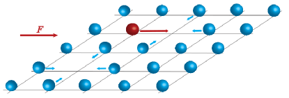
Figure 1: Lattice gas with driven tracer. The hard-core tracer particle (in red) is subjected to an external force $F$ and performs a biased random walk, while the bath particles (in blue) perform nearest-neighbor lattice random walks, constrained by excluded-volume interactions.

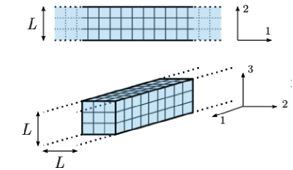
Figure 2: Sketch of strip- and capillary-like confined geometries. The external force is applied along the direction in which the system has an infinite extent.

We consider a $d-$dimensional hyper-cubic lattice with unit lattice spacing, bounded or not, populated by hard-core particles, with total average density $\rho$ (see Fig. 1). The particle dynamics is defined by the following rules: Each bath particle waits an exponentially distributed time with mean $\tau^{*}$ and then selects one of the nearest-neighboring sites with probability $1/2d$. If the chosen site is empty at this time moment, the particle jumps; otherwise, if the target site is occupied, the particle stays at its position. We also introduce a tracer particle, with a different mean waiting time $\tau$, and with jump probabilities in the direction $\nu$ ($\nu\in\{\pm 1,\ldots,\pm d\}$)

$$p_{\nu}=\frac{e^{(\beta/2)\boldsymbol{F}\cdot\boldsymbol{e}_{\nu}}}{\sum_{\mu}e^{(\beta/2)\boldsymbol{F}\cdot\boldsymbol{e}_{\mu}}},$$ (1)

where $\beta$ is the inverse temperature (measured in the units of the Boltzmann constant), $\boldsymbol{e}_{\mu}$ are the $2d$ base vectors of the lattice, and $\boldsymbol{F}\equiv F\boldsymbol{e}_{1}$ is the external force. In the following, we will refer to Eq. (1) as Choice 1. Notice that in this case, in the limit $F\to\infty$, the TP performs a totally directed motion, where only the steps in the field direction are permitted. This situation can be relevant for modeling molecular motors, such as the protein kinesin moving on microtubules BBPZ15 .

Let us stress that the choice in Eq. (1) is not univocal. It coincides with that of Ref. LF13 , but the transition rates in the transverse direction with respect to the field can have different expressions, as considered for instance in JKGC08 ; BM14 . The theoretical treatment proposed in the following is however general and does not rely on a specific form of $p_{\nu}$. In order to illustrate this point, and in order to analyze the effect of different forms of jump probabilities, we will also explicitly consider the case of Ref. BM14 , which, in two dimensions, corresponds to the definition

$$p^{\prime}_{\pm 1}=\frac{1}{2}\frac{e^{\pm\beta F/2}}{e^{\beta F/2}+e^{-\beta F/2}},$$ (2)

and $p^{\prime}_{\pm 2}=1/4$. In this case, the jump probabilities in the directions orthogonal to the force are constant, and we will refer to this expression as Choice 2 in the rest of the paper. Note that both Choice 1 and Choice 2 satisfy the LDB, which guarantees that, at linear order in $F$, the Einstein relation is verified. However, out of equilibrium, or in the nonlinear regime, the explicit dependence of the transition rates on $F$ can have important effects, as we will discuss in detail in Section IV.

III Stationary velocity in confined geometries

In this Section we present an analytical computation of the stationary velocity of the tracer, based on a decoupling approximation.

III.1 General formalism

Let the Boolean variable $\eta(\boldsymbol{R})=\{1,0\}$ denote the instantaneous occupation variable of the site at position $\boldsymbol{R}$ by any of the bath particles, $\eta\equiv\{\eta(\boldsymbol{R})\}$ denote the instantaneous configuration of all such occupation variables and $\boldsymbol{R}_{TP}$ - the instantaneous position of the TP. The evolution of the joint probability $P(\boldsymbol{R}_{TP},\eta;t)$ that at time $t$ the TP is at site $\boldsymbol{R}_{TP}$ with the configuration of obstacles $\eta$, is ruled by the master equation

$$\partial_{t}P(\boldsymbol{R}_{TP},\eta;t)=\frac{1}{2d\tau^{*}}$$ (3)

$$\times \sum_{\mu=1}^{d}\sum_{\boldsymbol{r}\neq\boldsymbol{R}_{TP}-\boldsymbol{e}_{\mu},\boldsymbol{R}_{TP}}[P(\boldsymbol{R}_{TP},\eta^{\boldsymbol{r},\mu};t)-P(\boldsymbol{R}_{TP},\eta;t)]$$

$$+ \frac{1}{\tau}\sum_{\mu=1}^{d}p_{\mu}\{[1-\eta(\boldsymbol{R}_{TP})]P(\boldsymbol{R}_{TP}-\boldsymbol{e}_{\mu},\eta;t)$$

$$- [1-\eta(\boldsymbol{R}_{TP}+\boldsymbol{e}_{\mu})]P(\boldsymbol{R}_{TP},\eta;t)\},$$

where $\eta^{\boldsymbol{r},\mu}$ is the configuration obtained from $\eta$ by exchanging the occupation numbers of sites $\boldsymbol{r}$ and $\boldsymbol{r}+\boldsymbol{e}_{\mu}$. The first term in r.h.s. of the above equation describes the change in $P(\boldsymbol{R}_{TP},\eta;t)$ due to the bath particles jumps, while the second and third lines take into account the TP moves.

Multiplying both sides of the master equation by $(\boldsymbol{R}_{TP}\cdot\boldsymbol{e}_{1})$, summing over all configurations $(\boldsymbol{R}_{TP},\eta)$, and taking the long time limit $t\to\infty$, we obtain the following expression for the TP velocity

$$V=\frac{1}{\tau}\left\{p_{1}\left[1-k(\boldsymbol{e}_{1})\right]-p_{-1}\left[1-k(\boldsymbol{e}_{-1})\right]\right\},$$ (4)

where the function $k({\boldsymbol{\lambda}})$ is the stationary value of $k({\boldsymbol{\lambda}};t)$, defined by

$$k({\boldsymbol{\lambda}};t)=\sum_{\boldsymbol{R}_{TP},\eta}\eta(\boldsymbol{R}_{TP}+\boldsymbol{\lambda})P(\boldsymbol{R}_{TP},\eta;t).$$ (5)

The function $k({\boldsymbol{\lambda}};t)$ represents the density profile around the tracer position. The equation of motion for $k(\boldsymbol{\lambda};t)$ is obtained by multiplying the master equation by $\eta(\boldsymbol{R}_{TP}+\boldsymbol{\lambda})$ and summing over all the configurations of $(\boldsymbol{R}_{TP},\eta)$. We get the following equation:

$$2d\tau^{*}\partial_{t}k(\boldsymbol{\lambda};t) = \sum_{\mu}\left(\nabla_{\mu}-\delta_{\boldsymbol{\lambda},\mathbf{e_{\boldsymbol{\mu}}}}\nabla_{-\mu}\right)k(\boldsymbol{\lambda};t)$$ (6)

$$+ \frac{2d\tau^{*}}{\tau}\sum_{\nu}p_{\nu}\langle[1-\eta(\boldsymbol{R}_{TP}+\mathbf{e_{\boldsymbol{\nu}}})]$$

$$\times \nabla_{\nu}\eta(\boldsymbol{R}_{TP}+\boldsymbol{\lambda})\rangle,$$

where we introduced the differential operator $\nabla_{\mu}f(\boldsymbol{\lambda})=f(\boldsymbol{\lambda}+\boldsymbol{e}_{\boldsymbol{\mu}})-f(\boldsymbol{\lambda})$ and the average $\langle X(\boldsymbol{R}_{TP})\rangle\equiv\sum_{\boldsymbol{R}_{TP},\eta}X(\boldsymbol{R}_{TP})P(\boldsymbol{R}_{TP},\eta;t)$.

Equation (6) is not closed, because two-point correlation functions of the occupation variable appear in the right hand side. In order to close and solve this equation, we use the decoupling approximation:

$$\langle\eta(\boldsymbol{R}_{TP}+\boldsymbol{\lambda})\eta(\boldsymbol{R}_{TP}+\boldsymbol{e}_{\nu})\rangle\approx\langle\eta(\boldsymbol{R}_{TP}+\boldsymbol{\lambda})\rangle\langle\eta(\boldsymbol{R}_{TP}+\boldsymbol{e}_{\nu})\rangle,$$ (7)

which is expected to be valid for $\boldsymbol{\lambda}\neq\boldsymbol{e}_{\nu}$. This approximation has been discussed in a series of previous papers in unconfined geometries BOMM92 ; BCLMO99 ; BCCMO00 . It is expected to hold in the dilute regime, $\rho\ll 1$, and for values of $\tau^{*}$ not too large with respect to $\tau$, namely when the dynamics of bath particles is sufficiently fast. More specifically, it has been shown that this approximation provides exact results for $V(F)$ in the limits of very low and very high densities in unconfined geometries BIOSV14 . Notice that the regime of validity of the approximation can be dependent on the specific choice of transition rates.

III.2 Solution in confined geometries

The formalism developed up to here is general and holds for both unconfined and confined lattices. The computation in the case of infinite lattices has been reported in previous works, see e.g. BCCMO01 . Here we focus on the novel and interesting case of confined geometries, namely infinite in the direction of the applied field and finite of length $L$ in the other ones, with periodic boundary conditions footnote2 . In particular, for $d=2$ we have stripes and for $d=3$ we have rectangular capillaries, see Fig. 2 footnote2bis . For convenience, let us introduce the functions $h(\boldsymbol{\lambda};t)$, defined by

$$h(\boldsymbol{\lambda};t)\equiv k(\boldsymbol{\lambda};t)-\rho,$$ (8)

with the convention $h({\bf 0};t)=0$, and the shorthand notation $h(n_{1}\boldsymbol{e}_{1}+\dots+n_{d}\boldsymbol{e}_{d};t)=h_{n_{1},\dots,n_{d}}(t)$. As detailed in Appendix A, the function $h_{n_{1},\dots,n_{d}}$ introduced above is finally given by the following system of $2d$ equations

$$\alpha h_{n_{1},\dots,n_{d}} = \sum_{\nu}A_{\nu}h_{\nu}\nabla_{-\nu}F_{n_{1},\dots,n_{d}}$$

$$- \rho(A_{1}-A_{-1})(\nabla_{1}-\nabla_{-1})F_{n_{1},\dots,n_{d}},$$

where $(n_{1},\dots,n_{d})$ are taken equal to the coordinates of the base vectors $\{\pm\boldsymbol{e}_{1},\dots,\pm\boldsymbol{e}_{d}\}$, the coefficients $A_{\mu}=1+(2d\tau^{*}/\tau)p_{\mu}[1-\rho-h(\boldsymbol{e}_{\mu})]$, $\alpha=A_{1}+A_{-1}+2(d-1)A_{2}$, and we have introduced the functions

$$F_{\boldsymbol{n}}=\frac{1}{L^{d-1}}\sum_{k_{2},\dots,k_{d}=0}^{L-1}\frac{1}{2\pi}\int_{-\pi}^{\pi}dq\frac{e^{-in_{1}q}\prod_{j=2}^{d}e^{-2i\pi n_{j}k_{j}/L}}{1-\lambda(q,k_{2},\dots,k_{d})},$$ (10)

with

$$\lambda(q,k_{2},\dots,k_{d})=\frac{A_{1}}{\alpha}\mathrm{e}^{-iq}+\frac{A_{-1}}{\alpha}\mathrm{e}^{iq}+\frac{2A_{2}}{\alpha}\sum_{j=2}^{d}\cos\left(\frac{2\pi k_{j}}{L}\right).$$ (11)

Note that $F_{\boldsymbol{n}}$ is the long-time limit of the generating function of a biased random walk on a strip-like lattice H95 . Using the fact that $h_{\pm 2}=\dots h_{\pm d}$ for symmetry reasons, this system of $2d$ equations may be reduced to a system of three equations for the coefficients $A_{\nu}$ ($\nu=\pm 1,2$). Although highly nonlinear, the system (LABEL:system) can be solved numerically and the tracer velocity can be obtained for arbitrary values of the parameters using the relation (4), that can be rewritten as

$$V=\frac{1}{2d\tau^{*}}\left(A_{1}-A_{-1}\right).$$ (12)

The system (LABEL:system) and Eq. (12), with the definition (10), represent the first main result of our paper. They allow us to obtain the prediction for $V(F)$ following from the decoupling approximation (7), for general dimension $d$ and arbitrary values of the model parameters.

III.3 Linearized solution in the dilute regime

The system (LABEL:system) can be simplified in the dilute limit, $\rho\to 0$. Noting that the coefficients $A_{\nu}$ can be approximated as $A_{\nu}\sim 1+2dp_{\nu}\tau^{*}/\tau$, and introducing the variables $q_{\bf n}$ through the relation

$$h_{n_{1},\dots,n_{d}}=\rho\;q_{n_{1},\dots,n_{d}},$$ (13)

one can express the stationary TP velocity as

$$V(\rho\to 0) = \frac{1}{\tau}(p_{1}-p_{-1})$$

$$- \frac{\rho}{\tau}(p_{1}-p_{-1}+p_{1}q_{1}-p_{-1}q_{-1})+o(\rho),$$

where now the quantities $q_{\bf n}$ satisfy the linear system

$$2d\left(1+\frac{\tau^{*}}{\tau}\right)q_{\bf n} = \sum_{\nu}\left(1+2d\frac{\tau^{*}}{\tau}p_{\nu}\right)q_{{\bf e}_{\nu}}\nabla_{-\nu}F_{\boldsymbol{n}}$$

$$- 2d\frac{\tau^{*}}{\tau}(p_{1}-p_{-1})(\nabla_{1}-\nabla_{-1})F_{\boldsymbol{n}}.$$

From Eqs. (LABEL:v_lin) and (LABEL:sys_lin), and using the definition (10), one can explicitly obtain the TP velocity in the dilute limit, for arbitrary choice of jump probabilities and time scales $\tau,\tau^{*}$. Notice that the comparison between the expression for $V(F)$ obtained in the dilute limit for unconfined geometries BIOSV14 , following a computation analogous to that reported here, and the analytical result of LF13 , revealed that the decoupling approximation is indeed exact at lowest order in $\rho$, for arbitrary values of the time scales $\tau,\tau^{*}$. We claim that this statement also holds for confined geometries.

III.4 Comparison with numerical simulations

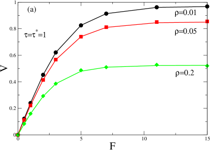
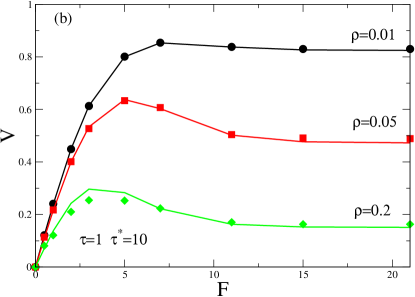
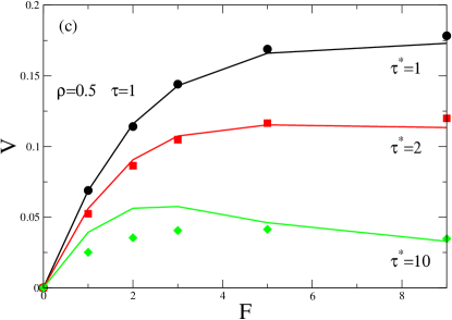
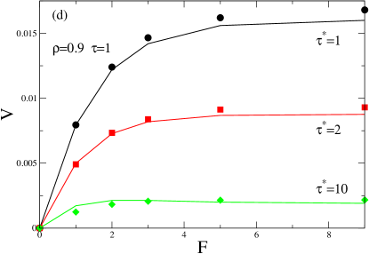
Figure 3: Analytical predictions (continuous lines) and numerical simulations (symbols) for $V(F)$ in the strip-like geometry with $L=3$, and jump probabilities of Choice 1. Parameters are: $\tau=\tau^{*}=1$ (a), $\tau=1,\tau^{*}=10$ (b), $\tau=1$ and $\rho=0.5$ (c), $\tau=1$ and $\rho=0.9$ (d). Notice the nonmonotonic behavior in case (b).

In order to check the validity of the approximation (7) and of the result (12), we have performed Monte Carlo numerical simulations of our model. We have considered a two-dimensional strip-like lattice with $M=L_{1}\times L_{2}$ sites, with $L_{1}=6000$ and $L_{2}=3$, and periodic boundary conditions in both directions. The initial configuration is random with density $\rho=N/M$, $N$ being the number of particles on the lattice. In Fig. 3, we report the analytic results (continuous lines) obtained from the solution of the system for the coefficients $A_{\nu}$, and the numerical data (symbols) from Monte Carlo simulations for the force-velocity relation, for different values of density and time scales, in the case of Choice 1. A very good agreement is observed in a wide range of parameters. As expected, at finite densities, the decoupling approximation turns out to be less accurate at large values of $\tau^{*}$. We also notice that in the case of high density $\rho=0.9$, we found that the relaxation times of the system become very long and an accurate numerical estimation of the stationary velocity requires long simulations.

IV Negative differential mobility and role of microscopic dynamical rules

As shown in Fig. 3(b), in the case with $\tau=1$ and $\tau^{*}=10$, the stationary velocity of the TP shows NDM, namely a nonmonotonic behavior with the applied force. In the framework of lattice gases LF13 ; BM14 ; BIOSV14 this behavior occurs due to the formation of long-lived traps caused by the crowding of bath particles in front of the tracer. Since the TP cannot push the obstacles away, when the dynamics of bath particles is slow enough, namely for large $\tau^{*}$, an increasing of the external force produces a longer escape time from the traps, resulting in a reduction of the average drift.

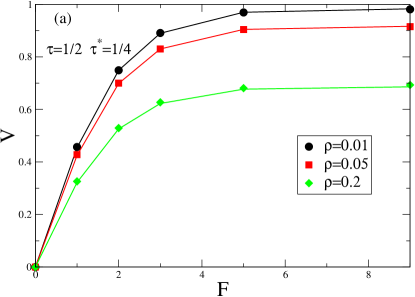
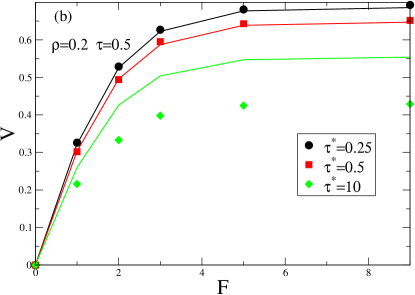
Figure 4: Analytical predictions (continuous lines) and numerical simulations (symbols) for $V(F)$ in the strip-like geometry with $L=3$, and with jump probabilities of Choice 2, with $\tau=0.5$ and $\tau^{*}=0.25$, for different values of $\rho$ (a), and $\rho=0.2,\tau=0.5$ and different values of $\tau^{*}$ (b).

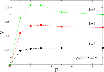
Figure 5: Numerical simulations for $V(F)$ in the strip-like geometry with $L=3,4,5$ for the model with transition probabilities of Choice 2, with $\tau=0.5$, $\tau^{*}=250$ and $\rho=0.2$ (dashed lines are a guide to the eye). The nonmonotonic behavior can be observed for $L\geq 4$.

The complete phase chart identifying the region in the parameter space $\{\rho,\tau^{*}/\tau\}$ where the phenomenon is expected to occur has been obtained in BIOSV14 for infinite lattices, in the case of Choice 1. Here we focus on the case of confined geometry and on the role of the microscopic dynamical rules. Indeed, these can deeply modify the region in the parameter space where NDM occurs. In order to elucidate this important point, we also apply our theory to the model where the transition rates are independent of the field in the transverse direction. These rates have been used for instance in the numerical simulations described in BM14 , and, in our formalism, correspond to Choice 2. As mentioned above, in our theory the specific form of transition rates only enters the last step of the computation, where the numerical solution of the nonlinear system for the coefficients $A_{\nu}$, Eq. (LABEL:system), is carried out. Therefore, the application to the model with jump probabilities of Choice 2 is straightforward. In Fig. 4 we compare the prediction of our analytic solutions for this model with the results of numerical simulations for some cases, finding a very good agreement for not too large values of $\tau^{*}$.

As shown numerically in BM14 for unconfined geometries, and as also discussed in BIOSV14 , a nonmonotonic behavior of $V(F)$ for Choice 2 is observed for large values of $\tau^{*}/\tau$ footnote3 . In this regime, the decoupling approximation is expected not to be accurate, because the bath particles are very slow and their motion is strongly correlated. Moreover, it is important to notice that, in the case of Choice 2, in two dimensions, trapping arises as a three-particle effect: indeed, in order to form a trap one needs an obstacle in front of the TP and two others on the adjacent sites, in the orthogonal directions (see also the discussion in BSV15 ). Therefore, in the case of confined geometries, a NDM cannot be observed for a stripe with $L=3$, because in this case the trapping time becomes independent of the applied force (the TP has no chance to escape the trap and has to wait for the obstacles to step away, for any value of the external field). However, interestingly, as shown in Fig. 5 via numerical simulations, the phenomenon occurs for $L\geq 4$, and sufficiently large values of $\tau^{*}/\tau$.

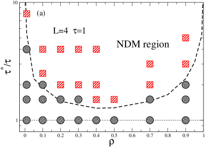
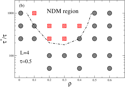
Figure 6: (a) Phase chart for the NDM region in the plane $\tau^{*}/\tau$ vs $\rho$ in the case of Choice 1, for a strip-like geometry with $L=4$. The bold dashed line represents the line separating the region where NDM occurs, according to the analytical solution based on the decoupling approximation. (b) Phase chart for the model with jump probabilities of Choice 2. The dot-dashed line is a guide to the eye. The red squares (black circles) represent numerical simulations where the NDM effect is (is not) observed.

In order to obtain a complete picture and to explicitly show the qualitative difference of behavior that the choice of transition rates can produce, we have reconstructed the phase charts where the effect of NDM is expected to occur, in the parameter space $\tau^{*}/\tau$ vs $\rho$, for both Choice 1 and Choice 2, focusing on the case of a strip-like geometry with $L=4$, see Fig. 6. In the case of Choice 1, the decoupling approximation turns out to be very accurate in predicting quantitatively the range of parameters for which the NDM occurs, as represented by the bold dashed line in Fig. 6(a). Moreover, in this case, from the linearized solution, Eqs. (LABEL:v_lin) and (LABEL:sys_lin), an exact criterion for NDM can be obtained in the low density limit. Following the procedure described in BIOSV14 , we find that the line separating the region of NDM from that where the effect does not occur in the plane $\tau^{*}/\tau$ vs $\rho$ obeys the same scaling observed in unconfined geometries, namely $\tau^{*}/\tau\sim 1/\sqrt{4\rho}$, for $\tau^{*}/\tau\to\infty$.

In the case with jump probabilities of Choice 2, it turns out that the analytical approach based on the decoupling approximation predicts NDM in a region of the parameter space where it is actually not observed via numerical simulations. This is due to the larger values of $\tau^{*}/\tau$ required for NDM to occur, so that the decoupling approximation is not accurate, and cannot account quantitatively for NDM. The phase chart for this choice of transition rates obtained via numerical simulations is reported in Fig. 6(b) footnote3bis .

Our results bring to the fore the important and general issue concerning the choice of microscopic dynamical rules for nonequilibrium systems. Indeed, in the nonlinear regime, different transition rates, all satisfying the LDB, can produce different behaviors. The correct choice should be dictated by physical considerations, and depends on the real system under study. On the one hand, Choice 1 includes the case of totally directed motion, that can be useful to model the dynamics of molecular motors, or the case of a force which reduces the excursions of the TP in the transverse directions. On the other hand, Eq. (2) can be more realistic for systems where the motion in the different directions is totally decoupled, as, e.g., for Brownian dynamics in two or three dimensions, with a force applied along a given direction.

To sum up: i) the general formalism proposed holds for any form of jump probabilities, in particular for Choice 1 and Choice 2; ii) NDM is observed in both cases in confined geometries, as soon as $\L\geq 4$ for the case of Choice 2; iii) our analytical results based on the decoupling approximation account quantitatively for the phenomenon in the case of Choice 1; iv) the theory predicts only qualitatively NDM in the case of Choice 2.

V Density profiles around the tracer particle

In this Section we focus on the study of the bath particle density distribution around the tracer. This quantity plays a central role in the characterization of the micro-structural changes induced by the probe in the host medium and these heterogeneous deformations are responsible for the effective drag coefficient acting on the tracer.

V.1 Two-dimensional infinite lattice

The density profile at large distance from the probe for the case of a two-dimensional infinite lattice has been described in BCCMO01 . It is found that the decay of the density profile in front and past the TP shows two different behaviors. In particular, the asymptotic large distance behavior for the density profile in front of the tracer is exponential:

$$h_{n,0}\sim K_{+}\frac{e^{-n/\lambda_{+}}}{n^{1/2}},$$ (16)

where $K_{+}$ is a coefficient depending on $\{A_{\nu}\}$ and $\rho$ (the explicit expression is given in BCCMO01 ), and $\lambda_{+}$ is the decay length, see BCCMO01 . Remarkably, the wake past the tracer particle shows a different, algebraic, behavior

$$h_{-n,0}=-\frac{K_{-}}{n^{3/2}}\left(1+\frac{3}{8n}+\mathcal{O}(1/n^{2})\right),$$ (17)

where the coefficient $K_{-}$ depends on $\{A_{\nu}\}$ and $\rho$, and is reported in BCCMO01 . Note that this algebraic decay has also been shown to occur in soft dense colloids DBJ14 .

V.2 Strip-like geometry

In confined geometries the theoretical prediction of the density profile around the TP can be obtained numerically for arbitrary values of the distance $n$ from Eq. (LABEL:system). An explicit analytical form can be derived for large distances from the TP. In Appendix B we present the detailed computation of the asymptotic density profile around the tracer focusing on the case of a strip-like geometry, namely for a two-dimensional lattice, infinite in the field direction and of size $L$ in the transverse direction, with periodic boundary conditions. The main result of our computation is that, at variance with the unconfined case, the density profile displays an exponential decay both in front and past the tracer.

V.2.1 Density profiles in the wake of the tracer

As shown in Appendix B, the density profiles in the wake of the tracer in the limit $n\to-\infty$ is

$$h_{n,0}\underset{n\to-\infty}{\sim}\mathcal{H}^{-}\mathrm{e}^{n/\ell^{-}},$$ (18)

with

$$\mathcal{H}^{-} = \frac{2}{L\widetilde{A}_{1}[U_{1}(1)-U_{2}(1)]}\Big{\{}\widetilde{A}_{1}h_{1}[U_{1}(1)^{-1}-1]$$ (19)

$$+ \widetilde{A}_{-1}h_{-1}[U_{1}(1)-1]+2\widetilde{A}_{2}h_{2}\left(\cos\frac{2\pi}{L}-1\right)$$

$$- \rho(\widetilde{A}_{1}-\widetilde{A}_{-1})[U_{1}(1)-U_{1}(1)^{-1}]\Big{\}},$$

$$\ell^{-} = \frac{1}{\ln[U_{1}(1)]},$$ (20)

where $\widetilde{A}_{\mu}$ and the function $U_{1}$ are defined in Appendix B. One can check that $U_{1}(1)>1$ so that $\ell^{-}>0$. Our computation shows that, in contrast with what was found for infinite lattices, the density profile past the tracer in confined geometries presents an exponential decay. This is a surprising result, because one could have expected a behavior intermediate between that of an infinite lattice and that of a one-dimensional single-file for which there is no stationary density profile BOMR96 . On the contrary, what we find here is analogous to the behavior observed in the study of biased diffusion in a one-dimensional adsorbed monolayer BCLMO99 . The exponential decay is related to the fast homogenization in the transverse direction due to confinement. Let us also notice that from the solution of the system (LABEL:system) and the expression (20), we obtain that the decay length $\ell^{-}$ diverges with the stripe width $L$.

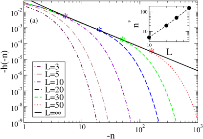
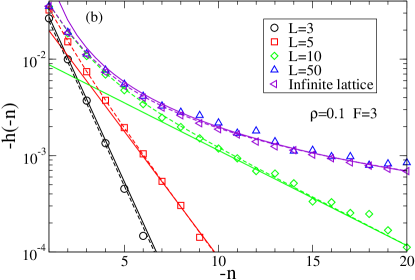
Figure 7: (a) Analytical predictions from Eq. (LABEL:system) for the (rescaled) density profile past the tracer $h(n)$, for different values of the stripe length $L=3,5,10,20,30,50$, with parameters $\tau=\tau^{*}=1$, density $\rho=0.1$, and $F=3$. The black continuous line represents the asymptotic prediction in the case of an infinite lattice, Eq. (17). The stars represent the estimated values of the crossover length $n^{*}$. Inset: characteristic crossover length $n^{*}$ as a function of $L$. (b) Analytical predictions from Eq. (LABEL:system) (dashed lines), asymptotic analytic predictions, Eqs. (18-20) and (17) (continuous lines), and numerical simulations (symbols) of $h(n)$, for different values of the strip length $L=3,5,10,50$, with $\tau=\tau^{*}=1$.

In Fig. 7(a) we show the (rescaled) density profile $h(n)$ past the tracer obtained from the complete analytic solution of Eq. (LABEL:system), for different stripe lengths $L$. Interestingly, we observe a change of behavior from an initial algebraic relaxation, to a final exponential decay. This allows us to identify a characteristic length scale $n^{*}$, governing the crossover between the two regimes. This length diverges with increasing $L$, as expected from the known results for infinite lattices. In particular, it is found that the behavior of the crossover length as a function of $L$ follows a power law, $n^{*}(L)\sim L^{\gamma}$, with $\gamma\simeq 2$, see inset of Fig. 7(a). This can be understood by considering that the diffusional time $t^{*}$ for homogenization in the transverse direction is $t^{*}\sim L^{2}/D$, where $D$ is a diffusion coefficient. Since the TP travels at average velocity $V$, the characteristic crossover length can be then estimated as $n^{*}\sim Vt^{*}\sim VL^{2}/D$.

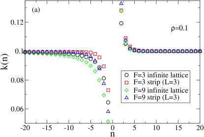
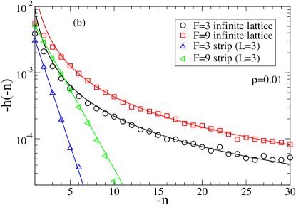
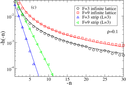
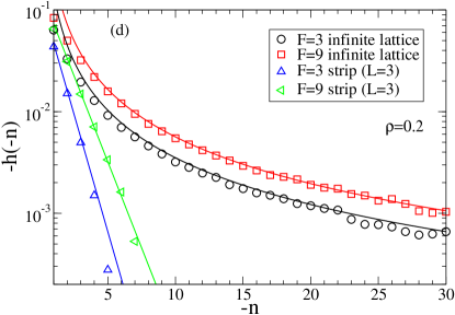
Figure 8: (a) Numerical simulations results for the stationary density profile $k(n)$ (defined in Eq. (5)) in the infinite lattice and in the strip-like geometry, with $\tau=\tau^{*}=1$, $\rho=0.1$ and different values of the force $F$. (b)-(d) Asymptotic analytical predictions, Eqs. (18-20) and (17) (continuous lines) and numerical simulations (symbols) for the (rescaled) density profile past the tracer $h(n)$ in the infinite lattice and in the strip-like geometry, with $\tau=\tau^{*}=1$ and different values of $\rho$.

V.2.2 Density profiles in front of the tracer

In Appendix B we show that, considering for simplicity the special case where $L$ is even, the density profiles in front of the tracer at large distances are given by

$$h_{n,0}\underset{n\to\infty}{\sim}\mathcal{H}^{+}\mathrm{e}^{-n/\ell^{+}},$$ (21)

with

$$\mathcal{H}^{+} = \frac{2}{L\widetilde{A}_{1}[U_{1}(L/2)-U_{2}(L/2)]}\Big{\{}\widetilde{A}_{1}h_{1}[U_{2}(L/2)^{-1}-1]$$ (22)

$$+ \widetilde{A}_{-1}h_{-1}[U_{2}(L/2)-1]+2\widetilde{A}_{2}h_{2}\left(\cos\frac{2\pi}{L}-1\right)$$

$$-\rho(\widetilde{A}_{1}-\widetilde{A}_{-1})[U_{2}(L/2)-U_{2}(L/2)^{-1}]\Big{\}},$$

$$\ell^{+} = -\frac{1}{\ln[U_{2}(L/2)]},$$ (23)

where the function $U_{2}$ is defined in Appendix B. One can check that $U_{2}(L/2)<1$ so that $\ell^{+}>0$. The characteristic length $\ell^{+}$ rapidly converges to the value of the unconfined geometries with the stripe size $L$.

V.3 Comparison with numerical simulations

In Fig. 7(b), we compare results of numerical simulations and analytical predictions for different values of the stripe length $L$, at fixed density $\rho=0.1$ and fixed characteristic times $\tau=\tau^{*}=1$, finding a very good agreement. The continuous lines represent the asymptotic results, Eqs. (18-20) and (17), while the dashed lines represent the complete solution for $h(n)$, valid for arbitrary $n$, obtained from Eq. (LABEL:system). Notice that for intermediate values of $L$ a crossover between the algebraic and the exponential decay can be observed, as predicted by our analytical solution.

The density profiles around the tracer $k(n)$ measured in numerical simulations for density $\rho=0.1$ and two values of the force $F=3,9$, are reported in Fig. 8(a), in the case of Choice 1 footnote4 . In Figs. 8(b)-(d) we report the (rescaled) bath particle density profiles $h(n)$ in the wake past the TP in both infinite and confined geometries, for different values of $\rho$ and $F$. The analytical asymptotic predictions for infinite lattices, Eq. (17), and confined geometries, Eqs. (18-20), represented by continuous lines, are in very good agreement with the numerical simulations (symbols). In simulations the infinite lattice is realized with $L_{1}=L_{2}=200$, with periodic boundary conditions, and the strip-like geometry with $L_{1}=6000$ and $L_{2}=3$.

VI Conclusion

We have studied analytically the dynamics of a driven tracer, traveling in a sea of unbiased hard-core particles on a lattice, in the relevant case of confined geometries. Our general theory unifies and extends previous results, can be applied to any choice of jump probabilities and for arbitrary particle density, and allows us to obtain the force-velocity relation of the TP and the density profiles around it. The central point of our approach is based on a decoupling approximation for the site occupation variable correlation function.

Our treatment allowed us to address some important issues in the study of the nonlinear response of a many-body interacting system. First, regarding the force-velocity relation of the TP, we have shown that our analytical theory is in very good agreement with Monte Carlo numerical simulations, in a wide range of model parameters. In particular, we have found that, in confined geometries also, $V(F)$ in the nonlinear regime can display a nonmonotonic behavior, namely a negative differential mobility. This phenomenon is due to the trapping effect induced by the bath particle on the tracer when the applied field is strong. If the mean characteristic time of the bath particles is sufficiently large, the traps can be long-lived and this produces a decrease of the stationary drift as a function of the force. The microscopic mechanism inducing the trapping effect can depend on the specific dynamical rules of the model BIOSV14 ; BSV15 . We have discussed in detail the different behaviors arising from two particular definitions of jump probabilities BM14 ; BIOSV14 , identifying the region in the parameter space where NDM can take place. In the case of transition rates corresponding to the case of Choice 1, our theory successfully predicts the phase chart where NDM is expected to occur. In the case of Choice 2, the decoupling approximation qualitatively predicts NDM, but cannot account for the phenomenon in the right region of the parameter space, because NDM takes place only when the bath particles are very slow, and their motion is strongly correlated.

The second important issue we have addressed regards the study of the density profiles around the TP, and the local deformations induced in the surrounding medium. We have found that, quite surprisingly, the density profile past the tracer strongly depends on the geometry of the system. In the case of an infinite lattice with $d>1$, it is known that the decay is algebraic BCCMO01 , while for strip-like geometries our theory predicts an exponential decay. Our analytical results also allow us to describe the passage from the algebraic decay to the exponential relaxation, as a function of the strip size. Remarkably, we found that this change of behavior is governed by a characteristic length arising in the density profile, that scales with the stripe size as $\sim L^{2}$. For short distances with respect to this length scale an algebraic decay is expected, while at larger distances the exponential relaxation takes place. Since this length scale diverges with the stripe size, for infinite lattices only the algebraic decay survives.

Our findings show how the structure and shape of the density profile are significantly affected by the lattice geometry. This can have important implications for many known phenomena related to the perturbation profile induced by a tracer in a host medium, such as drifting steady-state structures LZ97 , bath-mediated interactions of driven particles MO10 ; KL15 , and “negative” mass transport LK10 . Moreover, it would be interesting to check if a change of behavior similar to that observed for discrete lattices between infinite and confined geometries is also found in off-lattice systems, such as colloidal suspensions or granular media.

Appendix A Stationary velocity

In this Appendix we present the details on the computations of the TP stationary velocity in a confined geometry in dimension $d$. The functions $h(\boldsymbol{\lambda};t)$, defined by

$$h(\boldsymbol{\lambda};t)\equiv k(\boldsymbol{\lambda};t)-\rho,$$ (24)

with the convention $h({\bf 0};t)=0$, satisfy the following equations of motion

$$2d\tau^{*}\partial_{t}h(\boldsymbol{\lambda};t) = \widetilde{L}h(\boldsymbol{\lambda};t)\quad\textrm{for}\quad{\boldsymbol{\lambda}}\notin\{{\bf 0},\pm\boldsymbol{e}_{1},\ldots,\pm\boldsymbol{e}_{d}\}$$

$$2d\tau^{*}\partial_{t}h(\boldsymbol{\lambda};t) = \widetilde{L}h(\boldsymbol{\lambda};t)+\rho(A_{\nu}-A_{-\nu})$$ (26)

$$\quad\textrm{for}\quad{\boldsymbol{\lambda}}\in\{{\bf 0},\pm\boldsymbol{e}_{1},\ldots,\pm\boldsymbol{e}_{d}\},$$

with $\widetilde{L}\equiv\sum_{\mu}A_{\mu}\nabla_{\mu}$ and $A_{\mu}=1+(2d\tau^{*}/\tau)p_{\mu}[1-\rho-h(\boldsymbol{e}_{\mu})]$.

We introduce the auxiliary variable $\boldsymbol{\xi}=(\xi_{1},\dots,\xi_{d})$ and the generating function

$$H(\boldsymbol{\xi};t)=\sum_{n_{1}=-\infty}^{\infty}\sum_{n_{2},\cdots,n_{d}=0}^{L-1}h_{n_{1},\cdots,n_{d}}(t)\prod_{j=1}^{d}\xi_{j}^{n_{j}},$$ (27)

where the shorthand notation $h(n_{1}\boldsymbol{e}_{1}+\dots+n_{d}\boldsymbol{e}_{d};t)=h_{n_{1},\dots,n_{d}}(t)$ has been used. If $(n_{1},\dots,n_{d})=\boldsymbol{e}_{\nu}$ then we denote $h_{\boldsymbol{e}_{\nu}}=h_{\nu}$. From Eqs. (A) and (26) we can show that $H(\boldsymbol{\xi};t)$ is the solution of the following partial differential equation

$$2d\tau^{*}\partial_{t}H(\boldsymbol{\xi};t) = \left[\frac{A_{1}}{\xi_{1}}+A_{-1}\xi_{1}+A_{2}\sum_{j=2}^{d}\left(\frac{1}{\xi_{j}}+\xi_{j}\right)-\alpha\right]$$ (28)

$$\times H(\boldsymbol{\xi};t)+K(\boldsymbol{\xi};t),$$

with $\alpha=A_{1}+A_{-1}+2(d-1)A_{2}$ and

$$K(\boldsymbol{\xi};t) = A_{1}(\xi_{1}-1)h_{1}(t)+A_{-1}\left(\frac{1}{\xi_{1}}-1\right)h_{-1}(t)$$ (29)

$$+ A_{2}\sum_{j=2}^{d}\left[(\xi_{j}-1)h_{j}(t)+\left(\frac{1}{\xi_{j}}-1\right)h_{-j}(t)\right]$$

$$+ \rho(A_{1}-A_{-1})\left(\xi_{1}-\frac{1}{\xi_{1}}\right).$$

The stationary solution of Eq. (28) is

$$H(\boldsymbol{\xi})=\frac{K(\boldsymbol{\xi})}{\alpha}\frac{1}{1-\left[\frac{A_{1}}{\alpha}\frac{1}{\xi_{1}}+\frac{A_{-1}}{\alpha}\xi_{1}+\frac{A_{2}}{\alpha}\sum_{j=2}^{d}\left(\frac{1}{\xi_{j}}+\xi_{j}\right)\right]}.$$ (30)

We then rewrite the auxiliary variables as $\xi_{1}=\mathrm{e}^{iq}$ and $\xi_{j}=\mathrm{e}^{2i\pi k_{j}/L}$ (for $j\neq 1$), and introduce the function

$$F_{\boldsymbol{n}}=\frac{1}{L^{d-1}}\sum_{k_{2},\dots,k_{d}=0}^{L-1}\frac{1}{2\pi}\int_{-\pi}^{\pi}dq\frac{e^{-in_{1}q}\prod_{j=2}^{d}e^{-2i\pi n_{j}k_{j}/L}}{1-\lambda(q,k_{2},\dots,k_{d})},$$ (31)

with

$$\lambda(q,k_{2},\dots,k_{d})=\frac{A_{1}}{\alpha}\mathrm{e}^{-iq}+\frac{A_{-1}}{\alpha}\mathrm{e}^{iq}+\frac{2A_{2}}{\alpha}\sum_{j=2}^{d}\cos\left(\frac{2\pi k_{j}}{L}\right),$$ (32)

so that $H(\boldsymbol{\xi})$ can be cast in the form

$$H(q,k_{2},\dots,k_{d})=\frac{K(q,k_{2},\dots,k_{d})}{\alpha}\frac{1}{1-\lambda(q,k_{2},\dots,k_{d})}.$$ (33)

Using the definition of $F_{\boldsymbol{n}}$, we get

$$\frac{1}{1-\lambda(q,k_{2},\dots,k_{d})} = \sum_{n_{1}=-\infty}^{\infty}\sum_{n_{2},\dots,n_{d}=0}^{L-1}e^{in_{1}q}$$

$$\times \prod_{j=2}^{d}e^{2i\pi n_{j}k_{j}/L}F_{n_{1},\dots,n_{d}},$$

and

$$H(q,k_{2},\dots,k_{d}) = \frac{1}{\alpha}\sum_{n_{1}=-\infty}^{\infty}\sum_{n_{2},\dots,n_{d}=0}^{L-1}K(q,k_{2},\dots,k_{d})$$ (35)

$$\times F_{n_{1},\dots,n_{d}}e^{in_{1}q}\prod_{j=2}^{d}e^{2i\pi n_{j}k_{j}/L}.$$

Finally, the definition of $K$ in Eq. (29) allows us to show that $h_{n_{1},\dots,n_{d}}$ is given by the system of $2d$ equations (LABEL:system).

Appendix B Density profiles

In this Appendix we present details on the computation of the density profiles around the TP in the case of a strip-like geometry. For simplicity, we introduce $\widetilde{A}_{\nu}=A_{\nu}/\alpha$ (and then $\sum_{\nu}\widetilde{A}_{\nu}=1$). Note that Eq. (LABEL:system) is not closed with respect to the density profiles $h_{\boldsymbol{n}}$. A closed form can be obtained as follows: evaluating Eq. (LABEL:system) for $\boldsymbol{n}=\boldsymbol{e}_{1},\boldsymbol{e}_{-1},\boldsymbol{e}_{2}$, one obtains a closed set of equations satisfied by $h_{1}$, $h_{-1}$ and $h_{2}$. These boundary values of $h_{\boldsymbol{n}}$ can be obtained, and $h_{\boldsymbol{n}}$ for arbitrary $\boldsymbol{n}$ can be computed using Eq. (LABEL:system).

In order to obtain an explicit expression for the density profiles, in what follows, we study the asymptotic behavior of $h_{n,0}$ in the limits $n\to\pm\infty$. To this aim, we consider the behavior of the gradients $\nabla_{\nu}F_{n,0}$ in the limits $n\to\pm\infty$. We will use the following expression of $F_{\boldsymbol{n}}$, that can be obtained with the change of variable $u=\mathrm{e}^{\mathrm{i}q}$ and by computing the integral over $u$ with the residue theorem:

$$F_{\boldsymbol{n}} = \frac{1}{L}\sum_{k}^{L-1}\frac{1}{2\pi}\int_{-\pi}^{\pi}\mathrm{d}q\frac{\mathrm{e}^{-\mathrm{i}n_{1}q}\mathrm{e}^{-2\mathrm{i}\pi n_{2}k/L}}{1-\lambda(q,k)}$$ (36)

$$= \frac{1}{L}\sum_{k=0}^{L-1}\mathrm{e}^{-\frac{2\mathrm{i}\pi kn_{2}}{L}}f(n_{1},k),$$ (37)

with

$$f(n_{1},k)=\begin{dcases}\frac{1}{\widetilde{A}_{1}}\frac{{U_{2}(k)}^{n_{1}}}{U_{1}(k)-U_{2}(k)}&\text{if $n_{1}\geq 0$ }\\ \frac{1}{\widetilde{A}_{1}}\frac{{U_{1}(k)}^{n_{1}}}{U_{1}(k)-U_{2}(k)}&\text{if $n_{1}<0$ },\end{dcases}$$ (38)

and

$$U_{\begin{subarray}{c}1\\ 2\end{subarray}}(k) = \frac{1}{2\widetilde{A}_{1}}\left(1-2\widetilde{A}_{2}\cos\frac{2\pi k}{L}\right)$$ (39)

$$\pm \frac{1}{2}\sqrt{\frac{1}{{\widetilde{A}_{1}}^{2}}\left(1-2{\widetilde{A}_{2}}\cos\frac{2\pi k}{L}\right)^{2}-4\frac{\widetilde{A}_{-1}}{\widetilde{A}_{1}}}.$$

We first study the behavior of the gradients $\nabla_{\nu}F_{n,0}$ behind the tracer ($n<0$).

B.0.1 Density profiles in the wake of the tracer

We assume that $n<0$ and use the expression of $F_{\boldsymbol{n}}$ from Eqs. (37), (38) and (39):

$$\nabla_{1}F_{n,0} = F_{n+1,0}-F_{n,0}$$ (40)

$$= \frac{1}{L}\sum_{k=0}^{L-1}\left[f(n+1,k)-f(n,k)\right]$$

$$= \frac{1}{L\widetilde{A}_{1}}\sum_{k=0}^{L-1}\frac{U_{1}(k)-1}{U_{1}(k)-U_{2}(k)}\mathrm{e}^{n\ln[U_{1}(k)]}.$$

The gradient $\nabla_{1}F_{n,0}$ has then an exponential behavior when $n\to-\infty$, dominated by the term of the sum over $k$ for which $U_{1}(k)$ is the smallest. It can be found by considering the function of a continuous variable $\phi_{1}$ defined as: $\phi_{1}(x)=U_{1}(Lx/2\pi)$, for $x\in[0,2\pi]$. $\phi_{1}(x)$ is symmetric with respect to the value $x=\pi$, and reaches a maximum for this value. Consequently,

$$U_{1}(0) = U_{1}(L)$$ (41)

$$U_{1}(1) = U_{1}(L-1)$$

$$\ldots$$

and the smallest value of $U_{1}(k)$ is reached for $k=0$ and $k=L$. We compute $U_{1}(0)$:

$$U_{1}(0)=\frac{1-2\widetilde{A}_{2}}{2\widetilde{A}_{1}}+\frac{1}{2}\sqrt{\frac{(1-2\widetilde{A}_{2})^{2}}{{\widetilde{A}_{1}}^{2}}-4\frac{\widetilde{A}_{-1}}{\widetilde{A}_{1}}},$$ (43)

and using the relation $\widetilde{A}_{1}+\widetilde{A}_{-1}+2\widetilde{A}_{2}=1$, one obtains $U_{1}(0)=1$. The first term of the sum over $k$ in Eq. (40) is then null. We then conclude that the behavior of $\nabla_{1}F_{n,0}$ is dominated by the terms $k=1$ and $k=L-1$:

$$\nabla_{1}F_{n,0}\underset{n\to-\infty}{\sim}\frac{2}{L\widetilde{A}_{1}}\frac{U_{1}(1)-1}{U_{1}(1)-U_{2}(1)}\mathrm{e}^{n\ln[U_{1}(1)]}.$$ (44)

With a similar calculation, one obtains

$$\nabla_{-1}F_{n,0}\underset{n\to-\infty}{\sim}\frac{2}{L\widetilde{A}_{1}}\frac{U_{1}(1)^{-1}-1}{U_{1}(1)-U_{2}(1)}\mathrm{e}^{n\ln[U_{1}(1)]},$$ (45)

and

$$\nabla_{2}F_{n,0} = F_{n,1}-F_{n,0}$$ (46)

$$= \frac{1}{L}\sum_{k=0}^{L-1}\left[\mathrm{e}^{-\frac{2\mathrm{i}\pi k}{L}}f(n,k)-f(n,k)\right]$$

$$= \frac{1}{L\widetilde{A}_{1}}\sum_{k=0}^{L-1}\left(\mathrm{e}^{-\frac{2\mathrm{i}\pi k}{L}}-1\right)\frac{U_{1}(k)^{n}}{U_{1}(k)-U_{2}(k)}.$$

Once again, the sum over $k$ is dominated by the terms $k=1$ and $k=L-1$:

$$\nabla_{2}F_{n,0} \underset{n\to-\infty}{\sim} \frac{1}{L\widetilde{A}_{1}}\frac{\mathrm{e}^{n\ln[U_{1}(1)]}}{U_{1}(1)-U_{2}(1)}$$

$$\times \underbrace{\left(\mathrm{e}^{-\frac{2\mathrm{i}\pi}{L}}-1+\mathrm{e}^{-\frac{2\mathrm{i}\pi(L-1)}{L}}-1\right)}_{=2[\cos(2\pi/L)-1]}$$

$$\underset{n\to-\infty}{\sim} \frac{2}{L\widetilde{A}_{1}}\left(\cos\frac{2\pi}{L}-1\right)\frac{\mathrm{e}^{n\ln[U_{1}(1)]}}{U_{1}(1)-U_{2}(1)}.$$

Using the asymptotic expansions from Eqs. (44), (45) and (LABEL:nab2_behind) in Eq. (LABEL:system), we finally obtain Eqs. (18-20).

B.0.2 Density profiles in front of the tracer

We use the expression of $f(n,k)$ for $n>0$:

$$f(n,k)=\frac{1}{\widetilde{A}_{1}}\frac{{U_{2}(k)}^{n}}{U_{1}(k)-U_{2}(k)}.$$ (51)

Studying the properties of the function $\phi_{2}(x)=U_{2}(Lx/2\pi)$ on the interval $[0,2\pi]$, one can show that, depending on the parity of $L$, the minimum value for $U_{2}(k)$ is reached:

1. once at $k=L/2$ for $L$ even

2. twice at $k=\lfloor L/2\rfloor\pm 1$ for $L$ odd.

For simplicity, we consider the special case where $L$ is even and obtain

$$\nabla_{\pm 1}F_{n,0} \underset{n\to\infty}{\sim} \frac{2}{L\widetilde{A}_{1}}\frac{U_{2}(L/2)^{\pm 1}-1}{U_{1}(L/2)-U_{2}(L/2)}\mathrm{e}^{n\ln[U_{2}(k=L/2)]}$$

$$\nabla_{2}F_{n,0} \underset{n\to\infty}{\sim} \frac{2}{L\widetilde{A}_{1}}\left(\cos\frac{2\pi}{L}-1\right)\frac{\mathrm{e}^{n\ln[U_{2}(L/2)]}}{U_{1}(L/2)-U_{2}(L/2)},$$

and, using Eq. (LABEL:system), we obtain Eqs. (21-23).

References

- (1) T. M. Squires and T. G. Mason, Ann. Rev. Fluid Mech. 42, 413 (2009).
- (2) L. G. Wilson, and W. C. K. Poon, Phys. Chem. Chem. Phys., 13, 10617 (2011).
- (3) D. Weihs, T. G. Mason, and M. A. Teitell, Biophys. J. 91, 4296 (2006).
- (4) A. M. Puertas, and T. Voigtmann, J. Phys.: Condensed Matter 26, 243101 (2014).
- (5) J. Goyon, A. Colin, G. Ovarlez, A. Ajdari, and L. Bocquet, Nature 454, 84 (2008).
- (6) P. Jop, V. Mansard, P. Chaudhuri, L. Bocquet, and A. Colin, Phys. Rev. Lett. 108, 148301 (2012).
- (7) R. Candelier, and O. Dauchot, Phys. Rev. E 81, 011304 (2010).
- (8) T. Wang, M. Grob, A. Zippelius, and M. Sperl, Phys. Rev. E 89, 042209 (2014).
- (9) A. Gnoli, A. Puglisi, A. Sarracino, and A. Vulpiani, PLoS ONE 9, e93720 (2014).
- (10) C. Scalliet, A. Gnoli, A. Puglisi, and A. Vulpiani, Phys. Rev. Lett. 114, 198001 (2015).
- (11) P. S. Burada, P. Hänggi, F. Marchesoni, G. Schmid, and P. Talkner, ChemPhysChem 10, 45 (2009).
- (12) A. Mukhopadhyay, and S. Granick, Curr. Op. Coll. Int. Science 6, 423 (2001).
- (13) R. B. Schoch, J. Han, and P. Renaud, Rev. Mod. Phys. 80, 839 (2008).
- (14) L. Joly, C. Ybert, and L. Bocquet, Phys. Rev. Lett. 84, 046101 (2006).
- (15) O. Bénichou, C. Chevalier, J. Klafter, B. Meyer, and R. Voituriez, Nature Chemistry 2, 472 (2010).
- (16) C. Bechinger, Curr. Op. Coll. Int. Science 7, 204 (2002).
- (17) C. Gutsche, F. Kremer, M. Krüger, M. Rauscher, R. Weeber, and J. Harting, J. Chem. Phys. 129, 084902 (2008).
- (18) P. Tarazona and U. Marini Bettolo Marconi, J. Chem. Phys. 128, 164704 (2008).
- (19) L. Almenar, and M. Rauscher, J. Phys.: Condens. Matter 23, 184115 (2011).
- (20) M. D. Graham, Annu. Rev. Fluid Mech. 43, 273 (2011).
- (21) S. Lang and T. Franosch, Phys. Rev. E 89, 062122 (2014).
- (22) D. Winter, J. Horbach, P. Virnau, and K. Binder, Phys. Rev. Lett. 108, 028303 (2012).
- (23) O. Bénichou, A. Bodrova, D. Chakraborty, P. Illien, A. Law, C. Mejía-Monasterio, G. Oshanin, and R. Voituriez, Phys. Rev. Lett. 111, 260601 (2013).
- (24) T. M. Squires and J. F. Brady, Phys. Fluids 17, 073101 (2005).
- (25) M. Fuchs and M. E. Cates, Phys. Rev. Lett. 89, 248304 (2002).
- (26) T. Wang, and M. Sperl, Preprint arXiv:1504.02277.
- (27) O. Bénichou, A. M. Cazabat, J. De Coninck, M. Moreau, and G. Oshanin, Phys. Rev. Lett. 84, 511 (2000).
- (28) I. C. Carpen and J. F. Brady, J. Rheol. 49, 1483 (2005).
- (29) R. N. Zia and J. F. Brady, J. Fluid. Mech. 658, 188 (2010).
- (30) C. Mejía-Monasterio and G. Oshanin, Soft Matter 7, 993 (2011).
- (31) I. Sriram, A. Meyer, and E. M. Furst, Phys. Fluids 22, 062003 (2010).
- (32) D. Winter and J. Horbach, J. Chem. Phys. 138, 12A512 (2013).
- (33) V. Démery, O. Bénichou, and H. Jacquin, New J. Phys. 16, 053032 (2014).
- (34) J. Dzubiella, H. Löwen, and C. N. Likos, Phys. Rev. Lett. 91, 248301 (2003).
- (35) F. Penna, J. Dzubiella, and P. Tarazona, Phys. Rev. E 68, 061407 (2003).
- (36) M. Rauscher, A. Domínguez, M. Krüger, and F. Penna, J. Chem. Phys. 127, 244906 (2007).
- (37) J. L. Lebowitz and H. Spohn, J. Stat. Phys. 95, 333 (1999).
- (38) K. Mallick, Physica A 418, 17 (2015).
- (39) L. F. Perondi, J. Phys.: Condens. Matter 17, S4165 (2005).
- (40) R. L. Jack, D. Kelsey, J. P. Garrahan, and D. Chandler, Phys. Rev. E 78, 011506 (2008).
- (41) S. Leitmann, and T. Franosch, Phys. Rev. Lett. 111, 190603 (2013).
- (42) P. Baerts, U. Basu, C. Maes, and S. Safaverdi, Phys. Rev. E 88, 052109 (2013).
- (43) U. Basu and C. Maes, J. Phys. A: Math. Theor. 47, 255003 (2014).
- (44) O. Bénichou, P. Illien, G. Oshanin, A. Sarracino, and R. Voituriez, Phys. Rev. Lett. 113, 268002 (2014).
- (45) M. Baiesi, A. L. Stella, and C. Vanderzande, Phys. Rev. E 92, 042121 (2015).
- (46) R. K. P. Zia, E. L. Praestgaard, and O. G. Mouritsen, Am. J. Phys. 70, 384 (2002).
- (47) G. A. Cecchi and M. O. Magnasco, Phys. Rev. Lett. 76, 1968 (1996).
- (48) M. Kostur, L. Machura, P. Hänggi, J. Luczka, and P. Talkner, Physica (Amsterdam) 371A, 20 (2006).
- (49) B. Altaner, A. Wachtel, and J. Vollmer, Phys. Rev. E 92, 042133 (2015).
- (50) M. Sellitto, Phys. Rev. Lett. 101, 048301 (2008).
- (51) E. Lippiello, F. Corberi, and M. Zannetti, Phys. Rev. E 71, 036104 (2005).
- (52) M. Baiesi, C. Maes, and B. Wynants, Phys. Rev. Lett. 103, 010602 (2009).
- (53) E. Lippiello, F. Corberi, A. Sarracino, and M. Zannetti, Phys. Rev. B 77, 212201 (2008); Phys. Rev. E 78, 041120 (2008).
- (54) U. Basu, M. Krüger, A. Lazarescu, and C. Maes, Phys. Chem. Chem. Phys. 17, 6653 (2015).
- (55) U. Basu and C. Maes, J. Phys.: Conf. Ser. 638, 012001 (2015).
- (56) S. F. Burlatsky, G. Oshanin, A. Mogutov, and M. Moreau, Phys. Lett. A 166, 230 (1992).
- (57) O. Bénichou, A. M. Cazabat, A. Lemarchand, M. Moreau, and G. Oshanin, J. Stat. Phys. 97, 351 (1999).
- (58) S. F. Burlatsky, G. Oshanin, M. Moreau, and W. P. Reinhardt, Phys. Rev. E 54, 3165 (1996).
- (59) O. Bénichou, A. M. Cazabat, J. De Coninck, M. Moreau, and G. Oshanin, Phys. Rev. B 63, 235413 (2001).
- (60) O. Bénichou, A. M. Cazabat, M. Moreau, and G. Oshanin, Physica A 272, 56 (1999).
- (61) Remarkably, the latter result for a discrete system appears to be qualitatively very similar to what was found via a dynamic density functional theory PDT03 for a driven colloidal particle moving in polymer solutions, and has been also shown to occur in dense solutions of soft colloids DBJ14 .
- (62) G. Oshanin, O. Bénichou, S. Burlatsky, and M. Moreau, Biased tracer diffusion in hard-core lattice gases: Some notes on the validity of the Einstein relation, in Instabilities and Nonequilibrium Structures IX, edited by O. Descalzi, J. Martinez, and S. Rica (Springer, Dordrecht, 2004).
- (63) Z. Bertalan, Z. Budrikis, C. A. M. La Porta, and S. Zapperi, PLoS ONE 10, e0136945 (2015).
- (64) We expect that reflecting boundary conditions do not change significantly our results.
- (65) Note that the case corresponds to single-files regardless of the dimension .
- (66) B. D. Hughes, Random Walks and Random Environments (Oxford Science, Oxford, 1995).
- (67) In Ref. BM14 the only relevant temporal scale is the inverse of bath particles transition rate , which is related to our parameters by . In the simulations reported in BM14 , for an infinite lattice with density , the phenomenon of negative differential mobility is observed for , corresponding to .
- (68) Notice that for and large values of the times of convergence of numerical simulations are very long and more accurate estimations of the TP velocity would require further analysis.
- (69) Similar behaviors are observed with the choice of Eq. (2).
- (70) K. T. Leung and R. K. P. Zia, Phys. Rev. E 56, 308 (1997).
- (71) O. V. Kliushnychenko and S. P. Lukyanets, Preprint arXiv:1507.06914.
- (72) S. P. Lukyanets and O. V. Kliushnychenko, Phys. Rev. E 82, 051111 (2010).