Sobolev and Max Norm Error Estimates for Gaussian Beam Superpositions

Abstract

This work is concerned with the accuracy of Gaussian beam superpositions, which are asymptotically valid high frequency solutions to linear hyperbolic partial differential equations and the Schrödinger equation. We derive Sobolev and max norms estimates for the difference between an exact solution and the corresponding Gaussian beam approximation, in terms of the short wavelength $\varepsilon$. The estimates are performed for the scalar wave equation and the Schrödinger equation. Our result demonstrates that a Gaussian beam superposition with $k$-th order beams converges to the exact solution as $O(\varepsilon^{k/2-s})$ in order $s$ Sobolev norms. This result is valid in any number of spatial dimensions and it is unaffected by the presence of caustics in the solution. In max norm, we show that away from caustics the convergence rate is $O(\varepsilon^{\lceil k/2\rceil})$ and away from the essential support of the solution, the convergence is spectral in $\varepsilon$. However, in the neighborhood of a caustic point we are only able to show the slower, and dimensional dependent, rate $O(\varepsilon^{(k-n)/2})$ in $n$ spatial dimensions.

1 Introduction

In this paper we consider the accuracy of Gaussian beam approximations for two time-dependent partial differential equations (PDEs) with highly oscillatory solutions: the dispersive Schrödinger equation in the semi-classical regime,

$${}-i\varepsilon u_{t}-\frac{\varepsilon^{2}}{2}\triangle u+V(y)u =0,\qquad(t,y)\in(0,T]\times\mathbb{R}^{n},$$ (1)

$$u(0,y) =B_{0}(y)e^{i\varphi_{0}(y)/\varepsilon}\ ,$$

and the scalar wave equation,

$${}u_{tt}-c(y)^{2}\Delta u =0,\qquad(t,y)\in(0,T]\times\mathbb{R}^{n},$$ (2)

$$u(0,y) =B_{0}(y)e^{i\varphi_{0}(y)/\varepsilon},$$

$$u_{t}(0,y) =\varepsilon^{-1}B_{1}(y)e^{i\varphi_{0}(y)/\varepsilon}.$$

In these equations, $V(y)$ is an external potential, $c(y)$ is the speed of propagation and $\varepsilon\ll 1$ is the short wavelength, or the scaled Planck constant for (1). Since $\varepsilon$ is small, the initial data for both PDEs are highly oscillatory. The amplitude functions $B_{{\ell}}$ and phase $\varphi_{0}$ are real valued functions on $\mathbb{R}^{n}$. We will assume that $c,V,\varphi_{0},B_{\ell}$ are all smooth and that $B_{{\ell}}$ are supported in the compact set $K_{0}\subset\mathbb{R}^{n}$.

Direct numerical simulation of these PDEs is expensive when $\varepsilon$ is small. A large number of grid points is needed to resolve the wave oscillations and the computational cost to maintain constant accuracy grows rapdily with the frequency. As an alternative one can use high frequency asymptotic models for wave propagation, such as geometrical optics [16, 3, 36], which is obtained in the limit when $\varepsilon\to 0$. The solution of the PDE is then written as

$${}u(t,y)=a(t,y,\varepsilon)e^{i\phi(t,y)/\varepsilon},$$ (3)

where $\phi$ is the phase, and $a$ is the amplitude of the solution, which both vary on a much coarser scale than $u$. When $\varepsilon\to 0$ the phase and amplitude are independent of the frequency. Therefore, they can be computed at a computational cost independent of the frequency. However, at caustics where rays concentrate, geometrical optics breaks down and the predicted amplitude becomes unbounded, [28, 19].

Gaussian beams form another high frequency asymptotic model which is closely related to geometrical optics [33, 31, 15, 2, 17, 10, 5]. Unlike geometrical optics, there is no breakdown at caustics. The solution is assumed to be of the same form (3), but a Gaussian beam is a localized solution that concentrates near a single geometrical optics ray $x(t)$ in space-time. We write it as

$$v(t,y)=A(t,y-x(t))e^{i\Phi(t,y-x(t))/\varepsilon}.$$

The concentration comes from the fact that, although the phase function is real-valued along $x(t)$, it has a positive imaginary part away from $x(t)$. Moreover, the imaginary part is quadratic in $y$ so that $\Im\Phi(t,y)\sim|y|^{2}>0$, and therefore $|v(t,y)|\sim e^{-|y-x(t)|^{2}/\varepsilon}$, which means that the beams have essentially a Gaussian shape of width $\sqrt{\varepsilon}$, centered around $x(t)$. Because of this localization one can approximate the amplitude and phase away from $x(t)$ by Taylor expansion; both $\Phi(t,y)$ and $A(t,y)$ are polynomials in $y$. For instance, in first order beams $\Phi(t,y)$ is a second order polynomial, and $A(t,y)$ is a zeroth order (constant) polynomial. The coefficients in the polynomials satisfy ODEs. Higher order Gaussian beams are created by using an asymptotic series for the amplitude and using higher order Taylor expansions for $\Phi(t,y)$ and $A(t,y)$. For higher order beams, a cutoff function is also necessary to avoid spurious growth away from the center ray.

In numerical methods one must consider more general high frequency solutions, which are not necessarily concentrated on a single ray. Superpositions of Gaussian beams are then used. This is natural since the PDEs are linear. If we let $v(t,y,z)$ be a beam starting from the point $y=z$, the Gaussian beam superposition is defined as

$${}u_{GB}(t,y)=\left(\frac{1}{2\pi\varepsilon}\right)^{\frac{n}{2}}\int_{K_{0}}v(t,y,z)dz,$$ (4)

for the set $K_{0}$ where initial data is concentrated. The prefactor normalizes the superposition appropriately, so that $u_{GB}=O(1)$. More details about the construction of Gaussian beam superpositions are given in Section 3.

Numerical methods based on Gaussian beam type superpositions go back to the 1980’s for the wave equation [31, 15, 2, 17, 39] and for the Schrödinger equation [6, 7]. Since then a great many such methods have been developed for various applications [8, 9, 38, 4, 20, 37, 40, 30, 32]. Typically, the ODEs for the Taylor coefficients of the phase and amplitude are solved using numerical ODE methods like Runge–Kutta and the superposition integral (4) is approximated by the trapezoidal rule. There are also Eulerian methods [21, 13, 14] in which PDEs are solved to get the Taylor coefficients on fixed grids. For more discussions of numerical methods using Gaussian beams, see [12, Sections 8–9].

The topic of this paper is the accuracy of Gaussian beam approximations in terms of the wavelength $\varepsilon$. Several such studies have been carried out in recent years. One of the reasons have been to give a rigorous foundation for the beam based numerical methods above. For the time-dependent case error estimates were first derived for the initial data [18, 37], and later for the solution of scalar hyperbolic equations and the Schrödinger equation [23, 24, 26, 41, 22]. For the Helmholtz equation estimates have been given in [29, 25]. The general result is that the error between the exact solution and the Gaussian beam approximation decays as $\varepsilon^{k/2}$ for $k$-th order beams in the appropriate Sobolev norm. However, in the recent paper [41], Zheng showed the improved rate $\varepsilon$ for first order beams ($k=1$) applied to the Schrödinger equation. This rate agrees with the $\varepsilon^{\lceil k/2\rceil}$ rate shown in a simplified setting for the (pointwise) Taylor expansion error away from caustics in [29]. These improved estimates come from exploiting error cancellations between adjacent beams; the higher rate is not present for single beams. There are also estimates for other Gaussian beam like superpositions, in particular for so-called frozen Gaussians [34, 27] and for the acoustic wave equation with superpositions in phase space [1].

In this paper we first derive error estimates in general higher order Sobolev norms for the Schrödinger equation and the scalar wave equation. The result is in Theorem 7 where we obtain a convergence rate of $\varepsilon^{k/2-s}$ for $s$-order Sobolev norms. Since the solution oscillates with period $\varepsilon$, this reduced rate is expected. The proof follows closely the proof in [26] for the case $s=0$. Second, we derive the main result of this paper. It is a max norm estimate given in Theorem 10. All earlier estimates for Gaussian beam approximations that we are aware of, have been in integrated (Sobolev) norms. We believe this is the first max norm estimate. We show that, away from caustics, the error has, uniformly, the faster rate $\varepsilon^{\lceil k/2\rceil}$ shown in [29, 41], which we think is the optimal rate. Close to caustics, our estimate degenerates and we only get the dimensional dependent rate $\varepsilon^{(k-n)/2}$. This rate can likely be improved, at least for certain types of caustics, and a better understanding of this error will be the subject of future research. Finally, away from the essential support of the solution the error, as well as the solution itself, decays at a spectral rate in $\varepsilon$.

The proof of the max norm estimate uses the Sobolev estimates derived in the first part of the paper, together with Sobolev inequalities to first get a rough estimate. It is subsequently refined by analyzing the difference between beam approximations of different orders. We show in Theorem 12 that the difference can be written as a sum of oscillatory integrals with certain properties. The main difficulty lies in making uniform estimates of these integrals; see Theorem 13.

The paper is organized as follows: In Section 2 we introduce notation and state our main assumptions. Section 3 introduces Gaussian beam superpositions for the Schrödinger equation and the wave equation. In Section 4 we show some simple consequences of our assumptions as well as some known results about Gaussian beams. Section 5 and Section 6 are then devoted to proving the error estimates in Sobolev norms and max norm, respectively.

2 Preliminaries

In this section we introduce some notation and describe the assumptions made for the PDEs and their initial data. We also summarize some key well-posedness results.

We write $|x|$ for the Euclidean norm of a vector $x\in\mathbb{R}^{n}$. However, for a multi-index $\alpha=(\alpha_{1},\ldots,\alpha_{n})\in\mathbb{Z}^{n}_{+}$, we use the standard convention that $|\alpha|=\alpha_{1}+\cdots+\alpha_{n}$. We frequently use the simple estimate,

$$|x^{\alpha}|\leq|x|^{|\alpha|},\qquad x\in\mathbb{R}^{n},\quad\alpha\in\mathbb{Z}^{n}_{+}.$$

For a function $f:\mathbb{R}^{n}\mapsto\mathbb{R}$ we let $\nabla f(x)$ denote its gradient, and $D^{2}f(x)$ its Hessian matrix. Partial derivatives of order $\alpha$ is written as $\partial_{x}^{\alpha}f(x)$. For a function $f:\mathbb{R}^{n}\mapsto\mathbb{R}^{n}$ we denote the Jacobian matrix by $Df(x)$.

For function spaces we let $C^{\infty}_{b}(\mathbb{R}^{n})$ be the functions in $C^{\infty}(\mathbb{R}^{n})$ whose derivatives are all bounded. Moreover, $H^{s}(\mathbb{R}^{n})$ denotes the usual Sobolev spaces, with $H^{0}(\mathbb{R}^{n})=L^{2}(\mathbb{R}^{n})$. For these spaces we use the standard norm, and an $\varepsilon$-scaled norm defined as

$${}\|f\|_{H^{s}(\mathbb{R}^{n})}:=\sum_{|\alpha|\leq s}\left\|\partial_{y}^{\alpha}f\right\|_{L^{2}(\mathbb{R}^{n})},\qquad\|f\|_{H_{\varepsilon}^{s}(\mathbb{R}^{n})}:=\sum_{|\alpha|\leq s}\varepsilon^{|\alpha|-s}\left\|\partial_{y}^{\alpha}f\right\|_{L^{2}(\mathbb{R}^{n})}.$$ (5)

We finally define, for continuous $f$,

$${}||f||_{L^{\infty}(K)}:=\sup_{z\in{K}}|f(z)|,\qquad|f|_{{\rm Lip}(K)}:=\sup_{z,z^{\prime}\in K}\frac{|f(z)-f(z^{\prime})|}{|z-z^{\prime}|},$$ (6)

and note that for all $T>0$, compact set $K\subset\mathbb{R}^{n}$ and $f(t,z)\in C^{\infty}([0,T]\times K)$,

$${}\sup_{t\in[0,T]}||f(t,\,\cdot\,)||_{L^{\infty}(K)},\qquad\sup_{t\in[0,T]}|f(t,\,\cdot\,)|_{{\rm Lip}(K)},$$ (7)

are both finite.

We then make the following precise assumptions:

• Smooth and bounded potential; strictly positive, smooth and bounded speed of propagation,

  $$c,V\in C^{\infty}_{b}(\mathbb{R}^{n}),\qquad\inf_{y\in\mathbb{R}^{n}}c(y)>0.$$

• Smooth and compactly supported initial amplitudes,

  $$B_{{\ell}}\in C^{\infty}(\mathbb{R}^{n}),\quad{\rm supp}\,B_{{\ell}}\subset K_{0},\qquad\ell=0,1,$$

  where $K_{0}\subset\mathbb{R}^{n}$ is a compact set.

• Smooth initial phase,

  $$\varphi_{0}\in C^{\infty}(\mathbb{R}^{n}).$$

  For the wave equation we also assume that the initial phase gradient is bounded away from zero,

  $$\inf_{y\in\mathbb{R}^{n}}|\nabla\varphi_{0}(y)|>0.$$

• High frequency,

  $$0<\varepsilon\leq 1.$$

These assumptions imply that there are unique, smooth, solutions of (1) and (2). To be precise, the solutions and their time-derivatives belong to $L^{\infty}([0,T];H^{s}(\mathbb{R}^{n}))$ for all $s\geq 0$ and $T>0$.

The corner stone of our error estimates are the energy estimates for the PDEs. To facilitate the presentation we will use the following notation for the partial differential operators,

$${}P[u]:=u_{tt}-c(y)^{2}\Delta u,\qquad P^{\varepsilon}[u]:=-i\varepsilon u_{t}-\frac{\varepsilon^{2}}{2}\Delta u+V(y)u.$$ (8)

The estimate of the solution of the Schrödinger equation uses the norm in (5). For $s\geq 0$ and $T>0$, there is a constant $C_{s}(T)$ such that whenever $\varepsilon\in(0,1]$,

$${}\sup_{0\leq t\leq T}\|u(t,\,\cdot\,)\|_{H^{s}}\leq C_{s}(T)\left(||u(0,\,\cdot\,)||_{H^{s}_{\varepsilon}(\mathbb{R}^{n})}+\frac{1}{\varepsilon}\sup_{0\leq t\leq T}||P^{\varepsilon}[u](t,\,\cdot\,)||_{H^{s}_{\varepsilon}(\mathbb{R}^{n})}\right).$$ (9)

This estimate is standard for $s=0$. For $s>0$ it follows by induction upon differentiating the Schrödinger equation $s$ times. For the wave equation there is a constant $C_{s}(T)$ for each $s\geq 1$ and $T>0$, such that

$$\sup_{0\leq t\leq T}\left(\|u(t,\,\cdot)\|_{H^{s}(\mathbb{R}^{n})}+\|\partial_{t}u(t,\,\cdot)\|_{H^{s-1}(\mathbb{R}^{n})}\right)$$ (10)

$$\leq C_{s}(T)\left(\|u(0,\,\cdot\,)\|_{H^{s}(\mathbb{R}^{n})}+\|\partial_{t}u(0,\,\cdot\,)\|_{H^{s-1}(\mathbb{R}^{n})}+\sup_{0\leq t\leq T}\|P[u](t,\,\cdot\,)\|_{H^{s-1}(\mathbb{R}^{n})}\right).$$

See e.g. [11, Lemma 23.2.1].

Remark 2.1.

For the Schrödinger equation, we do not need to assume the lower bound on $|\nabla\varphi_{0}|$.

Remark 2.2.

The assumption of $C^{\infty}$ smoothness for all functions is made for simplicity to avoid an overly technical discussion about precise regularity requirements. In this sense, the error estimates given below can be sharpened, since they will be true also for less regular functions.

3 Gaussian Beams

In this section, we briefly describe the Gaussian beam approximation. We restrict the description to the points that are relevant for the accuracy analysis in subsequent sections. For a more detailed account with a general derivation for hyperbolic equations, dispersive wave equations and Helmholtz equation, we refer to [33, 37, 23, 24, 12, 26, 25].

Individual Gaussian beams concentrate around a central ray in space-time. We denote the $k$-th order Gaussian beam and the central ray starting at $z\in K_{0}$ by $v_{k}(t,y,z)$ and $x(t,z)$ respectively. The beam has the following form,

$${}v_{k}(t,y,z)=A_{k}(t,y-x(t,z),z)e^{i\Phi_{k}(t,y-x(t,z),z)/\varepsilon},$$ (11)

where

$${}\Phi_{k}(t,y,z)=\phi_{0}(t,z)+y\cdot p(t,z)+\frac{1}{2}y\cdot M(t,z)y+\sum_{|\beta|=3}^{k+1}\frac{1}{\beta!}\phi_{\beta}(t,z)y^{\beta},$$ (12)

and

$${}A_{k}(t,y,z)=\sum_{j=0}^{\lceil\frac{k}{2}\rceil-1}\varepsilon^{j}\bar{a}_{j,k}(t,y,z),$$ (13)

$${}\bar{a}_{j,k}(t,y,z)=\sum_{|\beta|=0}^{k-2j-1}\frac{1}{\beta!}a_{j,\beta}(t,z)y^{\beta}\ .$$ (14)

Note that none of $\phi_{0}$, $p$, $M$, $\phi_{\beta}$ or $a_{j,\beta}$ depend on $k$.

Single beams are summed together to form the $k$-th order Gaussian beam superposition solution $u_{k}(t,y)$,

$${}u_{k}(t,y)=\left(\frac{1}{2\pi\varepsilon}\right)^{\frac{n}{2}}\int_{K_{0}}v_{k}(t,y,z)\varrho_{\eta}(y-x(t,z))dz,$$ (15)

where the integration in $z$ is over the support of the initial data $K_{0}\subset\mathbb{R}^{n}$. The function $\varrho_{\eta}\in C^{\infty}(\mathbb{R}^{n})$ is a real-valued cutoff function with radius $0<\eta\leq\infty$ satisfying,

$${}\varrho_{\eta}(z)\geq 0\quad\mbox{ and }\quad\varrho_{\eta}(z)=\left\{\begin{array}[]{ll}\begin{array}[]{l}1\mbox{ for }|z|\leq\eta,\\ 0\mbox{ for }|z|\geq 2\eta,\end{array}&\mbox{ for }0<\eta<\infty,\\ \begin{array}[]{l}1,\end{array}&\mbox{ for }\eta=\infty.\end{array}\right.$$ (21)

As shown below in Lemma 2, if $\eta>0$ is sufficiently small, it is ensured that $\Im\Phi_{k}>0$ on the support of $\varrho_{\eta}$ and the Gaussian beam superposition is well-behaved. For first order beams, $k=1$, the cutoff function is not needed and we can take $\eta=\infty$.

Since the wave equation (2) is a second order equation two modes and two Gaussian beam superpositions are needed, one for forward and one for backward propagating waves. We denote the corresponding coefficients by a $+$ and $-$ superscript, respectively, and write

$${}u_{k}(t,y)=\left(\frac{1}{2\pi\varepsilon}\right)^{\frac{n}{2}}\int_{K_{0}}[v^{+}_{k}(t,y,z)+v^{-}_{k}(t,y,z)]\varrho_{\eta}(y-x(t,z))dz,$$ (22)

where $v_{k}^{\pm}$ are built from the central rays $x^{\pm}(t,z)$ and coefficients $\phi_{0}^{\pm}$, $p^{\pm}$, $M^{\pm}$, $\phi^{\pm}_{\beta}$, $a^{\pm}_{j,\beta}$.

3.1 Governing ODEs

The central rays $x(t,z)$ and all the coefficients $\phi_{0}$, $p$, $M$, $\phi_{\beta}$ and $a_{j,\beta}$ satisfy ODEs in $t$. The dependence on $z$ is only via the initial data.

For the Schrödinger equation the leading order ODEs are

$$\partial_{t}x =p,$$ (23a)

$$\partial_{t}p =-\nabla V(x),$$ (23b)

$$\partial_{t}\phi_{0} =\frac{|p|^{2}}{2}-V(x),$$ (23c)

$$\partial_{t}M =-M^{2}-D^{2}V(x),$$ (23d)

$$\partial_{t}a_{0} =-\frac{1}{2}{\rm Tr}(M)a_{0}.$$ (23e)

The ODEs for the higher order coefficients $\phi_{\beta}$ and $a_{j,\beta}$ are more complicated. The phase derivatives $\phi_{\beta}$ can be solved recursively in such a way that all ODEs are linear. They are of the form

$$\partial_{t}\phi_{\beta}=-\frac{1}{2}\sum_{j=1}^{n}\mathop{\sum_{|\gamma|=1}}_{\gamma\leq\beta}^{|\beta|-1}\frac{\beta!}{(\beta-\gamma)!\gamma!}\phi_{\beta-\gamma+e_{j}}\phi_{\gamma+e_{j}}-\partial_{y}^{\beta}V,\qquad|\beta|\geq 3\ .$$

The amplitude terms $a_{j,\beta}$ satisfy a big linear system of ODEs of the form

$${}\partial_{t}{\mathbf{a}}(t,z)={\mathbf{A}}(t,z){\mathbf{a}}(t,z),$$ (24)

where ${\mathbf{a}}$ is a vector containing all coefficients $\{a_{j,\beta}\}$ and ${\mathbf{A}}$ is a matrix determined from the phase terms $\{\phi_{\beta}\}$. Moreover, ${\mathbf{A}}$ is lower block triangular if the elements of ${\mathbf{a}}$ is ordered with increasing $|\beta|$; $\partial_{t}a_{j,\beta}$ only depends on $a_{j,\beta^{\prime}}$ with $|\beta^{\prime}|\leq|\beta|$. We refer to [33, 37] for more detailed discussions.

The leading order ODEs for the two modes of the wave equation are

$$\partial_{t}x^{\pm} =\pm c(x^{\pm})\frac{p^{\pm}}{|p^{\pm}|},$$ (25a)

$$\partial_{t}p^{\pm} =\mp\nabla c(x^{\pm})|p^{\pm}|,$$ (25b)

$$\partial_{t}\phi^{\pm}_{0} =0,$$ (25c)

$$\partial_{t}M^{\pm} =\mp(E+B^{T}M^{\pm}+M^{\pm}B+M^{\pm}CM^{\pm}),$$ (25d)

$$\partial_{t}a^{\pm}_{0} =\pm\frac{1}{2|p^{\pm}|}\left(p^{\pm}\cdot\nabla c(x^{\pm})+\frac{c(x^{\pm})\>p^{\pm}\cdot Mp^{\pm}}{|p^{\pm}|^{2}}-c(x^{\pm})\>\text{Tr}(M^{\pm})\right)a^{\pm}_{0},$$ (25e)

with

$$E=|p^{\pm}|D^{2}c(x^{\pm}),\qquad B=\frac{p^{\pm}\otimes\nabla c(x^{\pm})}{|p^{\pm}|},\qquad C=\frac{c(x^{\pm})}{|p^{\pm}|}{\rm Id}_{n\times n}-\frac{c(x^{\pm})}{|p^{\pm}|^{3}}p^{\pm}\otimes p^{\pm}.$$

The higher order phase terms $\{\phi^{\pm}_{\beta}\}$ again satisfy linear ODEs, if solved in the right order, and the higher order amplitude terms $\{a^{\pm}_{j,\beta}\}$ satisfy a linear ODE system of the type (24).

Remark 3.1.

The leading order ODEs for both equations, and for general hyperbolic equations, actually have a Hamiltonian structure,

$$\partial_{t}x =\nabla_{p}H(x,p),$$ (26a)

$$\partial_{t}p =-\nabla_{x}H(x,p),$$ (26b)

$$\partial_{t}\phi_{0} =-H(x,p)+p\cdot\nabla_{p}H(x,p),$$ (26c)

where $H=|p|^{2}/2+V(x)$ for the Schrödinger equation and $H=\pm c(x)|p|$ for the two modes of the wave equation.

3.2 Initial Data

Each Gaussian beam $v_{k}(t,y,z)$ requires initial values for the central ray and all of the amplitude and phase Taylor coefficients. The appropriate choice of these initial values will make $u_{k}(0,y)$ asymptotically converge to the initial conditions in (1) and (2). As shown in [26], initial data for the central ray and phase coefficients should be chosen as follows, for the Schrödinger as well as the two modes of the wave equation.

$$x(0,z) =z,$$ (27a)

$$p(0,z) =\nabla\varphi_{0}(z),$$ (27b)

$$\phi_{0}(0,z) =\varphi_{0}(z),$$ (27c)

$$M(0,z) =D^{2}\varphi_{0}(z)+i\ {\rm Id}_{n\times n},$$ (27d)

$$\phi_{\beta}(0,z) =\partial_{y}^{\beta}\varphi_{0}(z),\qquad|\beta|=3,\ldots,k+1\ .$$ (27e)

For the Schrödinger equation, initial values for the amplitude coefficients should be given as

$${}a_{j,\beta}(0,z)=\begin{cases}\partial_{y}^{\beta}B_{0}(z),&j=0,\\ 0,&j>0.\end{cases}$$ (28)

The construction is more complicated for the wave equation. Let

$$\bar{A}^{\pm}_{0}(y,z) =\frac{1}{2}\left(B_{0}(y)+\frac{B_{1}(y)}{id_{t}\Phi^{\pm}_{k}(0,y-z,z)}\right),$$

$$\bar{A}^{\pm}_{j+1}(y,z) =-\frac{1}{2}\frac{d_{t}\bar{a}^{+}_{j,k}(0,y-z,z)+d_{t}\bar{a}^{-}_{j,k}(0,y-z,z)}{id_{t}\Phi^{\pm}_{k}(0,y-z,z)},$$

where

$$d_{t}\Phi^{\pm}_{k}(0,y-z,z) :=\partial_{t}\Phi^{\pm}_{k}(0,y-z,z)-\partial_{t}x^{\pm}(0,z)\cdot\nabla_{y}\Phi^{\pm}_{k}(0,y-z,z),$$

$$d_{t}\bar{a}^{\pm}_{j,k}(0,y-z,z) :=\partial_{t}\bar{a}^{\pm}_{j,k}(0,y-z,z)-\partial_{t}x^{\pm}(0,z)\cdot\nabla_{y}\bar{a}^{\pm}_{j,k}(0,y-z,z).$$

Then

$${}a^{\pm}_{j,\beta}(0,z)=\partial_{y}^{\beta}\bar{A}^{\pm}_{j}(y,z)|_{y=z}.$$ (29)

Note that the time derivatives $\partial_{t}\Phi_{k}^{\pm}$, $\partial_{t}x^{\pm}$ and $\partial_{t}\bar{a}^{\pm}_{j,k}$ are given by the right hand side of the ODE system.

4 Gaussian Beam Properties

In this section we collect some simple consequences of assumptions (A1)–(A4) for the Gaussian beam approximations, as well as some other known results.

4.1 Existence and Regularity

From (A1) and (A3) it follows that the Gaussian beam coefficient functions are well-defined for all times $t\geq 0$ and initial positions $z\in\mathbb{R}^{n}$. We briefly motivate why. By (A1) the right hand sides of the ODEs for $(x(t,z),\,p(t,z))$ are globally Lipschitz, for the Schrödinger equation. For the two modes of the wave equation we use (A3) and the fact that the Hamiltonian $\pm c(x)|p|$ is constant along the flow. From this it follows that for all $t$,

$$0<p_{\rm min}:=\frac{c_{\rm min}}{c_{\rm max}}\inf_{y\in\mathbb{R}}|\nabla\varphi_{0}(y)|\leq|p^{\pm}(t,z)|\leq\frac{c_{\rm max}}{c_{\rm min}}|\nabla\varphi_{0}(z)|=:p_{\rm max}(z)<\infty,$$

where $c_{\min}=\inf c(y)$ and $c_{\max}=\sup c(y)$. The right hand sides of the ODE for $(x^{\pm}(t,z),\,p^{\pm}(t,z))$ are globally Lipschitz for these values of $p^{\pm}$. It follows that unique solutions to the ODEs exist for all times. Moreover, the choice of initial data and a result in [33, Section 2.1] ensure that the non-linear Riccati equations for $M$ and $M^{\pm}$ also have solutions for all times. The remaining coefficient functions are well-defined since they satisfy linear ODEs with variable, continuous, coefficients.

Furthermore, the coefficient functions are smooth functions of $t$ and $z$. By (A2) and (A3) all coefficient functions are solutions to ODEs with initial data that is $C^{\infty}(\mathbb{R}^{n})$ in $z$. The right hand sides of the ODEs are also smooth, for both equations, since $|p^{\pm}|\geq p_{\rm min}>0$ for the wave equation. The regularity of the initial data therefore persists for $t>0$. Hence,

$${}x,\,x^{\pm},\,p,\,p^{\pm},\,\phi_{0},\,\phi_{0}^{\pm},\,M,\,M^{\pm},\,\phi_{j,\beta},\,\phi_{j,\beta}^{\pm},\,a_{j,\beta},\,a_{j,\beta}^{\pm}\in C^{\infty}([0,\infty)\times\mathbb{R}^{n}),$$ (30)

for all $j,\beta$. Moreover, by the form of the ODEs for the amplitude coefficients (24) and the fact that initial data is compactly supported, all amplitude coefficients will be compactly supported in $z$ for $t\geq 0$,

$${}{\rm supp}\,a_{j,\beta}(t,\,\cdot\,)\subset K_{0},\quad{\rm supp}\,a^{\pm}_{j,\beta}(t,\,\cdot\,)\subset K_{0},\qquad t\in[0,\infty).$$ (31)

We finally note that none of the coefficient functions $x$, $p$, $\phi_{0}$, $M$, $\phi_{j,\beta}$, $a_{j,\beta}$, and the corresponding functions for the wave equation, depend on the order $k$ of the beam. This is true since the ODEs and the initial data for higher order coefficients functions only involve lower order coefficient functions. Hence, the higher order beams have the same lower order coefficient functions as the lower order beams.

4.2 Initial Data

For the initial data chosen as in Section 3.2, the following error estimate follows from a result in [26].

Theorem 1.

Let $u_{k}$ be the Gaussian beam superposition approximation (15) to the Schrödinger equation (1) or (22) to the wave equation (2), with initial data determined as in Section 3.2. Then, if $u$ is the corresponding exact solution, there is a constant $C$ such that

$${}\left\|u_{k}(0,\,\cdot\,)-u(0,\,\cdot\,)\right\|_{H^{s}}\leq\left\|u_{k}(0,\,\cdot\,)-u(0,\,\cdot\,)\right\|_{H_{\varepsilon}^{s}}\leq C\varepsilon^{\frac{k}{2}-s}\ ,\qquad\forall\varepsilon\in(0,1],$$ (32)

and, for the wave equation,

$${}\left\|\partial_{t}u_{k}(0,\,\cdot\,)-\partial_{t}u(0,\,\cdot\,)]\right\|_{H^{s-1}}\leq C\varepsilon^{\frac{k}{2}-s}\ ,\forall\varepsilon\in(0,1],$$ (33)

for $s\geq 1$.

Proof.

It was shown in [26, Lemma 3.6] that there are constants $C_{0,\alpha}$ and $C_{1,\alpha}$ such that

$$\left\|\partial_{y}^{\alpha}u_{k}(0,\,\cdot\,)-\partial_{y}^{\alpha}u(0,\,\cdot\,)\right\|_{L^{2}} \leq C_{0,\alpha}\varepsilon^{\frac{k}{2}-|\alpha|}\ ,$$

and, for the wave equation (2)

$$\left\|\partial_{y}^{\alpha}\partial_{t}u_{k}(0,\,\cdot\,)-\partial_{y}^{\alpha}\partial_{t}u(0,\,\cdot\,)\right\|_{L^{2}} \leq C_{1,\alpha}\varepsilon^{\frac{k}{2}-|\alpha|-1}\ .$$

Clearly $||\cdot||_{H^{s}}\leq||\cdot||_{H_{\varepsilon}^{s}}$ when $\varepsilon\leq 1$, and from the definition in (5),

$$\left\|u_{k}(0,\,\cdot\,)-u(0,\,\cdot\,)\right\|_{H_{\varepsilon}^{s}} =\sum_{|\alpha|\leq s}\varepsilon^{|\alpha|-s}\left\|\partial_{y}^{\alpha}u_{k}(0,\,\cdot\,)-\partial_{y}^{\alpha}u(0,\,\cdot\,)\right\|_{L^{2}(\mathbb{R}^{n})}$$

$$\leq\varepsilon^{\frac{k}{2}-s}\sum_{|\alpha|\leq s}C_{0,\alpha}=:C\varepsilon^{\frac{k}{2}-s}.$$

This shows (32). The estimate (33) follows in a similar way. ∎

4.3 Phase and Ray Properties

The Gaussian beam phases and central rays have the following properties, as shown in [26, Lemma 3.4].

Lemma 2.

Under assumptions (A1)–(A4), for a given compact set $K_{0}\subset\mathbb{R}^{n}$, final time $T>0$ and beam order $k$, there is a Gaussian beam cutoff width $\eta_{0}>0$ such that the Gaussian beam phase $\Phi$ and central ray $x$ have the following properties for all $0<\eta\leq\eta_{0}$:

• $x(t,z)\in C^{\infty}([0,T]\times\mathbb{R}^{n})$,

• $\Phi(t,y,z)\in C^{\infty}([0,T]\times\mathbb{R}^{n}\times\mathbb{R}^{n})$,

• $\nabla\Phi(t,0,z)$ is real and there is a constant $C$ such that

  $$|\nabla_{y}\Phi(t,0,z)-\nabla_{y}\Phi(t,0,z^{\prime})|+|x(t,z)-x(t,z^{\prime})|\geq C|z-z^{\prime}|\ ,$$

  for all $t\in[0,T]$ and $z,z^{\prime}\in K_{0}$.

• there exists a constant $w_{4}>0$ such that

  $$\Im\Phi(t,y,z)\geq w_{4}|y|^{2}\ ,\qquad\forall t\in[0,T],\ z\in K_{0},$$

  when $|y|\leq 2\eta$ (or for all $y$ if $\eta=\infty$).

Here, $\Phi$ and $x$ can be either the phase and central ray of the Schrödinger equation, $\Phi_{k}$ and $x$, or of one of the wave equation modes, $\Phi_{k}^{\pm}$ and $x^{\pm}$. When $k=1$, $\eta$ can take any value in $(0,\infty]$, that is $\eta_{0}=\infty$.

These properties of the phase and the central ray are of great importance in the subsequent estimates. In fact, they are necessary for the Gaussian beam approximation to be accurate. Following this lemma we therefore make the definition:

Definition 3.

The cutoff width $\eta$ used for the Gaussian beam approximation of (1) and (2) is called admissible for $K_{0}$, $T$ and $\Phi$ if it is small enough in the sense of Lemma 2.

We note that if $\eta$ is admissible then $\eta^{\prime}$ is also admissible if $\eta^{\prime}\leq\eta$. Moreover, the difference between two solutions with different admissible cutoff widths, is exponentially small in $\varepsilon$, as seen in the following lemma.

Lemma 4.

If $\eta$, $\eta^{\prime}$ are both admissible cutoff widths, and $u_{k}$, $u_{k}^{\prime}$ are the corresponding Gaussian beam superpositions for the Schrödinger equation or the wave equation, then

$$\sup_{t\in[0,T]}||u_{k}(t,\,\cdot\,)-u_{k}^{\prime}(t,\,\cdot\,)||_{L^{\infty}(\mathbb{R}^{n})}\leq Ce^{-w/\varepsilon},$$

for some constants $C$ and $w>0$.

Proof.

We consider the Schrödinger case. Suppose $\eta^{\prime}<\eta\leq\infty$. From the construction of beams in Section 3 together with (6) and (30), there is a constant $C$ such that $|A_{k}(t,y,z)|\leq C(1+|y|^{k-1})$ for all $t\in[0,T]$, $z\in K_{0}$ and $\varepsilon\in(0,1]$. Then using (P4) in Lemma 2, with $t\in[0,T]$,

$$|u_{k}(t,y)-u_{k}^{\prime}(t,y)| =\left(\frac{1}{2\pi\varepsilon}\right)^{\frac{n}{2}}\left|\int_{K_{0}}v_{k}(t,y,z)[\varrho_{\eta}(y-x(t,z))-\varrho_{\eta^{\prime}}(y-x(t,z))]dz\right|$$

$$\leq\left(\frac{1}{2\pi\varepsilon}\right)^{\frac{n}{2}}\int_{K_{0}\setminus\{z\,;\,|y-x|\leq\eta^{\prime}\}}|v_{k}(t,y,z)|dz$$

$$=\left(\frac{1}{2\pi\varepsilon}\right)^{\frac{n}{2}}\int_{K_{0}\setminus\{z\,;\,|y-x|\leq\eta^{\prime}\}}|A_{k}(t,y-x,z)|e^{-\Im\Phi(t,y-x,z)/\varepsilon}dz$$

$$\leq C^{\prime}\varepsilon^{-n/2}\int_{K_{0}\setminus\{z\,;\,|y-x|\leq\eta^{\prime}\}}\left(1+|y-x|^{k-1}\right)e^{-w_{4}|y-x|^{2}/\varepsilon}dz.$$

We now use the fact that for given $p\geq 0$ and $c>0$ there is a constant $D$ such that $|x|^{p}\exp(-cx^{2}/\varepsilon)\leq D\exp(-cx^{2}/2\varepsilon)$ for all $x$. Then,

$$|u_{k}(t,y)-u_{k}^{\prime}(t,y)| \leq C^{\prime}\varepsilon^{-n/2}\int_{K_{0}\setminus\{z\,;\,|y-x|\leq\eta^{\prime}\}}(1+D)e^{-w_{4}|y-x|^{2}/2\varepsilon}dz$$

$$\leq C^{\prime}\varepsilon^{-n/2}|K_{0}|(1+D)e^{-w_{4}{\eta^{\prime}}^{2}/2\varepsilon}\leq C^{\prime\prime}e^{-w/\varepsilon},$$

for some $0<w<w_{4}{\eta^{\prime}}^{2}/2$. The wave equation case is proved by considering each mode separately, in the same way. ∎

4.4 Representation with Oscillatory Integrals

An important step in the Gaussian beam error estimates in [26] is to bound the residual that appears when the Gaussian beam approximation is entered into the PDE. Up to a small term in $\varepsilon$, this residual can be written as a sum of oscillatory integrals belonging to a family defined as follows. For a phase $\Phi$, central ray $x$, multi-index $\alpha$, compact set $K_{0}\subset\mathbb{R}^{n}$, cutoff function $\varrho_{\eta}$ as given in (21) and a continuous function $g(t,y,z,\varepsilon)$, we let

$$\mathcal{I}^{\alpha}_{\Phi,x,g}(t,y)$$ (34)

$$\qquad:=\varepsilon^{-\frac{n+|\alpha|}{2}}\int_{K_{0}}g(t,y,z,\varepsilon)(y-x(t,z))^{\alpha}e^{i\Phi(t,y-x(t,z),z)/\varepsilon}\varrho_{\eta}(y-x(t,z))dz\ .$$

Indeed, the following lemma was shown in [26].

Lemma 5.

Under assumptions (A1)–(A4) the Schrödinger operator $P^{\varepsilon}$ and the wave equation operator $P$ in (8) acting on the Gaussian beam superposition $u_{k}$ can be accurately approximated by a finite sum of oscillatory integrals of the type (34),

$$P^{\varepsilon}[u_{k}](t,y) =\varepsilon^{\frac{k}{2}+1}\sum_{j=1}^{J}\varepsilon^{\ell_{j}}\mathcal{I}^{\alpha_{j}}_{\Phi_{k},x,g_{j}}(t,y)+\mathcal{O}(\varepsilon^{\infty}),$$

$$P[u_{k}](t,y) =\varepsilon^{\frac{k}{2}-1}\sum_{j=1}^{J}\varepsilon^{\ell_{j}}\left({\mathcal{I}}^{\alpha_{j}}_{\Phi^{+}_{k},x^{+},g^{+}_{j}}(t,y)+{\mathcal{I}}^{\alpha_{j}}_{\Phi^{-}_{k},x^{-},g^{-}_{j}}(t,y)\right)+\mathcal{O}(\varepsilon^{\infty}),$$

where $\ell_{j}\geq 0$, and $\eta$ is assumed to be admissible for $K_{0}$, $T$ and the corresponding Gaussian beam phase(s), $\Phi_{k}$ or $\Phi_{k}^{\pm}$. Moreover, $(\Phi_{k},x)$ or $(\Phi_{k}^{\pm},x^{\pm})$, have properties (P1)–(P4), and all $g_{j}$, $g_{j}^{\pm}$ have the following property:

• $g(t,y,z)\in C^{\infty}([0,T]\times\mathbb{R}^{n}\times K_{0})$ is independent of $\varepsilon$ and for any multi-index $\beta$ there exists a constant $C_{\beta}$ such that

  $$\sup_{y\in\mathbb{R}^{n}}\left|\partial_{y}^{\beta}g(t,y,z)\right|\leq C_{\beta}\ \ ,\qquad\forall t\in[0,T],\ z\in K_{0}.$$

Remark 4.1.

A closer inspection of the proof of this lemma in [26] reveals that also the derivatives with respect to $(t,y)$ of the exponentially small terms $\mathcal{O}(\varepsilon^{\infty})$ are exponentially small in $\varepsilon$.

The key estimate in [26] used to bound the residuals $P^{\varepsilon}[u_{k}]$ and $P^{\varepsilon}[u]$ is the following theorem, which gives an $\varepsilon$-independent $L^{2}$ estimate of the integrals in (34).

Theorem 6.

If the phase $\Phi$ and central ray $x$ have properties (P1)–(P4), and $g$ has property (P5), then there is a constant $C$ such that, for all $\varepsilon\in(0,1]$,

$${}\sup_{t\in[0,T]}\left\|\mathcal{I}^{\alpha}_{\Phi,x,g}(t,\,\cdot\,)\right\|_{L^{2}}\leq C.$$ (35)

In Theorem 3.2 in [26], an integral operator of the same form was estimated. That result immediately gives (35).

5 Error Estimates in Sobolev Norms

Here we show the following theorem.

Theorem 7.

Let $u_{k}$ be the $k$-th order Gaussian beam superposition given in Section 3 for the Schrödinger (1) equation or the wave equation (2), with an $\eta$ that is admissible for $K_{0}$, $T>0$ and the corresponding Gaussian beam phases, $\Phi_{k}$ or $\Phi^{\pm}_{k}$. If $u$ is the exact solution to Schrödinger’s equation (1) and $s\geq 0$, there is a constant $C$ such that

$${}\sup_{0\leq t\leq T}||u(t,\,\cdot\,)-u_{k}(t,\,\cdot\,)||_{H^{s}(\mathbb{R}^{n})}\leq C\varepsilon^{\frac{k}{2}-s}\ ,\qquad\forall\varepsilon\in(0,1].$$ (36)

If $u$ is the exact solution to the wave equation (2) and $s\geq 1$, there is a constant $C$ such that

$${}\sup_{0\leq t\leq T}\left(\|u_{k}(t,\,\cdot)-u(t,\,\cdot)\|_{H^{s}(\mathbb{R}^{n})}+\|\partial_{t}u_{k}(t,\,\cdot)-\partial_{t}u(t,\,\cdot)\|_{H^{s-1}(\mathbb{R}^{n})}\right)\leq C\varepsilon^{\frac{k}{2}-s}\ ,$$ (37)

for all $\varepsilon\in(0,1]$.

The results (36) with $s=0$ and (37) with $s=1$ were proved earlier in [26]. This theorem extends the results to higher order Sobolev norms. Note that $\varepsilon^{-s}$ is the rate at which the norm of the initial data for the PDEs go to infinity as $\varepsilon\to 0$, because of their oscillatory nature. The decreased rate for larger $s$ is therefore expected also for the solution error. Still, for large enough $k$ the Gaussian beam approximation will converge as $\varepsilon\to 0$ also in higher order Sobolev norms.

We now prove the results for the two types of PDEs separately. For the Schrödinger equation (1), applying the well-posedness estimate given in (9) to the difference between the true solution $u$ and the $k$-th order Gaussian beam superposition, $u_{k}$ we obtain

$$\sup_{0\leq t\leq T}\|u_{k}(t,\,\cdot\,)-u(t,\,\cdot\,)\|_{H^{s}(\mathbb{R}^{n})}$$

$$\leq C_{s}(T)\left(||u_{k}(0,\,\cdot\,)-u(0,\,\cdot\,)||_{H^{s}_{\varepsilon}(\mathbb{R}^{n})}+\frac{1}{\varepsilon}\sup_{0\leq t\leq T}||P^{\varepsilon}[u_{k}](t,\,\cdot\,)||_{H^{s}_{\varepsilon}(\mathbb{R}^{n})}\right).$$

The first term of the right hand side, which represents the difference in the initial data, can be estimated by Theorem 1 and the second term, which represents the evolution error, can be rewritten using Lemma 5 and then estimated to obtain

$$\sup_{0\leq t\leq T}\|u_{k}(t,\,\cdot\,)-u(t,\,\cdot\,)\|_{H^{s}}$$ (38)

$$\leq C_{s}(T)\left(C\varepsilon^{\frac{k}{2}-s}+\sup_{0\leq t\leq T}\varepsilon^{\frac{k}{2}}\sum_{j=1}^{J}\left\|\mathcal{I}^{\alpha_{j}}_{\Phi_{k},x,g_{j}}(t,\,\cdot\,)\right\|_{H^{s}_{\varepsilon}(\mathbb{R}^{n})}\right)+\mathcal{O}(\varepsilon^{\infty}),$$

since $\ell_{j}\geq 0$ in Lemma 5. Here we also used Remark 4.1, which implies that the Sobolev norm of $O(\varepsilon^{\infty})$ is again $O(\varepsilon^{\infty})$.

To continue, we need to estimate $\mathcal{I}^{\alpha_{j}}_{\Phi,x,g_{j}}$ in Sobolev norms. In Theorem 6, such estimates were given in $L^{2}$-norm. In Section 5.1, we extend this result to general Sobolev spaces by proving the following theorem:

Theorem 8.

If the phase $\Phi$ and central ray $x$ have properties (P1)–(P4), and $g$ has property (P5), then there is a constant $C$ such that, for all $\varepsilon\in(0,1]$,

$$\sup_{t\in[0,T]}\left\|\mathcal{I}^{\alpha}_{\Phi,x,g}(t,\,\cdot\,)\right\|_{H^{s}(\mathbb{R}^{n})}\leq\sup_{t\in[0,T]}\left\|\mathcal{I}^{\alpha}_{\Phi,x,g}(t,\,\cdot\,)\right\|_{H^{s}_{\varepsilon}(\mathbb{R}^{n})}\leq C\varepsilon^{-s}.$$

Upon applying Theorem 8 to (38) we obtain (36).

For the wave equation (2) we use (10) and obtain

$$\sup_{0\leq t\leq T}\left(\|u_{k}(t,\,\cdot)-u(t,\,\cdot)\|_{H^{s}(\mathbb{R}^{n})}+\|\partial_{t}u_{k}(t,\,\cdot)-\partial_{t}u(t,\,\cdot)\|_{H^{s-1}(\mathbb{R}^{n})}\right)$$

$$\leq C_{s}(T)\Bigl{(}\|u_{k}(0,\,\cdot\,)-u(0,\,\cdot\,)\|_{H^{s}(\mathbb{R}^{n})}+\|\partial_{t}u_{k}(0,\,\cdot\,)-\partial_{t}u(0,\,\cdot\,)\|_{H^{s-1}(\mathbb{R}^{n})}$$

$$\ \ \ \ +\sup_{0\leq t\leq T}\|P[u_{k}](t,\,\cdot\,)\|_{H^{s-1}(\mathbb{R}^{n})}\Bigr{)}.$$ (39)

From Theorem 1 we can again estimate the initial data terms,

$${}\|u_{k}(0,\,\cdot\,)-u(0,\,\cdot\,)\|_{H^{s}(\mathbb{R}^{n})}+\|\partial_{t}u_{k}(0,\,\cdot\,)-\partial_{t}u(0,\,\cdot\,)\|_{H^{s-1}(\mathbb{R}^{n})}\leq C\varepsilon^{\frac{k}{2}-s}.$$ (40)

Moreover, by Lemma 5, Remark 4.1 and Theorem 8

$$\sup_{0\leq t\leq T}\|P[u_{k}](t,\,\cdot\,)\|_{H^{s-1}(\mathbb{R}^{n})}$$

$$\leq\varepsilon^{\frac{k}{2}-1}\sum_{j=1}^{J}\varepsilon^{\ell_{j}}\Bigl{(}\sup_{0\leq t\leq T}\left\|{\mathcal{I}}^{\alpha_{j}}_{\Phi^{+}_{k},x^{+},g^{+}_{j}}(t,\,\cdot\,)\right\|_{H^{s-1}(\mathbb{R}^{n})}$$

$$\ \ \ \ \ \ \ \ +\sup_{0\leq t\leq T}\left\|{\mathcal{I}}^{\alpha_{j}}_{\Phi^{-}_{k},x^{-},g^{-}_{j}}(t,\,\cdot\,)\right\|_{H^{s-1}(\mathbb{R}^{n})}\Bigr{)}+\mathcal{O}(\varepsilon^{\infty})$$

$$\leq\varepsilon^{\frac{k}{2}-1}\sum_{j=1}^{J}C\varepsilon^{\ell_{j}-s+1}\leq C\varepsilon^{\frac{k}{2}-s}.$$ (41)

Together (5), (40) and (5) gives (37) and the proof of Theorem 7 is complete. We now turn to proving Theorem 8.

5.1 Proof of Theorem 8

The main idea of the proof is to reduce the derivative of the oscillatory integral to a sum of the same type of integrals, scaled by $\varepsilon$, and then apply Theorem 6. We begin by proving a lemma giving the form of the derivatives of a monomial multiplying the exponential of a polynomial.

Lemma 9.

Suppose $Q(y,r)$ is a polynomial in $y$ with coefficients that depend smoothly on $r$. Then for multi-indices $\alpha$ and $\beta$,

$${}\partial_{y}^{\beta}\left(y^{\alpha}e^{iQ(y,r)/\varepsilon}\right)=\varepsilon^{|\alpha|-|\beta|}\sum_{|\gamma|=0}^{|\alpha|}\left(\frac{y}{\varepsilon}\right)^{\gamma}Q_{\gamma,\beta}(y,r)e^{iQ(y,r)/\varepsilon},$$ (42)

for some $Q_{\gamma,\beta}(y,r)$ which are also polynomials in $y$ with coefficients depending smoothly on $r$.

Proof.

We use induction and first note that (42) holds for $\beta=0$ with $Q_{\alpha,0}\equiv 1$ and $Q_{\gamma,0}\equiv 0$ for $\gamma\neq\alpha$. Let $e_{j}$ be the unit vector multi-index and suppose ${\gamma}=({\gamma}_{1},\ldots,{\gamma}_{n})$. Then, assuming (42) holds for $\beta$,

$$\partial_{y}^{\beta+e_{j}}y^{\alpha}e^{iQ(y,r)/\varepsilon} =\varepsilon^{|\alpha|-|\beta|}\partial_{y_{j}}\sum_{|\gamma|=0}^{|\alpha|}\left(\frac{y}{\varepsilon}\right)^{\gamma}Q_{\gamma,\beta}(y,r)e^{iQ(y,r)/\varepsilon}$$

$$=\varepsilon^{|\alpha|-|\beta|-1}\sum_{|\gamma|=0}^{|\alpha|}\left(\frac{y}{\varepsilon}\right)^{\gamma-e_{j}}[\gamma_{j}Q_{\gamma,\beta}(y,r)+y_{j}\partial_{y_{j}}Q_{\gamma,\beta}(y,r)]e^{iQ(y,r)/\varepsilon}$$

$$\mbox{\hskip 14.22636pt}+i\varepsilon^{|\alpha|-|\beta|-1}\sum_{|\gamma|=0}^{|\alpha|}\left(\frac{y}{\varepsilon}\right)^{\gamma}Q_{\gamma,\beta}(y,r)[\partial_{y_{j}}Q(y,r)]e^{iQ(y,r)/\varepsilon}.$$

This is of the same form as (42) if we identify $Q_{\gamma,\beta+e_{j}}=iQ_{\gamma,\beta}\partial_{y_{j}}Q+(\gamma_{j}+1)Q_{\gamma+e_{j},\beta}+y_{j}\partial_{y_{j}+e_{j}}Q_{\gamma+e_{j},\beta}$ for $|\gamma|<|\alpha|$ and $Q_{\gamma,\beta+e_{j}}=iQ_{\gamma,\beta}\partial_{y_{j}}Q$ when $|\gamma|=|\alpha|$. Moreover $Q_{\gamma,\beta+e_{j}}(y,r)$ depends smoothly on $r$ since $Q_{\gamma,\beta}$ and $Q$ do. The lemma is therefore proved by induction. ∎

We now continue with the proof of Theorem 8. Let

$$W(t,y,z)=y^{\alpha}e^{i\Phi(t,y,z)/\varepsilon}.$$

Then, since $\Phi(t,y,z)$ is a $k+1$ degree polynomial in $y$ with coefficients depending smoothly on $t$ and $z$ we can use Lemma 9 to obtain

$$\partial_{y}^{\beta}\mathcal{I}^{\alpha}_{\Phi,x,g}(t,y) =\varepsilon^{-\frac{n+|\alpha|}{2}}\int_{K_{0}}\partial_{y}^{\beta}\Bigl{(}g(t,y,z)W(t,y-x(t,z),z)\varrho_{\eta}(y-x(t,z))\Bigr{)}dz$$

$$=\varepsilon^{-\frac{n+|\alpha|}{2}}\sum_{\beta_{1}+\beta_{2}+\beta_{3}=\beta}C_{\beta_{1},\beta_{2},\beta_{3}}\int_{K_{0}}[\partial_{y}^{\beta_{1}}g][\partial_{y}^{\beta_{2}}W][\partial_{y}^{\beta_{3}}\varrho_{\eta}]dz$$

$$=\sum_{\beta_{1}+\beta_{2}+\beta_{3}=\beta}\sum_{|\gamma|=0}^{|\alpha|}C_{\beta_{1},\beta_{2},\beta_{3}}\varepsilon^{-\frac{n+|\alpha|}{2}}\varepsilon^{|\alpha|-|\beta_{2}|-|\gamma|}I_{\beta_{1},\beta_{2},\beta_{3},\gamma}(t,z),$$

where

$$I_{\beta_{1},\beta_{2},\beta_{3},\gamma}(t,y) =\int_{K_{0}}[\partial_{y}^{\beta_{1}}g(t,y,z)](y-x(t,z))^{\gamma}Q_{\gamma,\beta_{2}}(t,y-x(t,z),z)$$

$$\mbox{\hskip 14.22636pt}\times e^{i\Phi(t,(y-x(t,z),z)/\varepsilon}[\partial_{y}^{\beta_{3}}\varrho_{\eta}(y-x(t,z))]dz,$$

with $Q_{\gamma,\beta_{2}}(t,y,z)$ being polynomials in $y$ depending smoothly on $t$ and $z$. We now first consider the terms $I_{\beta_{1},\beta_{2},\beta_{3},\gamma}$ where $|\beta_{3}|>0$. Since the derivatives of $\varrho_{\eta}(y-x(t,z))\equiv 0$ except when $\eta\leq|y-x(t,z)|\leq 2\eta$, and by properties (P4), (P5),

$$|I_{\beta_{1},\beta_{2},\beta_{3},\gamma}|\leq C(T)\int_{K_{0}}e^{-w_{4}\eta^{2}/\varepsilon}dz\leq C(T)e^{-w_{4}\eta^{2}/\varepsilon},$$

for all $0\leq t\leq T$. The remaining terms $I_{\beta_{1},\beta_{2},0,\gamma}$ are all of the form

$$\int_{K_{0}}\tilde{g}(t,y,z)(y-x(t,z))^{\gamma}\tilde{Q}(t,y-x(t,z),z)e^{i\Phi(t,y-x(t,z),z)/\varepsilon}\varrho_{\eta}(y-x(t,z))dz,$$

for some smooth function $\tilde{g}$, which is a $y$-derivative of $g$, and $\tilde{Q}(t,y,z)$ which is a polynomial in $y$ with coefficients that are smooth in $t$ and $z$. Suppose the degree of $\tilde{Q}$ is $d$ and denote the coefficients by $q_{\ell}(t,z)$. Then the term can be written as

$$I(t,y) =\sum_{|\ell|=0}^{d}\int_{K_{0}}\tilde{g}(t,y,z)q_{\ell}(t,z)(y-x(t,z))^{\gamma+\ell}e^{i\Phi(t,y-x(t,z),z)/\varepsilon}\varrho_{\eta}(y-x(t,z))dz$$

$$=\sum_{|\ell|=0}^{d}\varepsilon^{\frac{n+|\gamma|+|\ell|}{2}}\mathcal{I}^{\gamma+\ell}_{\Phi,x,\tilde{g}q_{\ell}}(t,y).$$

Clearly (P5) holds also for $\tilde{g}q_{\ell}$ and then, if $0<\varepsilon\leq 1$, we get from Theorem 6,

$$\sup_{t\in[0,T]}||I(t,\,\cdot\,)||_{L_{2}(\mathbb{R}^{n})}\leq\sum_{|\ell|=0}^{d}\varepsilon^{\frac{n+|\gamma|+|\ell|}{2}}\sup_{t\in[0,T]}||\mathcal{I}^{\gamma+\ell}_{\Phi,x,\tilde{g}q_{\ell}}(t,\,\cdot\,)||_{L_{2}(\mathbb{R}^{n})}\leq C(T)\varepsilon^{\frac{n+|\gamma|}{2}}.$$

Therefore

$$\sup_{t\in[0,T]}||\partial_{y}^{\beta}\mathcal{I}^{\alpha}_{\Phi,x,g}(t,\,\cdot\,)||_{L_{2}(\mathbb{R}^{n})}$$

$$\leq C(T)\left(\sum_{\beta_{1}+\beta_{2}=\beta}\sum_{|\gamma|=0}^{|\alpha|}\varepsilon^{-\frac{n+|\alpha|}{2}}\varepsilon^{|\alpha|-|\beta_{2}|-|\gamma|}\varepsilon^{\frac{n+|\gamma|}{2}}+e^{-w_{4}\eta^{2}/\varepsilon}\right)\leq C(T)\varepsilon^{-|\beta|},$$

for all $\varepsilon\in(0,1]$. From this last estimate it immediately follows that also

$$\sup_{t\in[0,T]}||\mathcal{I}^{\alpha}_{\Phi,x,g}(t,\,\cdot\,)||_{H_{\varepsilon}^{s}(\mathbb{R}^{n})}=\sup_{t\in[0,T]}\sum_{|\beta|\leq s}\varepsilon^{|\beta|-s}||\partial_{y}^{\beta}\mathcal{I}^{\alpha}_{\Phi,x,g}(t,\,\cdot\,)||_{L^{2}(\mathbb{R}^{n})}\leq C(T)\varepsilon^{-s}.$$

Since when $0<\varepsilon\leq 1$, we clearly have $||\,\cdot\,||_{H^{s}(\mathbb{R}^{n})}\leq||\,\cdot\,||_{H_{\varepsilon}^{s}(\mathbb{R}^{n})}$ the theorem is proved.

6 Error Estimates in Max Norm

We will here consider max norm estimates for Gaussian beams applied to (1) and (2). The main result is Theorem 10 in Section 6.2. Also in the case of max norm estimates the oscillatory integrals in (34) play a crucial role. However, here slightly different assumptions are made for the functions in the integrals, and they are estimated pointwise. In Section 6.1, we define notation and the sets used in Theorem 10. The statement of the theorem and the general steps of the proof are then given in Section 6.2. Finally, the details of these steps, in the form of two secondary theorems, are proved in Section 6.3 and Section 6.4.

6.1 Preliminaries

For the proof of the max norm estimates the assumptions (A1)–(A4) must hold for a slightly larger set than $K_{0}$, where the initial amplitude is supported. We therefore define the family of compact sets that “fatten” the set $K_{0}$,

$$K_{d}=\{z\in\mathbb{R}^{n}\ :\ {\rm dist}(z,K_{0})\leq d\}\supset K_{0}.$$

We also introduce the corresponding space-time set,

$${\mathcal{K}}_{d}=[0,T]\times K_{d}.$$

Clearly (A1), (A2) and (A4) hold with $K_{0}$ replaced by $K_{d}$, for any $d>0$. Since the initial phase $\varphi_{0}$ is smooth, we can also always find some, small enough, $d$ such that (A3) holds. We will henceforth consider a fixed such $d$. Then, all results in previous sections will be true, if $K_{d}$ is used instead of $K_{0}$. Note that the cutoff width $\eta$ must now be admissible for $K_{d}$ rather than $K_{0}$. The oscillatory integrals can still be taken over $K_{0}$ though, since it contains the support of the amplitude functions.

For the remaining definitions we recall that by Section 4.1 the ray function $x(t,z)$ is smooth under our assumptions. We define the Jacobian $J$ by

$$J(t,z):=D_{z}x(t,z).$$

Furthermore, we introduce the set of caustic points on $[0,T]\times\mathbb{R}^{n}$ for a central ray function $x(t,z)$,

$$\mathcal{C}_{x}=\left\{(t,y)\in[0,T]\times\mathbb{R}^{n}\ :\ \exists(t,z)\in{\mathcal{K}}_{d}\ \text{\rm such that\ }y=x(t,z),\ \det J(t,z)=0\right\},$$

and the fattened caustic set,

$$\mathcal{C}_{x,\delta}=\left\{(t,y)\in[0,T]\times\mathbb{R}^{n}\ :\ \text{\rm dist}((t,y),\mathcal{C}_{x})<\delta\right\}.$$

We also let ${\mathcal{D}}_{x,\delta}$ be the fattened domain of $x(t,z)$,

$${\mathcal{D}}_{x,\delta}=\{(t,y)\in[0,T]\times\mathbb{R}^{n}\ :\ {\rm dist}(y,x(t,K_{0}))\leq\delta\}.$$

Note that when $\varepsilon\to 0$ the solution will concentrate on the set ${\mathcal{D}}_{x,0}$. Hence, ${\mathcal{D}}_{x,\delta}$ can be thought of as approximating the essential support of the solution. In Figure 1, the sets are visualized for an example in two dimensions.

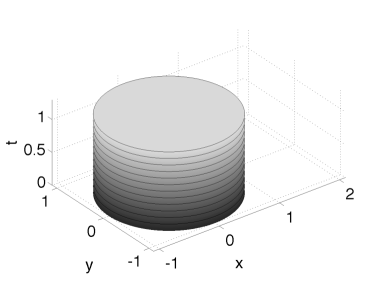
(a) $\mathcal{K}_{0}$

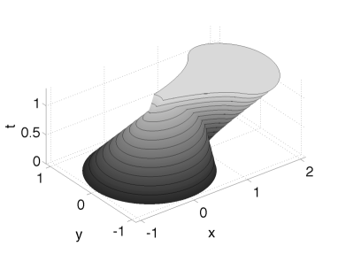
(b) $\mathcal{D}_{x,0}$

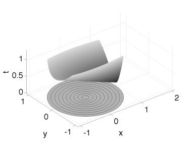
(c) $X^{-1}(\mathcal{C}_{x})$ and $K_{0}$

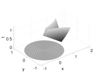
(d) $\mathcal{C}_{x}$ and $K_{0}$

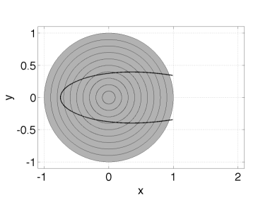
(e) $\mathcal{K}_{0}$ and $X^{-1}(\mathcal{C}_{x})$ at $t=0.8$

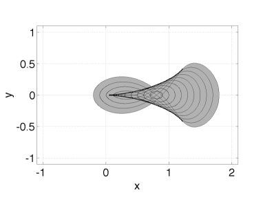
(f) $\mathcal{D}_{x,0}$ and $\mathcal{C}_{x}$ at $t=0.8$

Fig. 1: Examples of the the various sets used in this section for a two-dimensional case, where $\varphi_{0}(x,y)=-x+y^{2}+0.4\,x^{2}$, $T=1.2$ and $K_{0}$ is the unit circle. In the last row the intersection of the sets with the plane $t=0.8$ is shown; the solid black line indicates $X^{-1}({\mathcal{C}}_{x})$ and ${\mathcal{C}}_{x}$ respectively.

The total caustic set $\mathcal{C}_{\delta}$ and domain $\mathcal{D}_{\delta}$ are finally defined as the union of the corresponding sets of each mode,

$$\mathcal{C}_{\delta}=\begin{cases}\mathcal{C}_{x,\delta},&\text{Schr\"{o}dinger},\\ \mathcal{C}_{x^{+},\delta}\cup\mathcal{C}_{x^{-},\delta},&\text{wave equation},\end{cases}\qquad\mathcal{D}_{\delta}=\begin{cases}\mathcal{D}_{x,\delta},&\text{Schr\"{o}dinger},\\ \mathcal{D}_{x^{+},\delta}\cup\mathcal{D}_{x^{-},\delta},&\text{wave equation}.\end{cases}$$

Note that for the wave equation an equivalent definition of $\mathcal{C}_{\delta}$ is the $\delta$-fattened version of $\mathcal{C}_{x^{+}}\cup\mathcal{C}_{x^{-}}$. Moreover, we always consider $[0,T]\times\mathbb{R}^{n}$ to be the universal set and complements of sets are taken with respective to this, i.e. for ${\mathcal{U}}\subset[0,T]\times\mathbb{R}^{n}$,

$${\mathcal{U}}^{c}=[0,T]\times\mathbb{R}^{n}\setminus{\mathcal{U}}.$$

Finally, in the proofs we will typically not use property (P4) the way it is written in Lemma 2, but rather the following simple consequence, which we denote (P$4^{\prime}$),

• there exists a constant $w_{4}>0$ such that

  $$\left|e^{i\Phi(t,y,z)/\varepsilon}\varrho_{\eta}(y)\right|\leq e^{-w_{4}|y|^{2}/\varepsilon},$$

  for all $(t,z)\in{\mathcal{K}}_{d}$ and $y\in\mathbb{R}^{n}$.

Remark 6.1.

Note that the caustic set is fattened both in space and time. This is necessary for the estimates derived below to be true; the rate $\varepsilon^{\lceil k/2\rceil}$ is only obtained uniformly away from the caustics, in space and time.

6.2 Main Result

We are now ready to state the main theorem of this section. It gives max norm error estimates in terms of $\varepsilon$, over different parts of the solution domain. The theorem shows that uniformly away from caustics, $(t,y)\in{\mathcal{C}}^{c}_{\delta}$, the convergence rate is the same $O(\varepsilon^{k/2})$ as in [26] when $k$ is even. For odd $k$, however, error cancellations between adjacent beams can be exploited, and the better rate $O(\varepsilon^{(k+1)/2})$ is obtained, similar to the results in [41, 29]. We believe this rate is sharp. Close to a caustic point, $(t,y)\in{\mathcal{C}}_{\delta}$, the theorem gives the rather coarse rate estimate $O(\varepsilon^{(k-n)/2})$, which can likely be improved for many types of caustics. Finally, away from the essential support of the solution, $(t,y)\in{\mathcal{D}}_{\delta}^{c}$, the convergence is exponential in $\varepsilon$. In fact, the solution itself is also exponentially small in $\varepsilon$ on this domain.

Theorem 10.

Let $u_{k}$ be the $k$-th order Gaussian beam superposition given in Section 3 for the Schrödinger equation (1) or the wave equation (2), with a cutoff width $\eta$ that is admissible for $K_{d}$, $T>0$ and the correspondning Gaussian beam phases, $\Phi_{k}$ or $\Phi^{\pm}_{k}$. If $u$ is the exact solution to Schrödinger’s equation or the wave equation, then we have the following estimate. For each $\delta>0$ and $m>0$, there is a constant $C_{\delta,m}$ such that

$${}|u_{k}(t,y)-u(t,y)|\leq C_{\delta,m}\begin{cases}\varepsilon^{\lceil k/2\rceil},&(t,y)\in{\mathcal{C}}^{c}_{\delta},\\ \varepsilon^{(k-n)/2},&(t,y)\in{\mathcal{C}}_{\delta},\\ \varepsilon^{m},&(t,y)\in{\mathcal{D}}^{c}_{\delta},\end{cases}\qquad\forall\varepsilon\in(0,1].$$ (43)

The theorem also immediately gives us an estimate for the initial data in all $L_{p}$-norms.

Corollary 11.

Under the same conditions as in Theorem 10, there is a constant $C_{p}$ for each $1\leq p\leq\infty$ such that

$${}||u_{k}(0,y)-u(0,y)||_{L^{p}(\mathbb{R}^{n})}\leq C_{p}\varepsilon^{\lceil k/2\rceil},\qquad 1\leq p\leq\infty,\quad\forall\varepsilon\in(0,1].$$ (44)

Proof.

Since $x(0,z)=z$ and $K_{d}$ is compact, there exists $\delta>0$ such that $\det J(t,z)\neq 0$ for $t\in[0,\delta]$ and $z\in K_{d}$. Hence, there is a caustic free initial interval $[0,\delta]$ and for $T=\delta$, the fattened caustic set ${\mathcal{C}}_{\delta}$ is empty. Theorem 10 then shows that there is a constant $C$ such that for all $\varepsilon\in(0,1]$.

$$|u_{k}(t,y)-u(t,y)|\leq C\varepsilon^{\lceil k/2\rceil},\qquad\forall(t,y)\in[0,\delta]\times\mathbb{R}^{n}.$$

Since initial data for both $u_{k}$ and $u$ is compactly supported, the result extends to all $L_{p}$-norms at $t=0$. ∎

We prove Theorem 10 starting from a standard Sobolev inequality and the result in the previous section, namely

$${}\sup_{t\in[0,T]}||u(t,\,\cdot\,)-u_{k}(t,\,\cdot\,)||_{L^{\infty}(\mathbb{R}^{n})}\leq C\sup_{t\in[0,T]}||u(t,\,\cdot\,)-u_{k}(t,\,\cdot\,)||_{H^{s}(\mathbb{R}^{n})}\leq C\varepsilon^{\frac{k}{2}-s},$$ (45)

for any $s>n/2$, and $s\geq 1$ for the wave equation. We take $s=\lfloor n/2\rfloor+1$ to ensure this. The estimate (45) is rather pessimistic. However, we can improve it by using the fact that better estimates can be proved for the difference between beams of different orders. Let $p=2\lfloor n/2\rfloor+3+m^{\prime}=2s+1+m^{\prime}$ where $m^{\prime}\in\mathbb{Z}^{+}$ and $m^{\prime}\geq\max(2m-k-1,0)$. Assume that $\eta$ is admissible also for $K_{d}$, $T$ and the higher order Gaussian beam phase $\Phi_{k+p}$, for the Schrödinger equation, or $\Phi^{\pm}_{k+p}$ for the wave equation. Then, by (45)

$${}|u(t,y)-u_{k}(t,y)| \leq||u(t,\,\cdot\,)-u_{k+p}(t,\,\cdot\,)||_{L^{\infty}(\mathbb{R}^{n})}+|u_{k+p}(t,y)-u_{k}(t,y)|$$

$$\leq C\varepsilon^{(k+p)/2-s}+|u_{k+p}(t,y)-u_{k}(t,y)|,$$ (46)

for $(t,y)\in[0,T]\times\mathbb{R}^{n}$. We now need to use a representation result similiar to Lemma 5 showing that the difference between beams of different orders can be written as a sum of oscillatory integrals of the type (34), but where the property (P5) is replaced by three new properties, namely:

• $\Phi(t,0,z)$ and $\nabla_{y}\Phi(t,0,z)$ are real and

  $${}J(t,z)^{T}\nabla_{y}\Phi(t,0,z)=\nabla_{z}\Phi(t,0,z),$$ (47)

  for all $t\geq 0$ and $z\in\mathbb{R}^{n}$.

• $g(t,y,z,\varepsilon)\in L^{\infty}([0,T]\times\mathbb{R}^{n}\times{K}_{d}\times\mathbb{R}^{+})$ is compactly supported in $K_{0}$ for fixed $(t,y,\varepsilon)$, and there are positive constants $D_{7}$, $w_{7}$, such that for all $(t,z)\in{\mathcal{K}}_{d}$, $\varepsilon>0$ and $y\in\mathbb{R}^{n}$,

  $${}\left|g(t,y,z,\varepsilon)e^{i\Phi(t,y-x(t,z),z)/\varepsilon}\varrho_{\eta}(y-x(t,z))\right|\leq D_{7}e^{-w_{7}|y-x(t,z)|^{2}/\varepsilon},$$ (48)

• when $y_{0}=x(t,z_{0})$, there are positive constants $D_{8}$, $w_{8}$, such that for all $t\in[0,T]$, $z,z_{0}\in K_{d}$, $\varepsilon>0$ and $y_{0}\in\mathbb{R}^{n}$,

  $$\left|\Bigl{(}g(t,y_{0},z,\varepsilon)-g(t,y_{0},z_{0},\varepsilon)\Bigr{)}e^{i\Phi(t,y_{0}-x(t,z),z)/\varepsilon}\varrho_{\eta}(y_{0}-x(t,z))\right|$$

  $$\leq D_{8}|z-z_{0}|\left(1+\frac{|z-z_{0}|^{q}}{\varepsilon^{\ell}}\right)e^{-w_{8}|y_{0}-x(t,z)|^{2}/\varepsilon},$$ (49)

  with $q\geq 2\ell$.

We are then able to prove the following theorem.

Theorem 12.

Let $u_{k}$ and $u_{k+p}$ be the $k$-th and $(k+p)$-th order Gaussian beam superpositions given in Section 3 for the Schrödinger equation (1) or the wave equation (2). Suppose the same cutoff width $\eta$ is used for both $u_{k}$ and $u_{k+p}$. Then there is a finite $J$ such that

$${}u_{k+p}(t,y)-u_{k}(t,y)=\varepsilon^{\frac{k}{2}}\sum_{j=0}^{J}\varepsilon^{\ell_{j}}\mathcal{I}^{\beta_{j}}_{\Psi_{j},x_{j},g_{j}}(t,y),$$ (50)

where $(\Psi_{j},x_{j})$ is one of $(\Phi_{k},x)$, $(\Phi_{k+p},x)$, for the Schrödinger equation, or $(\Phi^{\pm}_{k},x^{\pm})$, $(\Phi^{\pm}_{k+p},x^{\pm})$, for the wave equation. Moreover, $\ell_{j}\geq 0$ and when $\ell_{j}=0$, the parity (odd/even) of $|\beta_{j}|$ is the same as that of $k$.

In addition, if $\eta$ is admissible for $K_{d}$, $T>0$ and the corresponding Gaussian beam phases, $\Phi_{k}$, $\Phi_{k+p}$, for the Schrödinger equation, or $\Phi^{\pm}_{k}$, $\Phi^{\pm}_{k+p}$, for the wave equation, then each triplet $(\Psi_{j},x_{j},g_{j})$ have properties (P1)–(P4) and (P6)–(P8).

Applying Theorem 12 to (6.2) yields for $t\in[0,T]$,

$${}|u(t,y)-u_{k}(t,y)|\leq C\varepsilon^{(k+1+m^{\prime})/2}+\varepsilon^{\frac{k}{2}}\sum_{j=0}^{J}\varepsilon^{\ell_{j}}\left|\mathcal{I}^{\beta_{j}}_{\Psi_{j},x_{j},g_{j}}(t,y)\right|,$$ (51)

where we used the fact that $(k+p)/2-s=(k+1+m^{\prime})/2$. The last piece needed to prove Theorem 10 is a pointwise estimate of $\mathcal{I}^{\alpha}_{\Phi,x,g}(t,y)$, which is contained in the final theorem of this section,

Theorem 13.

If $(\Phi,x,g)$ have properties (P1)–(P4) and (P6)–(P8), then, for each $\delta>0$ there are constants $C_{\delta}$ and $w_{\delta}>0$ such that

$${}\left|\mathcal{I}^{\alpha}_{\Phi,x,g}(t,y)\right|\leq C_{\delta}\begin{cases}1,&\text{\rm$|\alpha|$ even, $(t,y)\in{\mathcal{C}}^{c}_{x,\delta}$},\\ \varepsilon^{1/2},&\text{\rm$|\alpha|$ odd, $(t,y)\in{\mathcal{C}}^{c}_{x,\delta}$},\\ \varepsilon^{-n/2},&(t,y)\in{\mathcal{C}}_{x,\delta},\\ \exp(-w_{\delta}/\varepsilon),&(t,y)\in{\mathcal{D}}^{c}_{x,\delta},\end{cases}$$ (52)

for all $\varepsilon\in(0,1]$. The constants $C_{\delta}$, $w_{\delta}$ depend on $\alpha$, $\Phi$, $x$, $g$.

Using Theorem 13 in (51) we have for $(t,y)\in{\mathcal{C}}^{c}_{\delta}\subset(\cup_{j}{\mathcal{C}}_{x_{j},\delta})^{c}=\cap_{j}{\mathcal{C}}^{c}_{x_{j},\delta}$,

$$\varepsilon^{\ell_{j}}\left|\mathcal{I}^{\beta_{j}}_{\Psi_{j},x_{j},g_{j}}(t,y)\right|\leq C\begin{cases}1,&\text{$\ell_{j}=0$ and $k$ even},\\ \varepsilon^{1/2},&\text{$\ell_{j}=0$ and $k$ odd},\\ \varepsilon^{\ell_{j}},&\ell_{j}\geq 1,\end{cases}\leq C\begin{cases}1,&\text{$k$ even},\\ \varepsilon^{1/2},&\text{$k$ odd},\end{cases}$$

since $k$ and $|\beta_{j}|$ have the same parity when $\ell_{j}=0$ and $\varepsilon\in(0,1]$. Therefore,

$$\varepsilon^{\frac{k}{2}}\varepsilon^{\ell_{j}}\left|\mathcal{I}^{\beta_{j}}_{\Psi_{j},x_{j},g_{j}}(t,y)\right|\leq C\varepsilon^{\lceil k/2\rceil},$$

and because $m^{\prime}\geq 0$, the first case in (43) is proved. When $(t,y)\in{\mathcal{D}}^{c}_{\delta}\subset(\cup_{j}{\mathcal{D}}_{x_{j},\delta})^{c}=\cap_{j}{\mathcal{D}}^{c}_{x_{j},\delta}$, the second term in (51) is asymptotically smaller than all powers of $\varepsilon$, so the first term in (51) dominates, irrespective of $m^{\prime}\geq 0$. This shows the third case in (43) since $(k+1+m^{\prime})/2\geq m$. The second case is finally estimated simply by the largest term in Theorem 13. Theorem 10 is thereby proved, if $\eta$ is indeed admissible for the higher order phase $\Phi_{k+p}$ or $\Phi^{\pm}_{k+p}$. If not, let $\tilde{\eta}<\eta$ be an admissible cutoff width for $K_{d}$, $T$ and the higher order phase. Lemma 2 ensures the existence of such $\tilde{\eta}$. Denote by $\tilde{u}_{k}$ and $\tilde{u}_{k+p}$ the Gaussian beam superpositions of orders $k$ and $k+p$ respectively, which (both) use $\tilde{\eta}$ as cutoff width. This width is clearly admissible for both of them and therefore the theorem holds for $\tilde{u}_{k}$. Moreover, by Lemma 4, the difference $|u_{k}-\tilde{u}_{k}|$ is exponentially small in $\varepsilon$, which implies that the theorem also holds for $u_{k}$.

The remainder of this section is dedicated to proving Theorem 12 and Theorem 13.

6.3 Proof of Theorem 12

As we will show below, the Gaussian beam phase $\Psi_{j}$ of the oscillatory integrals in (50) is always one of $\Phi_{k}$, $\Phi_{k+p}$, for the Schrödinger equation, and one of $\Phi^{\pm}_{k}$, $\Phi^{\pm}_{k+p}$, for the wave equation. All these phases, and their corresponding central rays $x$, $x^{\pm}$, have properties (P1)–(P4) by Lemma 2, and the assumption on $\eta$. The first step in the proof is a lemma proving that these phases also satisfy (P6).

Lemma 14.

For all $k\geq 0$, property (P6) is true for the Schrödinger phase $\Phi_{k}$ and its central ray $x$, as well as for the phases $\Phi_{k}^{\pm}$ and central rays $x^{\pm}$ of the wave equation.

Proof.

As noted in Remark 3.1, the first three equations in (23) and (25) have the Hamiltonian structure in (26). Let $\phi$ and $H$ represent the phase and Hamiltonian for the Schrödinger equation or one of the modes of the wave equation. Moreover, let $\phi_{0}$, $x$ and $p$ be the corresponding phase, central ray and ray direction. They are well-defined for all $t\geq 0$ and $z\in\mathbb{R}^{n}$ by the discussion in Section 4.1. They are also real, since the initial data (27) is real and $H(x,p)$ is real whenever $x$ and $p$ are real. The first part of (P6) is then proved by noting that $\phi(t,0,z)=\phi_{0}(t,z)$ and $\nabla\phi(t,0,z)=p(t,z)$. Next, let $J(t,z)=D_{z}x(t,z)$ and define

$$S(t,z):=J(t,z)^{T}\nabla_{y}\phi(t,0,z)-\nabla_{z}\phi(t,0,z)=J(t,z)^{T}p(t,z)-\nabla_{z}\phi_{0}(t,z),$$

which is zero at $t=0$ by (27). From (26), with $P(t,z)=D_{z}p(t,z)$, it then follows that

$$\partial_{t}S =(D_{z}\partial_{t}x)^{T}p+J^{T}\partial_{t}p-\nabla_{z}\partial_{t}\phi_{0}$$

$$=(D_{z}\nabla_{p}H)^{T}p-J^{T}\nabla_{y}H-\nabla_{z}(-H+(\nabla_{p}H)^{T}p)$$

$$=(D_{z}\partial_{p}H)^{T}p-J^{T}\nabla_{y}H+J^{T}\nabla_{y}H+P^{T}\nabla_{p}H-(D_{z}\nabla_{p}H)^{T}p-P^{T}\nabla_{p}H=0.$$

This shows that $S$ is zero for all times, which proves the lemma. ∎

We will now continue with the proof for the Schrödinger case. Since the wave equation beams are just sums of beams for its two modes, the proof for the wave equation case will be identical, and we leave it out.

By (15) we have for the Schrödinger equation

$$u_{k+p}(t,y)-u_{k}(t,y)=\left(\frac{1}{2\pi\varepsilon}\right)^{\frac{n}{2}}\int_{K_{0}}[v_{k+p}(t,y,z)-v_{k}(t,y,z)]\varrho_{\eta}(y-x(t,z))dz,$$

since the same $\eta$ is used for the $k$-th and the $(k+p)$-th order beams.

Starting from the expressions for $\Phi_{k}$ and $A_{k}$ in (12) and (13, 14) we can analyze the differences $v_{k+p}-v_{k}$. We obtain

$${}v_{k+p}-v_{k} =A_{k+p}e^{i\Phi_{k+p}/\varepsilon}-A_{k}e^{i\Phi_{k}/\varepsilon}$$

$$=\left(A_{k+p}-A_{k}\right)e^{i\Phi_{k+p}/\varepsilon}+A_{k}\left(e^{i\Phi_{k+p}/\varepsilon}-e^{i\Phi_{k}/\varepsilon}\right).$$ (53)

By the discussion in Section 4.1 none of $x$, $p$, $\phi_{0}$, $M$, $\phi_{\beta}$ or $a_{j,\beta}$ depend on $k$. Therefore,

$$A_{k+p}(t,y,z)-A_{k}(t,y,z) =\sum_{j=0}^{\lceil\frac{k}{2}\rceil-1}\varepsilon^{j}\left[\bar{a}_{j,k+p}(t,y,z)-\bar{a}_{j,k}(t,y,z)\right]$$

$$\mbox{\ \ \ }+\sum_{j=\lceil\frac{k}{2}\rceil}^{\lceil(k+p)/2\rceil-1}\varepsilon^{j}\bar{a}_{j,k+p}(t,y,z)$$

$$=\sum_{j=0}^{\lceil\frac{k}{2}\rceil-1}\sum_{|\beta|=k-2j}^{k+p-2j-1}\frac{1}{\beta!}a_{j,\beta}(t,z)\varepsilon^{j}y^{\beta}$$

$$\mbox{\ \ \ }+\sum_{j=\lceil\frac{k}{2}\rceil}^{\lceil(k+p)/2\rceil-1}\sum_{|\beta|=0}^{k+p-2j-1}\frac{1}{\beta!}a_{j,\beta}(t,z)\varepsilon^{j}y^{\beta}.$$

This is a finite sum of terms having the form $a_{j,\beta}(t,z)\varepsilon^{j}y^{\beta}/\beta!$. It can easily be checked that $j+|\beta|/2\geq\frac{k}{2}$ for all terms. Therefore, for some finite $N_{a}$, functions $g_{j}$, multi-indices $\alpha_{j}$ and powers $\ell_{j}\geq 0$, we can write the sum as

$$A_{k+p}(t,y,z)-A_{k}(t,y,z)=\varepsilon^{\frac{k}{2}}\sum_{j=0}^{N_{a}}\varepsilon^{\ell_{j}-|\alpha_{j}|/2}g_{j}(t,z)y^{\alpha_{j}},$$

where the $g_{j}$ functions are equal to scaled amplitude coefficients, which satisfy (30) and (31). Moreover, if $\ell_{j}=0$ then $|\alpha_{j}|=k-2j$, so $|\alpha_{j}|$ then has the same parity as $k$. In (6.3) the amplitudes and phases are evaluated at $y-x(t,z)$ and hence, the first term there contributes to $u_{k+p}-u_{k}$ as

$${}\left(\frac{1}{2\pi\varepsilon}\right)^{\frac{n}{2}}\int_{K_{0}}\left(A_{k+p}-A_{k}\right)e^{i\Phi_{k+p}/\varepsilon}\varrho_{\eta}dz=\varepsilon^{\frac{k}{2}}\sum_{j=0}^{N_{a}}\varepsilon^{\ell_{j}}\mathcal{I}^{\alpha_{j}}_{\Phi_{k+p},x,g_{j}},$$ (54)

where $|\alpha_{j}|$ has the same parity as $k$ when $\ell_{j}=0$. For this case the $g_{j}$ functions are independent of both $y$ and $\varepsilon$, and by (31) they have supp $g_{j}\subset K_{0}$. Therefore, by (30) and (7), property (P$4^{\prime}$) implies (P7) and (P8), with $w_{7}=w_{8}=w_{4}$ and

$$D_{7}=\sup_{t\in[0,T]}||g_{j}(t,\,\cdot\,)||_{L^{\infty}(K_{d})},\quad D_{8}=\sup_{t\in[0,T]}|g_{j}(t,\,\cdot\,)|_{{\rm Lip}(K_{d})},\quad q=\ell=0.$$

We conclude that the oscillatory integrals in (54) all satisfy (P1)–(P4) and (P6)–(P8).

We now consider the second term in (6.3) and define the function

$${}\tilde{g}(t,y,z,\varepsilon):=\int_{0}^{1}e^{is(\Phi_{k+p}(t,y,z)-\Phi_{k}(t,y,z))/\varepsilon}ds.$$ (55)

By (30) we have $\tilde{g}(t,y,z,\varepsilon)\in C^{\infty}([0,T]\times\mathbb{R}^{n}\times{K}_{d}\times\mathbb{R}^{+})$. A simple calculation shows that

$$e^{i\Phi_{k+p}/\varepsilon}-e^{i\Phi_{k}/\varepsilon}=\left(e^{i(\Phi_{k+p}-\Phi_{k})/\varepsilon}-1\right)e^{i\Phi_{k}/\varepsilon}=\frac{i}{\varepsilon}\tilde{g}(\Phi_{k+p}-\Phi_{k})e^{i\Phi_{k}/\varepsilon}.$$

Then we have

$$A_{k}(t,y,z)\left(e^{i\Phi_{k+p}(t,y,z)/\varepsilon}-e^{i\Phi_{k}(t,y,z)/\varepsilon}\right)$$

$$=\frac{i}{\varepsilon}\tilde{g}(t,y,z,\varepsilon)A_{k}(t,y,z)\Bigl{(}\Phi_{k+p}(t,y,z)-\Phi_{k}(t,y,z)\Bigr{)}e^{i\Phi_{k}(t,y,z)/\varepsilon}$$

$$=\frac{i}{\varepsilon}\tilde{g}(t,y,z,\varepsilon)A_{k}(t,y,z)\sum_{|\beta|=k+2}^{k+p+1}\frac{1}{\beta!}\phi_{\beta}(t,z)y^{\beta}e^{i\Phi_{k}(t,y,z)/\varepsilon}$$

$$=i\tilde{g}(t,y,z,\varepsilon)e^{i\Phi_{k}(t,y,z)/\varepsilon}\sum_{j=0}^{\lceil\frac{k}{2}\rceil-1}\sum_{|\beta_{1}|=0}^{k-2j-1}\sum_{|\beta_{2}|=k+2}^{k+p+1}\frac{\varepsilon^{j-1}}{\beta_{1}!\beta_{2}!}a_{j,\beta_{1}}(t,z)\phi_{\beta_{2}}(t,z)y^{\beta_{1}+\beta_{2}}.$$

As before, this is a finite sum, now with terms of the form

$${}i\tilde{g}(t,y,z,\varepsilon)\frac{\varepsilon^{j-1}}{\beta_{1}!\beta_{2}!}a_{j,\beta_{1}}(t,z)\phi_{\beta_{2}}(t,z)y^{\beta_{1}+\beta_{2}}e^{i\Phi_{k}(t,y,z)/\varepsilon}.$$ (56)

It is again easy to check that $j-1+|\beta_{1}+\beta_{2}|/2\geq k/2$ for all terms. There are therefore functions $g_{j}$, multi-indices $\alpha_{j}$ and powers $\ell_{j}\geq 0$ such that for some finite $N_{q}$,

$$A_{k}\left(e^{i\Phi_{k+p}/\varepsilon}-e^{i\Phi_{k}/\varepsilon}\right)=\varepsilon^{\frac{k}{2}}\sum_{j=0}^{N_{q}}\varepsilon^{\ell_{j}-|\alpha_{j}|/2}g_{j}(t,y,z,\varepsilon)(y-x(t,z))^{\alpha_{j}}e^{i\Phi_{k}(t,y-x(t,z),z)/\varepsilon},$$

where $|\alpha_{j}|=k-2j+2$ if $\ell_{j}=0$, so, again, $|\alpha_{j}|$ then has the same parity as $k$. Hence, the second term in (6.3) contributes to $u_{k+p}-u_{k}$ as

$${}\left(\frac{1}{2\pi\varepsilon}\right)^{\frac{n}{2}}\int_{K_{0}}A_{k}\left(e^{i\Phi_{k+p}/\varepsilon}-e^{i\Phi_{k}/\varepsilon}\right)\varrho_{\eta}dz=\varepsilon^{\frac{k}{2}}\sum_{j=0}^{N_{q}}\varepsilon^{\ell_{j}}\mathcal{I}^{\alpha_{j}}_{\Phi_{k},x,g_{j}},$$ (57)

where, as before, $\Phi_{k}$ and $x$ have properties (P1)–(P4) and (P6).

We have left to prove that $\Phi_{k}$, $x$, and $g_{j}$ have properties (P7) and (P8). By (56), (30) and (31), each $g_{j}$ is of the form $f_{j}(t,z)\tilde{g}(t,y-x(t,z),z,\varepsilon)$ where $f_{j}(t,z)\in C^{\infty}({\mathcal{K}}_{d})$ and supp$f_{j}(t,\,\cdot\,)\subset K_{0}$ for $t\in[0,T]$. Hence, $g_{j}(t,y,z,\varepsilon)\in C^{\infty}([0,T]\times\mathbb{R}^{n}\times{K}_{d}\times\mathbb{R}^{+})$, with compact support in $K_{0}$ for fixed $t,y,\varepsilon$.

To show (48) and ((P8)), we note first that since both the phases $\Phi_{k}$, $\Phi_{k+p}$ satisfy (P$4^{\prime}$), we have for any $s\in[0,1]$, $(t,z)\in{\mathcal{K}}_{d}$, $y\in\mathbb{R}^{n}$ and $\varepsilon>0$,

$${}\left|e^{i[s\Phi_{k+p}(t,y,z)+(1-s)\Phi_{k}(t,y,z)]/\varepsilon}\varrho_{\eta}(y)\right| =e^{-s\Im\Phi_{k+p}(t,{y},z)-(1-s)\Im\Phi_{k}(t,{y},z)]/\varepsilon}\varrho_{\eta}(y)$$

$$\leq e^{-sw_{4,k+p}|{y}|^{2}/\varepsilon-(1-s)w_{4,k}|{y}|^{2}/\varepsilon}$$

$$\leq e^{-\tilde{w}_{4}|y|^{2}},$$ (58)

where $w_{4,\ell}$ is the constant in (P$4^{\prime}$) for $\Phi_{\ell}$ and $\tilde{w}_{4}=\min(w_{4,k+p},w_{4,k})$. To simplify the presentation in the remainder of the proof, we let $\tilde{y}=y_{0}-x(t,z)$ and drop the index $j$ from $g_{j}$ and $f_{j}$. Then by (6.3) and (7),

$$\left|g(t,y_{0},z,\varepsilon)e^{i\Phi_{k}(t,y_{0}-x(t,z),z)/\varepsilon}\varrho_{\eta}(y_{0}-x(t,z))\right|$$

$$=\left|f(t,z)\tilde{g}(t,\tilde{y},z,\varepsilon)e^{i\Phi_{k}(t,\tilde{y},z)/\varepsilon}\varrho_{\eta}(\tilde{y})\right|$$

$$=\left|f(t,z)\int_{0}^{1}e^{i[s\Phi_{k+p}(t,\tilde{y},z)+(1-s)\Phi_{k}(t,\tilde{y},z)]/\varepsilon}\varrho_{\eta}(\tilde{y})ds\right|\leq C_{1}e^{-{\tilde{w}}_{4}|\tilde{y}|^{2}/\varepsilon},$$

for all $(t,z)\in{\mathcal{K}}_{d}$. This shows (48) and therefore (P7) with $D_{7}=C_{1}$ and $w_{7}=\tilde{w}_{4}$.

Finally, for ((P8)) we use the fact that $\Phi_{k}(t,0,z)=\Phi_{k+p}(t,0,z)=\phi_{0}(t,z)$, which means that $\tilde{g}(t,0,z,\varepsilon)=1$. We can therefore split

$$\Bigl{(}g(t,y_{0},z,\varepsilon)-g(t,y_{0},z_{0},\varepsilon)\Bigr{)}e^{i\Phi_{k}(t,y_{0}-x(t,z),z)/\varepsilon}\varrho_{\eta}(y_{0}-x(t,z))$$

$$=\Bigl{(}f(t,z)\tilde{g}(t,\tilde{y},z,\varepsilon)-f(t,z_{0})\tilde{g}(t,0,z_{0},\varepsilon)\Bigr{)}e^{i\Phi_{k}(t,\tilde{y},z)/\varepsilon}\varrho_{\eta}(\tilde{y})$$

$$=f(t,z)\Bigl{(}\tilde{g}(t,\tilde{y},z,\varepsilon)-1\Bigr{)}e^{i\Phi_{k}(t,\tilde{y},z)/\varepsilon}\varrho_{\eta}(\tilde{y})+\Bigl{(}f(t,z)-f(t,z_{0})\Bigr{)}e^{i\Phi_{k}(t,\tilde{y},z)/\varepsilon}\varrho_{\eta}(\tilde{y}).$$

Since $f$ is smooth, $t\in[0,T]$ and $z,z_{0}\in K_{d}$, it follows from (7) and (P$4^{\prime}$) that the second term can be estimated as

$${}\left|(f(t,z)-f(t,z_{0}))e^{i\Phi_{k}(t,\tilde{y},z)/\varepsilon}\varrho_{\eta}(\tilde{y})\right|\leq C_{2}|z-z_{0}|e^{-w_{4,k}|\tilde{y}|^{2}/\varepsilon}.$$ (59)

For the first term we consider

$$\Bigl{(}\tilde{g}(t,\tilde{y},z,\varepsilon)-1\Bigr{)}e^{i\Phi_{k}(t,\tilde{y},z)/\varepsilon}$$

$$=\int_{0}^{1}\left(e^{is(\Phi_{k+p}(t,\tilde{y},z)-\Phi_{k}(t,\tilde{y},z))/\varepsilon}-1\right)ds\times e^{i\Phi_{k}(t,\tilde{y},z)/\varepsilon}$$

$$=\frac{i}{\varepsilon}(\Phi_{k+p}(t,\tilde{y},z)-\Phi_{k}(t,\tilde{y},z))\int_{0}^{1}\int_{0}^{1}se^{i(sr\Phi_{k+p}(t,\tilde{y},z)+(1-sr)\Phi_{k}(t,\tilde{y},z))/\varepsilon}dsdr.$$

Hence, upon again using (6.3), (30) and (7),

$$\left|f(t,z)\Bigl{(}\tilde{g}(t,\tilde{y},z,\varepsilon)-1\Bigr{)}e^{i\Phi_{k}(t,\tilde{y},z)/\varepsilon}\varrho_{\eta}(\tilde{y})\right| \leq\frac{C_{1}}{\varepsilon}|\Phi_{k+p}(t,\tilde{y},z)-\Phi_{k}(t,\tilde{y},z)|e^{-\tilde{w}_{4}|\tilde{y}|^{2}/\varepsilon}$$

$$\leq\frac{C_{1}}{\varepsilon}\sum_{|\beta|=k+2}^{k+p+1}\frac{1}{\beta!}|\phi_{\beta,\ell}(t,z)||\tilde{y}|^{|\beta|}e^{-\tilde{w}_{4}|\tilde{y}|^{2}/\varepsilon}$$

$$\leq\frac{C_{1}^{\prime}}{\varepsilon}|\tilde{y}|^{k+2}e^{-\tilde{w}_{4}|\tilde{y}|^{2}/\varepsilon}\leq\frac{C_{3}}{\varepsilon}|z-z_{0}|^{k+2}e^{-\tilde{w}_{4}|\tilde{y}|^{2}/\varepsilon},$$

where we also used the fact that by (7),

$$|\tilde{y}|=|x(t,z_{0})-x(t,z)|\leq C|z-z_{0}|,$$

whenever $t\in[0,T]$ and $z,z_{0}\in K_{d}$. Together with (59) we thus get an estimate of the type ((P8)) with $D_{8}=\max(C_{1},C_{2},C_{3})$, $w_{8}=\tilde{w}_{4}$, $q=k+1$ and $\ell=1$, which satisfy $q\geq 2\ell$ as $k\geq 1$. This completes the proof of Theorem 12.

6.4 Proof of Theorem 13

We henceforth consider a fixed $\delta>0$ and start by proving the two most simple cases in the theorem: when $(t,y)$ is either outside the essential support of the solution, $(t,y)\in{\mathcal{D}}_{x,\delta}^{c}$, or close to a caustic point, $(t,y)\in{\mathcal{C}}_{x,\delta}$. We next consider the most difficult case, when $(t,y)\in{\mathcal{C}}^{c}_{x,\delta}$. In particular, showing the extra $\varepsilon^{1/2}$ factor when $|\alpha|$ is odd, requires careful estimates. To avoid breaking the flow of the arguments we move most of the various lemmas’ proofs to Appendix A.

6.4.1 Cases $(t,y)\in{\mathcal{D}}_{x,\delta}^{c}$ and $(t,y)\in{\mathcal{C}}_{x,\delta}$

For both these cases we make use of the following integral estimate.

Lemma 15.

Let $U\subset\mathbb{R}^{n}$ be a bounded measurable set. Suppose $|y-x(t,z)|\geq a\geq 0$ when $z\in U$ for a fixed $t\in[0,T]$. If $b\geq 0$ and $c>0$ then

$${}\int_{U}|y-x(t,z)|^{b}e^{-c|y-x(t,z)|^{2}/\varepsilon}dz\leq C|U|\varepsilon^{b/2}e^{-ca^{2}/2\varepsilon},$$ (60)

where $C$ only depends on $b$ and $c$; it is independent of $a$, $(t,y)\in[0,T]\times\mathbb{R}^{n}$ and $\varepsilon>0$.

Proof.

When $b=0$ the result is obviously true for $C=1$. When $b>0$ we use the fact that $x^{p}e^{-x}\leq(p/e)^{p}$ for $p>0$ and $x\geq 0$. Then

$$\int_{U}|y-x(t,z)|^{b}e^{-c|y-x(t,z)|^{2}/\varepsilon}dz \leq\int_{U}|y-x(t,z)|^{b}e^{-c|y-x(t,z)|^{2}/2\varepsilon}e^{-ca^{2}/2\varepsilon}dz$$

$$\leq\left(\frac{\varepsilon b}{c}\right)^{b/2}e^{-b/2}e^{-ca^{2}/2\varepsilon}\int_{U}dz.$$

This shows the lemma with $C=\left(b/c\right)^{b/2}e^{-b/2}$. ∎

We now first suppose that $(t,y)\in{\mathcal{D}}_{x,\delta}^{c}$. If $z\in K_{0}$, then by definition

$$|y-x(t,z)|>\delta.$$

Therefore, by (P7) and Lemma 15, with $b=|\alpha|$, $c=w_{7}$ and $a=\delta$,

$$\left|\mathcal{I}^{\alpha}_{\Phi,x,g}(t,y)\right| \leq\varepsilon^{-\frac{n+|\alpha|}{2}}\int_{K_{0}}\left|g(t,y,z,\varepsilon)(y-x(t,z))^{\alpha}e^{i\Phi(t,y-x(t,z),z)/\varepsilon}\varrho_{\eta}(y-x(t,z))\right|dz$$

$$\leq D_{7}\varepsilon^{-\frac{n+|\alpha|}{2}}\int_{K_{0}}|y-x(t,z)|^{|\alpha|}e^{-w_{7}|y-x(t,z)|^{2}/\varepsilon}dz$$

$$\leq D_{7}C|K_{0}|\varepsilon^{-\frac{n}{2}}e^{-w_{7}\delta^{2}/2\varepsilon}\leq C^{\prime}e^{-{w}/\varepsilon},$$

for ${w}<w_{7}\delta^{2}/2$, which proves the case $(t,y)\in{\mathcal{D}}_{x,\delta}^{c}$ since $D_{7}$ and $C$ are uniform constants in $t$ and $y$.

Second, suppose $(t,y)\in{\mathcal{C}}_{x,\delta}$. Here, we simply use Lemma 15 with $a=0$. This does not give an optimal estimate, but slightly better than (45). Hence, by (P7) and Lemma 15 as above, with $b=|\alpha|$, $c=w_{7}$ and $a=0$,

$$\left|\mathcal{I}^{\alpha}_{\Phi,x,g}(t,y)\right| \leq D_{7}\varepsilon^{-\frac{n+|\alpha|}{2}}\int_{K_{0}}|y-x(t,z)|^{|\alpha|}e^{-w_{7}|y-x(t,z)|^{2}/\varepsilon}dz$$

$$\leq D_{7}C|K_{0}|\varepsilon^{-\frac{n}{2}}\leq C^{\prime}\varepsilon^{-\frac{n}{2}},$$

where again $C^{\prime}$ is independent of $(t,y)\in[0,T]\times\mathbb{R}^{n}$. This proves the theorem when $(t,y)\in{\mathcal{C}}_{x,\delta}$.

6.4.2 Case $(t,y)\in{\mathcal{C}}^{c}_{x,\delta}$

This is the most complicated case, in particular when $|\alpha|$ is odd. The key idea of the proof is that the ray function $x(t,z)$ is locally invertible in $z$ on the set ${\mathcal{C}}^{c}_{x,\delta}$. We derive this property from a uniform version of the inverse function theorem; see Theorem 16 below. In order to carefully track the constants in the estimates, and verify that they are independent of $(t,y)\in{\mathcal{C}}^{c}_{x,\delta}$, we define the following, finite, numbers

$${}R_{1}=\mathop{\sup_{t\in[0,T]}}_{z\in{\rm conv}(K_{d})}|J(t,z)|,\qquad R_{2}=\sum_{j=1}^{n}\mathop{\sup_{t\in[0,T]}}_{z\in{\rm conv}(K_{d})}\left|D^{2}_{z}x_{j}(t,z)\right|,$$ (61)

where conv$(K)$ represents the convex hull of $K$ and $x=(x_{1},\ldots,x_{n})^{T}$. This means that whenever $z,z^{\prime}\in K_{d}$ and $t\in[0,T]$,

$$|x(t,z)-x(t,z^{\prime})| \leq R_{1}|z-z^{\prime}|,{}$$ (62)

$$|J(t,z)-J(t,z^{\prime})| \leq R_{2}|z-z^{\prime}|,{}$$ (63)

$$|x(t,z)-x(t,z^{\prime})-J(t,z^{\prime})(z-z^{\prime})| \leq\frac{1}{2}R_{2}|z-z^{\prime}|^{2}.{}$$ (64)

We also define the extended mapping $X:{\mathcal{K}}_{d}\mapsto[0,T]\times\mathbb{R}^{n}$ as

$$X(t,z)=(t,x(t,z)),$$

and we let ${\mathcal{B}}_{r}(z)$ be the open ball of radius $r$ centered at $z$. We then have the following theorem for the ray function $x(t,z)$.

Theorem 16 (Uniform Inverse Function Theorem).

Suppose $d^{\prime}\in(0,d)$ and $\delta^{\prime}>0$. Then there are numbers $R_{-1}$, $\rho>0$ and $0<r\leq d-d^{\prime}$ such that, for all $(t,z_{0})\in{\mathcal{K}}_{d^{\prime}}\setminus X^{-1}({\mathcal{C}}_{x,\delta^{\prime}})$,

• $\bar{\mathcal{B}}_{r}(z_{0})\subset K_{d}$,

• $x(t,\,\cdot\,)$ restricted to ${\mathcal{B}}_{r}(z_{0})$ is a diffeomorphism on its image ${\mathcal{V}}_{r}(t,z_{0}):=x(t,{\mathcal{B}}_{r}(z_{0}))$,

• ${\mathcal{V}}_{r}(t,z_{0})$ is open; if $y_{0}=x(t,z_{0})$, then ${\mathcal{B}}_{\rho}(y_{0})\subset{\mathcal{V}}_{r}(t,z_{0})$, and

• the inverse of the Jacobian $J(t,z)$ is bounded on ${\mathcal{B}}_{r}(z_{0})$,

  $$\sup_{z\in{\mathcal{B}}_{r}(z_{0})}|J^{-1}(t,z)|\leq R_{-1}.$$

Note that $R_{-1}$, $r$ and $\rho$ are uniform in $(t,z_{0})$ but in general depend on $d^{\prime}$ and $\delta^{\prime}$. See (75), (76) and (78) for their precise definitions.

This result follows essentially in the same way as the standard inverse function theorem. For completeness, a proof is given in Appendix A.1.

We let $\{z_{j}\}$ be the set of all solutions in $K_{d/2}$ to the equation $y=x(t,z)$. Since $(t,y)\in{\mathcal{C}}_{x,\delta}^{c}\subset{\mathcal{C}}_{x,\delta/2}^{c}$ all points $(t,z_{j})$ belong to ${\mathcal{K}}_{d/2}\setminus X^{-1}({\mathcal{C}}_{x,\delta/2})$. This set will be used extensively, and we introduce the shorthand notation

$$\bar{\mathcal{K}}:={\mathcal{K}}_{d/2}\setminus X^{-1}({\mathcal{C}}_{x,\delta/2}).$$

We then apply Theorem 16 with the parameters $d^{\prime}=d/2$ and $\delta^{\prime}=\delta/2$, and, henceforth, we let $R_{-1}$, $r$ and $\rho$ be as given by the theorem with these parameters. They then satisfy

$${}0<r\leq d/2,\qquad R_{-1},\rho>0.$$ (65)

We stress that the four bullet points in the theorem are then valid with these numbers for all $(t,z_{0})\in\bar{\mathcal{K}}$.

In the remainder of the proof we will make use of a few consequences of Theorem 16 which we collect in a corollary.

Corollary 17.

The number of solutions $\{z_{j}\}$ in $K_{d/2}$ is bounded by a number $M_{\delta}<\infty$, independently of $(t,y)\in{\mathcal{C}}_{x,\delta}^{c}$. The balls $\{{\mathcal{B}}_{r/2}(z_{j})\}$ are all disjoint. Moreover, if $(t,z_{0})\in\bar{\mathcal{K}}$ and $x(t,z),x(t,z^{\prime})\in{\mathcal{B}}_{\rho}(x(t,z_{0}))$, then

$${}|z-z^{\prime}|\leq R_{-1}|x(t,z^{\prime})-x(t,z)|.$$ (66)

Proof.

If the number of solutions $\{z_{j}\}$ is more than one, suppose $|z_{j}-z_{k}|<r$ for some indices $j,k$. Then $z_{j}\in{\mathcal{B}}_{r}(z_{k})$ and $x(t,z_{j})=x(t,z_{k})$ so $x(t,z)$ is not one-to-one on ${\mathcal{B}}_{r}(z_{k})$. This contradicts the second point of Theorem 16. Hence, $|z_{j}-z_{j}|\geq r$ for all $j\neq k$ and the balls $\{{\mathcal{B}}_{r/2}(z_{j})\}$ are disjoint. Moreover, by the first point in Theorem 16, each disjoint ball ${\mathcal{B}}_{r/2}(z_{j})$ is a subset of $K_{d}$ and their total volume is therefore bounded by the volume of $K_{d}$. The number of solutions must hence be finite, say $M$, and

$$|K_{d}|\geq\sum_{j=1}^{M}|{\mathcal{B}}_{r/2}(z_{j})|=M\omega_{n}(r/2)^{n}\quad\Rightarrow\quad M\leq M_{\delta}=\frac{|K_{d}|2^{n}}{\omega_{n}r^{n}},\qquad\omega_{n}=\frac{\pi^{n/2}}{\Gamma(n/2+1)},$$

where $\omega_{n}$ is the volume of the unit $n$-sphere. This shows the first statement since $M_{\delta}$ only depends on $K_{d}$, $r$ and $n$. For (66) we note that by Theorem 16 there is a smooth inverse $m(t,x)$ satisfying $m(t,x(t,z))=z$ for all $z\in{\mathcal{B}}_{r}(z_{0})$. Let $y_{0}=x(t,z_{0})$. Then

$$|z-z^{\prime}| =|m(t,x(t,z))-m(t,x(t,z^{\prime}))|\leq\sup_{y\in{\mathcal{B}}_{\rho}(y_{0})}\left|D_{x}m(t,y)\right||x(t,z)-x(t,z^{\prime})|$$

$$\leq\sup_{q\in{\mathcal{B}}_{r}(z_{0})}\left|J^{-1}(t,q)\right||x(t,z)-x(t,z^{\prime})|\leq R_{-1}|x(t,z)-x(t,z^{\prime})|.$$

For the last inequality we used the fourth point in Theorem 16. This shows the corollary. ∎

Hence, by Corollary 17 the number of solutions $M$ to $y=x(t,z)$ in $K_{d/2}$ is finite. We define the set $S\subset K_{0}$ as the points away from these solutions $\{z_{j}\}$,

$$S=\begin{cases}K_{0},&M=0,\\ K_{0}\setminus\bigcup_{j=1}^{M}{\mathcal{B}}_{r/2}(z_{j}),&M\geq 0.\end{cases}$$

Since $\{{\mathcal{B}}_{r/2}(z_{j})\}$ are disjoint by Corollary 17 we can then split the integral as

$$\mathcal{I}^{\alpha}_{\Phi,x,g}(t,y) =\varepsilon^{-\frac{n+|\alpha|}{2}}\int_{K_{0}}g(t,y,z,\varepsilon)(y-x(t,z))^{\alpha}e^{i\Phi(t,y-x(t,z),z)/\varepsilon}\varrho_{\eta}(y-x(t,z))dz$$

$$=\int_{S}\cdots\ dz+\sum_{j=1}^{M}\int_{{\mathcal{B}}_{r/2}(z_{j})\cap K_{0}}\cdots\ dz$$

$$=\int_{S}\cdots\ dz+\sum_{j=1}^{M}\int_{{\mathcal{B}}_{r/2}(z_{j})}\cdots\ dz=:I_{S}+\sum_{j=1}^{M}I_{B_{j}}.$$

Here we also used the fact from (P7) that $g(t,y,\,\cdot\,\,,\varepsilon)$ is compactly supported in $K_{0}$. We will show below that there are positive constants $w_{s}$, $C_{S}$ and $C_{B}$ that are independent of $(t,y)\in{\mathcal{C}}^{c}_{x,\delta}$ and $\varepsilon\in(0,1]$ such that

$${}|I_{S}|\leq C_{S}e^{-w_{s}/\varepsilon},\qquad|I_{B_{j}}|\leq C_{B}\begin{cases}1,&\text{$|\alpha|$ is even},\\ \sqrt{\varepsilon},&\text{$|\alpha|$ is odd}.\end{cases}$$ (67)

From Corollary 17 we have that $M$ is bounded by $M_{\delta}$ uniformly in $(t,y)$. We therefore get the desired estimate,

$$\left|\mathcal{I}^{\alpha}_{\Phi,x,g}(t,y)\right| \leq|I_{S}|+M_{\delta}\max_{j}|I_{B_{j}}|\leq C_{S}e^{-w_{s}/\varepsilon}+M_{\delta}C_{B}\begin{cases}1,&\text{$|\alpha|$ is even},\\ \sqrt{\varepsilon},&\text{$|\alpha|$ is odd},\end{cases}$$

$$\leq C\begin{cases}1,&\text{$|\alpha|$ is even},\\ \sqrt{\varepsilon},&\text{$|\alpha|$ is odd},\end{cases}$$

for all $(t,y)\in{\mathcal{C}}^{c}_{x,\delta}$ and $\varepsilon\in(0,1]$.

We now turn to proving (67). It will be done in three steps, one for each case.

Estimate of $I_{S}$.
For this estimate we show that when $z\in S$ then

$$|y-x(t,z)|\geq\bar{\rho}:=\min(\rho,r/2R_{-1},\delta/2).$$

Suppose first that $X(t,z)\not\in{\mathcal{C}}_{x,\delta/2}$. This implies that $(t,z)\in\bar{\mathcal{K}}$ and Theorem 16 applies. Assume $|y-x(t,z)|<\bar{\rho}\leq\rho$. Then $y\in{\mathcal{B}}_{\rho}(x(t,z))$ and by Theorem 16 there is a $z^{\prime}\in{\mathcal{B}}_{r}(z)$ such that $y=x(t,z^{\prime})$. Since $z\in S\subset K_{0}$ and $r\leq d/2$ by (65), we have $z^{\prime}\in K_{d/2}$, so that $z^{\prime}\in\{z_{j}\}$ and $M>0$. Hence, by (66), and the fact that $z\in S$,

$$\frac{r}{2}\leq|z-z^{\prime}|\leq R_{-1}|x(t,z)-x(t,z^{\prime})|<R_{-1}\bar{\rho}\leq\frac{r}{2},$$

a contradiction. So $|y-x(t,z)|\geq\bar{\rho}$ if $X(t,z)\not\in{\mathcal{C}}_{x,\delta/2}$.

Suppose instead that $X(t,z)\in{\mathcal{C}}_{x,\delta/2}$. Then

$$|x(t,z)-y|={\rm dist}(X(t,z),(t,y))\geq{\rm dist}((t,y),{\mathcal{C}}_{x})-{\rm dist}(X(t,z),{\mathcal{C}}_{x})\geq\delta-\delta/2=\delta/2\geq\bar{\rho},$$

since $(t,y)\in{\mathcal{C}}_{x,\delta}^{c}$. We have thus shown that if $z\in S$, then $|y-x(t,z)|\geq\bar{\rho}$. Therefore, by (P7) and Lemma 15, with $C$ and $D_{7}$ independent of $(t,y)$ and $\varepsilon>0$,

$$|I_{S}| =\left|\varepsilon^{-\frac{n+|\alpha|}{2}}\int_{S}g(t,y,z,\varepsilon)(y-x(t,z))^{\alpha}e^{i\Phi(t,y-x(t,z),z)/\varepsilon}\varrho_{\eta}(y-x(t,z))dz\right|$$

$$\leq D_{7}\varepsilon^{-\frac{n+|\alpha|}{2}}\int_{S}|y-x(t,z)|^{|\alpha|}e^{-w_{7}|y-x(t,z)|^{2}/\varepsilon}dz$$

$$\leq D_{7}C\varepsilon^{-\frac{n}{2}}|S|e^{-w_{7}\bar{\rho}^{2}/2\varepsilon}\leq C_{S}e^{-w_{s}/\varepsilon},$$

for $w_{s}<w_{7}\bar{\rho}^{2}/2$. Here we also used the fact that $|S|\leq|K_{0}|<\infty$. This shows the first inequality in (67).

Estimate of $I_{B_{j}}$.
The integrals $I_{B_{j}}$ are all of the form

$$I_{B}(t,z_{0})=\varepsilon^{-\frac{n+|\alpha|}{2}}\int_{{\mathcal{B}}_{\frac{r}{2}}(z_{0})}g(t,y_{0},z,\varepsilon)(y_{0}-x(t,z))^{\alpha}e^{i\Phi(t,y_{0}-x(t,z),z)/\varepsilon}\varrho_{\eta}(y_{0}-x(t,z))dz$$

where $(t,z_{0})\in\bar{\mathcal{K}}$, $y_{0}=x(t,z_{0})$ and the number $r$ is determined from Theorem 16. It follows in particular that ${\mathcal{B}}_{r/2}(z_{0})\subset K_{d}$ so that the estimates in properties (P$4^{\prime}$), (P7) and (P8) can be used. We now need to bound $I_{B}(t,z_{0})$ with constants independent of $(t,z_{0})\in\bar{\mathcal{K}}$ and $\varepsilon\in(0,1]$. For this we use the following lemma.

Lemma 18.

Suppose $r$ is given as above and $y_{0}=x(t,z_{0})$. If $a,b\geq 0$ and $c>0$ there is a constant $C$ such that for all $(t,z_{0})\in\bar{\mathcal{K}}$ and $\varepsilon>0$,

$${}\int_{{\mathcal{B}}_{\frac{r}{2}}(z_{0})}|z-z_{0}|^{a}|y_{0}-x(t,z)|^{b}e^{-c|y_{0}-x(t,z)|^{2}/\varepsilon}dz\leq C\varepsilon^{\frac{n+a+b}{2}}.$$ (68)

The proof is given in Appendix A.2.

Case when $|\alpha|$ even.
For $|\alpha|$ even we directly apply (P7) and Lemma 18 to $I_{B}$ with $a=0$, $b=|\alpha|$ and $c=w_{7}$ to get

$$|I_{B}(t,z_{0})| \leq D_{7}\varepsilon^{-\frac{n+|\alpha|}{2}}\int_{{\mathcal{B}}_{\frac{r}{2}}(z_{0})}|y_{0}-x(t,z)|^{|\alpha|}e^{-w_{7}|y_{0}-x(t,z)|^{2}/\varepsilon}dz\leq C^{\prime}_{B},$$

for all $(t,z_{0})\in\bar{\mathcal{K}}$ and $\varepsilon>0$. This shows the first half of the second estimate in (67).

Case when $|\alpha|$ odd.
In this case we can gain an additional factor of $\varepsilon^{1/2}$ if we make a careful estimate. To do this, we approximate the phase $\Phi$ by its leading order Taylor expansion in $z$ and show that the integral using the approximate $\Phi$ gives negligible contribution to the integral. The following lemma details the phase approximation. It is proved in Appendix A.3.

Lemma 19.

Suppose $r$ is given as above and $y_{0}=x(t,z_{0})$. If the phase $\Phi(t,y,z)$ and central ray $x(t,z)$ have properties (P1)–(P4) and (P6), then there is a bound $R_{3}$ such that for all $(t,z_{0})\in\bar{\mathcal{K}}$ and $z\in{\mathcal{B}}_{r/2}(z_{0})$,

$$\left|\Phi(t,y_{0}-x(t,z),z)-\left(\Phi(t,0,z_{0})+\frac{1}{2}(z-z_{0})^{T}A(t,z_{0})(z-z_{0})\right)\right|\leq R_{3}|z-z_{0}|^{3},$$

where $A(t,z_{0})\in\mathbb{C}^{n\times n}$. The imaginary part of $A$ is symmetric positive definite, and there exists $w_{a}>0$ such that for all $(t,z_{0})\in\bar{\mathcal{K}}$,

$${}\Im{A}(t,z_{0})\geq w_{a}I.$$ (69)

We thus start by approximating $\Phi\approx\tilde{\Phi}$ and $I_{B}\approx\tilde{I}_{B}$ on ${\mathcal{B}}_{r/2}(z_{0})$, where

$$\tilde{\Phi}(t,z,z_{0}):=\Phi(t,0,z_{0})+\frac{1}{2}(z-z_{0})^{T}A(t,z_{0})(z-z_{0}),$$

with $A(t,z_{0})$ as in Lemma 19, and

$$\tilde{I}_{B}(t,z_{0}):=\varepsilon^{-\frac{n+|\alpha|}{2}}\int_{{\mathcal{B}}_{\frac{r}{2}}(z_{0})}g(t,y_{0},z_{0},\varepsilon)(J(t,z_{0})(z_{0}-z))^{\alpha}e^{i\tilde{\Phi}(t,z,z_{0})/\varepsilon}\varrho_{\eta}(y_{0}-x(t,z))dz.$$

We will now show that $\tilde{I}_{B}$ is exponentially small in $\varepsilon$. To do this we use the following lemma describing cancellations occurring in integrals over odd mononomials multiplied by a Gaussian.

Lemma 20.

Let $\alpha$ be an $n$-dimensional multi-index such that $|\alpha|$ is odd. For $A,R\in\mathbb{C}^{n\times n}$ and any $r>0$,

$$\int_{{\mathcal{B}}_{r}(z_{0})}(R(z-z_{0}))^{\alpha}e^{(z-z_{0})^{T}A(z-z_{0})}dz=0.$$

The proof of the lemma is given in Appendix A.4. It shows that the $\tilde{I}_{B}$ integral, without $\varrho_{\eta}$, vanishes, since

$$\int_{{\mathcal{B}}_{\frac{r}{2}}(z_{0})}g(t,y_{0},z_{0},\varepsilon)(J(t,z_{0})(z_{0}-z))^{\alpha}e^{i\tilde{\Phi}(t,z,z_{0})/\varepsilon}dz$$

$$=e^{i\Phi(t,0,z_{0})/\varepsilon}g(t,y_{0},z_{0},\varepsilon)\int_{{\mathcal{B}}_{\frac{r}{2}}(z_{0})}(J(t,z_{0})(z_{0}-z))^{\alpha}e^{\frac{i}{2}(z-z_{0})^{T}A(t,z_{0})(z-z_{0})/\varepsilon}dz=0.$$

Therefore,

$$\tilde{I}_{B}(t,z_{0}) =\varepsilon^{-\frac{n+|\alpha|}{2}}e^{i\Phi(t,0,z_{0})/\varepsilon}g(t,y_{0},z_{0},\varepsilon)$$

$$\ \ \ \times\int_{{\mathcal{B}}_{\frac{r}{2}}(z_{0})}(J(t,z_{0})(z_{0}-z))^{\alpha}e^{\frac{i}{2}(z-z_{0})^{T}A(t,z_{0})(z-z_{0})/\varepsilon}(\varrho_{\eta}(y_{0}-x(t,z))-1)dz.$$

Moreover, $\varrho_{\eta}(y-x)-1$ is identically zero for $|y-x|\leq\eta$, and since $|y_{0}-x(t,z)|=|x(t,z_{0})-x(t,z)|\leq R_{1}|z-z_{0}|$ when $z\in{\mathcal{B}}_{r}(z_{0})$, we have by the positive definiteness of $\Im A$ given in Lemma 19,

$$\left|\int_{{\mathcal{B}}_{\frac{r}{2}}(z_{0})}(J(t,z_{0})(z_{0}-z))^{\alpha}e^{\frac{i}{2}(z-z_{0})^{T}A(t,z_{0})(z-z_{0})/\varepsilon}(\varrho_{\eta}(y_{0}-x(t,z))-1)dz\right|$$

$$\leq\int_{{\mathcal{B}}_{\frac{r}{2}}(z_{0})}|J(t,z_{0})|^{|\alpha|}|z_{0}-z|^{|\alpha|}e^{-\frac{1}{2}(z-z_{0})^{T}\Im A(t,z_{0})(z-z_{0})/\varepsilon}|\varrho_{\eta}(y_{0}-x(t,z))-1|dz$$

$$\leq\left(\frac{R_{1}r}{2}\right)^{|\alpha|}\int_{{\mathcal{B}}_{\frac{r}{2}}(z_{0})}e^{-\frac{w_{a}}{2}|z-z_{0}|^{2}/\varepsilon}|\varrho_{\eta}(y_{0}-x(t,z))-1|dz$$

$$\leq\left(\frac{R_{1}r}{2}\right)^{|\alpha|}\left|{\mathcal{B}}_{\frac{r}{2}}(z_{0})\right|e^{-w_{a}\eta^{2}/R_{1}^{2}2\varepsilon}.$$

Since $\Phi(t,0,z_{0})$ is real by (P6), then by (P7), noting that $y_{0}-x(t,z_{0})=0$,

$${}|g(t,y_{0},z_{0},\varepsilon)|=|g(t,y_{0},z_{0},\varepsilon)e^{i\Phi(t,0,z_{0})/\varepsilon}\varrho_{\eta}(0)|\leq D_{7},$$ (70)

where $D_{7}$ is clearly uniform in $(t,z_{0})$. Hence, there are constants $\tilde{C}_{B}$ and $\tilde{w}$ such that for all $(t,z_{0})\in\bar{\mathcal{K}}$ and $\varepsilon>0$,

$${}|\tilde{I}_{B}(t,z_{0})|\leq\varepsilon^{-\frac{n+|\alpha|}{2}}D_{7}\left(\frac{R_{1}r}{2}\right)^{|\alpha|}\left|{\mathcal{B}}_{\frac{r}{2}}(z_{0})\right|\,e^{-w_{a}\eta^{2}/R_{1}^{2}2\varepsilon}\leq\tilde{C}_{B}e^{-\tilde{w}/\varepsilon},$$ (71)

with $\tilde{w}<w_{a}\eta^{2}/2R_{1}^{2}$.

We next write the difference as

$$\varepsilon^{\frac{n+|\alpha|}{2}}(I_{B}-\tilde{I}_{B})=\int_{{\mathcal{B}}_{\frac{r}{2}}(z_{0})}(E_{1}+E_{2}+E_{3})dz,$$

where

$$E_{1} =[g(t,y_{0},z,\varepsilon)-g(t,y_{0},z_{0},\varepsilon)](y_{0}-x(t,z))^{\alpha}e^{i\Phi(t,y_{0}-x(t,z),z)/\varepsilon}\varrho_{\eta}(y_{0}-x(t,z)),$$

$$E_{2} =g(t,y_{0},z_{0},\varepsilon)[(y_{0}-x(t,z))^{\alpha}-(J(t,z_{0})(z_{0}-z))^{\alpha}]e^{i\Phi(t,y_{0}-x(t,z),z)/\varepsilon}\varrho_{\eta}(y_{0}-x(t,z)),$$

$$E_{3} =g(t,y_{0},z_{0},\varepsilon)(J(t,z_{0})(z_{0}-z))^{\alpha}\left[e^{i\Phi(t,y_{0}-x(t,z),z)/\varepsilon}-e^{i\tilde{\Phi}(t,z,z_{0})/\varepsilon}\right]\varrho_{\eta}(y_{0}-x(t,z)).$$

We will now consider these integrands in sequence.

From (P8) it follows that for all $(t,z_{0})\in\bar{\mathcal{K}}$, $z\in{\mathcal{B}}_{r/2}(z_{0})$ and $\varepsilon>0$,

$${}|E_{1}|\leq D_{8}|z-z_{0}|\left(1+\frac{|z-z_{0}|^{q}}{\varepsilon^{\ell}}\right)|y_{0}-x(t,z)|^{|\alpha|}e^{-w_{8}|y_{0}-x(t,z)|^{2}/\varepsilon},$$ (72)

with $q\geq 2\ell$.

For $E_{2}$ we note first that

$$|a^{\alpha}-b^{\alpha}|=|(a-b+b)^{\alpha}-b^{\alpha}|=\left|\sum_{\stackrel{{\scriptstyle\beta_{1}+\beta_{2}=\alpha}}{{\beta_{2}\neq\alpha}}}\frac{\alpha!}{\beta_{1}!\beta_{2}!}(a-b)^{\beta_{1}}b^{\beta_{2}}\right|\leq\bar{C}(\alpha)\sum_{j=1}^{|\alpha|}|a-b|^{j}|b|^{|\alpha|-j}.$$

Therefore, by using (P$4^{\prime}$), (70) and (64) we get for all $(t,z_{0})\in\bar{\mathcal{K}}$, $z\in{\mathcal{B}}_{r/2}(z_{0})$ and $\varepsilon>0$,

$${}|E_{2}| \leq\bar{C}(\alpha)D_{7}e^{-w_{4}|y_{0}-x(t,z)|^{2}/\varepsilon}\sum_{j=1}^{|\alpha|}|y_{0}-x(t,z)-J(t,z_{0})(z_{0}-z)|^{j}|y_{0}-x(t,z)|^{|\alpha|-j}$$

$$\leq\bar{C}(\alpha)D_{7}\sum_{j=1}^{|\alpha|}\frac{R_{2}^{j}}{2^{j}}|z-z_{0}|^{2j}|y_{0}-x(t,z)|^{|\alpha|-j}e^{-w_{4}|y_{0}-x(t,z)|^{2}/\varepsilon}$$

$$\leq C_{2}\sum_{j=1}^{|\alpha|}|z-z_{0}|^{2j}|y_{0}-x(t,z)|^{|\alpha|-j}e^{-w_{4}|y_{0}-x(t,z)|^{2}/\varepsilon},$$ (73)

where $C_{2}=\bar{C}(\alpha)D_{7}\max(R_{2}/2,(R_{2}/2)^{|\alpha|})$.

For $E_{3}$ we first need to approximate the phase difference factor when $z\in{\mathcal{B}}_{r/2}(z_{0})$ and $(t,z_{0})\in\bar{\mathcal{K}}$. By Lemma 19 and (62),

$$|\Phi-\tilde{\Phi}| \leq R_{3}|z-z_{0}|^{3},$$

$$\Im\tilde{\Phi} =\frac{1}{2}(z-z_{0})^{T}\Im A(t,z_{0})(z-z_{0})\geq\frac{w_{a}|z-z_{0}|^{2}}{2}\geq\frac{w_{a}|y_{0}-x(t,z)|^{2}}{2R_{1}^{2}}.$$

Therefore, upon using (P$4^{\prime}$),

$$\left|e^{i\Phi/\varepsilon}-e^{i\tilde{\Phi}/\varepsilon}\right|\varrho_{\eta} =\left|\frac{i(\Phi-\tilde{\Phi})}{\varepsilon}\int_{0}^{1}e^{i(s\Phi+(1-s)\tilde{\Phi})/\varepsilon}\varrho_{\eta}ds\right|\leq R_{3}\frac{|z-z_{0}|^{3}}{\varepsilon}e^{-\min(\Im\Phi,\Im\tilde{\Phi})/\varepsilon}$$

$$\leq R_{3}\frac{|z-z_{0}|^{3}}{\varepsilon}e^{-\min(w_{4},w_{a}/2R_{1}^{2})|y_{0}-x(t,z)|^{2}/\varepsilon}.$$

Then from (70), with $w^{\prime}=\min(w_{4},w_{a}/2R_{1}^{2})$ and $C_{3}=R_{3}D_{7}R_{1}^{|\alpha|}$,

$${}|E_{3}|\leq\frac{C_{3}}{\varepsilon}|z-z_{0}|^{|\alpha|+3}e^{-w^{\prime}|y_{0}-x(t,z)|^{2}/\varepsilon},$$ (74)

for all $(t,z_{0})\in\bar{\mathcal{K}}$, $z\in{\mathcal{B}}_{r/2}(z_{0})$ and $\varepsilon>0$. We note that all the $E_{j}$ terms can be bounded by a form that can be estimated by Lemma 18. Indeed, if we define

$$U^{\varepsilon}(a,b):=|z-z_{0}|^{a}|y_{0}-x(t,z)|^{b}e^{-c|y_{0}-x(t,z)|^{2}/\varepsilon},\qquad c=\min(w_{8},w^{\prime}),$$

and set $C_{e}=\max(D_{8},C_{2},C_{3})$, we can summarize (72), (6.4.2), (74) as

$$\varepsilon^{\frac{n+|\alpha|}{2}}|I_{B}(t,z_{0})-\tilde{I}_{B}(t,z_{0})|$$

$$\leq C_{e}\int_{{\mathcal{B}}_{\frac{r}{2}}(z_{0})}U^{\varepsilon}(1,|\alpha|)+\frac{1}{\varepsilon^{\ell}}U^{\varepsilon}(q+1,|\alpha|)+\sum_{j=1}^{|\alpha|}U^{\varepsilon}(2j,|\alpha|-j)+\frac{1}{\varepsilon}U^{\varepsilon}(|\alpha|+3,0)dz.$$

We then use Lemma 18, the constant in which we denote $C_{L}$. We get for $0<\varepsilon\leq 1$,

$$\varepsilon^{\frac{n+|\alpha|}{2}}|I_{B}(t,z_{0})-\tilde{I}_{B}(t,z_{0})|$$

$$\leq C_{e}C_{L}\left(\varepsilon^{\frac{n+1+|\alpha|}{2}}+\varepsilon^{\frac{n+q+1-2\ell+|\alpha|}{2}}+\sum_{j=1}^{|\alpha|}\varepsilon^{\frac{n+2j+|\alpha|-j}{2}}+\varepsilon^{\frac{n+|\alpha|+3+0-2}{2}}\right)\leq C^{\prime}\varepsilon^{\frac{n+1+|\alpha|}{2}},$$

since $q\geq 2\ell$. Together with (71) we finally obtain

$$|I_{B}(t,z_{0})|\leq|I_{B}(t,z_{0})-\tilde{I}_{B}(t,z_{0})|+|\tilde{I}_{B}(t,z_{0})|\leq C^{\prime}\sqrt{\varepsilon}+\tilde{C}_{B}e^{-\tilde{w}/\varepsilon}\leq C^{\prime\prime}_{B}\sqrt{\varepsilon},$$

for all $(t,z_{0})\in\bar{\mathcal{K}}$ and $0<\varepsilon\leq 1$. This shows the last part of the second inequality in (67), and completes the proof with $C_{B}=\max(C^{\prime}_{B},C^{\prime\prime}_{B})$.

Appendix A Proofs

A.1 Proof of Theorem 16

The proof essentially follows the standard steps for proving the inverse function theorem; see for instance [35]. We let ${\mathcal{K}}^{\prime}={\mathcal{K}}_{d^{\prime}}\setminus X^{-1}({\mathcal{C}}_{x,\delta^{\prime}})$ and consider the function

$$\phi(z)=z+J^{-1}(t,z_{0})(y-x(t,z)),$$

with $(t,z_{0})\in{\mathcal{K}}^{\prime}$ and $y\in\mathbb{R}^{n}$ fixed. Since $J$ is non-singular on ${\mathcal{K}}^{\prime}$, finding a fixed point $\phi(z)=z$ is equivalent to finding a solution to the equation $y=x(t,z)$. We note that $J$ is non-singular also on the slightly larger set ${\mathcal{K}}^{\prime\prime}={\mathcal{K}}_{d}\setminus X^{-1}({\mathcal{C}}_{x,\delta^{\prime}/2})\supset{\mathcal{K}}^{\prime}$ and we let $R_{-1}$ be an upper bound of $J^{-1}$ on this (compact) set,

$${}R_{-1}=\sup_{(t,z)\in{\mathcal{K}}^{\prime\prime}}|J^{-1}(t,z)|<\infty.$$ (75)

We then choose $r$ as

$${}r=\min\left(d-d^{\prime},\frac{1}{2R_{-1}R_{2}},\frac{\delta^{\prime}}{2R_{1}}\right)>0.$$ (76)

We note that if $z\in\bar{\mathcal{B}}_{r}(z_{0})$ we have

$${\rm dist}(z,K_{0})\leq|z-z_{0}|+{\rm dist}(z_{0},K_{0})\leq r+d^{\prime}\leq d,$$

Hence, $\bar{\mathcal{B}}_{r}(z_{0})\subset K_{d}$ and for $z_{1},z_{2}\in\bar{\mathcal{B}}_{r}(z_{0})$, using (63),

$${}|\phi(z_{1})-\phi(z_{2})| \leq\max_{z\in\bar{\mathcal{B}}_{r}(z_{0})}\left|D\phi(z)\right||z_{1}-z_{2}|=\max_{z\in\bar{\mathcal{B}}_{r}(z_{0})}\left|I-J^{-1}(t,z_{0})J(t,z)\right||z_{1}-z_{2}|$$

$$\leq R_{-1}\max_{z\in\bar{\mathcal{B}}_{r}(z_{0})}\left|J(t,z_{0})-J(t,z)\right||z_{1}-z_{2}|\leq R_{-1}R_{2}|z_{1}-z_{2}||z-z_{0}|$$

$$\leq R_{-1}R_{2}r|z_{1}-z_{2}|\leq\frac{1}{2}|z_{1}-z_{2}|.$$ (77)

If $z_{1}$ and $z_{2}$ are both, different, fixed points of $\phi$ we get an impossible inequality. It follows that $\phi$ has at most one fixed point in $\bar{\mathcal{B}}_{r}(z_{0})$ and therefore $x(t,z)$ is one-to-one on $\bar{\mathcal{B}}_{r}(z_{0})$. We next show that ${\mathcal{V}}_{r}(t,z_{0})$ is open. For each $y^{\prime}\in{\mathcal{V}}_{r}(t,z_{0})$ there is a $z^{\prime}\in{\mathcal{B}}_{r}(z_{0})$ and a $\lambda>0$, such that $y^{\prime}=x(t,z^{\prime})$ and ${B}_{\lambda}(z^{\prime})\subset{\mathcal{B}}_{r}(z_{0})$. Let $\lambda^{\prime}=\lambda/2R_{-1}$. Then if $y\in{\mathcal{B}}_{\lambda^{\prime}}(y^{\prime})$,

$$|\phi(z^{\prime})-z^{\prime}| =\left|J^{-1}(t,z_{0})(y-y^{\prime})\right|\leq R_{-1}|y-y^{\prime}|<R_{-1}\lambda^{\prime}=\frac{1}{2}\lambda.$$

Consequentially, by (A.1), if $z\in\bar{\mathcal{B}}_{\lambda}(z^{\prime})\subset\bar{\mathcal{B}}_{r}(z_{0})$,

$$|\phi(z)-z^{\prime}|\leq|\phi(z)-\phi(z^{\prime})|+|\phi(z^{\prime})-z^{\prime}|<\frac{1}{2}|z-z^{\prime}|+\frac{1}{2}\lambda<\lambda.$$

Hence, $\phi(z)\in\bar{\mathcal{B}}_{\lambda}(z^{\prime})$ and $\phi$ is a contraction mapping on $\bar{\mathcal{B}}_{\lambda}(z^{\prime})$. This means that $\phi$ has a unique fixed point $z_{*}\in\bar{\mathcal{B}}_{\lambda}(z^{\prime})$ at which $y=x(t,z_{*})$. Thus $y\in{\mathcal{V}}_{r}(t,z_{0})$, showing that ${\mathcal{B}}_{\lambda^{\prime}}(y^{\prime})\subset{\mathcal{V}}_{r}(t,z_{0})$. Hence, ${\mathcal{V}}_{r}(t,z_{0})$ is open. In particular, if $y^{\prime}=y_{0}=x(t,z_{0})$ we can take $\lambda=r$ and ${\mathcal{B}}_{\rho}(y_{0})\subset{\mathcal{V}}_{r}(t,z_{0})$ with

$${}\rho=r/2R_{-1}.$$ (78)

For $z\in{\mathcal{B}}_{r}(z_{0})$,

$${\rm dist}\Bigl{(}(t,x(t,z)),{\mathcal{C}}_{x}\Bigr{)} \geq{\rm dist}\Bigl{(}(t,x(t,z_{0})),{\mathcal{C}}_{x}\Bigr{)}-{\rm dist}\Bigl{(}(t,x(t,z)),(t,x(t,z_{0}))\Bigr{)}$$

$$={\rm dist}\Bigl{(}(t,x(t,z_{0})),{\mathcal{C}}_{x}\Bigr{)}-|x(t,z)-x(t,z_{0})|\geq\delta^{\prime}-R_{1}|z-z_{0}|$$

$$\geq\delta^{\prime}-R_{1}r\geq\delta^{\prime}-\frac{\delta^{\prime}}{2}=\frac{\delta^{\prime}}{2},$$

which shows that $(t,{\mathcal{V}}_{r}(t,z_{0}))\subset{\mathcal{C}}_{x,\delta^{\prime}/2}^{c}$. This means that $J(t,z)$ is invertible and $(t,z)\in{\mathcal{K}}^{\prime\prime}$ for all $z\in{\mathcal{B}}_{r}(z_{0})$. The last point in the theorem then follows from (75). That the inverse of $x(t,z)$ on ${\mathcal{B}}_{r}(z_{0})$ is differentiable is proved in the same way as in [35].

A.2 Proof of Lemma 18

By Theorem 16 there is a smooth inverse of $x(t,\,\cdot\,)$ on ${\mathcal{V}}_{r}$. Let $m(t,\,\cdot\,)$ be this inverse and $\rho$ the number paired with $r$ in (65). Set $\tilde{\mathcal{B}}=m(t,{\mathcal{B}}_{\rho}(y_{0}))$. We then split the integral as

$$\int_{{\mathcal{B}}_{\frac{r}{2}}(z_{0})}\ldots dz=\int_{{\mathcal{B}}_{\frac{r}{2}}(z_{0})\setminus\tilde{\mathcal{B}}}\ldots dz+\int_{{\mathcal{B}}_{\frac{r}{2}}(z_{0})\cap\tilde{\mathcal{B}}}\ldots dz=:I_{1}+I_{2}.$$

By construction we have $|y_{0}-x(t,z)|\geq\rho$ for $z\in{\mathcal{B}}_{\frac{r}{2}}(z_{0})\setminus\tilde{\mathcal{B}}$. Therefore, by Lemma 15,

$$|I_{1}| \leq\left(\frac{r}{2}\right)^{a}\int_{{{\mathcal{B}}_{\frac{r}{2}}(z_{0})\setminus\tilde{\mathcal{B}}}}|y_{0}-x(t,z)|^{b}e^{-c|y_{0}-x(t,z)|^{2}/\varepsilon}dz$$

$$\leq C(b,c)\left(\frac{r}{2}\right)^{a}\left|{\mathcal{B}}_{\frac{r}{2}}(z_{0})\setminus\tilde{\mathcal{B}}\right|\varepsilon^{b/2}e^{-c\rho^{2}/2\varepsilon}\leq C^{\prime}(a,b,c,n,r,\rho)\varepsilon^{\frac{n+a+b}{2}},$$

for all $(t,z_{0})\in\bar{\mathcal{K}}$ and $\varepsilon>0$. Furthermore, on $\tilde{\mathcal{B}}$ we can use (66), and upon changing variables $y=x(t,z)$, we get

$${}|I_{2}| \leq R_{-1}^{a}\int_{\tilde{\mathcal{B}}}|y_{0}-x(t,z)|^{a+b}e^{-c|y_{0}-x(t,z)|^{2}/\varepsilon}dz$$

$$=R_{-1}^{a}\int_{{\mathcal{B}}_{\rho}(y_{0})}|y_{0}-y|^{a+b}e^{-c|y_{0}-y|^{2}/\varepsilon}|\det D_{y}m(t,y)|dy$$

$$\leq R_{-1}^{a}\sup_{y\in{\mathcal{B}}_{\rho}(y_{0})}|\det D_{y}m(t,y)|\int_{\mathbb{R}^{n}}|y|^{a+b}e^{-c|y|^{2}/\varepsilon}dy$$

$$=R_{-1}^{a}\sup_{y\in{\mathcal{B}}_{\rho}(y_{0})}|\det D_{y}m(t,y)|\varepsilon^{\frac{n+a+b}{2}}\int_{\mathbb{R}^{n}}|y|^{a+b}e^{-c|y|^{2}}dy.$$ (79)

For the determinant let $\lambda_{j}$ be the eigenvalues of $A\in\mathbb{R}^{n\times n}$. Then

$$|\det A|=\prod|\lambda_{j}|\leq|\lambda_{\rm max}|^{n}=|A^{T}A|_{2}^{n/2}\leq|A|^{n}_{2}.$$

Hence, by the fourth point in Theorem 16,

$$\sup_{y\in{\mathcal{B}}_{\rho}(y_{0})}\left|\det D_{y}m(t,y)\right|\leq\sup_{y\in{\mathcal{B}}_{\rho}(y_{0})}\left|D_{y}m(t,y)\right|^{n}=\sup_{z\in\tilde{\mathcal{B}}}\left|J^{-1}(t,z)\right|^{n}\leq R_{-1}^{n}.$$

Finally,

$$|I_{2}|\leq R_{-1}^{a+n}C^{\prime\prime}(a,b,c,n)\varepsilon^{\frac{n+a+b}{2}},$$

where $C^{\prime\prime}(a,b,c,n)$ is the value of the last integral in (A.2). The result follows with $C=\max(C^{\prime},R_{-1}^{a+n}C^{\prime\prime})$, since all these constants are uniform in $(t,z_{0})\in\bar{\mathcal{K}}$.

A.3 Proof of Lemma 19

We consider $(t,z_{0})\in\bar{\mathcal{K}}$. By Theorem 16, we have ${\mathcal{B}}_{r/2}(z_{0})\subset K_{d}$ for these $(t,z_{0})$. For simplicity we henceforth drop the $t$-dependence in the notation. By (P1) and (P2) we can Taylor expand $\Phi(x(z_{0})-x(z),z)$ around $z=z_{0}$, and since $K_{d}$ is compact, we can bound the remainder term using a constant $R_{3}$ that is uniform in $(t,z_{0})\in\bar{\mathcal{K}}$ and $z\in{\mathcal{B}}_{r/2}(z_{0})$,

$$\Biggl{|}\Phi(y_{0}-x(z),z)- \Bigl{(}\Phi(0,z_{0})-\left[J(z_{0})^{T}\nabla_{y}\Phi(0,z_{0})-\nabla_{z}\Phi(0,z_{0})\right]\cdot(z-z_{0})$$

$$+\frac{1}{2}(z-z_{0})\cdot\left.D^{2}_{z}[\Phi(x(z_{0})-x(z),z)]\right|_{z=z_{0}}(z-z_{0})\Bigr{)}\Biggr{|}\leq R_{3}|z-z_{0}|^{3}.$$

Using also (P6) we get

$$\Biggl{|}\Phi(y_{0}-x(z),z)-\Bigl{(}\Phi(0,z_{0})+\frac{1}{2}(z-z_{0})\cdot A(z_{0})(z-z_{0})\Bigr{)}\Biggr{|}\leq R_{3}|z-z_{0}|^{3},$$

where

$$A(z_{0}) =\left.D^{2}_{z}[\Phi(x(z_{0})-x(z),z)]\right|_{z=z_{0}}=J(z_{0})^{T}D^{2}_{y}\Phi(0,z_{0})J(z_{0})-J(z_{0})D^{2}_{yz}\Phi(0,z_{0})$$

$$\ \ \ \left.D_{z}\left(-J(z)^{T}\nabla_{y}\Phi(0,z)+\nabla_{z}\Phi(0,z)\right)\right|_{z=z_{0}}$$

$$=J(z_{0})^{T}D^{2}_{y}\Phi(0,z_{0})J(z_{0})-J(z_{0})D^{2}_{yz}\Phi(0,z_{0}).$$

We have left to show the properties of $A(z_{0})$. Since $\nabla_{y}\Phi(0,z_{0})$ is real by (P6), so is $D^{2}_{yz}\Phi(0,z_{0})$. Clearly $J(z_{0})$ is also real. Hence,

$$\Im A(z_{0})=J(z_{0})^{T}\left(\Im D^{2}_{y}\Phi(0,z_{0})\right)J(z_{0}),$$

which is symmetric. To show the positive definiteness, we note that by (P6) both $\Phi(0,z_{0})$ and $\nabla_{y}\Phi(0,z_{0})$ are real and therefore,

$$\frac{1}{2}y^{T}\Im D^{2}_{y}\Phi(0,z_{0})y=\Im\Phi(y,z_{0})+O(|y|^{3}).$$

Moreover, for $|y|\leq 2\eta$ we have from (P4) that $\Im\Phi(y,z_{0})\geq w_{4}|y|^{2}$, so

$$\frac{1}{2}y^{T}\Im D^{2}_{y}\Phi(0,z_{0})y\geq w_{4}|y|^{2}+O(|y|^{3}).$$

Setting $y=sv$ for some arbitrary $v\in\mathbb{R}^{n}$ and scalar $s>0$, we therefore get

$$\frac{1}{2}v^{T}\Im D^{2}_{y}\Phi(0,z_{0})v=\frac{1}{2s^{2}}(sv)^{T}\Im D^{2}_{y}\Phi(0,z_{0})(sv)\geq w_{4}|v|^{2}+O(s|v|^{3}),$$

when $s$ is sufficiently small. Letting $s\to 0$ shows that $\Im D^{2}_{y}\Phi(0,z_{0})\geq 2w_{4}$. Thus, finally,

$$v^{T}\Im A(z_{0})v=(J(z_{0})v)^{T}\Im D^{2}_{y}\Phi(0,z_{0})(J(z_{0})v)\geq 2w_{4}|J(z_{0})v|^{2}\geq\frac{2w_{4}}{R_{-1}^{2}}|v|^{2},$$

since $|v|=|J^{-1}(z_{0})J(z_{0})v|\leq R_{-1}|J(z_{0})v|$ by Theorem 16. This concludes the proof with $w_{a}=2w_{4}/R_{-1}^{2}$.

A.4 Proof of Lemma 20

Without loss of generality we can take $z_{0}=0$. By symmetry ${\mathcal{B}}_{r}(0)$ is invariant under the transformation $z\to-z$, so

$$\int_{{\mathcal{B}}_{r}(0)}(Rz)^{\alpha}e^{z^{T}Az}dz=\int_{{\mathcal{B}}_{r}(0)}(R(-z))^{\alpha}e^{z^{T}Az}dz=\frac{1}{2}\int_{{\mathcal{B}}_{r}(0)}\left((Rz)^{\alpha}+(R(-z))^{\alpha}\right)e^{z^{T}Az}dz.$$

Moreover, $(Rz)^{\alpha}$ will be of the form

$$(Rz)^{\alpha}=\sum c_{j}z^{\ell_{j}},\qquad|\ell_{j}|=|{\alpha}|,$$

for some multi-indices $\ell_{j}$ and constants $c_{j}$, determined by the elements of $R$. Hence,

$$\int_{{\mathcal{B}}_{r}(0)}(Rz)^{\alpha}e^{z^{T}Az}dz =\frac{1}{2}\sum c_{j}\int_{{\mathcal{B}}_{r}(0)}(z^{\ell_{j}}+(-z)^{\ell_{j}})e^{z^{T}Az}dz$$

$$=\frac{1}{2}\sum c_{j}\int_{{\mathcal{B}}_{r}(0)}z^{\ell_{j}}(1+(-1)^{|\ell_{j}|})e^{z^{T}Az}dz=0,$$

if $|\ell_{j}|=|\alpha|$ is odd.

References

- [1] S. Bougacha, J.L. Akian, and R. Alexandre. Gaussian beams summation for the wave equation in a convex domain. Commun. Math. Sci., 7(4):973–1008, 2009.
- [2] V. Červený, M. M. Popov, and I. Pšenčík. Computation of wave fields in inhomogeneous media — Gaussian beam approach. Geophys. J. R. Astr. Soc., 70:109–128, 1982.
- [3] B. Engquist and O. Runborg. Computational high frequency wave propagation. Acta Numerica, 12:181–266, 2003.
- [4] E. Faou and C. Lubich. A Poisson integrator for Gaussian wavepacket dynamics. Computing and Visualization in Science, 9:45–55, 2006.
- [5] G. A. Hagedorn. Semiclassical quantum mechanics. I. The limit for coherent states. Comm. Math. Phys., 71(1):77–93, 1980.
- [6] E. J. Heller. Frozen Gaussians: a very simple semiclassical approximation. J. Chem. Phys., 76:2923–2931, 1981.
- [7] M. F. Herman and E. Kluk. A semiclassical justification for the use of non-spreading wavepackets in dynamics calculations. Chem. Phys., 91:27–34, 1984.
- [8] N. R. Hill. Gaussian beam migration. Geophysics, 55(11):1416–1428, 1990.
- [9] N. R. Hill. Prestack Gaussian beam depth migration. Geophysics, 66(4):1240–1250, 2001.
- [10] L. Hörmander. On the existence and the regularity of solutions of linear pseudo-differential equations. L’Enseignement Mathématique, XVII:99–163, 1971.
- [11] L. Hörmander. The Analysis of Linear Partial Differential Operators III, Pseudo-Differential Operators. Classics in Mathematics, Springer, Berlin, 1994.
- [12] S. Jin, P. Markowich, and C. Sparber. Mathematical and computational models for semiclassical Schrödinger equations. Acta Numerica, 21:1–89, 2012.
- [13] S. Jin, H. Wu, and X. Yang. Gaussian beam methods for the Schrödinger equation in the semi-classical regime: Lagrangian and Eulerian formulations. Commun. Math. Sci., 6:995–1020, 2008.
- [14] S. Jin, H. Wu, X. Yang, and Z. Y. Huang. Bloch decomposition-based Gaussian beam method for the Schrödinger equation with periodic potentials. J. Comput. Phys., 229:4869–4883, 2010.
- [15] A. P. Katchalov and M. M. Popov. Application of the method of summation of Gaussian beams for calculation of high-frequency wave fields. Sov. Phys. Dokl., 26:604–606, 1981.
- [16] J. Keller. Geometrical theory of diffraction. J. Opt. Soc. Amer., 52, 1962.
- [17] L. Klimeš. Expansion of a high-frequency time-harmonic wavefield given on an initial surface into Gaussian beams. Geophys. J. R. astr. Soc., 79:105–118, 1984.
- [18] L. Klimeš. Discretization error for the superposition of Gaussian beams. Geophys. J. R. Astr. Soc., 86:531–551, 1986.
- [19] Yu. A. Kravtsov. On a modification of the geometrical optics method. Izv. VUZ Radiofiz., 7(4):664–673, 1964.
- [20] S. Leung and J. Qian. Eulerian Gaussian beams for Schrödinger equations in the semi-classical regime. J. Comput. Phys., 228:2951–2977, 2009.
- [21] S. Leung, J. Qian, and R. Burridge. Eulerian Gaussian beams for high frequency wave propagation. Geophysics, 72:SM61–SM76, 2007.
- [22] H. Liu and M. Pryporov. Error estimates of the Bloch band-based Gaussian beam superposition for the Schrödinger equation. Contemp. Math., 640:87–114, 2015.
- [23] H. Liu and J. Ralston. Recovery of high frequency wave fields for the acoustic wave equation. Multiscale Model. Sim., 8(2):428–444, 2009.
- [24] H. Liu and J. Ralston. Recovery of high frequency wave fields from phase space–based measurements. Multiscale Model. Sim., 8(2):622–644, 2010.
- [25] H. Liu, J. Ralston, O. Runborg, and N. M. Tanushev. Gaussian beam method for the Helmholtz equation. SIAM J. Appl. Math., 74(3):771–793, 2014.
- [26] H. Liu, O. Runborg, and N. M. Tanushev. Error estimates for Gaussian beam superpositions. Math. Comp., 82:919–952, 2013.
- [27] J. Lu and X. Yang. Convergence of frozen Gaussian approximation for high frequency wave propagation. Comm. Pure Appl. Math., 65:759–789, 2012.
- [28] D. Ludwig. Uniform asymptotic expansions at a caustic. Comm. Pure Appl. Math., 19:215–250, 1966.
- [29] M. Motamed and O. Runborg. Taylor expansion and discretization errors in Gaussian beam superposition. Wave Motion, 47:421–439, 2010.
- [30] M. Motamed and O. Runborg. A wavefront-based Gaussian beam method for computing high frequency wave propagation problems. Comput. Math. Appl, 69(9):949–963, 2015.
- [31] M. M. Popov. A new method of computation of wave fields using Gaussian beams. Wave Motion, 4:85–97, 1982.
- [32] J. Qian and L. Ying. Fast Gaussian wavepacket transforms and Gaussian beams for the Schrödinger equation. J. Comput. Phys., 229:7848–7873, 2010.
- [33] J. Ralston. Gaussian beams and the propagation of singularities. In Studies in partial differential equations, volume 23 of MAA Stud. Math., pages 206–248. Math. Assoc. America, Washington, DC, 1982.
- [34] V. Rousse and T. Swart. A mathematical justification for the Herman–Kluk propagator. Comm. Math. Phys., 286(2):725–750, 2009.
- [35] W. Rudin. Principles of Mathematical Analysis. International Series in Pure and Applied Mathematics. McGraw-Hill, 1976.
- [36] O. Runborg. Mathematical models and numerical methods for high frequency waves. Commun. Comput. Phys., 2:827–880, 2007.
- [37] N. M. Tanushev. Superpositions and higher order Gaussian beams. Commun. Math. Sci., 6(2):449–475, 2008.
- [38] N. M. Tanushev, J. Qian, and J. V. Ralston. Mountain waves and Gaussian beams. Multiscale Model. Simul., 6(2):688–709, 2007.
- [39] B. S. White, A. Norris, A. Bayliss, and R. Burridge. Some remarks on the Gaussian beam summation method. Geophys. J. R. astr. Soc., 89:579–636, 1987.
- [40] H. Wu, Z. Huang, S. Jin, and D. Yin. Gaussian beam methods for the Dirac equation in the semi-classical regime. Commun. Math. Sci., 10:1301–1315, 2012.
- [41] C. Zhen. Optimal error estimates for first-order Gaussian beam approximations to the Schrödinger equation. SIAM J. Num. Anal., 52(6):2905–2930, 2014.